88
EMU study The exchange rate and macroeconomic adjustment

EMU study
The exchange rate andmacroeconomic adjustment

The exchange rate andmacroeconomic adjustment
EMU study
This study has been prepared by HM Treasury toinform the assessment of the five economic tests
© Crown copyright 2003
The text in this document (excluding the Royal Coat of Arms and departmental logos)may be reproduced free of charge in any format or medium providing that it isreproduced accurately and not used in a misleading context. The material must beacknowledged as Crown copyright and the title of the document specified.
Any enquiries relating to the copyright in this document should be sent to:
HMSOLicensing DivisionSt Clements House2-16 ColegateNorwichNR3 1BQ
Fax: 01603 723000
E-mail: [email protected]
Printed by the Stationery Office 2003 799380
This study has benefited from review by Professor Charles Goodhart and helpfulcomments from Professor Michael Artis, both working in a personal capacity asacademic consultants to HM Treasury. All content, conclusions, errors and omissionsin this study are, however, the responsibility of HM Treasury alone.
This is one of a set of detailed studies accompanying HM Treasury’s assessment of thefive economic tests. The tests provide the framework for analysing the UKGovernment’s decision on membership of Economic and Monetary Union (EMU).The studies have been undertaken and commissioned by the Treasury.
These studies and the five economic tests assessment are available on the Treasurywebsite at:
www.hm-treasury.gov.uk
For further information on the Treasury and its work, contact:
HM Treasury Public Enquiry Unit1 Horse Guards RoadLondonSW1A 2HQ
E-mail: [email protected]

CO N T E N T S
Page
Executive summary 1
1. Introduction 5
2. Models of exchange rate determination 9
3. Macroeconomic adjustment under fixed and floating exchange rates 13
4. Empirical evidence on the stabilising role of exchange rates 25
5. An interpretation of the strength of sterling since 1996 37
6. UK exchange rate volatility out of or in EMU 47
7. Conclusions: The role of the exchange rate 61
References 63
Annex A: Econometric analysis of the exchange rate and adjustment in the UK economy 67
Annex B: Determining the trade weights to use in ERI calculations 77

EX E C U T I V E SU M M A RY
1
1 A central question when considering the costs and benefits of joining a monetary unionis the role of the exchange rate in the economic adjustment process. If an independentflexible exchange rate were a mechanism that allowed the domestic economy to adjust toshocks and disturbances, then the loss of this mechanism as a result of joining a monetaryunion would entail a cost. Conversely, if an independent exchange rate were a source ofshocks to the economy, for example if its movements were mainly driven by ‘irrational’movements in financial markets rather than by economic fundamentals, then foregoing theindependent exchange rate could be a benefit.
2 The role of the exchange rate in macroeconomic adjustment has been a feature of thedebate over whether the UK should join Economic and Monetary Union (EMU). Currie (1997)argues that both views of the exchange rate have some element of truth: “exchange rates dotend to play a useful role, but also incorporate a large arbitrary and disruptive element” (page6). Advocates of EMU entry often highlight the potentially disruptive role of exchange ratemovements. For example Layard et al. (2002) state: “An independent exchange rate is… …oftena source of shocks to the economy rather than a means of offsetting them. These shocks may belarge and potentially very damaging for an economy of Britain’s size” (page 9).
3 This issue was not considered in detail in the October 1997 assessment of the fiveeconomic tests (HM Treasury, 1997). The issue is more prominent now due to the persistentstrength of sterling in relation to the euro during much of the past six years. It has been arguedthat this represents an overshooting that cannot be explained by economic fundamentals,and is a source of imbalance to the economy. Nevertheless output and inflation outcomes inthe UK have compared favourably with those in the euro area.
4 HM Treasury has produced four EMU studies on issues relating to the exchange rate.The EMU study by Professor Simon Wren-Lewis Estimates of equilibrium exchange rates forsterling against the euro, and the studies by HM Treasury Modelling shocks and adjustmentmechanisms in EMU and Modelling the transition to EMU complement this study. ProfessorWren-Lewis’s study focuses on economic models of the medium and long-run real exchangerate, and estimates a medium-run equilibrium rate for sterling. The two HM Treasury studiesconsider how the macroeconomic costs of adjustment to economic shocks in the UKcompare inside and outside of EMU, and the role of the exchange rate in determining theUK’s transition path, if the UK were to decide to join EMU.
5 This study focuses on short and medium run movements in the exchange rate andconsiders whether such movements tend to be a stabilising reaction to changes in aggregatesupply and demand, or whether they tend to be destabilising. The study contains boththeoretical and empirical analysis.
6 The Government believes that exchange rate stability can only be achieved on the basisof sound economic fundamentals, in particular low and steady inflation, steady andsustainable growth and sound public finances. The exchange rate is, therefore, an outcomethat reflects other policies, both in the UK and in other countries.
7 The real exchange rate provides one of the adjustment mechanisms that balancesaggregate demand and aggregate supply in the medium and long run. The real exchange rateis defined as the nominal (or market) exchange rate adjusted for price levels at home andabroad, and is a measure of the relative competitiveness of domestic and foreign production.
Key issue: doflexible exchange
rates promotemacroeconomic
adjustment?
Equilibriumexchange rates
and adjustment
Exchange rateadjustment to
economic shocks
Real andnominal
exchange rates
EX E C U T I V E SU M M A RY
8 If the UK were to join EMU then there would no longer be a nominal exchange ratebetween the UK and the current euro area countries. Within EMU, if a shock occurred thatrequired a change in the real exchange rate, this could only be achieved if UK inflation weredifferent from the rest of the euro area for a period of time. Outside of EMU, part or all of anyreal exchange rate adjustment may be achieved by a change in the nominal exchange rate.
9 This point may be illustrated by a simple example. Consider an economic shock thatleads to excess demand for UK production, for example an increase in demand for UK exportswhen the UK economy is already operating at full capacity. When exchange rates are fixed,this excess demand will put upward pressure on UK inflation, leading to a real exchange rateappreciation. This will encourage a switching of demand towards foreign suppliers and aswitching of supply towards domestic markets. Both effects reduce, and eventually eliminate,the initial excess demand.
10 By contrast, when nominal exchange rates are flexible, the effect of increased demandfor UK exports may cause the nominal exchange rate to appreciate. This provides analternative route for securing the real exchange rate appreciation needed to eliminate theinitial excess demand.
11 A country’s real exchange rate will ultimately reflect underlying economic conditions,irrespective of whether nominal exchange rates are fixed or floating. But the adjustmentmechanism is different, with adjustment in the domestic price level being greater under afixed exchange rate regime. Under flexible exchange rates, the movement in the nominalexchange rate cushions some of the impact on the domestic price level, and consequently canbe viewed as a shock absorber.
12 The chief advantage of a flexible exchange rate regime is that the nominal exchange ratecan react rapidly to changes in economic conditions. Under a fixed exchange rate regime,changes to the level of domestic prices may take longer to occur. This may be especiallyimportant when a real exchange rate depreciation is needed, as under a fixed exchange ratesystem, this would require inflation to be lower than in other countries, and may even requirewage cuts. Under both regimes the eventual real effects on the economy will be the same; realrelative prices are adjusting even if it is nominal exchange rates that are facilitating theadjustment.
13 A high proportion of foreign currency transactions is associated with transactionsrelating to the trade of financial instruments and assets rather than transactions relating tothe trade of goods and services. This has led some to argue that the exchange rate will oftenmove in a direction that is inconsistent with restoring the balance of aggregate supply andaggregate demand in the economy. In other words, they claim that the exchange rate may failto depreciate when UK output and employment are weak, or to appreciate when they arestrong. According to this view, exchange rate movements may be at best an unreliable meansof stabilising the economy, and at worst may be frequently destabilising. For example, WillemBuiter, in his contribution to the EMU study Submissions on EMU from leading academicsdescribes sterling exchange movements in the late 1990s as follows: “the UK exchange ratebehaved rather like a rogue elephant, going its own way regardless of the behaviour of nominalinterest rates . . . and other observable fundamentals”.
14 Whether exchange rate movements help to stabilise the economy or not depends in parton the context in which the exchange rate movement is occuring, including the pressures thatare generating the exchange rate change itself. For example, if the domestic economy isalready operating at full capacity, then the extra demand created by an exchange ratedepreciation will tend to raise domestic inflation. This will take the real exchange rate back toits initial level, giving no permanent change in the price competitiveness of UK production inforeign markets. By contrast, if the domestic economy is operating at below full capacity,
2
Adjustmentwhen nominal
exchange ratesare fixed
Adjustment in afloating exchange
rate regime
Comparing fixedand floating
exchange rateregimes
Real exchangerate adjustmentin or out of EMU
3
domestic inflation is unlikely to offset fully the initial depreciation, leading to a sustained risein the price competitiveness of UK products in foreign markets, which should raise thedemand for UK exports. In the first case, nominal exchange rate changes will tend todestabilise the economy, while in the second case a depreciation can help to stabilise it.
15 Empirical studies have found that domestic consumer prices tend to react slowly tochanges in the nominal exchange rate – a phenomenon known as ‘exchange rate disconnect’.This could imply that the exchange rate has a weaker influence on consumption andproduction decisions than predicted by standard economic theory, and consequently plays alimited role in macroeconomic adjustment.
16 However, exchange rate changes have a much greater impact on the prices of importedgoods, including imports that are used to produce other goods, than they do on finalconsumer goods. This implies that nominal exchange rate changes do change pricestructures in the domestic economy, even if the impact on consumer prices is muted. Thechanges in prices that do occur may still influence firms’ purchasing and productiondecisions in a way that is consistent with macroeconomic adjustment. For example a nominalexchange rate depreciation will still tend to raise the domestic price of UK imports and reducethe foreign currency price of UK exports, and hence improves the competitiveness of UKproduction relative to foreign production.
17 A number of studies have used a range of empirical methods to evaluate the role of theexchange rate in macroeconomic adjustment. Econometric analysis suggests that exchangerate movements have not been a significant source of shocks to the UK economy as a whole.Instead exchange rate changes appear to have absorbed shocks that might otherwise havehad a greater impact on UK output and prices. A striking example of this safety valve role issterling’s strong appreciation after 1996, which did not result in higher unemployment or acollapse in inflation, but nonetheless restrained the net export contribution to demand andprobably alleviated some of the inflationary pressure that might otherwise have occurred.
18 Whether exchange rate flexibility is a significant stabilising mechanism or not is harderto resolve. Econometric evidence finds that large exchange rate movements do not typicallyaffect other macroeconomic variables. This could be because the exchange rate change helpsto absorb an otherwise unobserved shock. But it could be that observed exchange ratemovements are purely extraneous. Both the size and the speed of exchange rate changes canbe difficult to explain in terms of movements in fundamentals, suggesting that on occasionexchange rate changes may be at least partly driven by other factors, such as financial marketsentiment. Without observing the counter-factual of what would have happened had theexchange rate not moved, it is not possible to establish conclusively the extent to whichparticular exchange rate movements have or have not been warranted.
19 As the experience of the past few years has confirmed, large exchange rate movementscan be destabilising for individual business sectors, even when they help to stabilise theeconomy as a whole. Exchange rate movements impact more strongly on exporters andimporters than on the economy as a whole, with large exchange rate changes posingparticular difficulties for those sectors which are highly sensitive to exchange rate changes.But the potential benefit of fixed exchange rates to the traded goods sector may be less thanis sometimes claimed. As already noted, real exchange rates can still adjust when nominalrates are fixed, with adjustment coming through movements in relative price levels. Since it isthe real exchange rate that influences the price competitiveness of exporters and importers intheir respective markets, they will still find their price competitiveness will tend to rise andfall in response to the differences in the strength of economic activity in different markets.Since domestic prices tend to move more slowly than exchange rates, companies tend to havemore time to adjust when nominal exchange rates are fixed, but their price competitivenesswill still be affected by real exchange rate changes.
EX E C U T I V E SU M M A RY
Empiricalevaluation
suggestsexchange rate
changes act as asafety valve

EX E C U T I V E SU M M A RY
20 In recent years, sterling remained persistently above most estimates of its sustainablerate, including the central estimate derived by Professor Wren-Lewis in his EMU studyEstimates of equilibrium exchange rates for sterling against the euro. This appreciationappears to be partly attributable to the relatively strong domestic demand growth in the UKcompared with the euro area. This may have warranted a degree of sterling appreciationagainst the euro, both to prevent the UK economy overheating and to bolster demand foreuro area production. It is important to emphasise that interpretation of recent events ismade more difficult by uncertainty about both the scale and persistence of currency marketreactions to the particularly high degree of global political and economic uncertainty.
21 Empirical evidence also suggests that countries with fixed exchange rates do not tend toexperience greater macroeconomic volatility than countries with flexible exchange rates. Thisis consistent with the insight from optimal currency area theory that fixed exchange rateregimes need not impair an economy’s ability to adjust to shocks, provided that alternativeadjustment mechanisms operate effectively. These include appropriate levels of wage andprice flexibility and the capacity to redeploy resources flexibly in response to changingeconomic conditions.
22 A second strand of empirical analysis developed for this study assesses whetherentering EMU would lead to an overall reduction in UK nominal exchange rate volatility. Ifthe UK were to join EMU exchange rate volatility against other euro area economies would beeliminated. But exchange rate volatility against other currency areas could conceivablyincrease. In recent years the euro has been more volatile against the US dollar than sterlinghas been against the US dollar. If these trends were typical, then the UK exchange rate againstthe US dollar would be more volatile within EMU than outside. Some studies have claimedthat greater volatility against the US dollar would more than offset the elimination of volatilityagainst euro area countries.
23 Measures of volatility need to be interpreted carefully. To the extent that exchange ratemovements aid macroeconomic adjustment, some exchange rate volatility may be useful. Butto the extent that exchange rate volatility disrupts the economy then it may be consideredunwarranted. Summary measures of volatility are unable to distinguish whether observedvolatility is warranted or not.
24 That said, the analysis in this study shows that, in general, overall exchange ratevolatility would tend to be lower if the UK were to join EMU. But this result varies in differentcontexts. The reduction in volatility is greatest in situations where, if sterling wereindependent, it would be moving against an unchanged euro-US dollar rate. In thesecircumstances, fixing the sterling-euro rate not only eliminates volatility against the euro, butalso eliminates volatility against other currencies as well. By contrast, in circumstances ofsharp adjustment in the euro-US dollar rate, the overall volatility of sterling might be higherwithin EMU than outside. While such circumstances have arisen in the past, and can beexpected to arise in the future, this analysis suggests that more typical scenarios are ones inwhich the elimination of nominal exchange rate volatility against the euro area economieswould outweigh any increase in sterling volatility against non-euro currencies.
25 Although it can be difficult to relate exchange rate changes to changes in economicfundamentals, they do appear to have generally helped to stabilise the economy.Consequently, fixing the euro-sterling exchange rate would remove one of the adjustmentmechanisms that is currently available to the economy. However, this need not be costly,provided that other adjustment mechanisms, such as labour market flexibility and fiscalstabilisation operate effectively. These issues are considered further in the convergence andflexibility tests – the first and second of the Government’s five economic tests for EMU entry.
4
Conclusions: therole of the
exchange rate
Exchange ratevolatility within
EMU
Sterling strengthsince 1996
Alternativeadjustment
mechanisms

1 For a brief history of exchange rate regimes in the twentieth century, see the 2002 Cairnross lecture given by Ed Balls,Chief Economic Adviser to the Treasury (Balls, 2002).2 The exchange rate index is a weighted average of sterling’s bilateral exchange rates against other countries. The weightsbroadly reflect each currency’s importance in UK foreign trade. See Annex B of this study for more detail.
1 IN T R O D U C T I O N
5
1.1 A central question when considering the costs and benefits of joining a monetary unionis the role of the exchange rate in the economic adjustment process. If an independentflexible exchange rate were an effective mechanism in helping the domestic economy toadjust to shocks and disturbances, then the loss of this mechanism as a result of joining amonetary union would entail a cost to the domestic economy. Conversely, if an independentexchange rate were itself a source of shocks to the economy, for example if its movementswere mainly driven by ‘irrational movements’ in financial markets rather than by economicfundamentals, then forgoing the independent exchange rate would be a benefit to theeconomy.
1.2 This debate has been mirrored in the history of international exchange rate regimes inthe twentieth century. Over this period, developed nations alternated between fixed andfloating regimes, encountering problems with each.1 This provides a useful illustration of thedilemmas facing policy makers choosing between fixed and flexible exchange rate systems.
1.3 The role of the exchange rate in macroeconomic adjustment has been a feature of thedebate over whether the UK should join Economic and Monetary Union (EMU). Currie(1997) argues that both views of the exchange rate, as either a source of shocks or a shockabsorber, have some element of truth: “exchange rates do tend to play a useful role, but alsoincorporate a large arbitrary and disruptive element” (page 6).
1.4 Those who advocate EMU entry often highlight the potentially disruptive role ofexchange rate movements. For example, Layard et al. (2002) state: “An independent exchangerate is… often a source of shocks to the economy rather than a means of offsetting them. Theseshocks may be large and potentially very damaging for an economy of Britain’s size” (page 9).
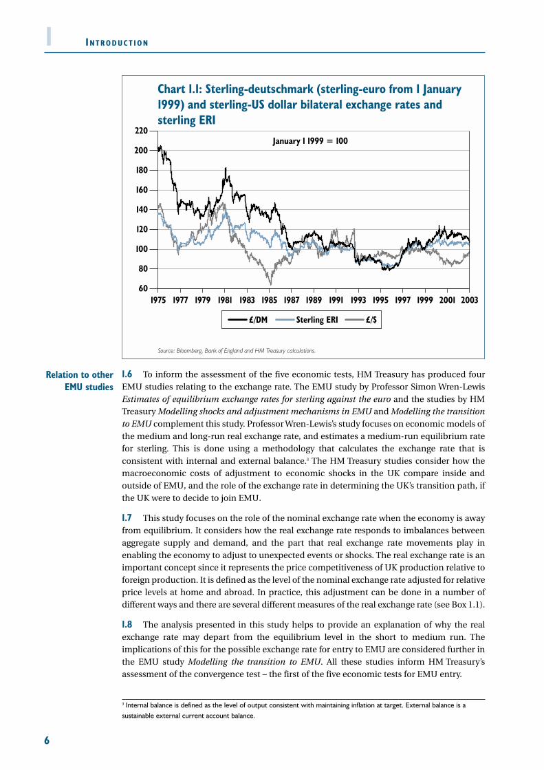
1.5 Chart 1.1 shows the bilateral nominal exchange rates of sterling-deutschmark (sterling-euro from 1 January 1999), sterling-US dollar and the sterling exchange rate index (ERI)2 since1975. It is clear that the exchange rate is fairly volatile. The question is the extent to whichthese movements in nominal, and real, exchange rates are stabilising responses to actual, orperceived, changes in fundamental factors affecting the economy, and the extent to whichthey are simply unwarranted and destabilising shocks. This issue was not considered in detailin the October 1997 assessment of the Government’s five economic tests (HM Treasury, 1997).However, the issue is more prominent now, partly due to the persistent strength of sterling inrelation to the euro during much of the intervening five and a half years.
3 Internal balance is defined as the level of output consistent with maintaining inflation at target. External balance is asustainable external current account balance.
IN T R O D U C T I O N
1.6 To inform the assessment of the five economic tests, HM Treasury has produced fourEMU studies relating to the exchange rate. The EMU study by Professor Simon Wren-LewisEstimates of equilibrium exchange rates for sterling against the euro and the studies by HMTreasury Modelling shocks and adjustment mechanisms in EMU and Modelling the transitionto EMU complement this study. Professor Wren-Lewis’s study focuses on economic models ofthe medium and long-run real exchange rate, and estimates a medium-run equilibrium ratefor sterling. This is done using a methodology that calculates the exchange rate that isconsistent with internal and external balance.3 The HM Treasury studies consider how themacroeconomic costs of adjustment to economic shocks in the UK compare inside andoutside of EMU, and the role of the exchange rate in determining the UK’s transition path, ifthe UK were to decide to join EMU.
1.7 This study focuses on the role of the nominal exchange rate when the economy is awayfrom equilibrium. It considers how the real exchange rate responds to imbalances betweenaggregate supply and demand, and the part that real exchange rate movements play inenabling the economy to adjust to unexpected events or shocks. The real exchange rate is animportant concept since it represents the price competitiveness of UK production relative toforeign production. It is defined as the level of the nominal exchange rate adjusted for relativeprice levels at home and abroad. In practice, this adjustment can be done in a number ofdifferent ways and there are several different measures of the real exchange rate (see Box 1.1).
1.8 The analysis presented in this study helps to provide an explanation of why the realexchange rate may depart from the equilibrium level in the short to medium run. Theimplications of this for the possible exchange rate for entry to EMU are considered further inthe EMU study Modelling the transition to EMU. All these studies inform HM Treasury’sassessment of the convergence test – the first of the five economic tests for EMU entry.
6
1
Relation to otherEMU studies
Chart 1.1: Sterling-deutschmark (sterling-euro from 1 January 1999) and sterling-US dollar bilateral exchange rates and sterling ERI
Source: Bloomberg, Bank of England and HM Treasury calculations.
60
80
100
120
140
160
180
200
220
20011999199719951993199119891987198519831981197919771975 2003
£/$Sterling ERI£/DM
January 1 1999 = 100

7
1.9 The study is structured as follows:
• Section 2 of the study considers how the exchange rate is determined;
• Section 3 considers the role of the exchange rate in the adjustment process,and also the question as to whether nominal exchange rate flexibility providesan additional source of shocks to the economy;
• Section 4 examines the empirical evidence on the role of the exchange rate;
• Section 5 provides an interpretation of sterling’s strength against the eurosince 1996;
• Section 6 looks at how the overall volatility of the exchange rate mightcompare inside and outside of EMU;
• Section 7 sets out the study’s conclusions on the role of the exchange rate;
• Annex A presents the results of a new structural vector autoregression (SVAR)model of the UK economy; and
• Annex B examines the weightings used to construct the UK ERI.
IN T R O D U C T I O N1Box 1.1: Nominal, real and effective exchange rates
A number of different exchange rate concepts are used in this study.
Nominal exchange rates are the rates that are determined in the currency markets.They simply represent the price of one currency in terms of another.
Real exchange rates adjust the nominal exchange rate to take account of cross-countrydifferences in price levels. By using different measures of prices, different real exchangerate measures can be derived. There are two main approaches:
• the first approach is relevant for assessing the extent to which nominal exchangerate movements affect the price competitiveness of its exports. If country A has ahigher inflation rate than country B, then its products will lose pricecompetitiveness unless there is an offsetting depreciation of its nominal exchangerate. Real exchange rate measures based on price measures such as relative exportprices or relative unit labour costs show whether a nominal exchange rate changehas changed a country’s price competitiveness or merely served to offset the effectof difference in inflation rates; or
• alternatively, measures based on relative consumer prices provide an indication ofhow nominal exchange rate changes have affected consumers’ purchasing power.Such measures include the prices of goods and services that are not traded acrossborders.
Effective (or trade-weighted) exchange rate indices are a weighted average ofbilateral exchange rates. For example, if sterling appreciated against the euro butdepreciated against the dollar, the effective exchange rate provides a measure of whetherthese movements cancel each other out or not. The weights in an effective exchange rategenerally reflect the relative importance of different foreign currencies for the homecountry’s trade. Effective exchange rate indices can be constructed either as a weightedaverage of nominal bilateral exchange rates or real bilateral exchange rates.
Structure of thestudy

8

2 MO D E L S O F E XC H A N G E R AT E
D E T E R M I N AT I O N
9
2.1 This section contains a brief review of models of exchange rate determination,emphasising the role of product market and asset market demands in influencing the overallsupply of and demand for different currencies. The section also examines theunpredictability of short-term movements in the exchange rate and considers how this isrelated to the efficient markets principle.
2.2 At any point in time, the exchange rate moves to clear the supply of, and demand for,currencies. For analytical purposes, it is helpful to distinguish between the demand forforeign currency associated with product market flows and the demand associated with assetmarket flows. By focusing on each of these in turn, economic theory has developed plausiblemodels of the factors that determine exchange rates in the short, medium and long term.
2.3 For the purposes of this study, the short term simply reflects the existing state of theeconomy; the medium term reflects expectations as to how the economy will evolve, as theeconomy adjusts to bring aggregate supply and demand into balance, and the long termreflects the further evolution of the economy in response to slower moving trends, such aschanges in demographic structure.1 By combining these theories, it is possible to provide acoherent view of exchange rate determination. However, as is explained below, that does notmake exchange rates predictable, particularly over short horizons.
At any point in time, the exchange rate is determined in the currency markets, as the pricewhich clears the supply of and demand for currencies. The aggregate supply and demandfor currency is generated by different types of transaction: trade in goods and services,investment income flows and asset market transactions.
The uncovered interest parity (UIP) condition states that the interest rate differentialbetween two currencies must be equal to the expected change in the exchange ratebetween those currencies. This suggests that interest rate differentials provide someinformation about expected short-term movements in the exchange rate, and also that thecurrent exchange rate should be determined in large part by expectations of its futurevalue. But it provides no information about what influences these expectations.
Purchasing power parity (PPP) provides a long run explanation of exchange rate levels. Itstates that the exchange rate moves to equate the price of goods across countries.However, there are several reasons, both theoretical and empirical, why PPP may not holdover shorter time horizons.
Macroeconomic models note that the exchange rate must move to balance the externalbalance of payments and that this will entail balancing current account flows with financialaccount flows. This balancing will determine the level of the exchange rate.
To the extent that misalignments in relation to the medium-term level assist the short runadjustment process, they may not be undesirable. But large and persistent deviations frommedium-term levels may be of greater concern, since they may affect the equilibrium towhich the economy eventually returns.
Over the short term, no structural model of the exchange rate provides better forecastsof future exchange rates than simple models which predict the exchange rate will beunchanged from current levels. This has sparked research into characteristics of foreignexchange markets that may explain why the exchange rate moves independently offundamentals over the short run.
1 The EMU study by HM Treasury The five tests framework considers various different definitions of the short, medium andlong run, and their relevance to analysis of EMU.
MO D E L S O F E XC H A N G E R AT E D E T E R M I N AT I O N
2.4 Financial asset holders aim to maximise their return from holding either domestic oroverseas assets. The return from holding overseas assets depends on both the nominal returnfrom these assets, in foreign currency terms, and the expected capital gain from movementsin the exchange rate. In perfect capital markets and abstracting from risk, this leads to theuncovered interest parity condition (UIP), which states that the interest rate differentialbetween two currencies (comparing domestic and foreign assets that have the samecharacteristics apart from their currency of denomination) must be equal to the expectedchange in the exchange rate between those currencies. Hence if interest rates were onepercentage point higher in the UK than in the euro area, the expected return on holdingsterling and euro area assets would only be equal if investors expected sterling to depreciateby one per cent over the following 12 months.
2.5 This relationship suggests that interest rate differentials should determine the path thatthe exchange rate is expected to take in the future. But it also highlights that the expectedfuture value of the exchange rate is an important influence. This determines not only theeventual level of the exchange rate, but also, when combined with the expected paths ofdomestic and foreign interest rates, the current level of the exchange rate. Hence the UIPcondition needs to be combined with theories that consider medium and long-terminfluences on the exchange rate, with the UIP relation helping to explain the path by whichthe exchange rate is expected to adjust to its long term level.
2.6 Purchasing power parity (PPP) provides a long run explanation of exchange rate levels.It states that the exchange rate moves to equate the price of goods across countries. Supposethere was just one, uniformly traded, good and transport costs were zero. If this good couldbe bought more cheaply overseas than in the UK, everyone would buy the good overseas. Thedemand for sterling would fall, leading to a depreciation, which would continue until the twogoods had the same sterling price.
2.7 There are several reasons, both theoretical and empirical, why PPP may not hold. Theextent to which purchasing power parity holds depends on how easy it is to engage inarbitrage when price differentials exist. This varies considerably depending on thecharacteristics of individual goods and services. Many financial instruments can bearbitraged readily and at low cost, while arbitraging of goods and services may be slow andcostly. This may be a result of the time and cost required to set up distribution networks.Arbitrage opportunities may also be affected by transport costs, regulations and currency risk.For a more detailed discussion see the EMU study by HM Treasury Prices and EMU.
2.8 PPP, in terms of consumer prices, would also break down if consumers’ preferencesdiffered between countries (so they bought a different basket of goods). For goods that aretraded, barriers to trade will also lead to a ‘home bias’ in consumption, causing an effectsimilar to that arising from different preferences. In addition, if producers of any type of goodhave market power, then this will enable them to price to market (see Section 3), so the mark-up on costs becomes specific to the destination where the goods are sold. A fuller account ofthe theory of PPP can be found in the EMU study by Professor Simon Wren-Lewis Estimatesof equilibrium exchange rates for sterling against the euro.
2.9 Macroeconomic balance models highlight the fact the exchange rate must move tobalance the external balance of payments. This will entail balancing current account flowswith financial account flows.
10
2
Arbitrage inproduct
markets:purchasing
power parity
Macroeconomicbalance models
Arbitrage inasset markets:
uncoveredinterest parity

11
2.10 The EMU study by Professor Simon Wren-Lewis Estimates of equilibrium exchange ratesfor sterling against the euro uses a medium-term version of this approach. It considers theexchange rate consistent with internal and external balance, where internal balance isdefined as the level of output consistent with maintaining inflation at target, and externalbalance as a sustainable external current account balance. These additional conditions maynot be satisfied in the short run, when the economy is in the process of adjusting to a supplyor demand shock, but they need to be satisfied once the adjustment processes are complete.
2.11 Deviations of the exchange rate from its medium to long run levels are often viewed asmisalignments or evidence of over or under valuation. Such descriptions need to beinterpreted with care. In particular, it is important to recognise that deviations of theexchange rate from its medium or long-term level may be an important part of the processthat restores equilibrium following a shock, just as fluctuations of the real interest rate aroundits long-run level can help to bring the economy back to balance.2 To the extent thatmisalignments in relation to the medium term level assist the short-run adjustment process,they may not be undesirable (see Section 5). But large and persistent deviations frommedium-term levels may be of greater concern, since they may affect the equilibrium towhich the economy eventually returns.
2.12 Although the models discussed above provide valuable insights into exchange ratedetermination, they are only of limited use in making short-term predictions of futureexchange rate movements. In practice, exchange rates have exhibited much greater volatilityover short-term horizons than these models would suggest. Analysis presented in Section 6shows that the sterling-euro exchange rate has typically fluctuated by 1.3 per cent around itsaverage value over a 60 day period, and the US dollar-euro exchange rate by 2 per cent (Table6.1). It should be noted that these are average values, and in some periods the fluctuation hasbeen much greater, and in other periods much less.
2.13 Meese and Rogoff (1983) found that no structural model of the exchange rate, includingvariants of all the models described above, could provide better forecasts of future exchangerates than a simple ‘random walk’ model that predicts that the exchange rate will beunchanged from its existing level. Subsequent research suggests that the explanatory powerof structural models is superior over the long run, which is consistent with the idea that, forexample, PPP holds over the long run. And some researchers are now optimistic about theforecasting ability of short and medium-run models. Nonetheless, the conclusion that, overshort-run time horizons, the current level of the exchange rate is as good a predictor of futureexchange rates as other models is generally accepted.3
2.14 The efficient markets hypothesis provides an explanation of why exchange rate changesare difficult to predict. Markets are considered to be efficient if prices incorporate all publiclyavailable information, including expectations of future policies. If the price of an asset weregenerally expected to rise tomorrow, traders, anticipating this, would buy the asset today. Thiswould drive the price of the asset up until the total expected return was the same. If themarkets were not efficient, the possibility of making arbitrage profits would exist, and traderscould consistently make quick speculative gains. In efficient markets, the possibility ofmaking speculative gains still exists but, provided that the individual trader does not haveprivileged information that is unavailable to the market as a whole, any speculative positionis as likely to yield losses as gains.
MO D E L S O F E XC H A N G E R AT E D E T E R M I N AT I O N2
2 The EMU study Modelling shocks and adjustment mechanisms in EMU examines in detail the role that the exchange rateplays in facilitating this adjustment.3 Taylor (1995), and Frankel and Rose (1995) contain comprehensive reviews of empirical studies of exchange rates.Meese and Rogoff (1983) showed that structural models are poor predictors of future exchange rates. Mark (1995) andChinn and Meese (1996) find evidence that they work better over long horizons. Macdonald (1999) suggests that shortand medium term models can help to improve forecasts. Frankel and Rose (1995) conclude that “the Meese and Rogoffanalysis at short horizons has never been convincingly overturned or explained”.
Exchange ratemisalignments
Exchange ratepredictability ...
... and the role ofthe market
MO D E L S O F E XC H A N G E R AT E D E T E R M I N AT I O N
2.15 If this is the case, then movements in the exchange rate away from the expected pathgiven by UIP should be driven by unanticipated developments (including economic shocks).These should be equally likely to cause the exchange rate to appreciate as to depreciate.Empirical evidence suggests that the effect of such unpredictable information will tend todominate the short-term predictability arising from the UIP condition.4
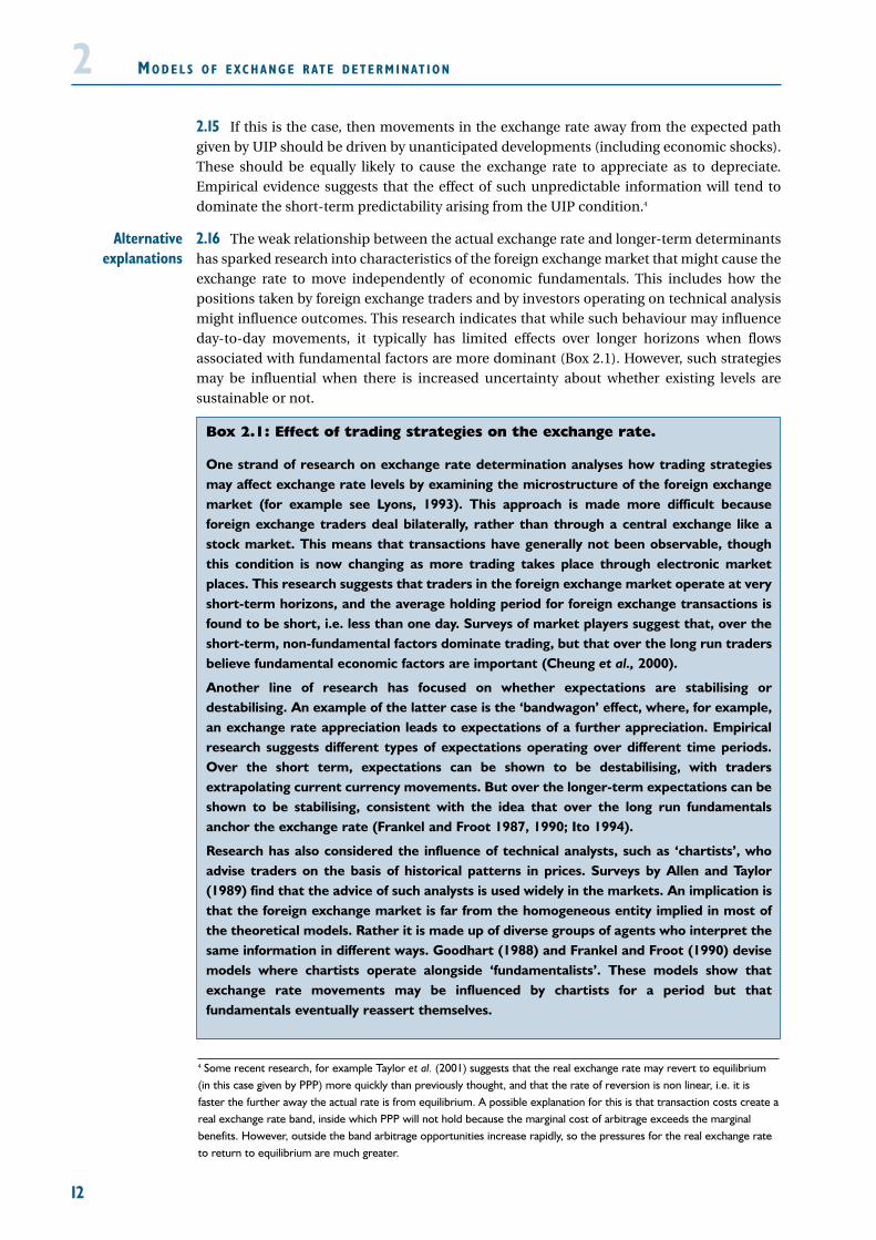
2.16 The weak relationship between the actual exchange rate and longer-term determinantshas sparked research into characteristics of the foreign exchange market that might cause theexchange rate to move independently of economic fundamentals. This includes how thepositions taken by foreign exchange traders and by investors operating on technical analysismight influence outcomes. This research indicates that while such behaviour may influenceday-to-day movements, it typically has limited effects over longer horizons when flowsassociated with fundamental factors are more dominant (Box 2.1). However, such strategiesmay be influential when there is increased uncertainty about whether existing levels aresustainable or not.
12
2
Box 2.1: Effect of trading strategies on the exchange rate.
One strand of research on exchange rate determination analyses how trading strategiesmay affect exchange rate levels by examining the microstructure of the foreign exchangemarket (for example see Lyons, 1993). This approach is made more difficult becauseforeign exchange traders deal bilaterally, rather than through a central exchange like astock market. This means that transactions have generally not been observable, thoughthis condition is now changing as more trading takes place through electronic marketplaces. This research suggests that traders in the foreign exchange market operate at veryshort-term horizons, and the average holding period for foreign exchange transactions isfound to be short, i.e. less than one day. Surveys of market players suggest that, over theshort-term, non-fundamental factors dominate trading, but that over the long run tradersbelieve fundamental economic factors are important (Cheung et al., 2000).
Another line of research has focused on whether expectations are stabilising ordestabilising. An example of the latter case is the ‘bandwagon’ effect, where, for example,an exchange rate appreciation leads to expectations of a further appreciation. Empiricalresearch suggests different types of expectations operating over different time periods.Over the short term, expectations can be shown to be destabilising, with tradersextrapolating current currency movements. But over the longer-term expectations can beshown to be stabilising, consistent with the idea that over the long run fundamentalsanchor the exchange rate (Frankel and Froot 1987, 1990; Ito 1994).
Research has also considered the influence of technical analysts, such as ‘chartists’, whoadvise traders on the basis of historical patterns in prices. Surveys by Allen and Taylor(1989) find that the advice of such analysts is used widely in the markets. An implication isthat the foreign exchange market is far from the homogeneous entity implied in most ofthe theoretical models. Rather it is made up of diverse groups of agents who interpret thesame information in different ways. Goodhart (1988) and Frankel and Froot (1990) devisemodels where chartists operate alongside ‘fundamentalists’. These models show thatexchange rate movements may be influenced by chartists for a period but thatfundamentals eventually reassert themselves.
4 Some recent research, for example Taylor et al. (2001) suggests that the real exchange rate may revert to equilibrium(in this case given by PPP) more quickly than previously thought, and that the rate of reversion is non linear, i.e. it isfaster the further away the actual rate is from equilibrium. A possible explanation for this is that transaction costs create areal exchange rate band, inside which PPP will not hold because the marginal cost of arbitrage exceeds the marginalbenefits. However, outside the band arbitrage opportunities increase rapidly, so the pressures for the real exchange rateto return to equilibrium are much greater.
Alternativeexplanations

3 MACROECONOMIC ADJUSTMENT UNDER
FIXED AND FLOAT ING EXCHANGE RATES
13
3.1 This section reviews how nominal exchange rate changes impact on the widereconomy, with a particular focus on whether or not the exchange rate moves to stabilise theeconomy when there is an imbalance between aggregate supply and aggregate demand:
• the starting point is a review of optimal currency area (OCA) theory whichinvestigates the conditions under which nominal exchange rate flexibilitymay enable an economy to adjust to macroeconomic imbalances moreefficiently than fixed exchange rates;
• the second subsection considers how flexible exchange rates may promotemacroeconomic adjustment, comparing this with how real exchange rateadjustment is achieved when nominal exchange rates are fixed;
• the third subsection considers how the pass-through from exchange ratesinto domestic prices may affect the extent to which exchange rate movementspromote macroeconomic adjustment; and
• the final subsection considers contexts in which exchange rate flexibility failsto promote macroeconomic adjustment, and the argument that exchangerate flexibility more often destabilises than stabilises the economy, notablywhen volatile asset market flows dominate exchange rate movements.
Opt imal currency areas
3.2 Economists have long debated the merits of fixed versus flexible exchange rates. One ofthe central themes of this debate has been whether flexible exchange rates provide amechanism that allows economies to make adjustments to economic change anddisturbances, or whether the exchange rate is itself a source of volatility to the economy. This
Under both floating and fixed nominal exchange rate regimes, the real exchange rateprovides one of the adjustment mechanisms that balances aggregate demand andaggregate supply in the medium and long run.
When nominal exchange rates are fixed, all of the adjustment in real exchange rates isbrought about by differential movements in domestic and foreign price levels.
When nominal exchange rates are flexible, part or all of any real exchange rate adjustmentmay be achieved through adjustment of nominal exchange rates.
Even though the pass-through from exchange rate changes into consumer prices is slow inthe UK, the pass-through into the domestic prices of intermediate goods and import pricesis relatively rapid. This provides a channel through which exchange rate changes affectpurchasing, supply and investment decisions.
The foreign exchange market is dominated by asset market flows. Some have argued thatthis makes flexible exchange rates an additional source of shocks to the economy.
But asset market flows are likely to reflect the strength or weakness of economic activityin different countries. Asset inflows into strong economies will tend to contribute to anexchange rate appreciation, and outflows from weak economies to contribute to anexchange rate depreciation. Hence it is likely that exchange rate movements generated byasset market flows will, on average, tend to assist macroeconomic adjustment.

MAC R O E C O N O M I C AD J U S T M E N T UN D E R F I X E D A N D FLOAT I N G EXC H A N G E RAT E S
debate led to the theory of optimal currency areas, first set out by Mundell in 1961, whichaddresses the issue of how best to choose which geographical areas should share a singlecurrency.1
3.3 OCA theory suggests that the balance of advantages and disadvantages between fixedand floating exchange rates varies according to the manner and extent of economicintegration between countries. It identifies those features that tend to favour countriesmaintaining fixed exchange rates and those that tend to favour flexible exchange rates.Flexible exchange rates would be preferred where they enhance the ability of the economy toabsorb economic shocks. Fixed exchange rates would be preferred where their benefitsoutweigh the additional cost of achieving macroeconomic adjustment via other mechanisms,such as relative wage and price movement and/or factor mobility.
3.4 OCA theory assumes that factors of production, such as labour and capital, are mobileinternally but immobile externally. For example, it is assumed that labour moves betweenregions of an OCA, but does not move significantly into or out of the OCA. OCA theory alsoassumes that there is limited price and wage flexbility in the economy. With limited price andwage flexibility, it is the the internal mobility of factors of production which allows the OCA’seconomy to adjust smoothly to an internal asymmetric shock. For example, if demand for agood produced in a sub-region of the OCA falls, mobility of labour prevents unemploymentfrom occurring in the sub-region.
3.5 Because it is assumed that factors are not as mobile externally, this adjustmentmechanism cannot stabilise the economy following a shock with asymmetric effects on thedomestic and foreign economies. Instead, and in the absence of price and wage flexibility,stabilisation is achieved by adjustment of the nominal exchange rate, which brings about thenecessary adjustment of the real exchange rate to restore balance of payments equilibrium.An OCA hit by a shock that decreases demand for its exports would undergo a nominalexchange rate depreciation, as decreased foreign demand for exports drives down the price ofdomestic currency. This depreciation will decrease the price of exports and so increaseforeign demand, countering the impact of the shock without causing domesticunemployment. Conversely, a positive demand shock will lead to a nominal exchange rateappreciation rather than cause domestic inflation.
3.6 In each case, nominal exchange rate flexibility has smoothed the effects of a shock;preventing inflation in the case of the positive demand shock, and unemployment in the caseof the negative demand shock. The flexible exchange rate has in effect allowed real wages toadjust quickly to a disturbance; this adjustment could not easily take place directly throughwages and prices, due to their limited flexibility.
3.7 The subsequent development of OCA theory has deepened the analysis of theconditions that determine whether the exchange rate is an efficient stabilising mechanism.Various authors have argued that other conditions may affect the OCA criteria, including theextent of trade integration, fiscal integration and whether an economy’s production structureis concentrated in a few industries or is diversified across industries. Mundell (1973) notedthat a common currency could enable different regions to share risks more efficiently.
3.8 Although these extensions provide for a richer analysis, they do not alter the two maininsights from optimal currency area theory, namely:
14
3
Optimal currencyarea theory . . .
. . . and the roleof the exchange
rate
Conclusions onOCA theory
1 The EMU study by HM Treasury The five tests framework has a detailed discussion of the theory of optimal currencyareas. McKinnon (1963) and Kenen (1969) made important early contributions to this literature. McKinnon (2002) andthe contributions of Robert Mundell, Peter Kenen and George Tavlas to the EMU study Submissions on EMU from leadingacademics consider how OCA theory applies to EMU.
15
• the ease with which labour and capital can flow between different activities inresponse to changing patterns of supply and demand will determine how wellan economy can respond to economic shocks; and
• that, under certain conditions, for example in the absence of wage and priceflexibility, exchange rate flexibility may be a useful way of aidingmacroeconomic adjustment.
The exchange rate as a stabi l i s ing mechanism
3.9 This section considers the role of real exchange rate adjustment in stabilising theeconomy under both fixed and floating exchange rate regimes.
3.10 Box 1.1 in Section 1 explains that the real exchange rate is defined as the level of thenominal exchange rate adjusted for relative price levels at home and abroad. When nominalexchange rates are fixed, all of the adjustment in real exchange rates must be brought aboutby differential movements in the domestic and foreign price levels. But when nominalexchange rates are flexible, part or all of any real exchange adjustment may be achievedthrough adjustment of nominal exchange rates.
3.11 The real exchange rate is an important concept, since it represents a country’s terms oftrade – the relative price of domestic and foreign production. Movements in the real exchangerate can therefore influence the balance of supply and demand between domestic and foreigngoods and services. In doing so, real exchange rate adjustment can help to eliminatemacroeconomic imbalances and stabilise the economy.
3.12 At a macroeconomic level, unexpected economic events, or ‘shocks’, affect the balancebetween aggregate demand and aggregate supply. By definition, they will mean that aneconomy that was previously in internal and external balance will no longer be so. Thissection describes the impact of macroeconomic imbalances on the real exchange rate, andhow, in principle, movements in the real exchange rate can act to eliminate the initialimbalances, and hence to stabilise the economy.
3.13 When exchange rates are fixed, and there is a situation where there is excess demand fordomestic production, then upward pressures on the domestic price level will cause the realexchange rate to appreciate. This will encourage a switching of demand towards foreignsuppliers, and a switching of supply towards domestic markets. Both effects reduce, andeventually eliminate, the initial excess demand. A similar argument can be used todemonstrate that a real exchange rate depreciation, brought about by falling relative pricelevels, will eliminate excess supply. If wages and prices are slow to adjust, this could lead toprolonged periods of real exchange rate misalignment. This may be particularly so if therequisite shift in relative prices should require a cut in nominal wage levels domestically, anoutcome that is more likely in a low inflation environment.2
3.14 In other words, when nominal exchange rates are fixed, any adjustment in the realexchange rate that may be needed to maintain or restore macroeconomic balance can onlycome about through differential movements in inflation. That means that if the UK were inEMU, then UK inflation would tend to be higher or lower than the euro area average if a realexchange rate appreciation or depreciation were needed. Such changes have alreadyoccurred within the existing euro area, where inflation in the Netherlands and Ireland hasbeen relatively strong and inflation in Germany relatively weak (see Box 3.1).
MAC R O E C O N O M I C AD J U S T M E N T UN D E R F I X E D A N D FLOAT I N G EXC H A N G E RAT E S3
Effect ofeconomic
shocks
Adjustment in afixed exchange
rate regime
Definition of thereal exchange
rate
2 The possibility that it may be more difficult to achieve a real depreciation than a real appreciation within EMU isconsidered further in the EMU study by Professor Simon Wren-Lewis Estimates of equilibrium exchange rates for sterlingagainst the euro. The issue of wage flexibility is reviewed in the EMU study EMU and labour market flexibility.

MAC R O E C O N O M I C AD J U S T M E N T UN D E R F I X E D A N D FLOAT I N G EXC H A N G E RAT E S
3.15 However, other adjustment mechanisms are also available. The EMU study Modellingshocks and adjustment mechanisms in EMU examines alternative mechanisms that canreduce the required response of the real exchange rate to external shocks when the nominalrate is fixed. The study also further examines how the UK economy would respond to shocksin EMU compared to outside.
3.16 Similar adjustment processes operate in a floating exchange rate regime. But in thiscase, movements in the nominal exchange rate provide an alternative route for achieving therequired real exchange rate adjustment. Some, or indeed all, of the required real exchangerate adjustment may be achieved by an appropriate change in the nominal exchange rate, sothat the required adjustment in domestic and foreign price levels will tend to be smaller.
3.17 A particular case to note is where both the home and foreign economies are followingidentical inflation targets. Under these conditions both monetary authorities will tend toadjust their respective policies to ensure that they meet their targets, with the result that thereal exchange rate adjustment will be predominantly achieved through the nominal exchangerate. By contrast, in a monetary union, when a country experiences a shock that requires itsreal exchange rate with respect to other countries in the union to change, this can only beachieved by a period in which its inflation rate is temporarily above or below inflation in therest of the monetary union.
16
3
Adjustment in afloating
exchange rateregime
Box 3.1: Inflation divergence within the euro area
The experiences of the Netherlands, Ireland and Germany illustrate the point that nationalinflation rates may be different within EMU, depending on whether demand is relativelyweak or relatively strong.
Between 1999 and 2002 euro area inflation averaged 2 per cent a year. But inflation inIreland averaged 4.1 per cent a year and in the Netherlands 3.3 per cent a year. In bothcases these figures were boosted by tax changes, but even allowing for this, their inflationrates remained higher than in other euro area countries. This reflected strong demandgrowth and tight labour markets. By contrast, relatively weak demand growth and highunemployment has contributed to lower inflation in Germany, averaging 1.4 per cent ayear.
Average inflation rates since 1999
1999 2000 2001 2002
Germany 0.6 1.5 2.1 1.3
The Netherlands 2.0 2.3 5.1 3.9
Ireland 2.5 5.3 4.0 4.7
Euro area 1.1 2.1 2.4 2.2
These developments have been recognised as providing each economy with appropriatereal exchange rate changes. For example, Blanchard (2001) argues that inflation had aclear role to play in alleviating excess demand in Ireland and warns against ‘demonising’inflation differentials in EMU. The OECD (2002) concluded that inflation had played animportant role in eroding the overly competitive position of the Netherlands in relation toother euro area countries. Similarly, the European Commission (2001) note that “domesticinflation may well be a desirable part of an adjustment process in a monetary union. If externaldemand is the main source of overheating, inflation is the natural instrument to return toequilibrium”.

17
3.18 The preceding analysis implies a country’s real exchange rate will ultimately reflectunderlying economic conditions, irrespective of whether nominal exchange rates are fixed orfloating. But the adjustment mechanism is different, with adjustment in the domestic pricelevel being greater under a fixed exchange rate regime. Under flexible exchange rates, themovement in the nominal exchange rate can cushion some of the impact on the domesticprice level, and consequently may act as a shock absorber.
Exchange rate changes and domest ic pr ices
3.19 For a flexible nominal exchange rate to act as an effective stabilisation mechanism,nominal exchange rate changes must ‘pass-through’ into changes in the domestic price level.Pass-through is defined as a relationship between the nominal exchange rate and thedomestic price level. If a flexible nominal exchange rate is to operate as an adjustmentmechanism, a nominal depreciation must raise the consumer price of imported goodsrelative to domestic goods, thereby encouraging consumers to buy domestic rather thanforeign goods. But some evidence suggests that nominal exchange rate movements are notfully passed through to consumer prices. This limits the impact on relative prices experiencedby consumers, which determines whether they opt to buy domestic or foreign goods.
3.20 The effect of an exchange rate change on relative prices experienced by domesticconsumers will depend on the pricing strategy of exporting firms:
• the effect is greatest when exporters set prices in domestic currency and thentranslate this price into foreign currency at the prevailing exchange rate(known as producer currency pricing – PCP); or
• an alternative is that an exporting firm keeps its price fixed in foreign currencyand accepts the resulting domestic price at the prevailing exchange rate (thisis local currency pricing – LCP). In this case, a nominal exchange rateappreciation reduces the exporter’s profit margin, but may not affect theconsumer price or the quantity sold in the importing country.
3.21 Exporting firms may use LCP in order to maintain price stability for their consumers.This may occur when firms trading overseas operate in markets dominated by domesticallyproduced goods, and so ‘price to market’. Krugman (1989) argues that if there are high sunkcosts to trading, for example in setting up trading infrastructure and establishingrelationships, then exchange rate fluctuations, within a certain range, are unlikely to cause afirm to exit the market. Rather, firms may remain in the market in the expectation that theexchange rate movement will be temporary. He observes that the large nominal appreciationand then depreciation of the US dollar in the mid 1980s did not have as big an impact on USmanufacturing exports and production as might have been expected. He attributes this inlarge part to the presence of ‘price to market’ strategies.
3.22 A firm’s pricing strategy may also depend on the price elasticity for its goods and on thestructure of costs:
• if demand is price inelastic, the firm may prefer to pass-through a domesticcurrency rate appreciation to the foreign currency price, as the quantity soldwill not fall significantly;
• if demand is price elastic, the firm may prefer to keep the foreign price fixedto maintain output levels; and
MAC R O E C O N O M I C AD J U S T M E N T UN D E R F I X E D A N D FLOAT I N G EXC H A N G E RAT E S3
Pricing strategies
Imperfect pass-through may
reduce theimpact of
nominalexchange rates
Conclusions onreal exchange
rate adjustment
Pricing tomarket

MAC R O E C O N O M I C AD J U S T M E N T UN D E R F I X E D A N D FLOAT I N G EXC H A N G E RAT E S
• similarly, if the firm has increasing returns to scale or high fixed costs, it mayprefer to keep foreign price levels stable in the face of an appreciation in orderto maintain output levels, but there may be some resultant cost to profitmargins that will make it cease to export at all.
3.23 Another explanation for the weak pass-through of exchange rate changes to consumerprices is that for many goods, the production cost of the good is only a small part of the finalprice paid by the consumer. Other costs such as retail, transport, marketing costs may be littleaffected by exchange rate changes.
3.24 For goods and services where local currency pricing is strong, adjustment to exchangerate changes may be primarily driven by the way that firms react to changes in their profitmargins. For example, exporters may decide that margins are too low to continue trading, orlow margins may deter other firms from entering the export market.
3.25 In addition, if imports are intermediate goods then the effect of exchange rate changeson firms’ input costs may be much greater than the effect on consumer prices. If this is thecase, expenditure switching behaviour by firms rather than consumers allows exchange ratesto have an adjustment role.3 For example, importing companies may switch betweendomestic and foreign suppliers in the face of exchange rate changes. Equally, firms that haveproduction facilities in a number of overseas locations may switch the source of imports inthe face of exchange rate changes. In each case, consumer prices may not change after anexchange rate change, but there will have been a change in the demand for foreign anddomestic goods.
3.26 Empirical studies offer evidence in support of the argument that there is not a strongpass-through from exchange rate changes to consumer prices, but that there is at least partialpass-through to import prices:
• McCarthy (2000) looks at surveys of pass-through from exchange rate todomestic inflation, reporting several studies that have found this effect to becomparatively weak. The author then analyses pass-through to domesticinflation for several industrialised countries and finds evidence of only amodest pass-through of the exchange rate to consumer prices — including inthe UK, Germany and France — over the 1980s and 1990s. Debelle andWilkinson (2002) find that pass-through to inflation is also muted, and that inthe case of Australia it has become more muted over the past two decades.However, for the UK the relationship has been fairly constant; and
• Goldberg and Knetter (1996) review the empirical evidence on pass-throughfrom nominal exchange rate changes to import prices. They conclude:“although there is substantial variation across industries, in many cases half ormore of the effect of an exchange rate change is offset by destination specificadjustments of mark-ups over costs” (Goldberg and Knetter 1996, page 37).
3.27 Tables 3.1 and 3.2 reproduce analysis by Kara and Nelson, which presents correlationsbetween nominal UK exchange rates and UK import and consumer prices. Table 3.1 shows aweak relationship between the nominal exchange rate and UK retail price inflation, both overthe period since 1958 and in a sub-sample since 1980. The results hold even after controllingfor the impact of large tax changes on the retail price index. However, there is found to be astronger relationship between UK import prices and the nominal exchange rate (Table 3.2).
18
3
Empiricalevidence on
pass-through
Exchange rateadjustment with
LCP
3 See, for example, Obstfeld (2002).

19
Table 3.1: Correlations between UK retail price inflation and the nominaleffective exchange rate
1958 Q4 – 2002 Q2 0.103
1958 Q4 – 2002 Q2, controlling for 1979 and 1990 tax changes 0.153*
1958 Q4 – 1979 Q2 0.289*
1980 Q1 – 2002 Q2 –0.073
1980 Q1 – 2002 Q2, controlling for 1990 tax changes –0.071*Statistically different from zero at 0.05 significance level.Source: Kara and Nelson, 2002.
Table 3.2: Correlations between UK import price inflation and thenominal effective exchange rate
1958 Q4 – 2002 Q1 0.499*
1958 Q4 – 1979 Q2 0.478*
1980 Q1 – 2002 Q1 0.575**Statistically different from zero at 0.05 significance level.Source: Kara and Nelson, 2002.
3.28 Campa and Goldberg (2002) examine the degree of pass-through from exchange ratesinto import prices across 25 OECD countries. Their main findings are:
• there is strong evidence of partial pass-through in the short run — averagepass-through across countries is around 60 per cent after three months andaround 75 per cent over the longer run;
• UK pass-through is found to be lower than the average at 39 per cent in theshort run and 47 per cent in the long run; and
• there is a trend toward lower pass-through over time, which can mainly beattributed to changes in the composition of imports toward manufacturedgoods as intra-industry trade has increased.
3.29 Taylor (2000) argues that there may be lower pass-through in low inflation countries, asoverseas producers are unlikely to raise prices if they expect relative price stability indomestic prices. If firms are less willing to increase prices where inflation is low and stable,then if EMU is a low inflation environment this may lead to convergence in the degree ofpass-through in participating countries. Campa and Goldberg (2002) find some evidence tosupport Taylor’s hypothesis, though the relationship is found to be weak.
3.30 The substantial empirical evidence on the limited pass through of nominal exchangerate movements has recently led to the development of theoretical models of ‘exchange ratedisconnect’. In these models the presence of LCP alongside some additional assumptionsmeans that the nominal exchange rate becomes entirely ‘disconnected’ from the realeconomy4; movements in the nominal exchange rate do not affect the underlying situation ofthe real economy. This is because low rates of pass-through mean that there is little responseof consumer and producer behaviour to nominal exchange rate movements. In this scenario,a flexible nominal exchange rate is unable to provide the equilibrating real exchange rateadjustment anticipated in the earlier analysis.
MAC R O E C O N O M I C AD J U S T M E N T UN D E R F I X E D A N D FLOAT I N G EXC H A N G E RAT E S3
Exchange rate‘disconnect’
4 See, for example, Devereux and Engel (2002).

MAC R O E C O N O M I C AD J U S T M E N T UN D E R F I X E D A N D FLOAT I N G EXC H A N G E RAT E S
3.31 Overall, pricing to market effects show that the stabilising role of the nominal exchangerate is unlikely to be as straightforward as predicted in simple models. But the evidencesuggests that nominal exchange rates can influence the price of domestic production relativeto foreign production. Studies show that pass-through to domestic inflation is not complete,but that there is significant pass-through to import prices. Firm level adjustment to importprice changes may then provide the necessary economic adjustments. Even assuming fullLCP, firms may adjust trade in the face of movements in profit margins.
3.32 The effect of the existence of pricing to market is to modify rather than eliminate the roleof flexible exchange rates in the adjustment mechanism. It suggests that the stabilising role offlexible rates may operate more gradually and through different channels than simple theorypredicts. But this does not necessarily imply that the additional adjustment mechanismavailable under flexible rates can be relinquished costlessly to a system of fixed exchangerates.
Circumstances where nominal exchange rates do notstabi l i se the economy
3.33 Optimal currency area theory highlights the circumstances in which flexible nominalexchange rates can play an important role in aiding adjustment. However, these particularcircumstances may often not apply. For example, Buiter (1999a) sets out circumstances underwhich flexible exchange rates may not, in practice, serve as a useful adjustment mechanism as:
• nominal exchange rate flexibility does not provide adjustment to imbalancescaused by long-term real rigidities in the economy;
• over the short and medium run the nominal exchange rate often fails to playa stabilisation role; and
• instead, in the short and medium term the exchange rate is frequently anexogenous source of shocks to the economy.
3.34 The first strand of Buiter’s critique is that nominal exchange rate flexibility does notprovide a solution to problems caused by real rigidities. Such rigidities impede the requiredadjustment of relative prices within a currency area, whereas exchange rate changes can onlychange relative prices between currency areas. Real structural problems, such as excessivenon-wage labour costs, rigid industrial structure and weak corporate governance cannot beaddressed through the exchange rate, but only by microeconomic reform. Worse, repeateduse of nominal devaluations may actually delay much needed structural reforms, as theyprovide countries with a short-term way of alleviating the cost of adjustment, which mayappear more attractive than undertaking difficult structural reforms.
3.35 This rightly suggests that exchange rate flexibility does not provide a solution toproblems that require a change in relative prices within the currency area. But this does notmean that nominal exchange rate flexibility does not provide a solution to other problems. Inparticular, as OCA theory highlights, exchange rate flexibility can be helpful in a context whenreal exchange rates need to adjust but the adjustment of domestic and/or foreign prices issluggish. As noted earlier in this section, nominal exchange rate flexibility is the only way inwhich the real exchange rate can change when two authorities are independently targetingtheir domestic price levels.
3.36 The second part of Buiter’s critique is that, in practice, nominal exchange rates havelargely failed to aid the adjustment process in the short and medium term. As already noted,nominal exchange rate flexibility is only helpful when it facilitates the real exchange ratechanges needed to adjust to a particular shock. So it is useful to analyse the contexts underwhich this condition may fail.
20
3
Long-term realrigidities and the
nominalexchange rate
Nominalexchange rateflexibility and
adjustment
Nominalexchange rateflexibility doesnot always aid
adjustment
Conclusion onexchange rates
and domesticprices

21
3.37 The relationship between nominal and real exchange rates is influenced by theopenness of the economy. In an open economy, changes in the nominal exchange rate mayfeed through quickly into the domestic wage and price level. For example, a nominalexchange rate depreciation will raise the price of imported goods. If these account for a highproportion of consumer purchases, and/or of inputs into non-traded goods and services,then the domestic wage and price level may rise in response. This will counteract the impactof the nominal exchange reate depreciation. This gives small, open economies less scope touse nominal exchange rate flexibility as a means of obtaining a real exchange ratedevaluation.5
3.38 The UK is a relatively open economy, with exports and imports each accounting foraround 28 per cent of GDP. But the size of the non-traded sector is sufficiently large to meanthat nominal exchange rate changes are not necessarily offset by changes in UK inflation andespecially so when aggregate demand for UK products is weak.
3.39 The relation between nominal and real exchange rate changes varies according tocontext, including the pressures that are causing the exchange rate to move. If the domesticeconomy is already operating at full capacity, domestic prices will tend to rise in response tothe extra demand created by a nominal depreciation, taking the real exchange rate back to itsinitial level. But if the domestic economy is operating at below full capacity, domestic priceswill tend to rise by less than the initial nominal depreciation, leading to a sustained realdevaluation. Indeed during the past fifteen years the UK has experienced large and persistentchanges in its real exchange rate (Box 3.2).
The exchange rate as a source o f shocks
3.40 The third part of Buiter’s critique is that the exchange rate is determined primarily bydevelopments in the international capital market. While these flows may take the exchangerate in the same direction as required to achieve product market equilibrium, they do notnecessarily do so. In his view, capital market developments subject the nominal exchange rateto large and persistent changes that may have little relation to imbalances in productmarkets. This reduces the effectiveness of a flexible exchange rate as a stabilising mechanism.
MAC R O E C O N O M I C AD J U S T M E N T UN D E R F I X E D A N D FLOAT I N G EXC H A N G E RAT E S3
5 This issue is addressed in Mundell (1961), which acknowledges that the size of an economy puts a lower limit on thesize of an OCA. Mundell notes that a smaller economy is likely to have a higher proportion of imports in totalconsumption, and so more likely to see wages rise in response to a nominal exchange rate depreciation.
Asset marketflows as a
potential sourceof shocks
Box 3.2: Nominal and real exchange rate changes in the UK
In the past fifteen years, there have been two striking episodes where the context in whicha large movement in the nominal exchange rate has occurred has enabled a persistentchange in the real exchange rate:
• the sharp decline in the nominal exchange rate in 1992 was not eroded by anincrease in domestic inflation, since it occurred in the context of substantial excesssupply in the UK market; and
• the sharp appreciation of the exchange rate in 1997 did not lead to an equivalentdrop in the UK price level, since it occurred against the backdrop of strongdemand for UK production.
In the first instance, recovery from the 1990-92 recession would probably have been muchmore subdued, and may have been delayed, if sterling had not depreciated. And in thesecond instance, inflationary pressures would probably have been much stronger hadsterling not appreciated. The historical evidence on the link between the exchange ratesand macroeconomic conditions in the UK is considered further in Section 4. Section 5contains a more detailed appraisal of sterling’s appreciation in 1997.

MAC R O E C O N O M I C AD J U S T M E N T UN D E R F I X E D A N D FLOAT I N G EXC H A N G E RAT E S
Indeed, in some circumstances capital market developments may lead to an exchange ratechange that exacerbates rather than reduces imbalances in product markets.
3.41 In a currency union, the way in which asset market demands are transmitted is different.Those asset market flows that are motivated by the desire to either hedge currency risk, or toexploit the chance that the nominal exchange rate may change, no longer exist. However,even in the absence of floating exchange rates there is still the possibility that country specificrisk premia6 may emerge in asset prices. But since cross-border demands for both financialand real assets will no longer be transmitted through the currency markets, they will impactdirectly on individual asset market prices. As they will no longer affect exchange rates withinthe monetary union, the spillover to price signals in product markets will no longer exist.
3.42 The argument that asset market flows may lead to exchange rate changes that areinconsistent with product market equilibrium is potentially a valid one. But it does notnecessarily follow that asset market flows are, in practice, destabilising. Asset market flows aredetermined by investors’ wish to create and maintain portfolios that adequately balance riskand return. While investors are far from omniscient, they are not, as a group, wilfullyirrational.7
3.43 Investor rationality implies that asset markets should not misprice the exchange rateconsistently, nor indeed any other asset price. Cross-currency asset flows are determined byinvestors’ evaluations of the relative value of assets in each currency area. These in turn arelikely to reflect the underlying strengths and weaknesses of economic activity within eachcurrency area.
3.44 In short, asset prices, including exchange rates, are unlikely to be strong when theeconomy is weak, and vice-versa. This argument provides theoretical grounds for questioningwhether the exchange rate is as frequently or as powerfully a source of shocks as is sometimesclaimed. Section 4 considers the empirical evidence on the issue.
Conclus ions
3.45 Under both fixed and floating exchange rate regimes, a real exchange rate change maybe required to enable the economy to adjust to a disturbance to the balance of aggregatesupply and demand. This will generally be the case when the disturbance is asymmetricacross countries. Optimal currency area theory analyses the conditions in which nominalexchange rate adjustment may be a more efficient way of achieving real exchange rateadjustment than by allowing inflation rates to differ for a period.
3.46 The chief advantage of a flexible exchange rate regime is that price adjustment in theforeign exchange market reacts rapidly to changes in the supply and demand for a country’sgoods, services and assets. This may be especially desirable when the alternative, under afixed exchange rate system, would entail lower inflation than in other countries, andpotentially wage cuts. However, under both regimes the real effects on the economy will bethe same; real relative prices are adjusting even if it is nominal exchange rates that arefacilitating the adjustment.
22
3
6 A risk premium is the difference between the expected rate of return on an investment and the risk-free return (e.g. ona government stock) over the same period. If there were any risk element at all (e.g. in investing in a particular country),both the price of the asset and the rate of return would be higher than that if no risk is involved.7 In other words, their investment decisions will typically have a rational base, even if subsequent developments lead tosome expectations being disappointed. Actual outcomes only consistently match expected outcomes when there iscertainty. In an uncertain world, actual outcomes will more often than not either exceed or disappoint expectations.When this happens, it does not necessarily mean that the initial expectations were ill-founded, since expectations need toprice in all possible outcomes, including those that fail to materialise.
Transmission ofasset market
related shocksunder currency
unions
23
3.47 In theory, flexible exchange rates may not always act to stabilise the economy, and somehave argued that they tend more often to be destabilising. However, asset market demandsare, in general, likely to reflect the underlying strengths and weaknesses of economic activitywithin each currency area. Consequently they will tend to push the exchange rate up whenthe economy is strong and cause a depreciation when the economy is weak. Such movementsshould boost the stabilising properties of flexible exchange rates. The next section considersthe empirical evidence relating to this question.
MAC R O E C O N O M I C AD J U S T M E N T UN D E R F I X E D A N D FLOAT I N G EXC H A N G E RAT E S3

24

4 EMPIRICAL EVIDENCE ON THE
STABIL IS ING ROLE OF EXCHANGE RATES
25
4.1 This section considers various methods that have been used to analyse the extent towhich movements in nominal exchange rates have helped to stabilise or destabilise theeconomy, with particular reference to the UK.
4.2 The problem that empirical studies of this issue face is how to distinguish betweenwarranted and unwarranted movements of the exchange rate. This turns out to be lessstraightforward to do than it might appear. This section first presents and reviews somedescriptive analyses of exchange rate movements over the past thirty years. It then goes on toreview econometric studies that use more technically sophisticated econometric techniquesto consider this question.
4.3 Sterling’s nominal exchange rate has fluctuated considerably over the past thirty years.Between 1975 and 1995 it depreciated by 29 per cent against the US dollar and 59 per centagainst the deutschmark, and between 1995 and 2002 it depreciated by a further 5 per centagainst the US dollar but appreciated by 38 per cent against the deutschmark (Chart 4.1).These movements, and those of sterling against the UK’s other trading partners are reflectedin the sterling exchange rate index (ERI). When sterling moves in a different direction againstthe dollar than against the euro, the exchange rate index will be less volatile than the bilateralexchange rate, as has been the case, for example, since 1999.1 During the 1970s, nominal andreal exchange rate movements were weakly correlated, as inflation outcomes in the UKdiffered substantially from those in other major economies. More recently, the narrowing ofinflation differentials has meant that the correlation between the nominal and real exchangerate has strengthened (Chart 4.2).
The relation between exchange rate movements and the business cycle appears fairlyweak. But with the exception of the early 1980s, nominal exchange rate movements do notappear to have destabilised the economy.
Academic research has found that macroeconomic volatility is largely unrelated towhether a country has a fixed or floating exchange rate.
Econometric analysis of the unexpected movements in UK output, prices and exchangerates does not support the proposition that a flexible exchange rate provides an additionalsource of shocks to the economy.
Without observing the counter-factual of what would have happened if the exchange ratehad not moved, it is difficult to say how big a shock absorbing role it plays.
But it is likely that adopting a permanently fixed exchange rate (as in EMU) would meanthat pressures that are currently absorbed by the exchange rate would have to beabsorbed by other adjustment mechanisms.
1 The ERI is an example of an effective exchange rate index (see Box 1.1). Annex B illustrates how different weightingschemes affect the volatility of such measures.
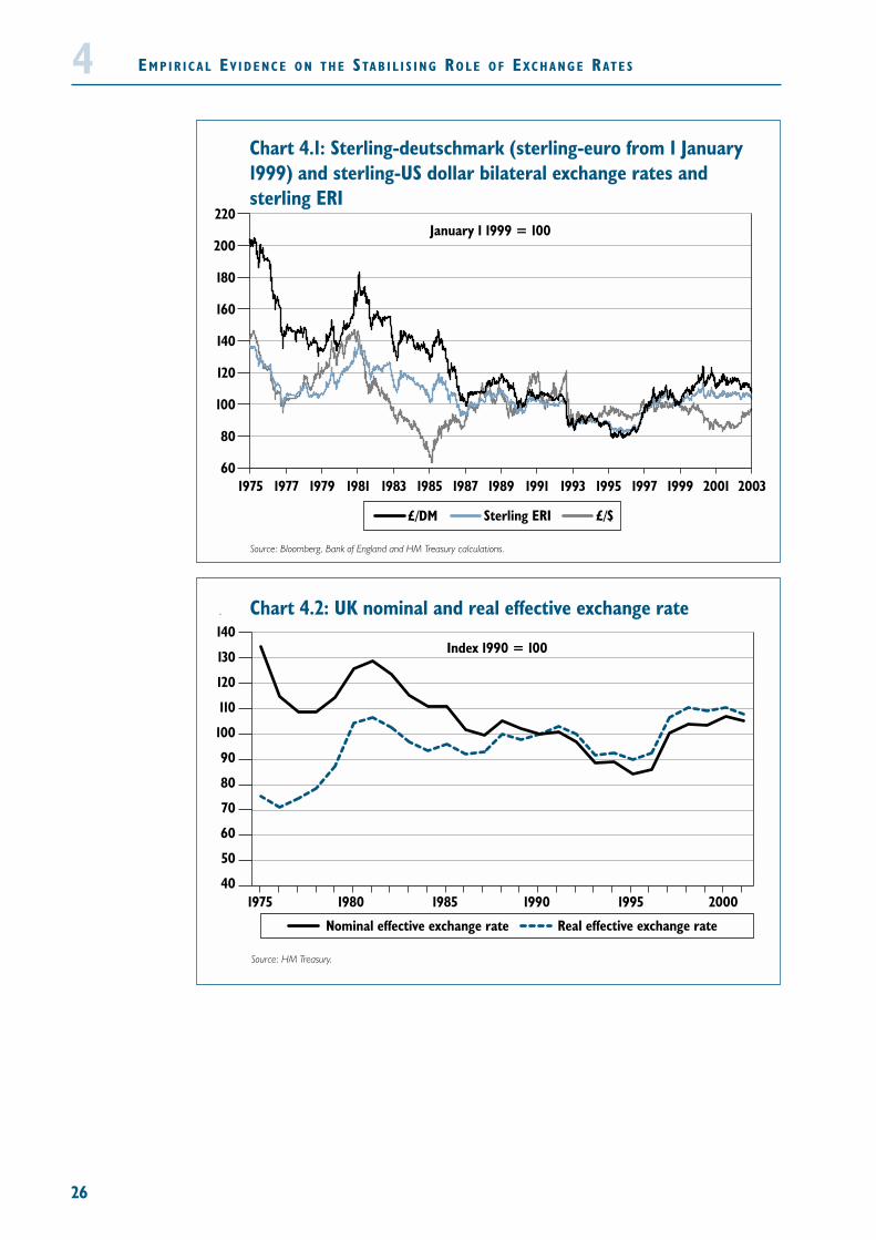
EM P I R I C A L EV I D E N C E O N T H E STA B I L I S I N G RO L E O F EXC H A N G E RAT E S
26
4
Chart 4.2: UK nominal and real effective exchange rate
Source: HM Treasury.
40
50
60
70
80
90
100
110
120
130
140
Real effective exchange rateNominal effective exchange rate
200019951990198519801975
Index 1990 = 100
Chart 4.1: Sterling-deutschmark (sterling-euro from 1 January 1999) and sterling-US dollar bilateral exchange rates andsterling ERI
Source: Bloomberg, Bank of England and HM Treasury calculations.
60
80
100
120
140
160
180
200
220
20011999199719951993199119891987198519831981197919771975 2003
January 1 1999 = 100
£/$Sterling ERI£/DM

27
Exchange rate movements and the bus iness cyc le
4.4 In order to stabilise economic activity, sterling’s real exchange rate should, other thingsequal, appreciate when demand is stronger in the UK than in its main trading partners, anddepreciate when it is weaker.
4.5 In practice, the correlation between sterling’s exchange rate and its relative demand(measured by its relative output gap2), has been weak (Charts 4.3 and 4.4). That said, with twonotable exceptions, sterling’s movements do not seem to have been particularly destabilising.Indeed, over extended periods it has moved in a direction consistent with the UK’s relativecyclical position:
• between 1981 and 1986 the UK’s relative cyclical position was weak andsterling depreciated in both nominal and real terms;
• between 1986 and 1990 the real exchange rate appreciated when the UKrelative cyclical position was strong. The nominal exchange rate was broadlystable over this period, with most of the real appreciation attributable tohigher inflation in the UK than in our main trading partners;
• between 1992 and 1993 the real exchange rate depreciated when the UKrelative cyclical position was weak. The nominal exchange rate depreciationafter sterling left the ERM was an important component of the realdepreciation; and
• between 1994 and 1996 and also between 1998 and 2002 the UK cyclicalposition was broadly the same as in other major countries and sterling’sexchange rate remained approximately stable in both real and nominal terms.
EM P I R I C A L EV I D E N C E O N T H E STA B I L I S I N G RO L E O F EXC H A N G E RAT E S4
Chart 4.3: UK real exchange rate and relative output gap
-6
-4
-2
0
2
4
6
60
70
80
90
100
110
120
1975 20001995199019851980
Source: OECD, JP Morgan, HM Treasury calculations.
Outp
ut g
ap, p
er c
ent o
f GDP
Real
exc
hang
e ra
te, 1
990=
100
Real exchange rateRelative output gap
Exchange ratemovements and
the businesscycle
2 The relative output gap for the UK is its output gap (the difference between its actual and potential output) minus theweighted average output gap of the US, Germany and Japan, using GDP weights.

EM P I R I C A L EV I D E N C E O N T H E STA B I L I S I N G RO L E O F EXC H A N G E RAT E S
4.6 The two episodes where the real exchange rate change appears to have beendestabilising were:
• between 1978 and 1981, when the exchange rate appreciated sharply eventhough the UK cyclical position was relatively weak. During this period, therewere strong upward pressures from the rapid improvement in the UK’sbalance of payments on oil, and from the tight monetary policy stance; and
• between 1990 and 1992, when the real exchange rate remained approximatelyconstant despite the UK’s relatively weak cyclical position. During this period,sterling’s nominal exchange rate was constrained by participation in the ERM.
4.7 The other striking feature of this analysis is that sterling’s strong appreciation between1996 and 1998 appears unrelated to the cyclical position. With the relative output gap close tozero between 1995 and 1998, an appreciation of this scale does not appear to have beenneeded to stabilise the cyclical position. But nor did the appreciation cause the cyclicalposition to deteriorate.
4.8 On balance, this evidence does not offer much support to the view that nominalexchange rate movements tend to be a significant source of shocks to the economy. But theextent to which nominal exchange rate movements help to stabilise the economy appears tovary over time. Nominal depreciations in the early 1980s and after 1992, and the nominalappreciation between 1996 and 1998, were key components of the respective real exchangerate adjustments, while at other times real exchange rates have tended to be driven bydifferences between UK and foreign inflation.
4.9 In a similar analysis of exchange rate changes and the business cycle in the mainindustrial economies, the IMF (1998) reached similar conclusions:
“there does appear to be a positive correlation between currency movements and thebusiness cycle in several prominent episodes. ... At other times, however, the correlationbetween exchange rates and the cycle is less apparent or even negative” (page 62).
28
4
-6
-4
-2
0
2
4
6Chart 4.4: UK nominal exchange rate and relative output gap
1975 20001995199019851980
Source: OECD, JP Morgan, HM Treasury calculations.
Outp
ut g
ap, p
er c
ent o
f GDP
Nom
inal
exc
hang
e ra
te, 1
990=
100
Nominal exchange rateRelative output gap
60
70
80
90
100
110
120
130
140

29
4.10 Cobham (2002) argues that exchange rate changes have not generally helped to stabilisethe economy. He analyses whether movements in sterling were expected or welcomed by theUK monetary authorities, and concludes:
“... the exchange rate has not generally functioned as a useful automatic equilibratingmechanism or as a useful policy instrument; ... in nearly every phase there weremovements of the exchange rate, or pressures on it, which for the authorities wereunexpected and unwelcome. Thus the exchange rate has typically been a source ofextraneous shocks” (page 70).
4.11 Cobham’s analysis is based on deviations of the real exchange rate from its long-runaverage, and does not include explicit consideration of the cyclical position of the economy.For the real exchange rate to act as a stabilising mechanism, it should be expected to departfrom its equilibrium level when there is either excess supply or excess demand in theeconomy. Departures of the exchange rate from its long run average do not necessarily equateto destabilising movements, just as departures of the interest rate from a neutral policy stanceare not necessarily destabilising. Without relating exchange rate movements to theunderlying cyclical position, it is not possible to reach a meaningful conclusion as to whetherparticular movements are acting as an equilibrating mechanism.
4.12 Neither does the observation that exchange rate movements were unexpected andunwelcome to the authorities help to resolve the question as to whether the exchange rate isa source of extraneous shocks. While consistent with the proposition that the exchange rate isa source of shocks, it is also consistent with the alternative proposition that exchange ratemovements are one of the channels through which shocks to the economy are transmitted.Either way, the fact that exchange rate movements are unexpected is consistent with theefficient markets hypothesis, which implies that exchange rate movements should beunpredictable (see Section 2). The finding that the authorities do not tend to welcomeexchange rate movements is consistent with their existing policy stance having already beenaligned with their previous reading of economic conditions.
4.13 Hence while Cobham’s analysis provides interesting insights into the history of UKmonetary policy, the evidence it provides does not prove that the exchange rate has typicallybeen a source of extraneous shocks.
EM P I R I C A L EV I D E N C E O N T H E STA B I L I S I N G RO L E O F EXC H A N G E RAT E S4Exchange rate
changes andmonetary policy

EM P I R I C A L EV I D E N C E O N T H E STA B I L I S I N G RO L E O F EXC H A N G E RAT E S
Macroeconomic vo lat i l i ty under d i f ferent exchange ratearrangements
4.14 Flood and Rose (1999) note that a number of researchers have attempted to assesswhether countries with flexible exchange rates are more vulnerable to economic shocks thancountries with fixed exchange rates. They summarise these studies as follows:
“there is remarkably little evidence of a systematic relationship between the exchange rateand measurable macroeconomic phenomena…Simply put…countries with fixedexchange rates have less volatile exchange rates than floating countries, but macro-economies that are equally volatile” (page 661).
4.15 This evidence could be interpreted as showing that having a flexible exchange rate doesnot expose countries to additional sources of shocks. But it could also be interpreted asshowing that flexible exchange rates are no better at absorbing shocks than fixed regimes.
4.16 These interpretations are not mutually exclusive, particularly if the existingconfiguration of exchange rate regimes broadly satisfies the optimal currency area criteria. Ifthis is the case, then countries with fixed exchange rate regimes should be able to absorbshocks without the need for nominal exchange rate adjustment, while countries with flexiblerates should find it easier to allow some adjustment through the nominal exchange rate.
Econometr ic ident i f i cat ion o f the source o f shocks
4.17 Another way to analyse exchange rate volatility is to use econometric techniques toidentify how different shocks impact on the economy. Various studies have used thetechnique of structural vector autoregressions (SVAR) to do this. The SVAR technique usesstatistical methods to analyse the relationship between a set of variables and the shocks thatimpinge on them. In the analyses considered below the set of variables generally includesmeasures of the exchange rate, output and inflation, and in some cases, the interest rate.
4.18 A number of studies have used this technique to investigate the extent to whichexchange rate movements tend to be associated with movements in other economic variableseither immediately or in the longer-term:
• a finding that large exchange rate changes tend to have big effects on outputand prices, and that it tends to move in an inappropriate direction, (i.e. toappreciate when the currency was weak or depreciate when it was strong),would indicate that exchange rate movements tend to be destabilising;
• a finding that large exchange rate movements tend to have big effects onoutput and prices, and tend to move in an appropriate direction would beconsistent with exchange rate movements having a strong stabilising role; and
• a finding that large exchange rate movements tend not to be associated withmovements in other economic variables would be consistent with it acting asa shock absorber. This is because a shock absorber should take the impact offorces that would otherwise have other effects.
4.19 A number of approaches have been used to analyse the relation between the exchangerate and other variables. These are described in more detail below and in Annex A, whichdescribes a model constructed by HM Treasury. This model investigates the interaction of UKoutput, prices, the short-term interest rate and the real exchange rate. It uses two differentapproaches to identify shocks that loosely follow the approaches of Clarida and Gali (1994)and Artis and Ehrmann (2000), which are explained in Box 4.1 and Box 4.2.
30
4
Macroeconomicvolatility under
differentexchange ratearrangements
Econometricanalyses: the
SAVR technique

31
EM P I R I C A L EV I D E N C E O N T H E STA B I L I S I N G RO L E O F EXC H A N G E RAT E S44.20 Despite the differences in approach, the various studies find that large exchange ratechanges are not typically associated with changes in output or the price level. This finding ismost consistent with the shock absorber explanation. It suggests that exchange rate changestend to deflect some of the impact that demand shocks might otherwise have had.
4.21 The SVAR technique can be used to analyse the extent to which the economy respondsto particular shocks. This is done by considering the contribution of each shock to the errorsmade in forecasting each variable. Studies of the UK exchange rate have tended to attribute ahigh proportion of unexpected exchange rate movements to asymmetric demand shocks(Tables 4.1 and 4.2). The exception to this is Artis and Ehrmann, who define demand shocksdifferently from the other studies (see Box 4.2). The HM Treasury SVAR model can replicateboth findings, by defining demand shocks in a similar fashion to Clarida and Gali (HMTreasury 1) or in a similar fashion to Artis and Ehrmann (HM Treasury 2).3 The Treasury SVARmodel is described in Box 4.3 and in more detail in Annex A.
Box 4.1: Clarida and Gali’s SVAR model
Clarida and Gali (1994) used the SVAR methodology to investigate the relationship betweenreal exchange rates, relative output and relative price levels for a number of countries,including the UK. They identified three structural shocks as follows:
• relative supply shocks comprising all shocks that had a permanent effect on the levelof output in the UK relative to output in the US;
• relative demand shocks comprising all remaining shocks that had a permanenteffect on the level of the real exchange rate; and
• relative nominal shocks comprising all remaining shocks.
These definitions mean that all three structural shocks can have permanent effects onrelative price levels, whereas only supply and demand shocks can permanently affect thereal exchange rate, and only supply shocks can permanently affect relative output levels.These restrictions only apply to permanent effects. This means that all three structuralshocks may have a temporary effect on output, prices or the real exchange rate. These‘temporary’ effects may be quite long-lasting. They are temporary in the sense that they arenot permanent, rather than in the sense that they only persist for a short period.
Exchange ratevolatility
3 Annex A shows that the properties of the exchange rate shock in the HM Treasury 2 breakdown and the demand shockin the HM Treasury 1 breakdown are similar, despite the difference in their labels. See Labhard and Westaway (2002) fora more detailed investigation of this finding.

EM P I R I C A L EV I D E N C E O N T H E STA B I L I S I N G RO L E O F EXC H A N G E RAT E S
32
4Box 4.2: Artis and Ehrmann’s SVAR model
Artis and Ehrmann (2000) use the SVAR approach to identify the source of shocks and theirimpact on four economies – Denmark, Sweden, Canada and the UK. Each of theseeconomies has large neighbours with whom a monetary union has been mooted at somepoint. Their analysis measures the effect on output in these economies of monetary policy,inflation, the exchange rate and other exogenous shocks.
Artis and Ehrmann apply the SVAR methodology differently from the Clarida-Galiapproach:
• they analyse more variables (output, price level, domestic interest and foreigninterest rates and the nominal exchange rate);
• they model the nominal exchange rate rather than real exchange rate;
• they model UK output and price levels independently of output and prices in othercountries, whereas Clarida and Gali modelled the difference between UK and USoutput and the difference between UK and US prices. As a result, Artis andEhrmann’s model captures all shocks to UK output and prices, whereas Clarida andGali only capture shocks that have a different effect on output and prices in the UKcompared with other contries; and
• they define demand shocks as being all shocks, other than supply shocks, that havean immediate impact on GDP. This differs from the Clarida and Gali definition,which identifies demand shocks as all shocks, other than supply shocks, that have apermanent effect on the real exchange rate.
These differences imply:
• that some of their ‘nominal shocks’ have permanent effects on real exchange rates– and hence would be defined as ‘demand shocks’ if Clarida and Gali’s definitionswere used; and
• that their nominal shocks also include effects of German supply and demand shocks(since these do not affect UK output in the long run nor UK output immediately,but should impact on the exchange rate).a
Artis and Ehrmann’s results are strikingly different from those in the Clarida-Gali tradition.In particular, they find that exchange rate unpredictability is predominantly due to nominalshocks rather than demand shocks (Tables 4.1 and 4.2).
Artis and Ehrmann’s decomposition identifies three nominal shocks: a domestic monetarypolicy shock, a foreign monetary policy shock, and an exchange rate shock. The exchangerate shock accounts for all exchange rate movements that are not associated with a UKsupply shock, UK demand shock or policy shocks in the UK or Germany. Artis and Ehrmannfind that pure exchange rate shocks account for around three-fifths of exchange ratevolatility, at both short and longer term forecast horizons.a See Labhard and Westaway (2002) for a detailed exposition of this point.
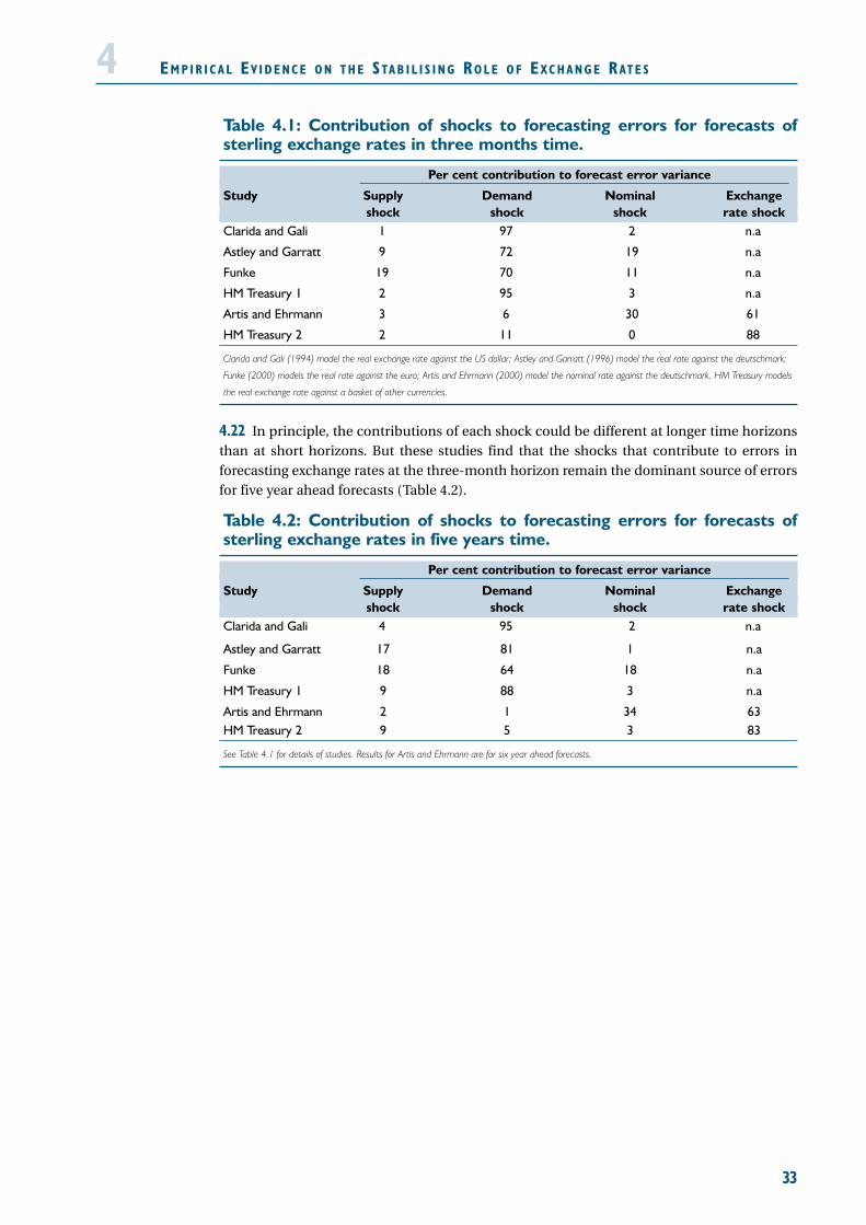
33
Table 4.1: Contribution of shocks to forecasting errors for forecasts ofsterling exchange rates in three months time.
Per cent contribution to forecast error variance
Study Supply Demand Nominal Exchange shock shock shock rate shock
Clarida and Gali 1 97 2 n.a
Astley and Garratt 9 72 19 n.a
Funke 19 70 11 n.a
HM Treasury 1 2 95 3 n.a
Artis and Ehrmann 3 6 30 61
HM Treasury 2 2 11 0 88
Clarida and Gali (1994) model the real exchange rate against the US dollar; Astley and Garratt (1996) model the real rate against the deutschmark;
Funke (2000) models the real rate against the euro; Artis and Ehrmann (2000) model the nominal rate against the deutschmark. HM Treasury models
the real exchange rate against a basket of other currencies.
4.22 In principle, the contributions of each shock could be different at longer time horizonsthan at short horizons. But these studies find that the shocks that contribute to errors inforecasting exchange rates at the three-month horizon remain the dominant source of errorsfor five year ahead forecasts (Table 4.2).
Table 4.2: Contribution of shocks to forecasting errors for forecasts ofsterling exchange rates in five years time.
Per cent contribution to forecast error variance
Study Supply Demand Nominal Exchange shock shock shock rate shock
Clarida and Gali 4 95 2 n.a
Astley and Garratt 17 81 1 n.a
Funke 18 64 18 n.a
HM Treasury 1 9 88 3 n.a
Artis and Ehrmann 2 1 34 63HM Treasury 2 9 5 3 83
See Table 4.1 for details of studies. Results for Artis and Ehrmann are for six year ahead forecasts.
EM P I R I C A L EV I D E N C E O N T H E STA B I L I S I N G RO L E O F EXC H A N G E RAT E S4

4.23 Most studies find that supply shocks are the main contributor to the unpredictability ofoutput in three month ahead forecasts (Table 4.3). The HM Treasury SVAR is an exception inthis respect. This may be because Clarida and Gali, Astley and Garratt and Funke all model thedifference in output between the UK and other countries, whereas the HM Treasury SVARmodels the level of UK output. However, Artis and Ehrmann also model the level of UKoutput, but still find that a relatively high proportion of output variability can be accountedfor by supply shocks.
34
EM P I R I C A L EV I D E N C E O N T H E STA B I L I S I N G RO L E O F EXC H A N G E RAT E S4Box 4.3: HM Treasury SVAR model
HM Treasury has constructed an SVAR model to illustrate how alternative approaches toderiving the underlying shocks to the economy provide different perspectives on theireffects on the exchange rate and other macroeconomic variables. Like Artis and Ehrmann(2000), the model analyses UK GDP and prices, and hence illustrates the effects of all shocksimpacting on the UK, whereas Clarida and Gali’s model only captures asymmetric shocks(that is shocks that have a greater or lesser effect on UK output and prices than they do inother countries).
Two alternative approaches have been used to derive the underlying shocks to the economy.Both approaches identify supply shocks as all shocks that have a permanent effect on thelevel of UK output, but they differ in the way that they derive the remaining shocks.
The first approach (HM Treasury 1) derives a shock that accounts for all remaining shocksthat have a permanent effect on the level of the real exchange rate, as in Clarida and Gali(1994). This accounts for a high proportion of exchange rate unpredictability, both in theshort term and over longer term horizons (Tables 4.1 and 4.2). This result closely resemblesthat of the original Clarida and Gali study.
The second approach (HM Treasury 2) derives a demand shock that accounts for all shocks,other than the supply shock, that have an immediate effect on the level of output, and anexchange rate shock that accounts for remaining unexplained movements in the realexchange rate. These definitions broadly follow those used by Artis and Ehrmann (2000).Under this scheme, the exchange rate shocks account for most of the unpredictability ofexchange rates (Tables 4.1 and 4.2). This result closely resembles that of Artis and Ehrmann.
Comparison of the two schemes shows that they identify shocks with broadly similarproperties, although by different routes. In particular, both schemes identify a single shockthat accounts for almost all of the variation in the exchange rate. And in both schemes thisshock has moderate effects on output, prices and interest rates. In other words, bothapproaches imply that exchange rate changes have not been a significant source of shocksto the wider economy.
Annex A contains more details about the model and how it illustrates the effects of differentshocks on the economy.
Output volatility
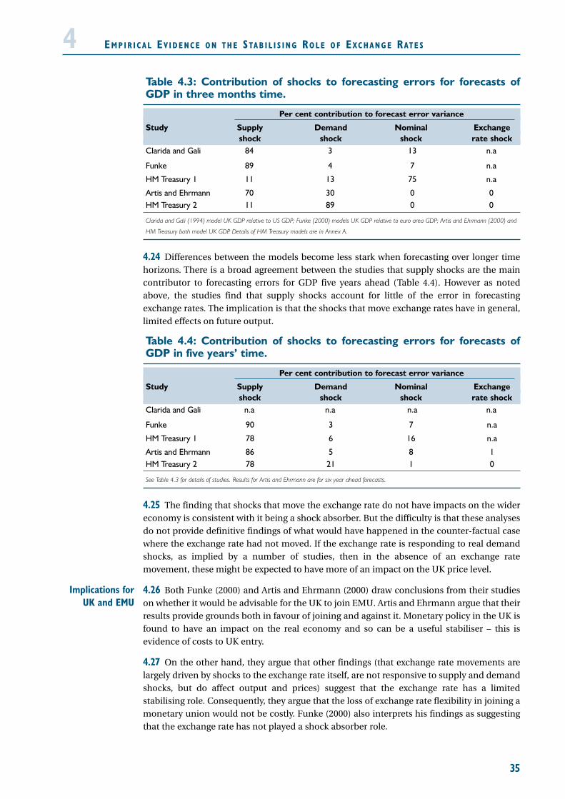
35
Table 4.3: Contribution of shocks to forecasting errors for forecasts ofGDP in three months time.
Per cent contribution to forecast error variance
Study Supply Demand Nominal Exchange shock shock shock rate shock
Clarida and Gali 84 3 13 n.a
Funke 89 4 7 n.a
HM Treasury 1 11 13 75 n.a
Artis and Ehrmann 70 30 0 0HM Treasury 2 11 89 0 0
Clarida and Gali (1994) model UK GDP relative to US GDP; Funke (2000) models UK GDP relative to euro area GDP; Artis and Ehrmann (2000) and
HM Treasury both model UK GDP. Details of HM Treasury models are in Annex A.
4.24 Differences between the models become less stark when forecasting over longer timehorizons. There is a broad agreement between the studies that supply shocks are the maincontributor to forecasting errors for GDP five years ahead (Table 4.4). However as notedabove, the studies find that supply shocks account for little of the error in forecastingexchange rates. The implication is that the shocks that move exchange rates have in general,limited effects on future output.
Table 4.4: Contribution of shocks to forecasting errors for forecasts ofGDP in five years’ time.
Per cent contribution to forecast error variance
Study Supply Demand Nominal Exchange shock shock shock rate shock
Clarida and Gali n.a n.a n.a n.a
Funke 90 3 7 n.a
HM Treasury 1 78 6 16 n.a
Artis and Ehrmann 86 5 8 1HM Treasury 2 78 21 1 0
See Table 4.3 for details of studies. Results for Artis and Ehrmann are for six year ahead forecasts.
4.25 The finding that shocks that move the exchange rate do not have impacts on the widereconomy is consistent with it being a shock absorber. But the difficulty is that these analysesdo not provide definitive findings of what would have happened in the counter-factual casewhere the exchange rate had not moved. If the exchange rate is responding to real demandshocks, as implied by a number of studies, then in the absence of an exchange ratemovement, these might be expected to have more of an impact on the UK price level.
4.26 Both Funke (2000) and Artis and Ehrmann (2000) draw conclusions from their studieson whether it would be advisable for the UK to join EMU. Artis and Ehrmann argue that theirresults provide grounds both in favour of joining and against it. Monetary policy in the UK isfound to have an impact on the real economy and so can be a useful stabiliser – this isevidence of costs to UK entry.
4.27 On the other hand, they argue that other findings (that exchange rate movements arelargely driven by shocks to the exchange rate itself, are not responsive to supply and demandshocks, but do affect output and prices) suggest that the exchange rate has a limitedstabilising role. Consequently, they argue that the loss of exchange rate flexibility in joining amonetary union would not be costly. Funke (2000) also interprets his findings as suggestingthat the exchange rate has not played a shock absorber role.
EM P I R I C A L EV I D E N C E O N T H E STA B I L I S I N G RO L E O F EXC H A N G E RAT E S4
Implications forUK and EMU

4.28 But the conclusion that these studies demonstrate that the exchange rate is not asignificant shock absorber is puzzling. Artis and Ehrmann argue that “if variable X perfectlystabilises shocks which could impinge on variable Y then the ex post data will reveal variationsin X but none in Y but it would be a mistake to conclude that X was ineffective as a shockabsorber!”(page 6). Yet having made this point, they appear to ignore it when they evaluate therole of the exchange rate.
4.29 This strand of analysis cannot conclusively resolve the question as to whether theexchange rate is or is not a shock absorber, since we can only observe what happens when theexchange rate actually moves. But the presumption that all other variables would beunaffected (and hence that the exchange rate is not responding to an otherwise unobservedshock) is a strong one. Without evidence that demonstrates that other variables would havebeen unaffected if the exchange rate had not moved, the conclusion that the exchange ratefails to act as a shock absorber is, at best, unproven.
Conclus ions
4.30 The evidence considered in this section suggests that nominal exchange rate flexibilitydoes not typically generate additional macroeconomic volatility. Econometric studies usingthe SVAR technique suggest that exchange rate movements do not, in general, destabilise theeconomy. This supports the conclusion drawn from more qualitative analysis of the relationbetween exchange rates and the relative cyclical position. On balance, there is little evidenceto support the proposition that exchange rate flexibility provides an additional source ofshocks.
4.31 Whether exchange rate flexibility is a significant stabilising mechanism or not is harderto resolve. The econometric evidence finds that large exchange rate movements do nottypically affect other macroeconomic variables. This could be because they are helping toabsorb an otherwise unobserved shock. But it could be that observed exchange ratemovements are purely extraneous. Without observing what would have happened had theexchange rate not moved, it is not possible to resolve the question conclusively. But it seemsunlikely that real exchange movements would not have real effects, and therefore likely thatobserved exchange rate changes have helped to absorb shocks that might otherwise haveimpacted on either output or prices.
4.32 The finding that countries with fixed exchange rate regimes do not experience highermacroeconomic volatility than countries with flexible exchange rates confirms the insightfrom OCA theory that fixed regimes are viable, provided that alternative mechanisms (forexample, wage and price flexibility, flexible redeployment of resources to alternative uses andfiscal stabilisation) enable a rapid adjustment to economic shocks.
36
EM P I R I C A L EV I D E N C E O N T H E STA B I L I S I N G RO L E O F EXC H A N G E RAT E S4

5 AN IN T E R P R E TAT I O N O F T H E
ST R E N GT H O F ST E R L I N G S I N C E 1996
37
5.1 In recent years, sterling’s exchange rate against the euro exceeded most estimates of itssustainable exchange rate for an extended period. Nonetheless, the economy continued toperform well on most indicators (Chart 5.1). GDP growth averaged 2.6 per cent a yearbetween 1996 and 2002, inflation remained close to its target and unemployment fell from 7.5per cent in January 1997 to 5.1 per cent in November 2002. This performance is consistentwith the conclusion from Section 4 that large exchange rate movements have not typicallybeen a source of shocks to the economy.
In recent years, sterling remained persistently above most estimates of its sustainable rateagainst the euro. Nonetheless, at a whole economy level, the effects on UK output andprices appeared limited. This section considers whether these outcomes provide groundsfor thinking that the sustainable exchange rate has appreciated in recent years, or forthinking that a temporary appreciation relative to the longer-term sustainable rate mayhave been warranted.
The macroeconomic balance framework defines the sustainable exchange rate as the ratethat should prevail when the economy satisfies two conditions, representing internalbalance (aggregate demand matches aggregate potential supply) and external balance(the external current account flows can be sustainably financed). Neither condition needhold at a particular point in time, although when either condition fails, prices andquantities will tend to adjust to eliminate the imbalances over time. While theseadjustment processes are operating, deviations of the actual exchange rate from itssustainable rate may be warranted. Both the magnitude and the duration of deviations ofthe actual rate from its sustainable level will depend on the extent and persistence of thefactors causing the internal and external balance conditions to fail.
During the past few years, demand for UK goods and services has been relatively strongcompared with demand for euro area goods and services, in part reflecting the relativestrength of UK domestic demand. This differential in relative demand has warranted adegree of sterling real exchange rate appreciation against the euro, both to prevent theUK economy overheating and to bolster demand for euro area production.
With both the UK and the euro area monetary authorities pursuing broadly similar pricestability objectives, real exchange rate movements between the two currency areas weremainly achieved by movements in the nominal exchange rate. By contrast, if the UK hadbeen in EMU, any real exchange rate change between the UK and the current euro areacountries would have needed to occur through differential price movements. It is likelythat UK inflation would have been higher than it was.
Up until the end of 2002, some argued that sterling’s equilibrium real exchange rate hadappreciated relative to the range of previous estimates. However, sterling’s depreciationduring early 2003 is more supportive of the view that its strength in recent years may havebeen a temporary, albeit protracted, move away from longer-term equilibrium. It isimportant to emphasise that interpretation of recent movements is made more difficult byuncertainties about both the scale and persistence of market reactions to the particularlyhigh degree of global political and economic uncertainty.
Nonetheless, this appreciation may have been warranted by a persistent decrease in netnational saving, associated with relatively strong domestic demand growth in the UKcompared with the euro area. These explanations are considered further in theconvergence test – the first of the Government’s five economic tests for EMU entry.
1996-2002:strong sterling
and a strongeconomy

AN IN T E R P R E TAT I O N O F T H E ST R E N GT H O F ST E R L I N G S I N C E 1996
5.2 That said, the strong exchange rate clearly affected the performance of certain sectors.The volume of exports of goods and services grew by 4.3 per cent a year between 1996 and2002 compared with import growth of 7.1 per cent a year, and manufacturing output grewmore slowly than services output and actually declined in 2001 and 2002. Nonetheless, overallmacroeconomic performance held up well, despite the difficulties experienced by individualsectors. One interpretation of this is that a real exchange rate appreciation may have beenneeded in order to maintain macroeconomic balance, by attracting labour and otherresources into the industries where they were most needed.
5.3 Understanding recent trends is an important part of assessing what might be theappropriate rate at which sterling should be fixed against the euro, were a decision taken tojoin EMU. The EMU study by Professor Simon Wren-Lewis Estimates of equilibrium exchangerates for sterling against the euro highlights that fixing at too high an exchange rate couldmean that the early years of EMU membership would be characterised by low output growthin order to obtain the low inflation needed to secure a real depreciation within EMU. Bycontrast, entering at too low an exchange rate could mean that the early years of EMUmembership would see relatively high UK inflation and a real exchange rate appreciation.These scenarios, together with possible policy responses, are illustrated in detail in the EMUstudy Modelling the transition to EMU. The EMU study Modelling shocks and adjustmentmechanisms in EMU illustrates real exchange rate adjustment within EMU itself.
38
5
Chart 5.1: UK GDP growth, inflation and the sterling-euro exchange rate
Source: Office for National Statistics, Bloomberg.
0
1
2
3
4
5
2001200019991998199719961995 20021.0
1.4
1.6
1.8
GDP growth Inflation (RPIX) €/£ exchange rate (RHS)
Per cent €/£

39
5.4 The analysis in this section uses recent exchange rate history to illustrate why actualexchange rates may deviate from their estimated sustainable rates for extended periods oftime. The analysis focuses on sterling’s exchange rate against the euro. This is in large partbecause sterling has moved more sharply against the euro than against the US dollar in recentyears. Indeed, sterling has tended to depreciate against the US dollar when it has appreciatedagainst the euro, and to appreciate against the US dollar when it has depreciated against theeuro, so that movements in the trade-weighted exchange rate have been more muted thansterling’s movements against the euro. Although the focus of this section is on the sterling-euro exchange rate, the principles discussed can be used to analyse exchange ratemovements more generally.
5.5 Bilateral exchange rates are a relative price: the sterling-euro exchange rate is the priceof sterling in terms of euro. As such, movements in the exchange rate reflect economicconditions in both currency areas.
5.6 The Government believes that exchange rate stability can only be achieved on the basisof sound economic fundamentals, in particular low and steady inflation, steady andsustainable growth and sound public finances. The exchange rate is, therefore, an outcomethat reflects other economic policies, both in the UK and in other countries.
Pr ice stabi l i ty and changes in the rea l exchange rate
5.7 An important point to note is that both the UK and the European monetary authoritieswere pursuing price stability in their respective currency areas during the period consideredin this analysis. As a result, there was limited scope for inflation differences to bring about anyreal exchange rate change between the UK and Europe that may have been needed. Thismeant that nominal exchange rate movements were the main channel for securing realexchange rate changes.
5.8 In other words, the foreign exchange rate market plays an important role in achievingreal exchange adjustment when monetary authorities are committed to achieving pricestability in their respective currency areas. This is especially the case when the requiredchange in the real exchange rate is large. For example, in the absence of any nominalexchange rate change, a 10 per cent real appreciation in the sterling-euro real exchange ratewould require either a 10 per cent increase in the UK price level or a 10 per cent fall in the euroarea price level, or an appropriate combination of price level movements in the two areas. Inany of these scenarios, monetary authorities would find it difficult to convince the public thatthey still had a strong and credible commitment to maintaining price stability.
Deviat ions o f the exchange rate f rom susta inablemedium-term leve ls
5.9 The sharp depreciation of sterling that followed its exit from the ERM in September 1992appeared consistent with the view that the ERM parity of 2.95 DM/£ was unsustainably high(Wren-Lewis et al., 1991). Sterling remained below 2.50 DM/£ for most of the following fouryears.
AN IN T E R P R E TAT I O N O F T H E ST R E N GT H O F ST E R L I N G S I N C E 19965
Sterling’s ERMparity:
unsustainablyhigh…

AN IN T E R P R E TAT I O N O F T H E ST R E N GT H O F ST E R L I N G S I N C E 1996
5.10 But towards the end of 1996 sterling began to appreciate again. By July 1997, theexchange rate had risen back above the 2.95 DM/£ level, reaching a peak of over 3.30 DM/£ inMay 2000, and averaging 1.62 €/£ (equivalent to 3.16 DM/£) between 2000 and 2002. Thislevel was well above estimates of the sustainable exchange rate, many of which rangedbetween 1.2 and 1.4 A/£, equivalent to 2.35 and 2.74 DM/£, respectively.1 Estimates based onpast data have tended to provide lower figures for the equilibrium rate than other estimates,such as surveys of City economists, some of which have suggested that the sustainable ratecould be as high as 1.55 A/£ (3.03 DM/£). But even these estimates imply that sterling wastrading above its equilibrium rate between 1998 and 2002. Its subsequent depreciation duringearly 2003 has brought it within the range indicated by the survey evidence, althoughremaining, in mid March, above the 1.4 A/£ level.
5.11 This prompts the question as to why sterling deviated from estimates of its sustainablerate for so long. Explanations can be divided into two categories:
• estimates of the sustainable medium-term exchange rate remained valid, butthere were strong and persistent pressures that took the actual exchange rateaway from its sustainable level for an extended period; and
• alternatively, the sustainable exchange rate may have been higher thanpreviously estimated. For example, an analysis by the IMF concluded that “thepersistence of the real exchange rate appreciation observed in the UnitedKingdom over the past few years ... suggests that the equilibrium real exchangerate may have appreciated” (IMF, 2002, page 68).
5.12 Estimates of the sustainable exchange rate provide an indication of the exchange ratethat is expected to prevail when economic adjustment to shocks has run its course and anyassociated imbalances have been eliminated. For example, the estimates derived by ProfessorSimon Wren-Lewis in his EMU study Estimates of equilibrium exchange rates for sterlingagainst the euro are derived on the basis that there is no imbalance between aggregatedemand and aggregate supply, and that net national saving (that is national saving lessnational investment) is at a sustainable level. Neither condition need apply at any particularmoment, and the actual exchange rate may deviate from its estimated equilibrium rate untilboth conditions are satisfied.
5.13 In the macroeconomic balance framework, deviations of the actual exchange rate fromits longer-term rate are warranted when either the internal balance or external balanceconditions are not satisfied. Under current arrangements, UK and European interest rates areaimed at maintaining or restoring internal balance within their respective currency areas.Meanwhile, net national saving, which affects the external balance condition, reflects theinteraction of private and public sector net saving, or in other words is partly determined byfiscal policy and partly by private sector behaviour.
5.14 Estimates of the sustainable exchange rate derived using the macroeconomic balanceapproach are often derived by making an assumption about the sustainable level of netnational saving. But the time horizon over which this sustainable level should apply is notwell defined. The factors that determine national saving may be highly persistent, and whenthis is the case then persistent deviations of the exchange rate from its longer-termsustainable rate may be warranted.
40
5
What doestimates of the
sustainableexchange rate
show?
…or not ?
1 See the EMU study by Professor Simon Wren-Lewis Estimates of equilibrium exchange rates for sterling against the euro,and the estimates cited in Walton and Broadbent (2003).

41
5.15 National saving is determined by factors such as the demographic composition of thepopulation, the level of wealth, the level of expected income and hence expected wealth, thepopulation’s attitude to risk and their rate of time preference (that is the extent to which theircurrent spending behaviour is influenced by their expectations of future outcomes). Nationalinvestment is determined by expected returns against expected costs of investment. These, inturn, are affected by a range of factors, including expectations about productivity, futuredemand and the risk attached both to particular projects and to the wider macroeconomicclimate. Net national saving will depend on conditions both within the UK and abroad, sinceUK saving can be used to finance investment either in the UK or abroad, while UK investmentmay be financed by either UK or foreign saving.
5.16 These considerations suggest that it is important to look at the short-term as well aslonger-term influences on the exchange rate. Such influences are often difficult to pinpoint,and may only become apparent after the event. Since the determinants of net national savingare not directly observed, but only indirectly observed through the effect that they have onthe exchange rate itself, it is only possible to construct a suggestive rather than a definitiveaccount of past exchange rate movements.
Relat ive demand strength in the UK and the euro area
5.17 Examination of the respective positions of the UK and the euro area economies in thelate 1990s points to reasons why sterling might have needed to appreciate against the euro.By 1997, the UK economy was recovering well from the recession of 1990-92. That recessionhad left the UK economy with significant excess aggregate supply, requiring a stimulus toaggregate demand. This was achieved by a combination of fiscal and monetary easing and byexchange rate depreciation. By 1997, it had become clear that demand growth riskedbecoming excessive (Chart 5.2). Monetary and fiscal policy were both tightened in order torestrain domestic demand. The accompanying appreciation of the real sterling-euroexchange rate provided an additional restraint, but it also provided a stimulus to the euro areaeconomies.
AN IN T E R P R E TAT I O N O F T H E ST R E N GT H O F ST E R L I N G S I N C E 19965
Strong demandin the UK ...
Chart 5.2: Domestic demand in the UK and euro area
Source: Eurostat.
0
1
2
3
4
5
6
UK Euro area
200019991998199719961995 2001
Percentage change on a year earlier

AN IN T E R P R E TAT I O N O F T H E ST R E N GT H O F ST E R L I N G S I N C E 1996
5.18 In the euro area, German reunification had provided a short-lived stimulus to demandat the start of the 1990s, that exacerbated tensions within the ERM. By the mid 1990s, manycountries in the euro area were tightening their fiscal policies, with the Maastricht criteria forgovernment deficits providing a strong incentive for countries to ensure that borrowing wasbrought back to sustainable levels. Other things equal, a tighter fiscal policy implies a lowerreal exchange rate. Domestic demand remained subdued in the euro area as a whole,although experiences varied across countries.
5.19 It is relatively easy to describe the symptoms of the relative strength of demand in theUK economy, and less easy to identify its underlying causes. Domestic demand in the UK hasbenefited from a self-sustaining recovery in consumer and investor confidence, which hasseen employment and spending hold up well despite the various shocks that have hit theeconomy, including the Asian and Russian financial crises, a tripling in the oil price and asharp correction in equity prices. The strength of confidence in the UK is also apparent in therapid increase in house prices since 1997, which itself helped to reinforce consumerconfidence. The rise in equity prices in the late 1990s was a further indication of animprovement in investor confidence, although since euro area equity prices also rosestrongly, the extent to which this may have contributed to differential demand pressures isunclear. In contrast to the UK, some, but by no means all of the euro area economies havefound it difficult to generate strong self-sustaining increases in domestic demand.
5.20 Other things equal, strong consumer spending and investment in the UK wouldtranslate into a decline in desired net national saving, which would tend to reduce UKdemand for foreign currency, including the euro. Similarly, relatively weak domestic demandin the euro area would translate into an increase in desired net saving in the euro area,increasing demand for other currencies, including sterling. Net national saving must sum tozero across the world, with exchange rates moving to balance the supply of and demand forindividual currencies.2
5.21 A complication in this analysis is that exchange rate movements themselves modifydesired saving and investment flows, by curbing demand for the appreciating currency andencouraging demand for the depreciating currency. Since saving and investment outcomesreflect the interaction of initial pressures acting on the exchange rate and the feedback fromthe exchange rate reaction on saving and investment decisions, it is difficult to ascertain theextent of the initial pressures themselves. That said, the relative strength of UK domesticdemand compared with the euro area, together with the strength of sterling’s appreciationagainst the euro, suggests that shifts in desired net national saving in the two currency areasmay have contributed to sterling’s appreciation. If this was indeed the case, then the durationof sterling’s appreciation would depend on the persistence of the trends in desired netnational saving.
5.22 If sterling’s appreciation against the euro had been unwarranted, then the UK wouldhave been pushed towards recession, and the euro area would have risked overheating. Infact, UK economic performance remained relatively strong and the euro area showed littlesign of overheating. Hence, on this occasion, the exchange rate movement appears to havebeen largely warranted.
42
5
... suggests thatsterling real
appreciation mayhave been
warranted in theshort term
... comparedwith the euro
area
2 Official statistics show that net national saving does not sum to zero across the world. This reflects difficulties inmeasuring all international transactions accurately.
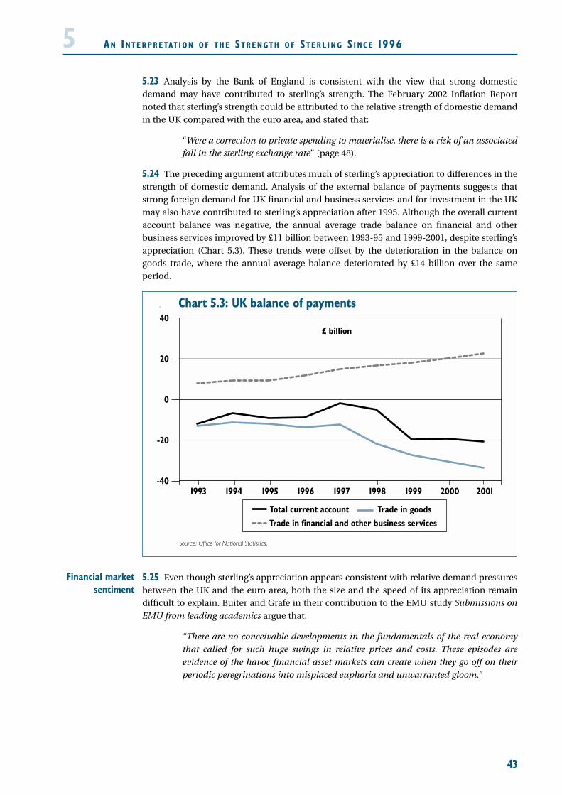
43
5.23 Analysis by the Bank of England is consistent with the view that strong domesticdemand may have contributed to sterling’s strength. The February 2002 Inflation Reportnoted that sterling’s strength could be attributed to the relative strength of domestic demandin the UK compared with the euro area, and stated that:
“Were a correction to private spending to materialise, there is a risk of an associatedfall in the sterling exchange rate” (page 48).
5.24 The preceding argument attributes much of sterling’s appreciation to differences in thestrength of domestic demand. Analysis of the external balance of payments suggests thatstrong foreign demand for UK financial and business services and for investment in the UKmay also have contributed to sterling’s appreciation after 1995. Although the overall currentaccount balance was negative, the annual average trade balance on financial and otherbusiness services improved by £11 billion between 1993-95 and 1999-2001, despite sterling’sappreciation (Chart 5.3). These trends were offset by the deterioration in the balance ongoods trade, where the annual average balance deteriorated by £14 billion over the sameperiod.
5.25 Even though sterling’s appreciation appears consistent with relative demand pressuresbetween the UK and the euro area, both the size and the speed of its appreciation remaindifficult to explain. Buiter and Grafe in their contribution to the EMU study Submissions onEMU from leading academics argue that:
“There are no conceivable developments in the fundamentals of the real economythat called for such huge swings in relative prices and costs. These episodes areevidence of the havoc financial asset markets can create when they go off on theirperiodic peregrinations into misplaced euphoria and unwarranted gloom.”
AN IN T E R P R E TAT I O N O F T H E ST R E N GT H O F ST E R L I N G S I N C E 19965
Chart 5.3: UK balance of payments
Source: Office for National Statistics.
-40
-20
0
20
40
20001999199819971996199519941993 2001
£ billion
Total current account Trade in goodsTrade in financial and other business services
Financial marketsentiment

AN IN T E R P R E TAT I O N O F T H E ST R E N GT H O F ST E R L I N G S I N C E 1996
5.26 As noted in Section 2, the exchange rate is largely determined by expectations of thefuture, which may reasonably switch from euphoria to gloom. Asset market prices areparticularly prone to such swings when there is heightened uncertainty about futureoutcomes. Uncertainty about the relative performance of economies in the longer term willweaken investors’ confidence that a particular exchange rate level is appropriate. In suchcircumstances, financial market sentiment may cause the exchange rate to drift further awayfrom its sustainable level than may appear warranted. This effect may have exacerbatedsterling’s appreciation since 1996.
5.27 The level of the exchange rate is an important element in the overall stance of monetaryconditions, and hence exchange rate movements influence the interest rate decisions of themonetary authorities. For example, Mervyn King, the Deputy Governor of the Bank ofEngland has said3
“although there is little that the MPC can do to influence the exchange rate, it cantake its movements into account when setting interest rates. That it most certainlydoes. Because of the strength of sterling, interest rates have almost certainly beenlower than would otherwise have been the case.”
5.28 As a result the relationship between domestic demand, the exchange rate and interestrates is a complicated mix of underlying developments in supply and demand and, savers’and investors’ expectation of future economic developments in different currency areas,including the expectations of how macroeconomic policy will respond.
Medium-term in f luences on the exchange rate
5.29 To recap, the preceding analysis has suggested that sterling’s strength in recent yearsmay be attributed to the relative strength of demand for UK production compared with euroarea production during this period. This raises two questions:
• Could these trends be purely temporary phenomena?
• If they are permanent, what are the implications for the sustainable exchangerate?
5.30 Medium to long-term explanations of the exchange rate rely on the prediction thatsustained deviations of the exchange rate from its sustainable rate will generate trends thatwill eventually bring the exchange rate back to its equilibrium. But these theories aregenerally unable to predict how rapidly the exchange rate will reach its medium to long-termlevel. This is particularly the case when there is uncertainty about the size and persistence ofthe shifts in supply and demand that are acting to keep the exchange rate away from itslonger-term equilibrium.
5.31 Sterling’s strength over the past few years illustrates these points. Few observersexpected sterling to remain as strong for as long. Nonetheless, this continued strengthcontributed to a steady deterioration in the balance of trade in goods, which has increasinglyacted as a counterweight to the upward pressures on sterling from other sources. This isconsistent with the prediction that prolonged deviations from the medium-term exchangerate will generate trends that help to bring the exchange rate back to its sustainable level.
44
5
Trends takingthe exchange
rate backtowards itsequilibrium
3 Speech entitled “Monetary policy and manufacturing industry”, March 2000. Published on the Bank of England website:www.bankofengland.co.uk.
Monetary policyreaction

45
5.32 These considerations provide a number of explanations for the depreciation of sterlingin early 2003:
• the pressures that contributed to sterling’s appreciation may have themselvesfaded. For example, weaker domestic demand in the UK may have reversedsome of the upward pressure on sterling seen in recent years;
• earlier pressures may still remain, but other pressures may be acting to pushsterling down. So, for example, it could be the case that demand for UKbusiness services remains strong, but demand for sterling relating to othertransactions has weakened; and
• related to the previous point, it may be that the deterioration in the trade ingoods balance, that is in part a consequence of sterling’s previous strength,has become sufficiently strong to outweigh upward pressures from othersources.
5.33 These explanations are not mutually inconsistent, and it may be that each provides partof the total explanation. As always, it is difficult to identify how important each element is,since the underlying influences on currency transactions are not directly observed withsufficient precision. These problems have been exacerbated by the recent high degree ofglobal uncertainty, which has increased the volatility of financial asset markets includingcurrency markets.
5.34 Up until the end of 2002, some argued that sterling’s equilibrium real exchange rate hadappreciated relative to the range of previous estimates. However, sterling’s depreciationduring early 2003 is more supportive of the view that its strength in recent years may havebeen a temporary, albeit protracted, move away from longer-term equilibrium. It is importantto emphasise that interpretation of recent movements is made more difficult by uncertaintiesabout both the scale and persistence of market reactions to the particularly high degree ofglobal political and economic uncertainty.
5.35 Nonetheless, this appreciation may have been warranted by a persistent decrease in netnational saving, associated with relatively strong domestic demand growth in the UKcompared with the euro area. These explanations are considered further in the convergencetest – the first of the Government’s five economic tests for EMU entry.
AN IN T E R P R E TAT I O N O F T H E ST R E N GT H O F ST E R L I N G S I N C E 19965Sterling
depreciation in2003
Implications forthe equilbriumexchange rate

46

6 UK EXC H A N G E RAT E VO L AT I L I T Y
O U T O F O R I N EMU
47
6.1 The analysis in this section attempts to determine the effect on overall UK exchangerate volatility if the UK were to enter EMU. But the analysis comes with a caveat. As theprevious sections have discussed, it is not necessarily the case that any reduction in volatility,either inside or outside of EMU, represents an economic cost or a benefit. If the observedvolatility of the exchange rate is a result of the exchange rate generating an appropriateresponse to an economic shock, then a reduction in volatility is an economic cost. If thisvolatility is an extraneous source of shocks to the economy, then a reduction in volatilityrepresents an economic benefit.
6.2 In practice, observed volatility may be a mixture of both. Effectively, measures ofvolatility conflate ‘warranted’ movements in the nominal exchange rate (that is, movementsof the exchange rate that are an equilibrating response to a fundamental shock) with‘unwarranted’ movements (extraneous movements that do not reflect any change in theunderlying real economy).
6.3 In addition, any reduction in the volatility of nominal variables is also likely to be of littleeconomic benefit if it is not reflected in comparable changes in the behaviour of realvariables.1 If the source of exchange rate volatility is fundamental shocks to the economyrather than extraneous movements then this volatility will manifest itself in the real exchangerate anyway, but not via the nominal rate.
6.4 The handling of exchange rate volatility is also important in studies that attempt toassess the overall macroeconomic cost of entering EMU. Two such recent studies, Barrell andDury (2000) and Minford (2001), arrive at conflicting conclusions largely as a result of theirdiffering treatment of the exchange rate. There is an extended discussion of this issue in theEMU study Modelling shocks and adjustment mechanisms in EMU.
In principle, an exchange rate movement could be an appropriate response of theexchange rate to changing economic conditions or an unwarranted change. In practice,observed volatility may be a mixture of both. Measures of volatility are unable todistinguish between these ‘warranted’ and ‘unwarranted’ exchange rate movements.
If the UK were to join the euro then nominal exchange rate volatility with respect to theeuro area would be eliminated.
In recent times, the euro has been more volatile against the US dollar than sterling hasbeen against the US dollar. If these trends were typical, then the volatility of the UKexchange rate against the US dollar would be higher inside EMU than outside.
In theory, higher volatility against the US dollar might outweigh the effects of eliminatingvolatility against euro area countries.
But this analysis suggests that, in general, increased volatility against the US dollar will notoutweigh the reduction in volatility against euro area currencies. This implies that theoverall volatility of the exchange rate is likely to be lower inside EMU than outside.
1 The earlier discussion in Section 3 examines the possibility of the nominal exchange rate becoming ‘disconnected’ fromthe real economy.
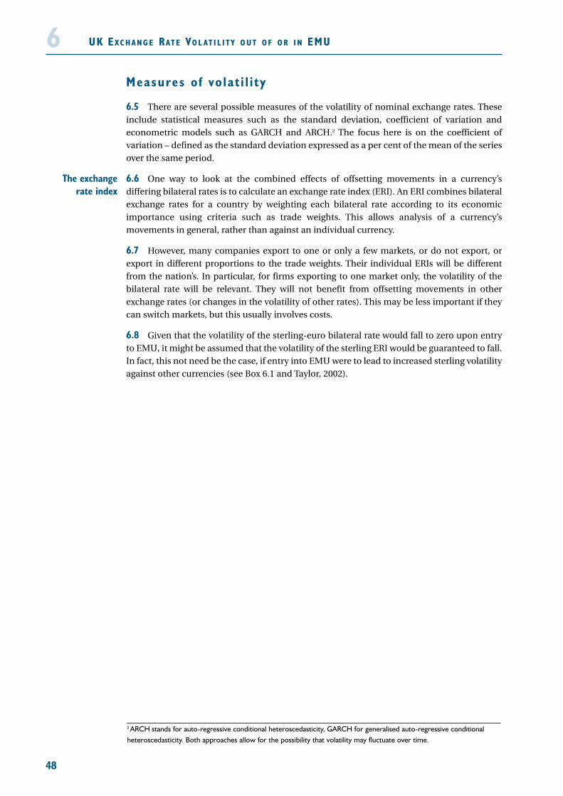
UK EXC H A N G E RAT E VO L AT I L I T Y O U T O F O R I N EMU
Measures o f vo lat i l i ty
6.5 There are several possible measures of the volatility of nominal exchange rates. Theseinclude statistical measures such as the standard deviation, coefficient of variation andeconometric models such as GARCH and ARCH.2 The focus here is on the coefficient ofvariation – defined as the standard deviation expressed as a per cent of the mean of the seriesover the same period.
6.6 One way to look at the combined effects of offsetting movements in a currency’sdiffering bilateral rates is to calculate an exchange rate index (ERI). An ERI combines bilateralexchange rates for a country by weighting each bilateral rate according to its economicimportance using criteria such as trade weights. This allows analysis of a currency’smovements in general, rather than against an individual currency.
6.7 However, many companies export to one or only a few markets, or do not export, orexport in different proportions to the trade weights. Their individual ERIs will be differentfrom the nation’s. In particular, for firms exporting to one market only, the volatility of thebilateral rate will be relevant. They will not benefit from offsetting movements in otherexchange rates (or changes in the volatility of other rates). This may be less important if theycan switch markets, but this usually involves costs.
6.8 Given that the volatility of the sterling-euro bilateral rate would fall to zero upon entryto EMU, it might be assumed that the volatility of the sterling ERI would be guaranteed to fall.In fact, this not need be the case, if entry into EMU were to lead to increased sterling volatilityagainst other currencies (see Box 6.1 and Taylor, 2002).
48
6
The exchangerate index
2 ARCH stands for auto-regressive conditional heteroscedasticity, GARCH for generalised auto-regressive conditionalheteroscedasticity. Both approaches allow for the possibility that volatility may fluctuate over time.

49
The vo lat i l i ty o f s ter l ing compared to other currenc ies
6.9 The first part of this analysis considers the volatility of the bilateral exchange rates ofsterling, the US dollar and the euro, since the latter came into existence in 1999. The analysisthen considers the volatility of major currencies over longer periods.
6.10 Chart 6.1 shows the nominal depreciation of the euro against both the US dollar andsterling since 1999. The weakening of the euro occurred over the first twenty months of itsexistence. For most of the period since then it has been relatively stable against both sterlingand the US dollar, before recently strengthening against both.
UK EXC H A N G E RAT E VO L AT I L I T Y O U T O F O R I N EMU6Box 6.1: Volatility of sterling ERI and covariance
The reason for a possible increase in the sterling ERI after entry to EMU is found in thecovariance of the bilateral exchange rates. The variance of a sum includes a covarianceterm:
Var(aX+bY) = a2Var(X) +b2Var(Y) + 2abCov(X,Y)
As a simple example, assume an ERI comprising only the sterling-US dollar and sterling-euro rates with weights ‘a’ and ‘b’ respectively. This gives:
Var(ERI) = a2Var(£/$) +b2Var(£/A†) + 2abCov(£/$,£/A†)
The assumption that the distribution of shocks would be unaffected by entry to the eurowould imply that the variance of the sterling-euro rate would be zero, the variance of thesterling-US dollar rate would be replaced by the variance of the US dollar-euro rate, andthe covariance term would be zero. Even if the US dollar had a weight equal to that of theeuro, the variance of the US dollar-euro rate would have to be at least twice that of thesterling-euro rate for increased volatility against the US dollar to offset the zero volatilityagainst the euro – unless the covariance between sterling/euro and sterling-US dollar isnegative. In this case, if sterling were to be replaced by the euro, the negative covariancewould drop out of the equation, contributing to a rise in the overall variance.
A negative covariance term implies that when sterling strengthens against either the USdollar or the euro, it tends to weaken against the other. In some sense, sterling would bewalking a stable middle path. This has been the case since the euro was created in 1999.Correlation is a positive function of covariance, and on average the correlation betweenthe sterling-US dollar and sterling-euro rates measured over:
• 60 days was -0.15;
• one year was -0.37; and
• three years was -0.42.
Therefore, replacing sterling with the euro would remove sterling’s ‘bridging’ effectbetween the other two currencies. A later part of this section looks at the rollingcorrelation between the sterling-euro and sterling-US dollar bilateral rates to investigatewhether the negative covariance relationship that has existed since 1999 is a specialfeature of this period or is a more general phenomenon.
Bilateralexchange rates
since 1999
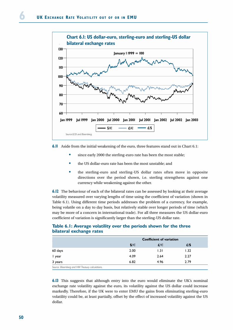
UK EXC H A N G E RAT E VO L AT I L I T Y O U T O F O R I N EMU
6.11 Aside from the initial weakening of the euro, three features stand out in Chart 6.1:
• since early 2000 the sterling-euro rate has been the most stable;
• the US dollar-euro rate has been the most unstable; and
• the sterling-euro and sterling-US dollar rates often move in oppositedirections over the period shown, i.e. sterling strengthens against onecurrency while weakening against the other.
6.12 The behaviour of each of the bilateral rates can be assessed by looking at their averagevolatility measured over varying lengths of time using the coefficient of variation (shown inTable 6.1). Using different time periods addresses the problem of a currency, for example,being volatile on a day to day basis, but relatively stable over longer periods of time (whichmay be more of a concern in international trade). For all three measures the US dollar-eurocoefficient of variation is significantly larger than the sterling-US dollar rate.
Table 6.1: Average volatility over the periods shown for the threebilateral exchange rates
Coefficient of variation
$/A† £/A† £/$
60 days 2.00 1.31 1.32
1 year 4.09 2.64 2.27
3 years 6.82 4.96 2.79Source: Bloomberg and HM Treasury calculations.
6.13 This suggests that although entry into the euro would eliminate the UK’s nominalexchange rate volatility against the euro, its volatility against the US dollar could increasemarkedly. Therefore, if the UK were to enter EMU the gains from eliminating sterling-eurovolatility could be, at least partially, offset by the effect of increased volatility against the USdollar.
50
6
Chart 6.1: US dollar-euro, sterling-euro and sterling-US dollar bilateral exchange rates
Source:ECB and Bloomberg.
60
70
80
90
100
110
120
130
£/$£/€$/€
Jul 2002Jan 2002Jul 2001Jan 2001Jul 2000Jan 2000Jul 1999Jan 1999 Jan 2003
January 1 1999 = 100

51
Ca lcu lat ing an ERI for the UK
6.14 Setting the UK’s exchange rate volatility against the euro to zero and replacing all theother sterling bilateral rates with euro bilateral rates produces the ‘UK-in-euro ERI’. Thissimulates how the UK’s ERI would have moved had the UK been in the euro area since 1999.Contrasting this with the actual sterling ERI shows whether the UK would have experiencedlower exchange volatility had it been a member of the euro area.
6.15 The Bank of England’s official sterling ERI is used for this purpose. This containsweighted bilateral exchange rates between the UK and the euro area, the US, Sweden,Denmark, Norway, Switzerland, Japan, Australia, Canada, and New Zealand. The onlymodification made here is to combine the euro area and Denmark, which has an insignificantimpact on the results.
6.16 An important assumption in this calculation is that the UK’s membership of the euroarea would have influenced the euro-US dollar exchange rate over this period. So the‘constructed’ euro-US dollar exchange rate used in the calculation of the UK-in-euro ERI is acombination of the actual euro-US dollar rate and the actual sterling-US dollar rate weightedby GDP at market prices in value terms. This gives sterling and the euro weights of 18.7 percent and 81.3 per cent, respectively.3
6.17 Chart 6.2 compares the two ERIs for the UK. There are two noteworthy features. First,the actual sterling ERI strengthens through 1999 while the simulated UK-in-euro ERIweakens, which is the result of the general weakening of the euro over that period. Second,the simulated UK-in-euro ERI looks less volatile because there is no longer any exchange ratevolatility with the euro area, which has a weight of 66.5 per cent in the sterling ERI.4
UK EXC H A N G E RAT E VO L AT I L I T Y O U T O F O R I N EMU6
3 These weights are the average of the ratio of UK to euro area GDP in the years 1999-2001.4 Here the euro area includes Denmark.
Chart 6.2: The sterling ERI and simulated UK-in-euro ERI based on Bank of England weights
Source: Bloomberg, Bank of England, HM Treasury calculations.
80
85
90
95
100
105
110
115
120
Sterling ERI UK-in-euro ERI
Jan 1999 Jul 1999 Jul 2001 Jul 2002 Jan 2003Jan 2002Jan 2001Jan 2000 Jul 2000
January 1 1999 = 100

UK EXC H A N G E RAT E VO L AT I L I T Y O U T O F O R I N EMU
6.18 Over the period since the launch of the euro, sterling ERI volatility, measured as thecoefficient of variation, has been 1.96, while UK-in-euro ERI volatility would have been 1.81per cent. However, when volatility is measured over shorter rolling periods the reductions involatility are far more emphatic, as shown in Table 6.2.
Table 6.2: The average of ERI volatility measured over rolling 60 day, 1year and 3 year periods
Coefficient of variation
Simulated
Actual sterling ERI UK-in-euro ERI
60 days 1.00 0.44
1 year 1.52 0.94
3 years 1.67 1.43Source: Bloomberg, Bank of England and HM Treasury calculations.
6.19 According to this simulation, the UK’s overall exchange rate volatility would have beensignificantly reduced had it joined the euro in 1999. This is particularly true for volatilitymeasured over shorter periods.
6.20 This result is consistent with the work of Taylor (2002). This study tested the relationshipbetween sterling and the US dollar to attempt to anticipate the expected fall in sterling’s ERIif the UK were to join EMU. The conclusion was that the UK would benefit from a reductionin high frequency volatility (short run volatility) of about two thirds from joining the euro.However, this finding was also based on using the official ERI weights, which Taylor notes,“may not give a reliable impression of the implications of joining EMU” (page 29).
6.21 Blake and Byrne (2002) use a similar methodology5 to estimate the impact on overallexchange rate volatility of EMU entry. The authors examine the observed relationshipbetween the sterling-US dollar and sterling-deutschmark (euro) rates throughout the last 25years. They note that in the period of floating rates, currencies have tended to simultaneouslyweaken against the US dollar and strengthen against the deutschmark/euro (and vice versa).If this relationship were to remain robust it would offer a clue as to how much the UK in theeuro area would respond to movements in the US dollar.
6.22 The authors conclude that, given the current linkages in currencies’ movements, UKmembership of the euro would lead to increased volatility against the US dollar. However,they go on to suggest that if these currency linkages are dependent on incomes flows, assuggested by Taylor (2002), then “UK membership of the euro could be a help with thereduction of overall currency volatility, and not just the volatility between the UK and thecurrent Euro Area” (Blake and Byrne, 2002, page 45).
6.23 The preceding analysis of ERIs is partly dependent on the assumption made about therelative importance of each currency and its corresponding weight in the ERI calculation. Theissue of how to determine the appropriate weights to use in the ERI is examined extensivelyin Annex B. The following analysis examines the effect of using the alternative weightingsystems discussed there.
52
6
5 This methodology builds on the earlier work of Haldane and Hall (1991).
Using differentweights to
construct theERI

53
6.24 Bootle (2001) uses different weights to construct the ERI, which he argues are morerepresentative of UK trade patterns with other currency areas (see Annex B for more detail).His adjustments reduce the weight of the euro area from just over 66 per cent to less than 47per cent, while increasing the weight of the US dollar from about 16 per cent to over 40 percent. These changes mean that Bootle’s UK-in-euro ERI (shown in Chart 6.3) is more volatilethan the UK-in-euro ERI shown in Chart 6.2. It also depreciates far more during 1999 and2000. This is because the depreciation of the euro against the US dollar during this period isaccorded a greater weight in Bootle’s index than in the official one.
6.25 Applying Bootle’s weights both reduces the volatility of sterling ERI (to 1.77) andincreases the volatility of the UK-in-euro ERI (to 3.47) over the period since the start of EMU.Hence, using these weights implies that, had the UK adopted the euro in 1999, its overallexchange rate volatility since then would have been higher.
6.26 However, as explained earlier volatility measured over the entire period since 1999 doesnot paint a complete picture. When looking at 60-day volatility, on average the differencebetween Bootle’s sterling and simulated UK-in-euro ERIs implies the simulated ERI is actuallymarginally less volatile (around 1 per cent). But, over one-year and three-year periods it is, onaverage, 30 per cent and 48 per cent more volatile respectively.
6.27 It is arguable whether either of the sets of weights used above is appropriate. On nomeasure of trade does the euro area account for over 65 per cent of UK trade. On the basis ofUK current account figures (presented in Annex B), a plausible estimate of the share of UKtrade related to the euro area would be around 55 per cent.6 Assuming the yen accounts foronly 5 per cent, this leaves a substantial share of 40 per cent for the US dollar. So although theimportance of the US dollar stretches well beyond the borders of the US, the euro area is moresignificant for UK trade.
UK EXC H A N G E RAT E VO L AT I L I T Y O U T O F O R I N EMU6
Chart 6.3: The sterling ERI and simulated UK-in-euro ERI based on weights proposed in Bootle (2001)
Source: Bloomberg, Bootle (2001), HM Treasury calculations.
80
85
90
95
100
105
110
115
120
UK-in-euro ERISterling ERI
Jan 1999 Jul 1999 Jul 2001 Jul 2002 Jan 2003Jan 2002Jan 2001Jan 2000 Jul 2000
January 1 1999 = 100
6 Especially assuming that the exchange rates of Central and Eastern Europe are more closely linked to the euro than theUS dollar.
Using a 47 percent euro area
trade share
Using a 55 percent euro area
trade share

UK EXC H A N G E RAT E VO L AT I L I T Y O U T O F O R I N EMU
6.28 Given that a weight of 55 per cent for the euro is between the two previous simulations,the results will also clearly lie between the previous results. The sterling and UK-in-euro ERIsrecalculated using a 55 per cent trade weight for the euro area are shown in Chart 6.4.
6.29 The results from this simulation suggest membership of the euro would have reducedvolatility over the 60-day horizon by about one third and over the one-year horizon by overone tenth (see Table 6.3).7 Over the three-year horizon the estimated volatility from the UKbeing in the euro is about 30 per cent higher than with retaining sterling. But volatility overthe three-year horizon has been on a downward trend, before recently turning upwards again.This can be seen in Chart 6.5.
54
6
Chart 6.4: The sterling and simulated UK-in-euro ERIs calculated with a weight of 55 per cent for the euro
Source: Bloomberg, Bank of England and HM Treasury calculations.
80
85
90
95
100
105
110
115
120
UK-in-euro ERISterling ERI
Jan 1999 Jul 1999 Jul 2001 Jul 2002 Jan 2003Jan 2002Jan 2001Jan 2000 Jul 2000
January 1 1999 = 100
Chart 6.5: Three-year volatility based on ERIs with a 55 per cent euro weighting
Source: Bloomberg, Bank of England, HM Treasury calculations.
0.0
0.5
1.0
1.5
2.0
2.5
3.0
UK-in-euro ERISterling ERI
Mar 2001Jan 2001Nov 2000Sep 2000Jul 2000 Jul 2001May 2001
Coefficient of variation
7 These figures are the average of differences in volatility between the two ERIs.

55
6.30 Table 6.3 summarises the implied impact of euro membership on volatility, using eachof the different trade weights examined above. A negative sign indicates a decrease in thevolatility of sterling ERI upon entry to EMU; a positive sign indicates an increase.
Table 6.3: Impact of euro membership on volatility under different tradeweights
Coefficient of variationSimulated Impact of euro
Sterling UK- membershipERI in-euro ERI on volatility
Bank of England weights 60 days 1.00 0.44 –1 year 1.52 0.94 –
3 years 1.67 1.43 –Bootle (2001) weights 60 days 0.85 0.84 –
1 year 1.34 1.74 +3 years 1.91 2.83 +
55 per cent trade weights 60 days 0.93 0.59 –1 year 1.35 1.27 –
3 years 1.48 1.93 +Source: Bank of England, Bootle, (2001) and HM Treasury calculations.
6.31 The EMU study EMU and trade by HM Treasury considers whether membership of thesingle currency would lead to a substantial increase in trade between the UK and the euroarea, as some studies suggest. Such an effect would increase the weight of the euro area in thesterling ERI, implying that overall exchange rate volatility would be further reduced.
A longer t ime ser ies
6.32 Since the launch of the euro, the US dollar-euro exchange rate has been more volatilethan the US dollar-sterling rate. Furthermore, sterling has generally been stable, following amiddle path between the US dollar and euro, giving a negative correlation between thesterling-euro and sterling-US dollar exchange rates. The question is whether this snapshot isrepresentative of longer-term trends?
6.33 To answer this question it is necessary to use a proxy for the euro. One option is to createan index of the euro legacy currencies; an alternative is to simply use the deutschmark. Usingan index of legacy currencies is consistent with the view that the euro should behave like aweighted average of its component currencies, while using the deutschmark acknowledgesthat euro area institutions are modelled to some extent on their German predecessors. Forcompleteness this study presents both options.
6.34 Chart 6.6 shows the bilateral exchange rates of the US dollar-sterling, US dollar-euro andUS dollar-deutschmark since 1991. Chart 6.7 presents the related one-year measure ofvolatility.
UK EXC H A N G E RAT E VO L AT I L I T Y O U T O F O R I N EMU6
Impact ofmembership of a
currency unionon trade

UK EXC H A N G E RAT E VO L AT I L I T Y O U T O F O R I N EMU
6.35 The US dollar-sterling is the most stable of the three bilateral exchange rates from 1993onwards. The greater volatility seen in 1992 is the result of the UK leaving the ERM. Chart 6.7indicates that the US dollar-deutschmark and US dollar-euro rates were more volatile thanaverage following the start of EMU in 1999. Their volatility then declined over 2000 and 2001before increasing again in 2002.
56
6
Chart 6.6: The US dollar-sterling, US dollar-euro andUS dollar-deutschmark bilateral exchange rates
Source: ECB and Bloomberg.
60
70
80
90
100
110
120
130
$/DM$/€$/£
2001200019991998199719961995199419931991 1992 20032002
January 1 1999 = 100
Chart 6.7: One year bilateral volatility (rolling centred one year coefficient of variation)
Source: ECB and Bloomberg.
0
2
4
6
8
10
12
$/DM$/€$/£
1991 1992 1993 1994 1995 1996 1997 1998 1999 2000 2001 2002
Coefficient of variation

57
6.36 As was noted previously the negative correlation or covariance of the sterling-US dollarand sterling-euro rates seems to have contributed to sterling’s relatively low volatility since1999. However, Chart 6.8 shows that this negative correlation does not hold over all periods inthis longer time series; for example around 1996 and 1997, and post-ERM in 1992, thecorrelation is positive. In these periods sterling was either depreciating or appreciatingagainst both the deutschmark and the US dollar. During such periods membership of EMUwould have entailed a much greater reduction in exchange rate volatility than emerges whenthe simulated volatility is derived using data since 1999.
6.37 Chart 6.9 indicates the sterling ERI and UK-in-euro ERI derived from Bank of EnglandERI weights. The rolling one year volatility of these rates is shown in Chart 6.10.
6.38 The charts indicate that since 1999, sterling has experienced a period of stabilitycompared with the previous years, at least over periods of a year or more. In 1992 sterlingunder went a sharp depreciation on exit from the ERM and a rapid appreciation around 1997.These movements make the post-1999 appreciation against the euro look relatively small incomparison.
6.39 The reverse is true for the UK-in-euro ERI. Had the UK been in the euro in the 1990s, thelarge depreciation and even larger appreciation would not have occurred, so stability wouldhave been improved. But, membership of the euro would also have meant experiencing thefull effects of the euro depreciation against the US dollar in 1999 and 2000.
UK EXC H A N G E RAT E VO L AT I L I T Y O U T O F O R I N EMU6
Chart 6.8: Centred one year rolling correlation between the sterling-US dollar and sterling-euro exchange rates
Source: ECB and Bloomberg.
20012000199919981997199619951994199319921991-1.0
-0.8
-0.6
-0.4
-0.2
0.0
0.2
0.4
0.6
0.8
1.0
2002
Correlation coefficient
ERIs over alonger time
period

6.40 Overall, using Bank of England ERI weights, membership of the euro would haveimplied lower volatility measured over one year windows for the last decade. The effect onthree-year volatility would have been even greater with similar volatility post-1999, butreduced volatility pre-1999.
6.41 Using a greater weight for the US dollar would reduce these differences by reducing thevolatility of the sterling ERI and increasing that of the UK-in-euro ERI, but it would still showthat during the 1990s, the volatility of the UK-in-euro ERI would, on average, have been lowerif sterling had maintained a fixed exchange rate against the euro area currencies.
UK EXC H A N G E RAT E VO L AT I L I T Y O U T O F O R I N EMU
58
6
Chart 6.9: The sterling ERI and UK-in-euro ERI
Source: ECB and Bloomberg.
60
70
80
90
100
110
120
UK-in-euro ERISterling ERI
1991 1992 1993 1995 19961994 19981997 2002 2003200120001999
January 1 1999 = 100
Chart 6.10: Centred one year rolling coefficient of variation
Source: ECB and Bloomberg.
0
1
2
3
4
5
6
7
8
UK-in-euro ERISterling ERI
1991 1992 2001 200220001999199819971996199519941993
Coefficient of variation

59
Conc lus ions
6.42 This section has examined the evidence of the possible effect on the overall volatility ofthe UK’s exchange rate in the event of UK entry to EMU. Measures of volatility need to beinterpreted carefully. To the extent that exchange rate movements aid macroeconomicadjustment, some exchange rate volatility may be useful. But to the extent that exchange ratevolatility disrupts the economy then it may be considered unwarranted. Summary measuresof volatility are unable to distinguish whether observed volatility is warranted or not.
6.43 Since the launch of the euro, the sterling-euro and sterling-US dollar rates have oftenmoved in opposite directions. During this period, the volatility of the US dollar-euro rate hasalso been substantially greater than the sterling-US dollar rate. This suggests that theelimination of sterling volatility against the euro could be offset to some degree by increasedvolatility of sterling against the US dollar.
6.44 That said, the analysis suggests that, in general, overall exchange rate volatility wouldtend to be lower if the UK were to join EMU. But this result varies in different contexts. Thereduction in volatility is greatest in situations where, if sterling were independent, it would bemoving against an unchanged euro-US dollar rate. In these circumstances, fixing the sterling-euro rate not only eliminates volatility against the euro, but also eliminates volatility againstother currencies as well. By contrast, in circumstances of sharp adjustment in the euro-USdollar rate, the overall volatility of sterling might be higher within EMU than outside. Whilesuch circumstances have arisen in the past, and can be expected to arise in the future, theanalysis suggests that more typical scenarios are ones in which the elimination of nominalexchange rate volatility against the euro area would outweigh any increase in sterlingvolatility against non-euro currencies.
UK EXC H A N G E RAT E VO L AT I L I T Y O U T O F O R I N EMU6

60

7 CO N C LU S I O N S : TH E RO L E O F T H E
EXC H A N G E RAT E
61
7.1 This study has considered the question of whether nominal exchange rate flexibilityaids macroeconomic adjustment, both in theory and in practice.
7.2 Optimal currency area theory highlights the conditions in which separate currenciesmay aid adjustment. It demonstrates that separate currencies may be beneficial in securinga real exchange rate change when other adjustment mechanisms, in particular wage andprice adjustment, are sluggish. This is more likely to be the case when economies are notstrongly integrated with each other, since this limits the extent to which price developmentsin one area get transmitted to another, and limits the extent to which resources such aslabour and capital may flow between regions.
7.3 Irrespective of whether a country has its own currency or is part of a currency union,circumstances can arise in which its real exchange rate may need to change in order tomaintain or restore macroeconomic balance. When nominal exchange rates are fixed, realexchange rate adjustment must necessarily come about through differential movements ininflation. That means that if the UK were in EMU, then UK inflation would tend to be higheror lower than the euro area average if a real exchange rate appreciation or depreciation wereneeded. Such changes have already occurred within the existing euro area, where inflationin the Netherlands has been relatively strong while inflation in Germany has been relativelyweak.
7.4 Empirical analysis suggests that exchange rate movements have not been a significantsource of shocks to the UK economy as a whole. Instead, exchange rate changes appear tohave absorbed shocks that might otherwise have had a greater impact on UK output andprices. A striking example of this is sterling’s strong appreciation after 1996, which did notresult in higher unemployment or a collapse in inflation, but nonetheless restrained the netexport contribution to demand and probably alleviated some of the inflationary pressurethat might otherwise have occurred.
7.5 Clearly, exchange rate movements impact more strongly on exporters and importersthan on the economy as a whole, with large exchange rate changes posing particulardifficulties. But the potential benefit of fixed exchange rates to the traded goods sector maybe less than is sometimes claimed. As already noted, real exchange rates can still adjust whennominal rates are fixed, with adjustment coming through movements in relative price levels.Since it is the real exchange rate that influences the price competitiveness of exporters andimporters in their respective markets, they will still find their price competitiveness will tendto rise and fall in response to the strength of economic activity in different markets. Sincedomestic prices tend to move more slowly than exchange rates, companies tend to havemore time to adjust when nominal exchange rates are fixed, but they still remain subject toreal exchange rate changes.
7.6 While nominal exchange rate volatility against other euro area countries would beeliminated if the UK were to join the euro, volatility against other currencies would still bepresent. In recent years the euro has been more volatile against the US dollar than sterlinghas been. If recent trends were to continue then this would offset some, but not all, of thereduction in nominal exchange rate volatility that would arise from fixing the sterling-euroexchange rate.

CO N C LU S I O N S : TH E RO L E O F T H E EXC H A N G E RAT E
62
77.7 Overall, the analysis in this study suggests that movements in the exchange rate moreoften help to stabilise the economy than to destabilise it. Consequently, fixing the euro-sterling exchange rate would remove one of the adjustment mechanisms that is currentlyavailable to the economy. However, the analysis has also highlighted that this need not becostly, provided that other adjustment mechanisms, such as labour market flexibility andfiscal stabilisation operate effectively. These issues are considered further in the convergenceand flexibility tests – the first and second of the Government’s five economic tests for EMUentry.

RE F E R E N C E S
63
Allen, H. and Taylor, M. (1989) ‘Chartists, Noise And Fundamentals: A Study of the LondonForeign Exchange Market’. Centre for Economic Policy Research Working Paper No. 341.
Artis, M. and Ehrmann, A. (2000) ‘The Exchange Rate: A Shock Absorber or Source of Shocks?A Study of Four Open Economies’. Centre for Economic Policy Research Discussion Paper No.2550.
Astley, M. and Garrett, A. (1996) ‘Interpreting Sterling Exchange Rate Movements’. Bank ofEngland Quarterly Bulletin November 1996.
Bailey, A., Millard, S. and Wells, S. (2001) ‘Capital Flows and Exchange Rates’. Bank of EnglandQuarterly Bulletin Autumn 2001.
Balls, E. (2002) ‘Why the five economic tests’ presented at the Cairncross Lecture 2002,available at www.hm-treasury.gov.uk.
Barrell, R. and Dury, K. (2000) ‘Choosing th Regime: Macroeconomic Effects of UK Entry intoEMU’, Journal of Common Market Studies, 30 (4).
Blake, A. and Byrne, J. (2002) ‘Sterling, the Euro and the Dollar’. National Institute EconomicReview No. 181 July 2002.
Blanchard, O (2001) ‘Country adjustments within Euroland: lessons after two years’ inAlesina, A, Blanchard, O, Gali, J, Giavazzi, F and Uhlig, H (eds) Defining a macroeconomicframework for the Euro Area: Monitoring the ECB 3, London: CEPR.
Bootle, R. (2001) ‘Britain’s Trade with the EU and the Rest of the World: What does our CurrentAccount Really Look Like?’ London: New Europe on behalf of the No Campaign.
Breurer, J.B. (1994) ‘An Assessment of the Evidence on Purchasing Power Parity’ inWilliamson, J. (ed) Estimating Equilibrium Exchange Rates. Washington: Institute forInternational Economics.
Buiter, W. (1999) ‘The Clear Case for UK Membership in EMU’, mimeo, Bank of England, June16, 1999.
Buiter, W. (1999a) ‘Optimal Currency Areas: Why Does the Exchange Rate Regime Matter?’,Sixth Royal Bank of Scotland/Scottish Economic Society Annual Lecture, at the Royal Collegeof Physicians, Edinburgh, October 1999. Scottish Journal of Political Economy, Vol. 47, No 3,August 2000, pp. 213-250.
Bush, J. (2001) The economic case against the euro. London: New Europe Campaign.
Campa, J. and Goldberg, L. (2002) ‘Exchange Rate Pass-Through into Import Prices: A Macroor Micro Phenomenon?’. Federal Reserve Bank of New York Staff Reports No. 149.
Campa, J. and Minguez, J. (2002) ‘Differences in Exchange Rate Pass-Through in the EuroArea’. Banco De Espana Working Paper No. 0216.
Cheung, Y., Chinn, M. and Marsh, I. (2000) ‘How do UK-based Foreign Exchange DealersThink their Market Operates?’, National Bureau of Economic Research Working Paper No.7524.
Chinn, M. and Meese, R. (1996) ‘Banking on Currency Forecasts: How Predictable is theChange in Money?’, Journal of International Economics, 38, pp. 161 – 78.

RE F E R E N C E S
Clarida, R. and Gali, J. (1994) ‘Sources of Real Exchange Rate Fluctuations: How Important areNominal Shocks?’, Carnegie-Rochester Series on Public Policy 41, pp. 1-56.
Cobham, D. (2002) ‘The Exchange Rate as a Source of Disturbances: The UK 1979-2000’,National Institute of Economic and Social Research Review, No. 181, July 2002.
Currie, D. (1997) The Pros and Cons of EMU, HM Treasury.
Debelle, G. and Wilkinson, J. (2002) ‘Inflation Targeting and the Inflation Process: SomeLessons from an Open Economy’, Reserve Bank of Australia Research Discussion Paper No.2002-01.
Devereux, M.B and Engel, C. (2002) ‘Exchange Rate Pass-through, Exchange Rate Volatilityand Exchange Rate Disconnect’, National Bureau of Economic Research Working PaperNo. 8858.
Dornbusch, R. (1976) ‘Expectations and exchange rate dynamics’, Journal of PoliticalEconomy, No. 84, pp. 1161-1176.
Eichengreen, B. (1994) ‘History of the International Monetary System: implications forResearch in International Macroeconomics and Finance’ in van de Ploeg, F. (ed.) TheHandbook of International Macroeconomics. Cambridge: Blackwell.
Engel, C. (2001) ‘The Responsiveness of Consumer Prices to Exchange Rates and theImplications for Exchange Rate Policy: A Survey of a Few Recent New Open-Economy MacroModels’, National Bureau of Economic Research Working Paper No. 8752.
European Commission (2001) ‘The EU Economy 2001 Review’, European Economy No. 73.
Flood, R. and Rose, A. (1993) ‘Fixing Exchange Rates: a Virtual Quest for Fundamentals’,National Bureau of Economic Research Working Paper No. 4503.
Flood, R. and Rose, A. (1999) ‘Understanding Exchange Rate Volatility without theContrivance of Macroeconomics’, The Economic Journal, 109, pp. F660-F672.
Friedman, M. (1953) ‘The Case for Flexible Exchange Rates’, in Friedman, M. Essays in PositiveEconomics. Chicago: University of Chicago Press.
Frankel, J. and Froot, K. (1987) ‘Short Term and Long Term Expectations of the Yen/DollarExchange Rate: Evidence from Survey Behaviour’, Journal of the Japanese and InternationalEconomies. No. 1, pp. 249-274.
Frankel, J. and Froot, K. (1990) ‘Chartists, Fundamentalists, and the Demand for Dollars’, inCourakis, A. and Taylor, M. (eds.) Private Behavior and Government Policy in InterdependentEconomies. Oxford: Clarendon Press.
Frankel, J. and Rose, A. (1995) ‘Empirical Research on Nominal Exchange Rates’, in Grossman,G. and Rogoff, K. (eds) The Handbook of International Economics, vol. III. Elsevier Science.
Funke, M. (2000) ‘Macroeconomic Shocks in Euroland vs. the UK: Supply, Demand orNominal?’. University of Hamburg.
Goldberg, P.K. and Knetter, M.M. (1996) ‘Goods Prices and Exchange Rates: What have weLearned?’. National Bureau of Economic Research Working Paper No. 5862
Goodhart, C. (1988) ‘The Foreign Exchange Market: a Random Walk with a Dragging Anchor’,Economica, No. 55, pp. 437-460.
Haldane, H.G. and Hall, S.G. (1991) ‘Sterling’s Relationship with the Dollar and theDeutschmark: 1976-1989’, The Economic Journal, 101, pp. 436-43.
64

65
Huhne, C. and Canning, N. (2002) ‘Crystal Balls: False prophecies from anti-EuropeanEconomists’. London: Britain in Europe.
International Monetary Fund (2002) ‘The rise of the sterling real exchange rate’, UnitedKingdom: Selected Issues, IMF Country Report 02/46, pp. 47-73.
International Monetary Fund (1998) World Economic Outlook. May 1998.
International Monetary Fund (2001) World Economic Outlook. May 2001.
Isard, P. (1995) Exchange Rate Economics. Cambridge: Cambridge University Press.
Ito, T (1994) ‘Short Term and Long Term Expectations of the Yen/Dollar Exchange Rate’,Journal of the Japanese and International Economies, No. 8, pp. 119-143.
Jeanne, O. and Rose, A. (2000) ‘Noise Trading and Exchange Rate Regimes’, Quarterly Journalof Economics, May 2002.
Kara, A. and Nelson, E. (2002) ‘The Exchange Rate and Inflation in the UK’, Monetary PolicyCommittee Unit, Bank of England.
Kenen, P.B. (1969) ‘The Theory of Optimum Currency Areas: An Eclectic View’, in Mundell andSwoboda (eds), Monetery Problems of the International Economy. Chicago: University ofChicago Press.
Krugman, P. (1987) ‘Pricing to Market when the Exchange Rate Changes’ NBER Working PaperNo. 1926.
Krugman, P. (1989) Exchange Rate Instability. Massachusetts: Massachusetts Institute ofTechnology Press.
Labhard, V. and Westaway, P. (2002) ‘What is Shocking Exchange Rates?’, paper presented at2002 EEA meeting in Venice, August.
Layard, R. (2000) The Case for the Euro. London: Britain in Europe Campaign.
Layard, R. (2002) Why Britain should join the Euro. London: Britain in Europe Campaign.
Lyons, R. (1993) ‘Tests of Microstructural Hypotheses in the Foreign Exchange Market’,National Bureau of Economic Research Working Paper No. 4471.
Maclennan, D., Muellbauer, J. and Stephens, M. (2000) ‘Asymmetries in Housing andFinancial Markets and EMU’, Oxford Review of Economic Policy, 14, Autumn, pp. 54 81.
MacDonald, R. (1995) ‘Long-Run Exchange Rate Modelling: A Survey of the Recent Evidence’.IMF Staff Papers, Vol. 42, pp. 437-89.
MacDonald, R. (1999) ‘Exchange Rate Behaviour: Are Fundamentals Important?’, EconomicJournal, No. 109, pp. F673-F691.
Mark, N. (1995) ‘Exchange Rates and Fundamentals: Evidence on Long-horizonPredictability?’, American Economic Review, Vol. 85, pp. 201-18.
McCallum, B.T. and Nelson, E. (2000) ‘Monetary Policy for an Open Economy: An AlternativeFramework with Optimising Agents and Sticky Prices,’ Oxford Review of Economic Policy, 16,pp. 74-91.
McCarthy, J. (2000) ‘Pass-through of Exchange Rates and Import Prices to Domestic Inflationin Some Industrialized Economies’, Federal Reserve Bank of New York Working Paper.
RE F E R E N C E S

RE F E R E N C E S
McKinnon, R.I. (1963) ‘Optimum Currency Areas’, American Economic Review, 53.
McKinnon, R.I. (2002) ‘Optimum Currency Areas and the European Experience’, Economies ofTransition, Vol. 10(2), pp. 343-364.
Meese and Rogoff, K. (1983) ‘The Output of Sample Failure of Empirical Exchange RateModels’, in Frenkel, J. (ed) Exchange Rates and International Macroeconomics. Chicago:University of Chicago Press.
Minford, P. (2001) ‘Tests 1 and 2: Flexibility and the Costs in Economic Variability’, in J. Bush(ed.) The Economic Case Against the Euro.
Mundell, R. (1961) ‘A Theory of Optimum Currency Areas’, American Economic Review, 51,September, pp. 657-65.
Mundell, R. (1973) ‘Uncommon Arguments for Common Currencies’ in Johnson andSwoboda (eds) The Economics of Common Currencies. Allen and Unwin.
Mussa, M. (1990) ‘Exchange Rates in Theory and in Reality’, in Mussa, M. (1990) Essays inInternational Finance No 179, Princeton University.
Nurkse, R. (1944) International Currency Experience: Lessons of the Interwar Period, Geneva:League of Nations.
Obstfeld, M. (2002) ‘Exchange Rates and Adjustment: Perspectives from the New OpenEconomy Macroeconomics’, National Bureau of Economic Research Working Paper No. 9118.
OECD (2002) ‘Economic Survey of the Netherlands’, Paris: OECD.
Rogoff, K. (1997) ‘The Purchasing Power Parity Puzzle’, Journal of Economic Literature, Vol. 34,pp. 647-668.
Rose, A.K. (2000) ‘One Money, One Market: Estimating the effect of Common Currencies onTrade’, Economic Policy, April.
Stockman, A. (1980) ‘A Theory of Exchange Rate Determination’, Journal of Political Economy,Vol. 88, pp. 673-698.
Taylor, C. (2002) ‘Sterling Volatility and European Monetary Union’, National institute ofEconomic and Social Research Discussion Paper No. 197.
Taylor, J. (2000) ‘Low Inflation, Pass-Through and the Pricing Power of Firms’, EuropeanEconomic Review, No. 44.
Taylor, M. (1995) ‘The Economics of Exchange Rates’, Journal of Economic Literature, March1995.
Taylor, M., Peel, D. and Sarno, L. (2001) ‘Non-linear Mean-Reversion in Real Exchange Rates:Toward a Solution to the Purchasing Power Parity Puzzles’, International Economic Review,No. 42(4).
Walton, D. and Broadbent, B. (2003) ‘Can the UK achieve a smooth transition to EMU?’, GlobalEconomics Paper No. 90, Goldman Sachs: London.
Wren-Lewis, S., Westaway P., Soteri S., and Barrell, R. (1991) ‘Evaluating the UK’s choice ofentry rate into the ERM’, Manchester School Money Study Group Conference Volume, 59, pp. 1-22.
66

AAN N E X A : EC O N O M E T R I C AN A LY S I S O FT H E EXC H A N G E RAT E A N DAD J U S T M E N T I N T H E UK EC O N O M Y
67
A1 This annex uses an SVAR model1 developed by HM Treasury to analyse the shocks thathave affected UK economic outcomes over the past twenty years.
A2 The model contains four variables:
• UK GDP;
• UK price level, as measured by the consumer expenditure deflator;
• UK real exchange rate, measured using the IMF measure of normalisedrelative unit labour costs; and
• UK interest rates.
A3 Each of the four variables is regressed on past values of itself and of the other threevariables. Results from these regressions are reported in Table A1.
Table A1: Regression results for SVAR model of the UK economy
Estimation period 1980 Q1 to 2001 Q4
Independent variables Dependent variable
Output Real exchange Interest Inflationgrowth rate change rate rate
Output growth (-1) 0.3376 0.5346 0.0037 -2.7301Output growth (-2) 0.1151 -0.1308 0.0287 0.5782Output growth (-3) 0.1281 -0.6700 0.0406 1.8192
Real exchange rate change (-1) -0.0088 0.2715 -0.0004 -0.2053Real exchange rate change (-2) 0.0100 -0.1011 0.0098 -0.1533Real exchange rate change (-3) -0.0313 0.0275 -0.0053 0.1014
Interest rate (-1) -0.1875 3.3992 1.1772 3.0001Interest rate (-2) -0.4716 -2.8442 -0.3307 -0.5711Interest rate (-3) 0.4911 -0.8199 0.1050 -1.3880
Inflation rate (-1) -0.0038 0.1327 0.0070 -0.4815Inflation rate (-2) 0.0064 0.0591 0.0041 -0.1745Inflation rate (-3) 0.0065 0.0800 0.0060 -0.1996
Constant 2.4488 3.2247 0.0639 1.3068Source: HM Treasury.
A4 The residuals from each regression represent ‘shocks’ to the system, in the sense thatthey are developments that could not be predicted from past observations of the variables inthe system.
A5 By applying appropriate restrictions, it is possible to convert the residuals into‘structural’ shocks that have a clearer economic interpretation. There are a number of waysin which restrictions can be applied, each of which provides differing perspectives on the waythat shocks tend to affect the variables in the model, both initially and in the longer term.
1 SVAR stands for structural vector autoregression. The vector is the four variables estimated in the model,autoregression means that the vector is regressed on its own past values, and the structural element relies on identifyingrestrictions explained in the study.

AN N E X A : EC O N O M E T R I C AN A LY S I S O F T H E EXC H A N G E RAT E A N D AD J U S T M E N T I N T H E UKEC O N O M Y
A6 In this annex, two different identification schemes are used. The first scheme looselyfollows the approach used by Clarida and Gali (1994), and the second loosely follows thatused by Artis and Ehrmann (2000). It turns out that, while the two schemes provide slightlydifferent perspectives on how shocks affect the UK economy, they provide essentially thesame insight into the relation between exchange rate changes and other economic variables.
Clar ida- Gal i s ty le analys is : HM Treasury 1
A7 The first way of analysing the model residuals follows Clarida and Gali (1994) by:
• constraining only one of the four shocks to have a permanent effect on thelevel of output, and denoting this as a supply shock; and
• constraining only one of the remaining three shocks to have a permanenteffect on the level of the real exchange rate. This is labelled demand shock 1.
A8 Demand shock 1 can be thought of as mainly reflecting demand shocks that have adifferent impact on the UK economy than on other countries. Such asymmetric demandshocks may require the real exchange rate to change, whereas common demand shockstypically do not. These shocks are not identical to those identified by Clarida and Gali, sincetheir approach models relative output rather than UK output alone. Hence their supply shockcaptures asymmetric shocks but not symmetric supply shocks, and their demand shockcaptures asymmetric demand shocks. By contrast, the supply shocks in the model used herecapture all permanent supply shocks impacting on the UK, both asymmetric and shared withother countries, while demand shock 1 resembles Clarida and Gali in capturing asymmetricdemand shocks, but may also capture asymmetric supply shocks that affect output in the restof the world but not in the UK. An extension of the model to include rest of the world outputwould enable these supply shocks to be separately identified.
A9 The two remaining shocks cannot, by construction, have any permanent effect on eitherof the two real variables in the model (output and the real exchange rate), but may have apermanent effect on the price level. They may reflect real demand shocks that have asymmetric effect on the UK and other countries, or may reflect nominal shocks. They havebeen labelled demand shocks 2 and 3. These two shocks are separated by constraining one toinclude all interest rate policy reaction, while the other is not associated with an interest ratechange.
A10 This identification scheme implies the following:
• supply shocks may affect all four variables (output, the real exchange rate,interest rate and price level) immediately and may affect output, the realexchange rate and the price level in the long run;2
• demand shock 1 may affect all four variables immediately, but only the realexchange rate and the price level in the long run;
• demand shock 2 may affect all four variables immediately, but only the pricelevel in the long run; and
• demand shock 3 may affect output, the real exchange rate and pricesimmediately, but only the price level in the long run.
68
A
2 The structure of the model implies that there are no permanent effects on either inflation or the real interest rate, andaccordingly no permanent effects on the nominal interest rate.

69
A11 Chart A1 illustrates how each of these shocks affects output, both initially and in thelonger term. In each case a typical shock is applied, to allow a comparison of the relativemagnitude of the impacts of each shock over different time horizons.3 This shows thatdemand shock 2 has most impact on output in the short run, while supply shocks tend tohave a small effect initially, but to accumulate over time. By construction, the three demandshocks have no impact on output in the long run.
A12 Chart A2 illustrates the impact of each shock on the real exchange rate. The fact thatdemand shocks 2 and 3 do not have a long run effect on the level of the real exchange rate isa direct consequence of the restrictions used to derive the shocks. But other features are not.In particular the finding that demand shock 1 tends to have a much larger initial impact onthe real exchange rate than the other shocks is not an imposed feature.
AN N E X A : EC O N O M E T R I C AN A LY S I S O F T H E EXC H A N G E RAT E A N D AD J U S T M E N T I N T H E UKEC O N O M YA
Chart A1: Response of output to different shocks
See text for details of how each shock is derived.Source: HM Treasury.
-0.5
0.0
0.5
1.0
1.5
Demand shock 3Demand shock 2Demand shock 1Supply shock
0 4 8 12 16 20 24 28 32 36 40
Per cent difference from base
Quarters after initial shock
3 Technically, the typical shock is equivalent to the standard error of the derived structural shocks over the whole sampleperiod (1980 to 2001).

AN N E X A : EC O N O M E T R I C AN A LY S I S O F T H E EXC H A N G E RAT E A N D AD J U S T M E N T I N T H E UKEC O N O M Y
70
A
Chart A3: Response of the price level to different shocks
-5
-4
-3
-2
-1
0
1
2
Demand shock 3Demand shock 2Demand shock 1Supply shock
Per cent difference from base
See text for details of how each shock is derived.Source: HM Treasury.
Quarters after initial shock
0 4 8 12 16 20 24 28 32 36 40
See text for details of how each shock is derived.Source: HM Treasury.
Chart A2: Response of the real exchange rate to different shocks
-2
-1
0
1
2
3
4
5
Demand shock 3Demand shock 2Demand shock 1Supply shock
Per cent difference from base
Quarters after initial shock
0 4 8 12 16 20 24 28 32 36 40

71
A13 The price level moves in response to all four shocks, in both the short and long run(Chart A3). The largest short run influences are associated with demand shock 3. Demandshock 1, which is associated with large exchange rate movements typically has less effect onthe price level than the other shocks.
A14 Interest rates tend to move most in response to supply shocks and demand shock 2(Chart A4). As with prices, this suggests that they do not tend to be particularly responsive toexchange rate changes, since the latter are primarily associated with demand shock 1.
A15 An alternative way of analysing these results is to consider the question of how mucheach of the shocks contributes to the unpredictability of the four variables in the model. Thisis done by calculating the contribution each shock makes to the variance of the forecast errorsfor each variable over different time horizons (Chart A5). This illustrates clearly that realexchange rate unpredictability is overwhelmingly associated with demand shock 1. Thisresult is very similar to that found by Clarida and Gali, even though they model the differencebetween UK and foreign output rather than UK output alone.
A16 Demand shock 1 contributes little to the unpredictability of output, the price level orinterest rates. In other words, the shock that typically causes large exchange rate movementstends to have rather moderate effects on other macroeconomic variables.
A17 This analysis suggests that the exchange rate is not a significant source of shocks to theeconomy. It is also consistent with the proposition that the exchange rate may be a significantshock absorber, with movements in the nominal and real exchange rate acting to absorb theimpact of real demand shocks on other variables.
Art is -Ehrmann sty le analys is : HM Treasury 2
A18 The second way of analysing the model residuals follows Artis and Ehrmann (2000) by:
• constraining only one of the four shocks to have a permanent effect on thelevel of output, and denoting this as a supply shock; and
• constraining only one of the remaining three shocks to have an immediateeffect on output. This is labelled demand shock A1. Its properties are that itaccounts for all unexpected changes in output that are not associated withsupply shocks.
A19 The two remaining shocks are defined differently from Artis and Ehrmann. They areseparated by constraining one to include all exchange rate movements. This is labelled anexchange rate shock. As a result of these restrictions, the fourth shock can have no immediateimpact on output or the real exchange rate, but may have an immediate impact on interestrates and the price level. It turns out that it has very little effect on interest rates, andconsequently may be viewed as a price level shock.
AN N E X A : EC O N O M E T R I C AN A LY S I S O F T H E EXC H A N G E RAT E A N D AD J U S T M E N T I N T H E UKEC O N O M YA

AN N E X A : EC O N O M E T R I C AN A LY S I S O F T H E EXC H A N G E RAT E A N D AD J U S T M E N T I N T H E UKEC O N O M Y
72
A
Chart A4: Interest rate response to different shocks
-1.0
-0.5
0.0
0.5
1.0
Demand shock 3Demand shock 2Demand shock 1Supply shock
See text for details of how each shock is derived.Source: HM Treasury.
Quarters after initial shock
Percentage point difference from base
0 4 8 12 16 20 24 28 32 36 40
Chart A5: Contribution of each shock to forecast uncertainty
See text for details of how each shock is derived.Source: HM Treasury.
0
25
50
75
1005 year ahead forecasts1 quarter ahead forecasts
0
25
50
75
100Per cent of forecast error variancePer cent of forecast error variance
Per cent of forecast error variance Per cent of forecast error variance
OutputReal exchange rate
Price level Interest rates
0
25
50
75
1005 year ahead forecasts1 quarter ahead forecasts
0
25
50
75
1005 year ahead forecasts
1 quarterahead forecasts
0
25
50
75
1005 year ahead forecasts1 quarter ahead forecasts
Supply shock Demand shock 1 Demand shock 2 Demand shock 3

73
A20 This identification scheme implies the following:
• supply shocks are identical to the Clarida-Gali scheme considered earlier.Hence they may affect all four variables (output, the real exchange rate,interest rates and the price level) immediately and may affect output, the realexchange rate and the price level in the long run;4
• demand shocks may affect all four variables immediately, but only the realexchange rate and the price level in the long run;
• exchange rate shocks may affect the real exchange rate, the price level andinterest rates immediately, but have no immediate impact on output. In thelong run they only affect the real exchange rate and the price level; and
• price level shocks can only affect the price level and interest ratesimmediately, and only affect the real exchange rate and the price level in thelong run.
A21 Unlike the Clarida-Gali scheme considered earlier, all four shocks have permanenteffects on the real exchange rate (Chart A6). However, the response of the exchange rate shockcaptures most of the variation in the exchange rate, both initially and in the longer term. Inthis respect it closely resembles demand shock 1 analysed earlier. By contrast, demand shockA1 tends to be associated with a more modest movement in the real exchange rate. Thesefindings are similar to those of Artis and Ehrmann.
AN N E X A : EC O N O M E T R I C AN A LY S I S O F T H E EXC H A N G E RAT E A N D AD J U S T M E N T I N T H E UKEC O N O M YA
4 The structure of the model implies that there are no permanent effects on either inflation or the real interest rate, andaccordingly no permanent effects on the nominal interest rate.

AN N E X A : EC O N O M E T R I C AN A LY S I S O F T H E EXC H A N G E RAT E A N D AD J U S T M E N T I N T H E UKEC O N O M Y
74
A
Chart A7: Contribution of each shock to forecast uncertainty
See text for details of how each shock is derived.Source: HM Treasury.
Per cent of forecast error variancePer cent of forecast error variance
Per cent of forecast error variance Per cent of forecast error variance
OutputReal exchange rate
Price level Interest rates
Supply shock Demand shock A1 Exchange rate shock Price level shock
0
20
40
60
80
1005 year ahead forecasts1 quarter ahead forecasts
0
20
40
60
80
1005 year ahead forecasts1 quarter ahead forecasts
0
20
40
60
80
1005 year ahead forecasts1 quarter ahead
forecasts
0
20
40
60
80
1005 year ahead forecasts1 quarter ahead forecasts
Chart A6: Response of the real exchange rate to different shocks
-2
-1
0
1
2
3
4
5
Price level shockExchange rate shockDemand shock A1Supply shock
Per cent difference from base
See text for details of how each shock is derived.Source: HM Treasury.
Quarters after initial shock
0 4 8 12 16 20 24 28 32 36 40
75
A22 Analysis of the contribution of these shocks to forecast uncertainty confirms thatexchange rate shocks account for almost all of the unpredictability in forecasting theexchange rate (chart A7). It also shows that exchange rate shocks contribute very little to theuncertainty in predicting output, the price level or interest rates.
A23 Comparison of Charts A5 and A7 shows that the exchange rate shock derived using theArtis and Ehrmann scheme has very similar properties to demand shock 1 derived using theClarida and Gali approach. In both cases the shock accounts for a high proportion ofexchange rate volatility, but a low proportion of the volatility of other variables. Although theirrespective properties are not identical, they are sufficiently close to suggest that the exchangerate shock in the second scheme could be considered to be demand shock 1 from the firstscheme under a different name.5 Labhard and Westaway (2002) obtain a similar result.
A24 That the two approaches should provide broadly similar results is reassuring andarguably unsurprising. The different approaches provide different perspectives on the samemodel of the UK economy, and it would be more perplexing if they yielded very differentresults.
A25 Both approaches indicate that the shock that causes the real exchange rate to move haslimited effects on other macroeconomic variables. This runs counter to the claim thatexchange rate movements have been a significant source of shocks to the economy, and isconsistent with it acting as a shock absorber.
AN N E X A : EC O N O M E T R I C AN A LY S I S O F T H E EXC H A N G E RAT E A N D AD J U S T M E N T I N T H E UKEC O N O M YA
5 Indeed comparison of Charts A5 and A7 suggests: demand shock 1 in the first scheme broadly resembles the exchangerate shock in the second scheme; demand shock 3 resembles the price level shock; and demand shock 2 resembles,although less closely, demand shock A1. The supply shock is identical in both schemes, by construction.

76

BAN N E X B: DE T E R M I N I N G T H E TR A D E
WE I G H T S T O U S E I N ERICA L C U L AT I O N S
77
B1 Section 6 of this study considers the likely effect on the UK’s overall exchange ratevolatility if the UK were to join EMU. In order to answer this question, a section of theanalysis examines the impact of EMU memebership on a UK-in-euro ERI. This UK-in-euroERI is calculated by combining the bilateral rates for the UK with weights reflecting theimportance of each rate for UK trade. This annex considers the issue of how to determinethese weights.
B2 The EMU study by HM Treasury on EMU and Trade shows that the euro area is the UK’smost important trading partner. Nonetheless, the importance of the euro relative to the USdollar may be overstated by the official exchange rate index. Four factors are important:
• the definition of trade. Specifically, whether income flows from foreigninvestments should be considered;
• the existence of currency blocs. Countries can be assigned to a US dollar,euro or yen currency bloc on the basis of economic or other ties;
• differential regional growth. Relatively slow growth in the euro area meansthat the euro bloc may decline in importance for UK trade; and
• the existence of dollar-standard commodities. Trade in certain goods andservices can also be attributed to the dollar bloc because they are typicallytraded in US dollars.
B3 Two recent studies have considered whether income flows should be taken into accountin the construction of the ERI:
• Bootle (2001) argues that analyses of the importance of different currencyareas should take account of investment income flows as well as flowsgenerated by trade in goods and services. Exchange rate movements affectthe sterling value of UK income from abroad and the foreign currency valueof investment income paid abroad. Therefore, exchange rate movementsaffect the profitability of foreign investment. This plays a role in determiningthe level of foreign investment, and therefore economic activity; and
• Huhne and Canning (2002), by contrast, suggest that income flows areirrelevant when the question under consideration is the effect of exchangerate movements on trade. Furthermore, not all UK income flows are related toactivities that improve economic efficiency. Taylor (2002) notes that UK-based banks intermediating between non-residents give rise to incomecredits and debits in the UK current account that have no real effect.
B4 On balance, it is important to pay attention to income flows when looking at the UK’sinternational exposure, but not so much when looking specifically at trade.
B5 Measures of the ERI often split the world into three currency blocs, with individualcurrencies assigned to a US dollar bloc, euro bloc or yen bloc, depending on the strength oftheir link with these leading currencies. For example, Latin American currencies have closelinks with the US dollar, reflecting the region’s strong trade links with the US.
How importantis UK trade with
the euro area?
Definition oftrade
Currency blocs

AN N E X B: DE T E R M I N I N G T H E TR A D E WE I G H T S T O U S E I N ERI CA L C U L AT I O N S
B6 Bootle (2001) argues that the US dollar bloc could also reasonably include much of Asia,the Middle East and some of Eastern Europe. The euro bloc is then made up of the EU, EFTA1
economies and some African countries with colonial links. Using this broad definition of thetwo blocs, and looking at the current account as a whole, Bootle estimates that 55 per cent ofUK transactions are with the euro bloc. This is slightly lower than the whole of Europe’s sharein the UK current account (see Tables B1 and B2 below). More importantly, this significantlyincreases the size of the US dollar bloc, which Bootle now estimates to account for about 40per cent of UK transactions. The remaining 5 per cent of UK transactions are ascribed to a yenbloc.
B7 This definition of the US dollar bloc includes most of Central and Eastern Europe (CEE).For Russia this may be reasonable, given the reliance of its economy on the oil industry. But forcountries such as the Czech Republic, Poland, Turkey and others, ties with Europe are muchcloser: they are geographically much closer to Europe; there is ongoing integration withexisting EU members; and many of these countries are about to join the EU. Overall, it seemsmore reasonable to regard CEE (excluding Russia) as euro bloc members. According to Bootle’sfigures, this collection of economies accounts for about 4 per cent of UK current accounttransactions.
B8 Tables B1 and B2 provide a geographical breakdown of credits (exports) and debits(imports) for the UK current account averaged over the period 1999 to 2001. It is immediatelyapparent that the euro area, and the EU more generally, is the dominant region with respectto the UK’s international trade. The EU accounts for over half of all UK trade in goods andservices, while the euro area accounts for slightly less than half. For the current account as awhole, the EU is marginally less important but still represents about half of all currentaccount debits and credits. This far exceeds the shares of the US and Asia, which both accountfor less than a fifth of all UK current account transactions.
Table B1: UK current account credits by region, per cent of category total(1999-2001 average)
Goods andTotal services Goods Services Income Transfers
Euro area 45.3 49.1 54.5 36.0 41.1 13.9
add ECB and EU institutions 47.1 49.2 54.5 36.4 41.4 60.2
add rest of EU 50.1 52.7 58.0 39.8 43.7 61.2
add rest of Europe 57.8 60.0 65.0 48.0 52.5 63.0
US 19.1 17.6 15.3 23.3 22.3 18.1
Asia 13.3 13.6 12.3 16.6 13.1 10.6
Other 9.6 8.9 7.7 11.7 11.3 7.9£million, 2001 426,826 267,771 190,050 77,721 142,660 16,395Source: Office for National Statistics.
78
B
The UK currentaccount
1 EFTA is the European Free Trade Association. EFTA economies are Iceland, Liechtenstein, Norway and Switzerland.

79
Table B2: UK current account debits by region, per cent of category total(1999-2001 average)
Goods andTotal services Goods Services Income Transfers
Euro area 42.9 48.8 48.8 48.6 34.5 14.5
add ECB and EU institutions 45.6 48.8 48.8 48.6 35.4 61.1
add rest of EU 48.3 51.9 52.2 50.9 37.5 61.9
add rest of Europe 58.9 60.7 60.9 60.0 53.4 66.1
US 16.3 14.5 13.0 19.5 22.1 7.2
Asia 16.8 17.0 19.0 10.5 17.4 10.4
Other 8.2 7.9 7.4 9.6 7.3 16.6£million, 2001 443,197 290,080 223,659 66,421 130,046 23,071Source: Office for National Statistics.
B9 There are good reasons to think the relative importance of the euro bloc will decline overtime. Developing economies tend to grow faster than developed economies, and most are inthe US dollar bloc. In addition, and notwithstanding recent developments, potential growthin the US itself is still thought to be higher than in Europe.
B10 There are, though, factors working in the opposite direction. Growth in the developingCEE countries is also likely to be relatively high, so pushing up their share of UK trade. Also,ongoing and future integration of CEE with the current EU should further boost UK trade withthese developing countries. In addition, if the UK were to join the euro area, this wouldprovide an additional stimulus to UK trade with the euro area, as discussed in the EMU studyEMU and Trade. More generally, the wealth of the EU and its proximity to the UK means theeuro bloc will remain a very important region for UK trade, even if this importance falls backin the future.
B11 An example of this continuing importance is given in Bootle (2001). Using the morepessimistic of three scenarios, where EU GDP per capita grows at 2.5 per cent per annumcompared to 3 per cent per annum for the rest of the world, Bootle projects that the existingEU will still account for about 33 per cent of UK current account credits in 2050. This is basedon total current account credits, not trade, and ignores the likely enlargement of the EU ormore general economic integration with CEE. Therefore, it is probably fair to assume theimportance of the EU for UK trade will be higher than this figure suggests.
B12 Beyond the country bloc aspects, trade in certain goods is US dollar related. Oil and gasare the obvious examples. The same argument may also apply to IT and pharmaceuticalgoods as well as financial and insurance services. On this basis, Bootle (2001) makes furtheradjustments to his estimates of the size of the euro and US dollar blocs. Assuming that 50 percent of all UK trade in nine product categories2 and seven service categories3 is US dollarrelated boosts the size of the dollar bloc from 40 per cent of UK current account transactionsto about 47 per cent. Equally, the euro bloc share is reduced from about 55 per cent to about47 per cent. On this view, the two blocs are now roughly equal in size.
AN N E X B: DE T E R M I N I N G T H E TR A D E WE I G H T S T O U S E I N ERI CA L C U L AT I O N SB
Differentialregional
economic growth
Dollardenominatedcommodities
2 Inedible crude materials, excluding fuels; Mineral fuels and related materials; Office machines and computers;Telecoms/sound recording apparatus; Professional/scientific instruments; Other transport equipment; Power generatingmachinery and equipment; Other commodity and transactions; and Medicinal and pharmaceutical products.3 Transport; Communication; Insurance; Financial; Computing and information; Royalties; and other business.

AN N E X B: DE T E R M I N I N G T H E TR A D E WE I G H T S T O U S E I N ERI CA L C U L AT I O N S
B13 The assumption that 50 per cent of all UK trade in nine product categories and sevenservice categories is US dollar related can be assessed through UK Customs data. Table B3presents currency of invoicing data by commodity at the SITC4 one-digit level. While an evengreater degree of disaggregation is ideally required, as is data on services, this still shows thatthe US dollar’s share in UK trade was about 50 per cent in only two major categories – crudematerials and mineral fuels and lubricants – and two other less important categories. Moretypically, the US dollar was used as the currency of invoicing for between around 20 and 40per cent of UK trade in the commodities shown.
Table B3: UK trade, invoicing currency by commodity, per cent by value(excludes ‘other’ currencies, which constitute the remainder)
Commodity Sterling euro + DM US Dollar Value (£m)
Food/live animals 56 13 18 20239Beverages and tobacco 70 6 18 7450Crude materials 32 14 48 8851Mineral fuels and lubricants 38 6 53 25671Animal and vegetable oils/fats 16 5 64 707Chemicals 38 16 37 51130Semi manufactures 46 11 39 53943Machinery, transport, misc. manufactures 44 17 29 246011Other commodities 49 0 44 2221Source: HM Customs and Excise 2001 and HMT calculations.
Currency o f invo ic ing
B14 This discussion of US dollar denominated commodities raises more general issuesconcerning the currency used to invoice all trade deals. The currency of invoicing is onlyimportant in the short term while currencies fluctuate around their equilibrium levels, andwhen firms are more likely to be already locked into currency transactions. In the medium tolong term firms can shift the currency they invoice in if volatility is a persistent problem.
B15 In choosing to trade, a firm must make a choice regarding which currency to invoice in.Given the nature of trade, regardless of the currency the firm decides to use, there will have tobe some form of foreign exchange conversion along the way. For example, if a UK firm decidesto invoice in sterling, importers from overseas will have to convert their currency into sterling.If however, UK firms decide to invoice in foreign currency then, assuming they desireultimately to hold sterling, they must convert after the sale.
B16 Conversion of foreign currency is not a costless exercise. Not only is there anadministrative charge on the actual conversion, but holding a foreign currency for any periodof time also creates risks for firms. Hedging is a common method of avoiding risk, although itis not always possible for firms with limited access to capital markets, and hedging itselfimposes costs on the firm.
B17 HM Customs and Excise produce data on the currencies used to invoice UK goods trade.It is important to recognise however, that the coverage of this data is very limited. The samplecovers only 11/2 per cent of all UK goods transactions, and less than 1 per cent of goodstransactions with the EU, and so the figures are likely to vary greatly from year to year.Nevertheless, with this caveat in mind, the figures provide some pointers on invoicingbehaviour.
80
B
4 Standard International Trade Classification.

81
B18 Turning to the data, table B4 unsurprisingly shows that sterling accounts for the greatestshare of UK trade invoices, with US dollars the second most important. Nevertheless, the USdollar is not used in 66 per cent of all UK trade. That said, the US dollar is the most usedcurrency for UK trade with non-EU countries, while the euro is rarely used for this type oftrade. For UK trade with the EU, though, both sterling and the euro are more important thanthe US dollar.
B19 Of course, these figures will partly reflect the euro’s position as a new currency, and itsimportance is likely to increase over time. A recent survey by the Engineering Employers’Federation5 suggested that the euro is now more widely used in UK international trade,overturning the US dollar’s dominance in previous surveys.
Table B4: Currency of invoicing for 2001 (per cent)
Currency EU Non-EU Total
sterling 45 40 42US dollars 18 52 34euro + deutschmark 27 3 16other 10 5 8
Source: HM Customs and Excise.
B20 When interpreting the data it is important to bear in mind that these figures make nodistinction between pricing in a currency and invoicing in a currency. This is best illustratedusing an example.
B21 Consider the situation of a UK exporter and euro area importer where the exporterrigidly prices in US dollars, which means they demand payment of a specified amount of USdollars. The bilateral exchange rates of interest here are the sterling-US dollar and euro-USdollar rates. If the US dollar appreciates against the other two currencies, the exporter gainsand the importer loses, and vice-versa if the US dollar depreciates against the other twocurrencies. If the US dollar moves in opposite directions against sterling and the euro, theneither both parties gain or both parties lose. Given these various possibilities, it seemsunlikely that all traders would enforce rigid pricing in a third currency.
B22 It seems more likely that there will be some flexibility when goods are invoiced in a thirdcurrency, particularly if the firms involved have an ongoing relationship. If one firm gainswhile the other loses from US dollar movements, then they can to some extent agree to offsetthe gains against the losses. An ongoing relationship makes this more likely because the firmswill be aware that at some point in the future the situation could be reversed. Certainly, aflexible approach can prevent the scenario of both firms losing when the US dollar moves inopposite directions against their domestic currencies.
B23 Under this flexible approach to the payment of invoices, the key exchange rate ofinterest is the bilateral sterling-euro rate. While the goods may be invoiced in US dollars,flexible pricing would mean that the sterling-US dollar and euro-US dollar rates are lessrelevant. At the extreme where an exporter only cares about revenue in domestic currencyterms, regardless of whether the US dollar is used for invoicing, the bilateral rate that matterswill be the sterling-euro rate. The same arguments can be applied where trade is invoiced inany third currency. The fact that the US dollar is used in invoicing a substantial proportion ofUK transactions does not necessarily imply that it is much more important than lessfrequently used currencies.
AN N E X B: DE T E R M I N I N G T H E TR A D E WE I G H T S T O U S E I N ERI CA L C U L AT I O N SB
Pricing andinvoicing
5 ‘Manufacturing and the euro – any change?’ Available at<www.eef.org.uk/Downloads/9896DF_Euro%20Survey%20Results%2020021.pdf>

AN N E X B: DE T E R M I N I N G T H E TR A D E WE I G H T S T O U S E I N ERI CA L C U L AT I O N S
B24 It seems clear that the US dollar’s importance exceeds the US share of UK trade orcurrent account transactions. This is because the world can plausibly be thought to containthree currency blocs related to the euro, US dollar and yen. The main points are that:
• the euro bloc perhaps contains all of Europe (excluding Russia) and parts ofAfrica. The US dollar bloc is the rest of the world, excluding Japan;
• the importance of the euro bloc is likely to diminish somewhat because themajority of high potential growth regions of the world are outside of Europe.
• Against this, the EU is likely to enlarge to take in some high potential growthCEE countries and UK trade with the euro bloc countries could receive afurther stimulus if the UK were to join EMU; and
• trade in US dollar-denominated commodities raises the US dollar’simportance further still, though less than some commentators havesuggested. Equally, even where UK trade in invoiced in US dollars, this doesnot necessarily mean that the exchange rate vis-à-vis the US dollar is the mainconcern.
B25 Table B5 below shows the detailed breakdown of the different trade weights used inSection 5.
Table B5: Weights used in the ERIs in Section 5
Bank of England Bootle (2001) 55 per cent weight
Euro area + Denmark 66.53 45.40 55.00Sweden 3.45 1.90 4.64US 16.49 40.85 22.17Japan 7.00 4.10 9.41Norway 1.19 1.20 1.60Switzerland 3.27 3.10 4.40Australia 0.48 1.40 0.66Canada 1.38 1.70 1.86New Zealand 0.21 0.35 0.28Total* 100 100 100Sources: Bank of England and Bootle, 2001.* Final column does not sum to 100 due to rounding error
B26 The official ERI weights are based on guidance from the IMF. For further information onthe calculation of ERIs see the Bank of England Quarterly Bulletin, February 1995 (availableat www.bankofengland.co.uk).
82
BSumming up


