Page 1
TI 2008-041/2 Tinbergen Institute Discussion Paper
The Extent of Internet Auction Markets
Laurens de Haan1,2
Casper G. de Vries2,3
Chen Zhou2,3
1 University of Lisbon; 2 Erasmus University Rotterdam; 3 Tinbergen Institute.
Page 2
Tinbergen Institute The Tinbergen Institute is the institute for economic research of the Erasmus Universiteit Rotterdam, Universiteit van Amsterdam, and Vrije Universiteit Amsterdam. Tinbergen Institute Amsterdam Roetersstraat 31 1018 WB Amsterdam The Netherlands Tel.: +31(0)20 551 3500 Fax: +31(0)20 551 3555 Tinbergen Institute Rotterdam Burg. Oudlaan 50 3062 PA Rotterdam The Netherlands Tel.: +31(0)10 408 8900 Fax: +31(0)10 408 9031 Most TI discussion papers can be downloaded at http://www.tinbergen.nl.
Page 3
The Extent of Internet Auction Markets
Laurens de Haan
Erasmus University Rotterdam and University of Lisbon
Casper G. de Vries ∗
Erasmus University Rotterdam and Tinbergen Institute
Chen Zhou
Erasmus University Rotterdam and Tinbergen Institute
December 10, 2007
Abstract
Internet auctions attract numerous agents, but only a few become active bidders. A
major difficulty in the structural analysis of internet auctions is that the number of potential
bidders is unknown. Under the independent private value paradigm (IPVP) the valuations
of the active bidders form a specific record sequence. This record sequence implies that if
the number n of potential bidders is large, the number of active bidders is approximately
2 log n, explaining the relative inactivity. Empirical evidence for the 2 log n rule is provided.
This evidence can also be interpreted as a weak test of the IPVP.
∗The authors like to thank Alex Koning for his useful comments. We also thank the seminar participants at
the Tinbergen Institute and the University Dordtmund for their remarks. Corresponding author: Casper G. de
Vries, Department of Economics H08-33, Erasmus University Rotterdam, P.O. Box 1738, 3000DR Rotterdam,
The Netherlands. Email: [email protected]
1
Page 4
1 Introduction
Internet auctions (IA) have rapidly become a highly popular mechanism of exchange. The
popularity of IA sites is partly due to the enlargement of the market for rare items. Since
there are only a few buyers and sellers for such goods, creating an easily accessible nation-
wide or global market potentially improves the match between supply and demand. Nev-
ertheless, also many standard commodities, such as notebooks, are sold through online
auction sites. It seems intuitive that a seller is better off the larger is the extent of the
market. Indeed, Bulow and Klemperer (1996) [4] showed that under the hypothesis of the
Independent Private Values Paradigm (IPVP), the seller is better off by enlarging the mar-
ket.1 Similarly, from the buyer’s perspective a larger choice of items and sellers is often the
better.
One of the perhaps surprising facts of IA markets is the low number of active bidders,
notwithstanding the popularity of the mechanism. Consider the well known Ockenfels and
Roth (2002) [11] study of laptop and antiques auctions on eBay and Amazon. This study
covers 120 eBay laptop auctions with 740 active bidders in total and 120 Amazon laptop
auctions with a total of 595 active bidders. This implies an average number of 6.17 active
bidders per auction on ebay and 4.96 active bidders per auction on Amazon. The Bajari
and Hortacsu (2003) [3] study of eBay coin auctions finds 3.08 active bidders on average,
with a standard deviation of 2.51 and a maximum of 14 bidders. As another example, the
study of the online English auction with fixed ending time in Korea by Park and Bradlow
(2005) [13] reports an average number of 5.80 bidders and 8.4 bids per auction.
Most IA sites have two ways of bidding. First, there is the possibility to bid manually,
which is the standard English auction mechanism. Second, the possibility of proxy bidding,
in which a machine bids on behalf of the buyer, adds the Vickrey feature to the auction.
In multiple day English auctions not every manual bidder is continuously active. Some
intervening bids might therefore not materialize, whereas these would be placed under
1But in multi-unit second price auctions entry can lead to lower revenues, see Ausubel and Milgrom (2002) [2].
2
Page 5
proxy bidding. Nevertheless, whatever the exact number of the active bidders is, it is a
rather low number. The potential bidders are those bidders who check the auction website
with or without placing a bid. Potential bidders are in principle interested in buying the
item, but may not be willing to pay the going price. Thus the number of potential bidders
is much larger than the number of actual bidders. We will try to explain the low average
number of active bidders relative to the potential extent of the market.
Consider the number of potential bidders n as the extent of the market. Under the inde-
pendent private value paradigm (IPVP) we show that, under a mild additional assumption,
the valuations of the active bidders forms a sequence of records and second records. By
using the probability theory of records, we then prove that if the number n of potential bid-
ders is large, the number of active bidders is approximately equal to 2 log n. This explains
the relative inactivity, since (2 log n)/n → 0 as n →∞. With this relationship in hand one
can address questions such as by how much the extent of the market has increased through
the creation of IA.
The large amount of data generated by IA is conducive to empirical auction research.
A key difficulty in the analysis of IA data, though, is the fact that the number of potential
bidders is unknown. Many standard auction models require the number of bidders as
a known parameter for identification, see Krishna (2002) [7]. Paarsch (1992) [12] is a
good example of an empirical study in which the number of bidders is known. Several
empirical studies combine the data from multiple auctions to study the IA without knowing
the number of potential bidders for a specific auction. However, this requires an extra
assumption regarding the distribution of the number of bidders. Laffont, Ossard and Vuong
(1995) [8] use the multiple-auctions approach by assuming that the numbers of bidders is the
same across all auctions under consideration. Bajari and Hortacsu (2003) [3] and McAfee
and McMillan (1987) [10] both analyze structural econometric models for multiple auctions
under the assumption that the number of bidders follows a specific stochastic distribution.
Consider the identification problem in auction theory as in Athey and Haile (2002) [1].
Song (2004) [15] discusses this issue for IA and shows that under the IPVP, it is impossible
3
Page 6
to identify the distribution of the bidder’s valuations from the empirical distribution of
bids, without knowing the number of potential bidders, if only the second largest order
statistic is observed. The parent distribution, though, is identified without knowing the
number of potential bidders, when at least two order statistics are observed, i.e. the second
and third largest order statistics. The structural analysis of auctions requires that one can
identify the distribution of valuations from the data under the conjectured equilibrium bid
strategy. The Vickrey mechanism weakly dominant strategies are proxy bids which permit
such identification. But since most IA are a combination of proxy bids and manual bids, an
extra assumption is required for identification. If it can be assumed that manual bidders
respond immediately once they are overbid, this guarantees that their final bid is either the
winning bid, or that it equals their valuation of the item, cf. Song(2004) [15]. Then both
the second and the third largest order statistics can be observed.
While most empirical papers in fact proceed by pooling data across different auctions,
tacitly assuming homogeneity in the distribution of valuations and numbers of potential
bidders, we follow Caserta and de Vries (2005) [5] and study IA on a per auction basis.
But to be able to do this, we need that the number of potential bidders is relatively large.
The 2 log n rule would lend itself easily to empirical scrutiny if the numbers of active and
potential bidders were known. Suppose that the number of page views can be used as an
indicator of potential interest. Fortunately, some smaller sites do report this number. We
will use this information to measure n and to test for the 2 log n rule via regression analysis.
The large IA sites such as eBay and Yahoo! do not record the number of page views and
hence provide no direct information on the number of potential bidders. But information
on the bid arrival time is often publicly recorded. We show that this information can be
used to test the 2 log n rule indirectly, still using the per auction approach, under one extra
maintained assumption. If potential bidders arrive according to a Poisson process, with
a preference for auctions with short remainder time, then the asymptotic property of the
inter arrival times implies the 2 log n rule. We also provide indirect evidence for the 2 log n
rule using these bid arrival times.
4
Page 7
Both the regression evidence and the indirect evidence via the bidding time for the
2 log n rule can be interpreted as a weak test of the IPVP. Alternative settings like common
values and interdependent signals paradigms do not necessarily imply the specific record
sequence which results under the IPVP. Thus insofar the 2 log n rule is not rejected, the
evidence weakly supports the IPVP hypothesis. Notice that most tests of the IPVP contain
several other maintained hypotheses, such as homogeneity across different auctions and the
distribution of the valuations. Here we do not need to maintain these other hypotheses,
except for the assumption regarding the response of the manual bidders in case they are
overbid. But the test is still weak as it only looks at one implication of the auctions under
IPVP and the alternative paradigms do not necessarily destroy the 2 log n rule, so that the
alternative hypothesis is not well specified. In Bajari and Hortacsu (2003) [3] the IPVP
is tested versus the common value pardigm by means of the winner’s curse, which is more
severe the larger the number of bidders. For rare coin auctions the common value paradigm
is the natural null hypothesis as is pointed out by Bajari and Hortacsu. In this paper we
focus on laptops which a priory better fits the IPVP.
The paper is organized as follows. In Section 2, we review certain aspects of IA. Identi-
fication strategies are discussed in Section 3. Section 4 discusses bids as a record sequence.
Our main theorem in Section 5 gives the asymptotic distribution of the index of the record
sequence. Section 6 discusses the empirical evidence of the 2 log n rule via the number of
pageviews. Simulations and empirical evidence for the 2 log n rule via the timing of the bids
are provided in Section 7. Section 8 concludes. Proofs are relegated to the Appendix A. An
example clarifying some notation in the paper is given in Appendix B.
2 The Online Auction
In comparison to offline auctions, the IA exhibit three main differences: the bidding system,
the termination rule and the reminder system. We discuss these features in the following
three subsections.
5
Page 8
2.1 The bidding system
IA sites usually permit a choice between alternative bid procedures. Most common is the
choice between manual and proxy bidding. For a manual bid, the bidder just enters an
amount higher than the currently prevailing price. Manual bidding is like the first price
open ascending bid in an English auction. The system immediately places the bid at the
amount which is entered. A proxy bidder (secretely) communicates the maximum amount
he is willing to bid to the server of the auction site, after which the machine takes over the
bidding for this bidder. The proxy bidding procedure captures the second price sealed bid
mechanism studied by Vickrey (1962). Thus, if the newly entered manual bid is below the
maximum willingness to pay of one previous proxy bidders, the system will raise the price
to the minimum increment above the newly entered manual bid. Otherwise the manual
bid becomes the currently prevailing price. Similarly, a new proxy bidder may find that
he is immediately outbid by another proxy bidder. When two proxy bids are placed, the
current price will automatically jump to the lower of the two maximum willingness to bid
submissions plus the smallest possible increment.
2.2 The termination rules
There exist broadly two alternative termination rules. Either the auction ends after a pre-
announced fixed lapse of time, or there is variable termination time. On eBay, the auctions
have a fixed ending time. The winner is the highest bidder at the time of the close. Per
contrast, Amazon type auctions use an auto-extension termination rule. Before the auction
starts an initial ending time is announced. If no bidding takes place during the last ten
minutes, the auction stops at the initial pre-announced time. But if there are some bids
in the last ten minutes, the ending time is automatically extended by another ten minutes.
This rule is also applied to the new extension period. Thus the auction will only end once
no bidding activity has occurred within the last ten minutes before the previous ending
time, otherwise, the ending time is extended automatically. On the Yahoo! auction site the
sellers can choose which of the two termination rules they adopt.
6
Page 9
The influence of the different termination systems on the bidding strategy is considerable.
The fixed ending time on eBay invites strategic last minute bidding, called sniping. This
avoids competition, since other bidders may be unable to respond due to a lack of time, see
Ockenfels and Roth (2003) [11]. In the Amazon-style auction sniping is not observed.
2.3 The reminder system
Most IA sites have an email based reminder system to inform active bidders about the fact
that they are outbid. This is particularly relevant for those active bidders who use the
manual system. Since many of these auctions run for several days or even longer, those
agents may rely on such automated signalling before becoming active again. With the
reminder system, the IA for the manual bidder in effect becomes a continuous open English
auction. But note that the English auction under the IPVP is strategically equivalent
to a second price auction. Most IA sites go through great pains in trying to explain this
equivalence, so that bidders are stimulated to use the proxy bidding. But given the strategic
incentives for sniping with the fixed ending time, manual bidding is nevertheless often
observed. Moreover, for items like collectibles for which the IPVP may not be appropriate,
manual bidding may again be preferable for strategic reasons.
3 Maintained Hypothesis
Before we can come to the main theme of the paper, we first have to ascertain that the
bid sequence is revealing with respect to the valuations. To analyze this issue for IA, first
consider a hypothetical IA on which only the proxy bidding mechanism is available and to
which the Amazon termination rule applies. Under the IPVP the weakly dominant strategy
is to bid one’s valuation. If bidders act in this way, each active bidder’s valuation will be
observed as his last bid, except for the winner.
Next, consider the hybrid IA with the possibility of manual bidding added to the proxy
bidding mechanism. To ensure that the third largest and lower valuations are observed as
7
Page 10
actual bids in the case with manual bidding, we use an assumption introduced by Song
(2004) [15] for identification of the third largest valuation. Suppose that when the third
highest valuation bidder is overbid, he is immediately notified by the reminder system if he
is bidding manually. This enables the manual bidder to respond directly. We will assume
that the manual bidder indeed immediately counters with a higher bid as soon as he is
overbid and as long as his valuation is above the current price. This assumption ensures
that his valuation is observed as the second highest bid once the auction has terminated.
In this paper the analysis is in principle concluded on a per auction basis, i.e. we do not
necessarily pool across different auctions by making homogeneity assumptions. To enable
this analysis, we therefore like to use the bids from bidders other than the top three, to
increase the information content. For this reason, we will assume that all the (active)
manual bidders immediately respond to a counter bid:
Assumption 3.1. Each active (manual) bidder immediately returns to the IA and increases
his bid as soon as he is overbid and his valuation is above the prevailing price.
We already noted that Assumption 3.1 is automatically satisfied when there are only
proxy bidders present. For the manual bidders, as we discussed in section 2.2, they may
have an incentive to bid later when there is a fixed ending time. However, with the Amazon
style auction termination rule, the active bidders (both proxy bidder and manual bidder)
have no incentive to wait. In this case, the assumption provides a lower bound to the
number of active bidders. Without an immediate response, some other manual bids might
intervene, whereas these would not be placed in the case Assumption 3.1 applies.
Given the Assumption 3.1, the currently prevailing price must be equal to the second
highest valuation among all the potential bidders up to that moment. Therefore the current
price faced by a new potential bidder must be the second highest valuation among all the
potential bidders who were actively bidding earlier on. Hence, in order to motivate a
new potential bidder to bid, his valuation must be higher than the current second highest
valuation. This conclusion is summarized in the first proposition.
8
Page 11
Proposition 3.1. Consider an IA with a hybrid system of manual and proxy bids. Suppose
that Assumption 3.1 within the IPVP setting applies, then each active bidder’s valuation
is the highest or second-highest among all the valuations of the potential bidders who were
active before.
4 Bids as a specific Record Sequence
Proposition 3.1 implies that the bids can be viewed as records of the valuations of the
potential bidders. The sequence of bids constitutes a quite particular record sequence, which
we can characterize. There exists a well developed theory of records in probability theory,
see the book by Resnick (1987) [14]. This theory will be used to derive the novel 2 log n
rule. We first introduce the concept record and 2-record sequence. Let i = 1, 2, · · · , n denote
the order in which the n potential bidders check the auction site. Suppose the valuation of
all potential bidders are i.i.d. random variables X1, X2, · · · , Xn with distribution function
F (x). Define the rank sequence {Ri}ni=1 as
Ri :=i∑
k=1
1{Xk≥Xi}, (1)
where Ri is the rank of the valuation of the i−th potential bidder among the valuations of
all the potential bidders who checked the auction before agent i. The valuation Xi is called
a record if Ri = 1. Similarly, it is a 2-record if Ri = 2. Denote the indices of the records
and 2-records as {J(j)}mj=1. This index sequence is given by
J(1) = 1, J(2) = 2 (2)
J(j + 1) = min {i > J(j) : Ri ≤ 2} , j = 2, 3, · · · ,m− 1, (3)
where m is the number such that Ri > 2 for all i > J(m), i.e. m is the number of active
bidders. Then, the active bidders’ valuations constitute the record and 2-record sequence
{XJ(j)
}m
j=1. An example to clarify the notation is presented in Appendix B.
Under Assumption 3.1, from Proposition 3.1 we get the following corollary.
9
Page 12
Corollary 4.1. Under Assumption 3.1, the active bidders’ valuations are{XJ(j)
}m
j=1. If
an active bidder is not the winner, his valuation is observed as his last bid.
5 Main Theorem
Corollary 4.1 implies that the record and 2-record sequence is{XJ(j)
}m
j=1. Our main
theorem studies the property of the index sequence {J(j)}. The proof is relegated to
Appendix A.
Theorem 5.1. As the number of potential bidders n → ∞, the number of active bidders
m → ∞ as well. Given that k → ∞, the sequence {log J(k + j)− log J(k + j − 1)}∞j=1 is
asymptotically an i.i.d sequence with exponential distribution and mean 1/2.
Remark 5.1. In fact, based on the record and 2-record sequence, one can prove–in a way
analogous to the proof of Corollary 4.5 of Resnick (1987) [14] for the record sequence–that
the point process with points
{12
log J(j)− 12
log n
}∞
j=1
converges to a homogeneous Poisson point process. However, our proof of Theorem 5.1 is
not based on point processes, and follows a simpler and novel approach.
Intuitively, Theorem 5.1 states that the differences of the sequence log J(j) are asymp-
totically i.i.d. and have an exponential distribution with mean 1/2. This indicates that
log J(m) is approximately m/2 for sufficiently large m. Note that m active bidders will be
observed until there are J(m) potential bidders; conversely, one could say that if there are
n potential bidders, the number of active bidders will be approximately 2 log n.
We make this result precise by studying the asymptotic behavior of J(m). To this end
we first need to introduce two more sequences of random variables:
ξi = 1{Ri≤2}, and N(i) =i∑
k=1
ξk. (4)
The number {ξi} indicates whether the i−th potential bidder is an active bidder or not.
10
Page 13
The sequence {N(i)} gives the number of active bidders among the first i potential bidders.
An example of these two other sequences is also shown in Appendix B.
The following two lemmas study the asymptotic normality of both the N(n) and J(m)
sequences. The proofs are given in Appendix A.
Lemma 5.1. With the notation N(n) defined in (4), the sequence
N(n)− 2 log n√2 log n
is asymptotically standard normal, as n →∞.
Lemma 5.2. The sequence
2 log J(m)−m√m
is also asymptotically standard normal, as m →∞.
These lemmas imply the following convergence (in probability) results. As n → ∞
and/or m →∞, we have that
N(n)2 log n
P−→ 1 and2 log J(m)
m
P−→ 1. (5)
Notice that N(n) is the number of active bidders, while n is the number of potential bidders.
Conversely, J(m) is the number of potential bidders when we do observe m active bidders.
Thus (5) gives the asymptotic relationship between the two sequences. This yields the
2 log n rule.
Rule 5.1 (2 log n). If the number of potential bidders n is large, the number of active bidders
is approximately equal to 2 log n.
The 2 log n rule relates the extent of the IA as measured by n to the market activity as
measured by the number of active bidders N(n). In the empirical sections we will test for
this rule.
The 2 log n-rule has implications for the time sequence of the bids in Amazon type
auctions. Define the time at which a record or second record occurs as the entering time.
Obviously, the entering time is related to the index sequence {J(j)}mj=1. Note that most
11
Page 14
auction sites do report the timing of the bids, but do not report the number of page views
as an indicator of the number of potential bidders. Therefore a direct test of the 2 log n
rule is not possible with publicly available data on such kind of auction sites. An indirect
test may be feasible, however, by using the entering time sequence of the records. To see
this, we model the arrival process of the potential bidders. The simplest model is the
homogenous Poisson arrival process. Under Poisson arrivals, the appearance of potential
bidders is random from the viewpoint of the seller and is independent from the time the
auction has been running. Since we consider Amazon type auctions, there is no strategic
reason for late bidding, but bidders may nevertheless display a preference for auctions which
are close to the end of their run times. Most auction sites offer the possibility to easily rank
order the relevant auctions on the remaining time to the announced deadline. Suppose
agents actively use this feature for selecting auctions which are soon to close. Everything
else equal, this preference arises from the cost of having to wait until the end of the auction.
Therefore, we assume that the Poisson arrival rate λ increases as time progresses according
to the following function
λ(t) = λ0eθt, (6)
where θ is the time preference factor, and where the beginning of the auction is at t = 0. Re-
versing time, θ can also be seen as the discount factor under continuous discounting. Since
the Amazon type auction can be extended, we do not specify the end time. The time prefer-
ence turns the homogenous Poisson arrival process into a non-homogeneous Poisson process
with the instantaneous arrival rate λ(t), see, for example, Klein and Roberts (1984) [6].
For this non-homogeneous Poisson arrival process, we derive the asymptotic form of the
entering time process of the record and 2-record sequence. The result is presented in the
following theorem. The proof of the theorem is again relegated to Appendix A.
Theorem 5.2. Suppose the potential bidders 1, 2, · · · , n arrive at times T (1), T (2), · · · , T (n).
Let {T (i)}∞i=1 be the arrival times of a non-homogeneous Poisson process where the rate of
occurrence function is given as in (6). Then the arrival times of the active bidders is
12
Page 15
{T (J(j))}mj=1. For l → ∞, the sequence {T (J(l + j))− T (J(l + j − 1))}∞j=1 is asymptoti-
cally an i.i.d sequence with exponentially distributed innovations that have mean 1/(2θ).
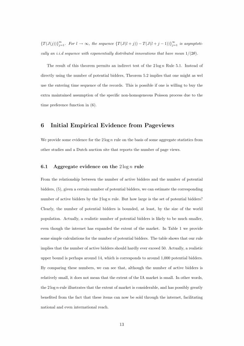
The result of this theorem permits an indirect test of the 2 log n Rule 5.1. Instead of
directly using the number of potential bidders, Theorem 5.2 implies that one might as wel
use the entering time sequence of the records. This is possible if one is willing to buy the
extra maintained assumption of the specific non-homogeneous Poisson process due to the
time preference function in (6).
6 Initial Empirical Evidence from Pageviews
We provide some evidence for the 2 log n rule on the basis of some aggregate statistics from
other studies and a Dutch auction site that reports the number of page views.
6.1 Aggregate evidence on the 2 log n rule
From the relationship between the number of active bidders and the number of potential
bidders, (5), given a certain number of potential bidders, we can estimate the corresponding
number of active bidders by the 2 log n rule. But how large is the set of potential bidders?
Clearly, the number of potential bidders is bounded, at least, by the size of the world
population. Actually, a realistic number of potential bidders is likely to be much smaller,
even though the internet has expanded the extent of the market. In Table 1 we provide
some simple calculations for the number of potential bidders. The table shows that our rule
implies that the number of active bidders should hardly ever exceed 50. Actually, a realistic
upper bound is perhaps around 14, which is corresponds to around 1,000 potential bidders.
By comparing these numbers, we can see that, although the number of active bidders is
relatively small, it does not mean that the extent of the IA market is small. In other words,
the 2 log n-rule illustrates that the extent of market is considerable, and has possibly greatly
benefited from the fact that these items can now be sold through the internet, facilitating
national and even international reach.
13
Page 16
Number of potential bidders (n) 6 billion 1 million 10,000 5,000 1,000 500 100
Estimates of active bidders (2 log n) 49.64 27.63 18.42 17.03 13.81 12.43 9.21
Standard deviation (√
2 log n) 7.05 5.26 4.29 4.13 3.72 3.53 3.03
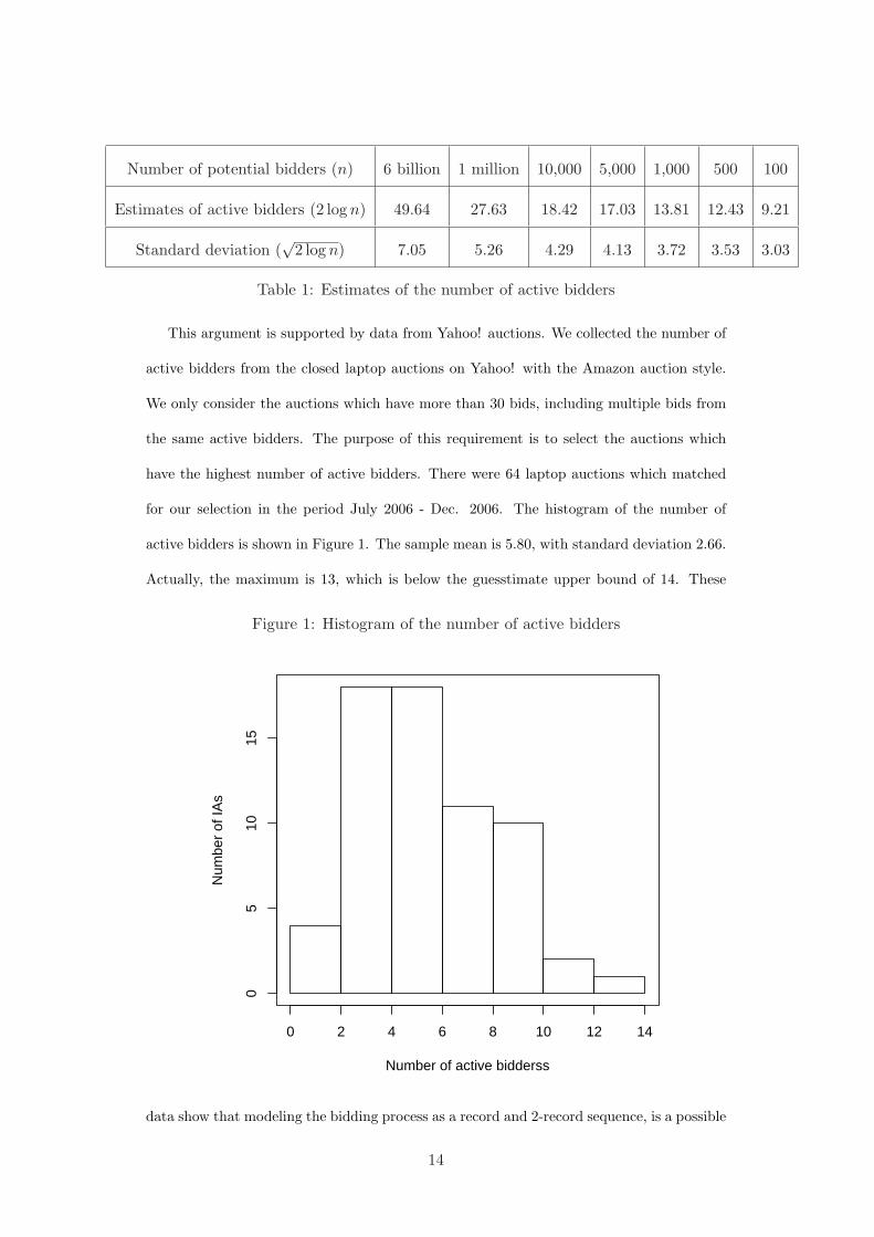
Table 1: Estimates of the number of active bidders
This argument is supported by data from Yahoo! auctions. We collected the number of
active bidders from the closed laptop auctions on Yahoo! with the Amazon auction style.
We only consider the auctions which have more than 30 bids, including multiple bids from
the same active bidders. The purpose of this requirement is to select the auctions which
have the highest number of active bidders. There were 64 laptop auctions which matched
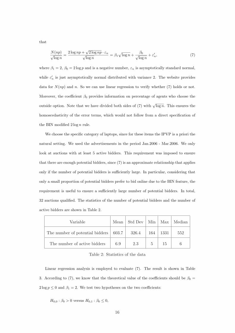
for our selection in the period July 2006 - Dec. 2006. The histogram of the number of
active bidders is shown in Figure 1. The sample mean is 5.80, with standard deviation 2.66.
Actually, the maximum is 13, which is below the guesstimate upper bound of 14. These
Figure 1: Histogram of the number of active bidders
Number of active bidderss
Num
ber
of IA
s
0 2 4 6 8 10 12 14
05
1015
data show that modeling the bidding process as a record and 2-record sequence, is a possible
14
Page 17
explanation for why there are mostly few active bidders participating in a specific IA.
6.2 Regression evidence on the 2 log n rule
On the large IA websites of eBay, Amazon and Yahoo!, the number of potential bidders is
not reported. This hampers a direct evaluation of the 2 log n rule. Fortunately, on some
websites a system is in place that reports the number of people who checked a specific
webpage. Potential bidders are identified uniquely by their IP addresses. In this way we
are able to record the number of potential bidders. For example, the eBay owned Dutch
advertising website www.marktplaats.nl (denoted as Marktplaats in the rest of this paper)
reports such kind of data. This creates a possibility to verify the model by (5).
Marktplaats is an advertising site with the option to bid or to negotiate. The auction is
of the Amazon variety without a termination rule. Moreover, bids are non-binding as the
bidder and seller have to finalize their agreement through an email contact. The website has
the additional Buy It Now (BIN) feature that gives the bidders the possibility to contact
the seller directly via email to bargain over the price. In contrast to several other sites
with the BIN feature, it does not come with a posted price. Instead, the BIN feature is
of the bargaining variety in which the buyer can make an email offer that can be accepted
or countered by the seller. One of the attractions of an auction is that it reduces the
transactions cost in the sense that it cuts out direct negotiations between the seller and the
potential buyers. Thus a percentage of buyers can be expected to prefer not to enter into
the costly process of bargaining, while some others, including the seller, may be tempted
into bargaining.
Assume that there is a fixed percentage p of pageviewer who want to proceed by placing
a bid. It means that, if there are n potential bidders, there will be only np who consider
to place a bid on website, while the others choose the outside option to directly approach
the seller. The number of active bidders therefore reads N(np). From Lemma 5.1, we have
15
Page 18
that
N(np)√log n
=2 log np +
√2 log np · εn√
log n= β1
√log n +
β0√log n
+ ε′n, (7)
where β1 = 2, β0 = 2 log p and is a negative number, εn is asymptotically standard normal,
while ε′n is just asymptotically normal distributed with variance 2. The website provides
data for N(np) and n. So we can use linear regression to verify whether (7) holds or not.
Moreover, the coefficient β0 provides information on percentage of agents who choose the
outside option. Note that we have divided both sides of (7) with√
log n. This ensures the
homoscedasticity of the error terms, which would not follow from a direct specification of
the BIN modified 2 log n rule.
We choose the specific category of laptops, since for these items the IPVP is a priori the
natural setting. We used the advertisements in the period Jan.2006 - Mar.2006. We only
look at auctions with at least 5 active bidders. This requirement was imposed to ensure
that there are enough potential bidders, since (7) is an approximate relationship that applies
only if the number of potential bidders is sufficiently large. In particular, considering that
only a small proportion of potential bidders prefer to bid online due to the BIN feature, the
requirement is useful to ensure a sufficiently large number of potential bidders. In total,
32 auctions qualified. The statistics of the number of potential bidders and the number of
active bidders are shown in Table 2.
Variable Mean Std Dev Min Max Median
The number of potential bidders 603.7 326.4 164 1331 552
The number of active bidders 6.9 2.3 5 15 6
Table 2: Statistics of the data
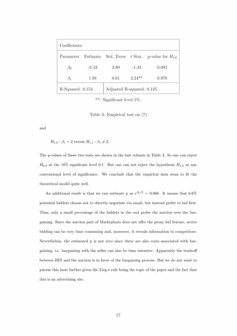
Linear regression analysis is employed to evaluate (7). The result is shown in Table
3. According to (7), we know that the theoretical value of the coefficients should be β0 =
2 log p ≤ 0 and β1 = 2. We test two hypotheses on the two coefficients:
H0,0 : β0 > 0 versus H0,1 : β0 ≤ 0,
16
Page 19
Coefficients:
Parameter Estimate Std. Error t Stat. p-value for Hi,0
β0 -5.43 3.80 -1.43 0.082
β1 1.98 0.61 3.24** 0.970
R-Squared: 0.153 Adjusted R-squared: 0.125
**: Significant level 5%.
Table 3: Empirical test on (7)
and
H1,0 : β1 = 2 versus H1,1 : β1 6= 2.
The p-values of these two tests are shown in the last column in Table 3. So one can reject
H0,0 at the 10% significant level 0.1. But one can not reject the hypothesis H1,0 at any
conventional level of significance. We conclude that the empirical data seem to fit the
theoretical model quite well.
An additional result is that we can estimate p as eβ0/2 = 0.066. It means that 6.6%
potential bidders choose not to directly negotiate via email, but instead prefer to bid first.
Thus, only a small percentage of the bidders in the end prefer the auction over the bar-
gaining. Since the auction part of Marktplaats does not offer the proxy bid feature, active
bidding can be very time consuming and, moreover, it reveals information to competitors.
Nevertheless, the estimated p is not zero since there are also costs associated with bar-
gaining, i.e. bargaining with the seller can also be time intensive. Apparently the tradeoff
between BIN and the auction is in favor of the bargaining process. But we do not want to
pursue this issue further given the 2 log n rule being the topic of the paper and the fact that
this is an advertising site.
17
Page 20
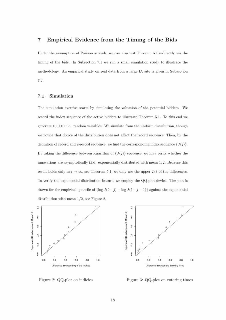
7 Empirical Evidence from the Timing of the Bids
Under the assumption of Poisson arrivals, we can also test Theorem 5.1 indirectly via the
timing of the bids. In Subsection 7.1 we run a small simulation study to illustrate the
methodology. An empirical study on real data from a large IA site is given in Subsection
7.2.
7.1 Simulation
The simulation exercise starts by simulating the valuation of the potential bidders. We
record the index sequence of the active bidders to illustrate Theorem 5.1. To this end we
generate 10,000 i.i.d. random variables. We simulate from the uniform distribution, though
we notice that choice of the distribution does not affect the record sequence. Then, by the
definition of record and 2-record sequence, we find the corresponding index sequence {J(j)}.
By taking the difference between logarithm of {J(j)} sequence, we may verify whether the
innovations are asymptotically i.i.d. exponentially distributed with mean 1/2. Because this
result holds only as l →∞, see Theorem 5.1, we only use the upper 2/3 of the differences.
To verify the exponential distribution feature, we employ the QQ-plot device. The plot is
drawn for the empirical quantile of {log J(l + j)− log J(l + j − 1)} against the exponential
distribution with mean 1/2, see Figure 2.
0.0 0.2 0.4 0.6 0.8 1.0
0.0
0.2
0.4
0.6
0.8
1.0
Difference Between Log of the Indices
Exp
onen
tial D
istr
ibut
ion
with
Mea
n 1/
2
Figure 2: QQ-plot on indicies
0.0 0.2 0.4 0.6 0.8 1.0
0.0
0.2
0.4
0.6
0.8
1.0
Difference Between the Entering Time
Exp
onen
tial D
istr
ibut
ion
with
Mea
n 1/
2
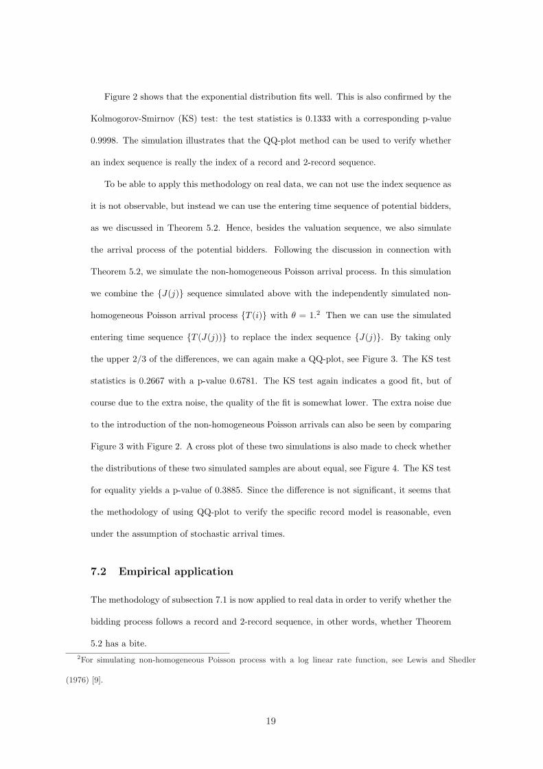
Figure 3: QQ-plot on entering times
18
Page 21
Figure 2 shows that the exponential distribution fits well. This is also confirmed by the
Kolmogorov-Smirnov (KS) test: the test statistics is 0.1333 with a corresponding p-value
0.9998. The simulation illustrates that the QQ-plot method can be used to verify whether
an index sequence is really the index of a record and 2-record sequence.
To be able to apply this methodology on real data, we can not use the index sequence as
it is not observable, but instead we can use the entering time sequence of potential bidders,
as we discussed in Theorem 5.2. Hence, besides the valuation sequence, we also simulate
the arrival process of the potential bidders. Following the discussion in connection with
Theorem 5.2, we simulate the non-homogeneous Poisson arrival process. In this simulation
we combine the {J(j)} sequence simulated above with the independently simulated non-
homogeneous Poisson arrival process {T (i)} with θ = 1.2 Then we can use the simulated
entering time sequence {T (J(j))} to replace the index sequence {J(j)}. By taking only
the upper 2/3 of the differences, we can again make a QQ-plot, see Figure 3. The KS test
statistics is 0.2667 with a p-value 0.6781. The KS test again indicates a good fit, but of
course due to the extra noise, the quality of the fit is somewhat lower. The extra noise due
to the introduction of the non-homogeneous Poisson arrivals can also be seen by comparing
Figure 3 with Figure 2. A cross plot of these two simulations is also made to check whether
the distributions of these two simulated samples are about equal, see Figure 4. The KS test
for equality yields a p-value of 0.3885. Since the difference is not significant, it seems that
the methodology of using QQ-plot to verify the specific record model is reasonable, even
under the assumption of stochastic arrival times.
7.2 Empirical application
The methodology of subsection 7.1 is now applied to real data in order to verify whether the
bidding process follows a record and 2-record sequence, in other words, whether Theorem
5.2 has a bite.2For simulating non-homogeneous Poisson process with a log linear rate function, see Lewis and Shedler
(1976) [9].
19
Page 22
0.0 0.2 0.4 0.6 0.8 1.0
0.0
0.2
0.4
0.6
0.8
1.0
Difference Between the Entering Time
Diff
eren
ce B
etw
een
Log
of th
e In
dice
s
Figure 4: QQ-plot between two simulated samples
We choose auctions from the Yahoo! IA site. As discussed in subsection 2.2, on Yahoo!
there are two kinds of auctions. The Amazon type auction has no fixed termination time.
In this kind of auction people have no incentive to delay their bid for strategic reasons (as
in the eBay type auction with a hard close). This fact corresponds with the Assumption
3.1. So, we choose an Amazon type auction for our investigation.
First, a single auction on a Dell Inspiron 1500 laptop is studied. The auction started
March 26, 2007 and lasted for ten days. There were 9 active bidders in this auction.
Ranking the 9 active bidders’ entering time, we take only the upper 2/3 as the relevant
sample since our result only holds asymptotically. Hence, there are only 6 entering times
under consideration. By taking the differences between these 6 entering times, with the
assumption that the potential bidders come to the auction according to a non-homogeneous
Poisson process, the 5 differences should be asymptotically i.i.d. exponentially distributed.
The estimated time preference parameter turned out to be θ = 0.007, which implies a half-
life of 99 minutes.3 By normalizing the mean to 1, we drew a QQ-plot with respect to the
3By solving the equation e−θt = 0.5, we get t = 99. In other words, each time 99 minutes have passed, the
20
Page 23
exponential distribution with unit mean, see Figure 5.
0.0 0.5 1.0 1.5 2.0 2.5
0.0
0.5
1.0
1.5
2.0
2.5
Normalized difference between entering times
Exp
onen
tial d
istr
ibut
ion
with
mea
n 1
Figure 5: QQ-plot for a single Yahoo! Auction
Due to the low number of observations, Figure 5 does not clearly show whether the fit is
good or bad. The KS test, however, still gives a p-value 0.918. Hence we can not reject the
null hypothesis that the differences follow the exponential distribution. Thus the entering
times in this auction seem to be in accordance with Theorem 5.2.
Since our model is based on IPVP and Assumption 3.1, the above test can be viewed as
a weak test of IPVP. Notice that the IPVP tests in the literature mostly employ data from
multiple auctions. Therefore, assumptions such as homogeneity across auctions are always
required. In comparison with the literature, the advantage of our single-auction test is that
it is only based on Assumption 3.1 and the maintained hypothesis of Poisson arrivals; this
does not require homogeneity across auctions. But we can nevertheless try to pool the data
from different auctions to increase efficiency. If we do so, we will preserve the per auction
approach philosophy by allowing θ to differ across auctions.
incentive for people to check this auction doubled.
21
Page 24
We collected a number of other Amazon type laptop auctions on Yahoo!. All the auctions
between October 2006 and April 2007 with at least 4 active bidders and at least 25 bids were
collected. The restrictions are again mainly to ensure there are enough potential bidders
since our theorems only reveal the asymptotic properties. Ten auctions qualified.4 For
each auction, we use the same procedure as for the single auction discussed above. The
10 estimated time preference parameters have a mean 0.0079 (implied half-life is one hour
and a half), with standard deviation 0.008. The maximum and minimum estimated time
preference parameters are 0.0256 and 0.0003, with half-lives of half an hour and one and half
day, respectively. These estimates imply that agents have a quite variable and sometimes
high preference for auctions that are near closing time. After the standardization with θ,
we combine all the normalized differences together and construct a QQ-plot with respect to
exponential distribution with mean 1. The QQ-plot is given in Figure 6. The KS test has
p-value 0.378. Thus the null hypothesis of exponential distribution is again not rejected.
Therefore, also in lager samples, the 2 log n rule can not be rejected either.
8 Conclusion
Internet auctions attract numerous agents, but only a few become active bidders. The
number of potential bidders is the extent of the market. This number, however, is unknown
to the internet auctioneer. In this paper, we study the connection between the number of
potential bidders and the number of active bidders, in order to explain the low number of
active bidders.
Our study started from the bidding process of the Amazon type IA. These IAs are a
hybrid of the English auction and the second price auction, but without the strategic last
minute bidding. Under the assumption that all active bidders are notified immediately
when overbid and respond directly, the active bidders’ valuations can be modeled as the
4There were 3 auctions with 4 active bidders, 2 auctions with 5 active bidders and the other 5 auctions
had 6,7,8,9 and 11 active bidders respectively. An eleventh auction qualified, but this auction posted multiple
identical items and was therefore not taken into account.
22
Page 25
0.0 0.5 1.0 1.5 2.0 2.5 3.0 3.5
0.0
0.5
1.0
1.5
2.0
2.5
3.0
3.5
Normalized difference between entering times
Exp
onen
tial d
istr
ibut
ion
with
mea
n 1
Figure 6: QQ-plot for combined auction data
record and 2-record sequence of the potential bidders’ valuation sequence.
We proved that the logarithmic difference of the index of the record and 2-record se-
quence is asymptotically i.i.d. exponentially distributed with mean 1/2. The number of
potential bidders is thus connected with the number of active bidders through the 2 log n
rule. Data from a small Dutch site were used to test for this relationship empirically.
On large IA websites such as eBay, Amazon and Yahoo!, the number of potential bidders
is not reported. If, however, the potential bidders come to the auction according to a non-
homogeneous Poisson process, then we can test for the 2 log n rule. Under the Poisson arrival
process the publicly available entering time sequence of the active bidders can substitute for
the logarithm of the index of the record and 2-record sequence. The empirical study using
Yahoo! data supports the theoretical model, but showed quite some variation in the discount
factor. Future research whereby this variation is explained by product characteristics seems
of interest.
The 2 log n rule explains why there are usually few active bidders in an IA. Since the
23
Page 26
number of active bidders is logarithmically related to the number of bidders potentially
showing interest for a particular IA, the extent of the market can be much larger than
is revealed by direct observation of the active bidders. Table 1 shows that, with 10,000
potential bidders, 10 active bidders are within the 95% confidence band, but 25 active
bidders are also compatible. Thus the extent of the market may at times be quite different
given the activity levels in terms of the number of active bidders. In our sample, we never
observed more than 11 active bidders. If 11 active bidders are considered as the upper bound
of the confidence band, such a real activity is still compatible with as few as 21 potential
bidders but also as many as 21,249 potential bidders. Thus the 2 log n rule explains the low
observed bidding activity, but does not necessarily imply a very large number of potential
bidders in a particular auction.
To see the economic relevance of the 2 log n rule, consider a case of a laptop IA where
there are 500 potentially interested agents. Suppose the distribution of valuations is uniform
on [0, 500].5 By Table 1, this implies that the expected number of active bidders is 12. If the
seller were to calculate the potential gain from the auction by only considering the number
of active bidders, he would arrive at 11/13 · 500 = 423.08$. This would be a considerable
underestimate of the true gains. Since there are 500 potential bidders, the expected revenue
is in fact 499/501 ·500 = 498.00$. This is 75$ higher than the back of an envelope calculated
guesstimate on basis of the directly observed market extent.
5In one of the ten laptop auctions studied in the previous section, the BIN price was posted at 500$, while
the first bid was at 1$. The uniform distribution is commonly used in auction theory
24
Page 27
Appendix A
Proof of Lemma 5.1
From the independence of the {Xi}ni=1, we get that {Ri}n
i=1 is a sequence of independent
random variables, see Resnick (1987) [14], Proposition 4.3(i). Thus, the {ξi}ni=1 are also
independent. Since N(n) is the partial sum sequence of {ξi}ni=1, by using the central limit
theorem for independent bounded random variables, we get the asymptotic normality im-
mediately.
The asymptotic mean and variance are calculated from the distribution of the {ξi}ni=1.
From Proposition 4.3(i) in Resnick (1987) [14], we have
P (Ri = s) = 1/i, s = 1, 2, · · · , i,
so that
P (ξi = 1) =2i
and P (ξi = 0) = 1− 2i. (8)
This implies
EN(n) = 1 +n∑
i=2
2i
= 2 log n + o(√
log n),
and
V ar(N(n)) =n∑
i=2
2i−
n∑
i=2
4i2∼ 2 log n.
This proves the lemma. ¤
Proof of Lemma 5.2
For fixed positive number x, denote
n0(m,x) = [exp (xm1/2 + m
2)].
Then,
m− 2 log n0√2 log n0
→ −x as m →∞
25
Page 28
Since J(m) is an integer, we have
P (2 log J(m)−m√
m≤ x) = P (J(m) ≤ n0(m, x)).
Notice that the two events {J(m) ≤ n0} and {N(n0) ≥ m} are actually the same. Therefore,
P (2 log J(m)−m√
m≤ x) = P (J(m) ≤ n0)
= P (N(n0) ≥ m)
= P (N(n0)− 2 log n0√
2 log n0
≥ m− 2 log n0√2 log n0
)
→ 1− Φ(−x) = Φ(x) as m →∞.
Here we use Lemma 5.1 in the last step. This proves Lemma 5.2. ¤
Proof of Theorem 5.1
As a consequence of Lemma 5.1, when n → ∞, m = N(n) → ∞. Similarly, from Lemma
5.2, J(m) P−→∞ when m →∞.
As we discussed in the proof of Lemma 5.1, the random variables {ξi}ni=1 are indepen-
dent, and the distribution is given in (8). So we have
P (J(j + 1) > s|J(j) = sn, J(j − 1) = sn−1, · · · , J(1) = s1)
= P (ξsn+1 = 0, · · · , ξs−1 = 0, ξs = 0)
=(
1− 2sn + 1
)(1− 2
sn + 2
)· · ·
(1− 2
s− 1
)(1− 2
s
)
=sn − 1sn + 1
· sn
sn + 2· sn + 1sn + 3
· · · s− 3s− 1
· s− 2s
=sn(sn − 1)s(s− 1)
(9)
which implies that {J(j)}nj=1 is a Markov process. From (9), subsequently,
P (log J(j + 1)− log J(j) > x|J(j) = sn, · · · , J(1) = s1)
= P (J(j + 1) > exsn|J(j) = sn, J(j − 1) = sn−1, · · · , J(1) = s1)
=sn(sn − 1)
[exsn]([exsn]− 1)
→ e−2x, when sn →∞. (10)
When l →∞, combining J(l) P−→∞ with (10), the theorem is proved. ¤
Proof of Theorem 5.2
26
Page 29
Let M(t) be the number of potential bidders arriving at the auction site before time t.
According to the property of a non-homogeneous Poisson process, M(t) follows a Poisson
distribution with mean
µ(t) =∫ t
0
λ(s) ds =∫ t
0
λ0eθs ds = λ0
eθt − 1θ
.
Hence, when t →∞, µ(t) →∞ and
µ(t)eθt
→ λ0
θ=: c.
Consider the family of random variables {M(t)/µ(t)}. Notice that as t →∞,
V ar(M(t)/µ(t)) = V ar(M(t))/(µ(t))2 = 1/µ(t) → 0.
So we get that M(t)/µ(t) → 1 in probability. Therefore, as t →∞
M(t)eθt
P−→ c,
which implies that log M(t)− θt → log c in probability.
Replace t with T (J(l + j)) and let l →∞. Considering the fact that M(T (J(l + j))) =
J(l + j), we get that
log J(l + j)− θT (J(l + j)) P−→ log c.
Replacing j with j − 1 in this relation, we also have that
log J(l + j − 1)− θT (J(l + j − 1)) P−→ log c.
Combining these two results implies,
(log J(l + j)− log J(l + j − 1))− θ(T (J(l + j))− T (J(l + j − 1))) P−→ 0.
By the conclusion of Theorem 5.1, the Theorem 5.2 follows. ¤
27
Page 30
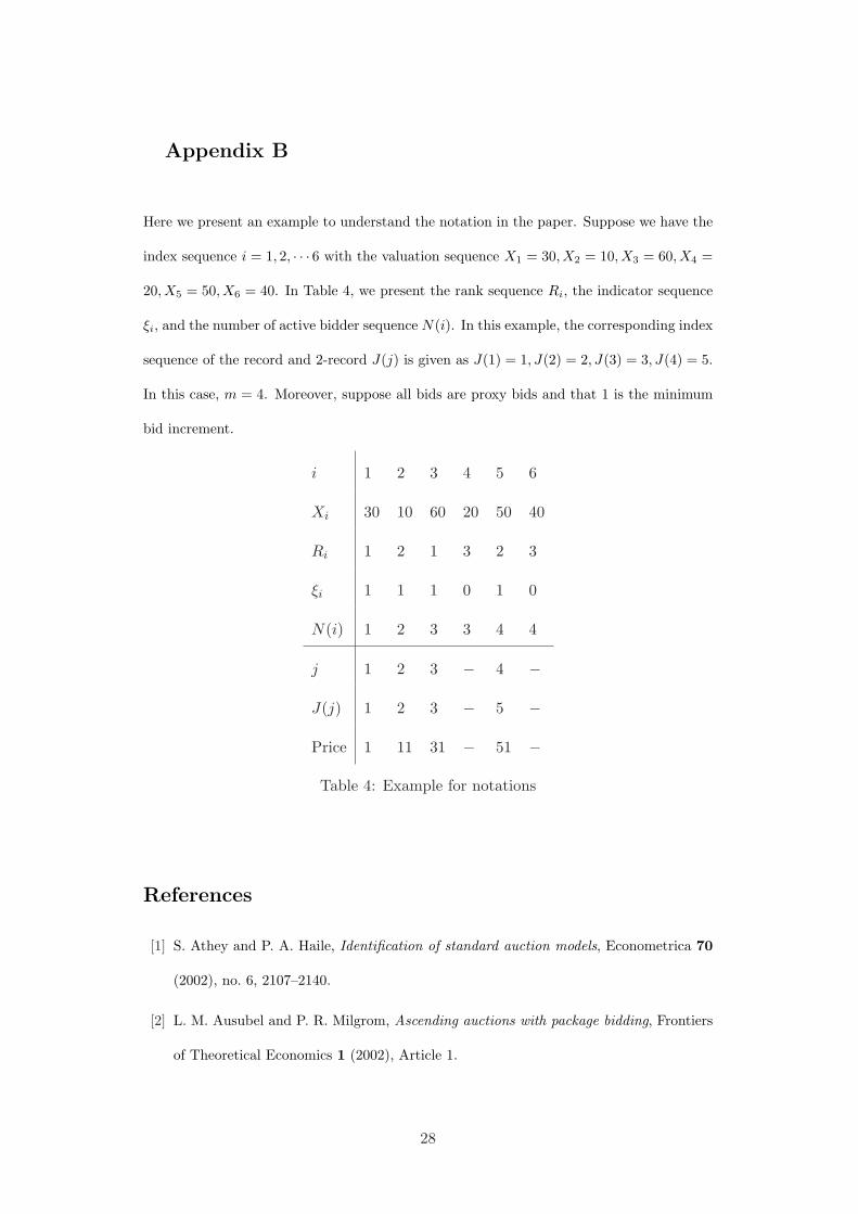
Appendix B
Here we present an example to understand the notation in the paper. Suppose we have the
index sequence i = 1, 2, · · · 6 with the valuation sequence X1 = 30, X2 = 10, X3 = 60, X4 =
20, X5 = 50, X6 = 40. In Table 4, we present the rank sequence Ri, the indicator sequence
ξi, and the number of active bidder sequence N(i). In this example, the corresponding index
sequence of the record and 2-record J(j) is given as J(1) = 1, J(2) = 2, J(3) = 3, J(4) = 5.
In this case, m = 4. Moreover, suppose all bids are proxy bids and that 1 is the minimum
bid increment.
i 1 2 3 4 5 6
Xi 30 10 60 20 50 40
Ri 1 2 1 3 2 3
ξi 1 1 1 0 1 0
N(i) 1 2 3 3 4 4
j 1 2 3 − 4 −
J(j) 1 2 3 − 5 −
Price 1 11 31 − 51 −
Table 4: Example for notations
References
[1] S. Athey and P. A. Haile, Identification of standard auction models, Econometrica 70
(2002), no. 6, 2107–2140.
[2] L. M. Ausubel and P. R. Milgrom, Ascending auctions with package bidding, Frontiers
of Theoretical Economics 1 (2002), Article 1.
28
Page 31
[3] P. Bajari and A. Hortacsu, Winner’s curse reserve prices and endogenous entry: Em-
pirical insights from ebay auction, RAND Journal of Economics 34 (2003), 329–355.
[4] J. I. Bulow and P. D. Klemperer, Auctions vs. negotiations, American Economic Review
86 (1996), 180–194.
[5] S. Caserta and C. G. de Vries, Auctions with numerous bidders, Tinbergen Institute
Discussion Paper 05-031/2 (2005).
[6] R. W. Klein and S. D. Roberts, A time-varying Poisson arrival process generator,
Simulation 43 (1984), 193–195.
[7] V. Krishna, Auction theory, Academic Press, 2002.
[8] J. Laffont, H. Ossard, and Q. Vuong, Econometrics of first price auctions, Econometrica
63 (1995), 953–980.
[9] P. A. W. Lewis and G. S. Shedler, Simulation of nonhomogeneous poisson processes
with log linear rate function, Biometrika 63 (1976), 501–505.
[10] R. P. McAfee and J. McMillan, Auctions with a stochastic number of bidders, Journal
of Economic Theory 43 (1987), 1–19.
[11] A. Ockenfels and A. E. Roth, Late and multiple bidding in second price internet auc-
tions: Theory and evidence concerning different rules for ending an auction, Games
Econ. Behav. 55 (2006), 297–320.
[12] H. J. Paarsch, Deciding between the common and private value paradigms in empirical
models of auctions, Journal of Econometrics 51 (1992), 191–251.
[13] Y. H. Park and E. T. Bradlow, An integrated model for bidding behavior in internet
auctions: Whether, who, when, and how much, Journal of Marketing Research 42
(2005), no. 4, 470–482.
[14] S. I. Resnick, Extreme values, regular variation, and point processes, Springer-Verlag,
1987.
[15] U. Song, Nonparametric estimation of an ebay auction model with an unknown number
of bidders, Working Paper, see http://faculty.arts.ubc.ca/usong/ (2004).
29