Klaus Mosthaf, Mette M. Broholm and Philip J. Binning

DTU , 2014Environment December

The FACT-FLUTe technologyA modeling tool for interpreting field data

1

Contents Preface ........................................................................................................................... 3 

1.  FACT FLUTe ........................................................................................................ 4 

1.1  Technology and installation .................................................................... 4 1.2  Aim .......................................................................................................... 6 1.3  What is measured? .................................................................................. 6 

2.  Model setup ........................................................................................................... 6 

3.  Results: System understanding ............................................................................. 9 

3.1  Behavior of the FACT ............................................................................. 9 3.2  Evolution of the FACT concentration over time ................................... 10 3.3  Hydraulic conductivity .......................................................................... 10 3.4  Flow direction and FACT positioning .................................................. 11 3.5  Initial aquifer concentration .................................................................. 11 3.6  Matrix porosity in the aquifer ................................................................ 12 3.7  Sorption coefficient of the matrix ......................................................... 12 3.8  Porosity of the FACT ............................................................................ 13 

4.  Results: Modeling of Naverland field data ......................................................... 13 

5.  FACT-FLUTe EXCEL data analysis tool ........................................................... 16 

6.  Evaluation and discussion ................................................................................... 16 

Bibliography ............................................................................................................... 17 

2

3

Preface DTU Environment and Region H have established a project to improve knowledge of the fate of contaminants in the limestone aquifers that supply most of the drinking water in Region H. The project aims to improve our understanding of limestone aquifers and develop monitoring methods, improve risk assessment and develop viable alternatives to the commonly employed pump and treat remediation methods. The project involves a combination of field and lab work, and models to interpret the data. This report is an outcome of the modeling part of the project, and addresses the need for new monitoring tools for evaluation of the extent of contamination in chalk aquifers. It is a follow up on the project ‘DNAPL i moræneler og kalk’ where a new FACT-FLUTe monitoring technology was tested in the field. In this follow-on project, the data from the FACT-FLUTe is analyzed using a new modeling tool, which is designed to help interpret FACT-FLUTe data and thereby facilitate the use of the new technology. The following people have participated in the project group: Klaus Mosthaf Mette Broholm Philip Binning We are very grateful for comments we received on the work from Carl Keller, of Flexible Liner Underground Technologies, LLC (FLUTe), USA. The following people from The Capital Region of Denmark have participated in the steering committee for the project: Henriette Kerrn-Jespersen Mads Terkelsen Carsten Bagge Jensen

4

1. FACT FLUTe

1.1 Technology and installation The FACT-FLUTe is a technology which enables the passive monitoring of the contaminant distribution in a monitoring well in fractured limestone aquifers, where a flexible FLUTe liner is placed down the inside of a borehole, as schematically show in Figure 1. There are different kinds of FLUTes, e.g. a water FLUTe (Cherry, Parker, and Keller) and a NAPL FLUTe. The NAPL FLUTe liner has a permeable multi-colored striped membrane (NAPL liner) over the whole length, which can be used to localize the presence of a NAPL. The NAPL dissolves the color on the back of the NAPL liner and leads to a staining where the NAPL phase is located.

Figure 1: Installation procedure for a FLUTe in a borehole.

5

Figure 2: Borehole cross section showing carbon felt absorber (left). FACT as it is inserted in the field, with the NAPL liner and the FACT on the outside (right).

The FACT (FLUTe Activated Carbon Technique) is an activated carbon felt that can be fastened on the outside of the NAPL liner, as shown in Figure 2. When emplaced down the monitoring well, the FLUTe liner is pressurized by adding water, and the FACT is pushed with the liner against the borehole walls. This compresses the 4 cm wide carbon felt from a thickness of 2.5 mm to approximately 0.5 mm. The FACT is protected by an aluminum diffusion barrier on its inside surface. It remains within the borehole for a suitable time period (minimum 1-2 days), where it is able to sorb contaminants from the surrounding aquifer. Afterwards it is removed and cut into segments of, for example, 2 or 10 cm length, which are analyzed for the sorbed contaminant concentrations (mg contaminant per g activated carbon felt), as depicted in Figure 3. This gives a discretized distribution of a contaminant within the vicinity of the borehole and may also help to localize fractures.

Figure 3: FACT with the NAPL liner on the outside (left). Sectioning and sampling of activated carbon felt (right).

6

1.2 Aim The FACT provides very detailed information on the distribution of contaminant next to the borehole, but there is no obvious correspondence between detected concentrations on the FACT and the observed aqueous concentration within the aquifer. This is due to the fact that the aqueous concentrations are usually measured using a minimum 30-50 cm long sampling section in a multilevel/monitoring well, which represents the flow and transport within fractures or higher permeability features of the aquifer, while the FACT measurement is closer to being a point measurement – reflecting the pore water concentrations. Moreover, the emplacement time of the FACT, the hydraulic parameters of the aquifer and the flow and transport processes influence the amount of sorbed contaminant on the FACT. A model can help to determine how the sorbed concentration on the carbon strip is related to the contaminant concentration in the pore water of the aquifer based on the measured aquifer parameters and conditions. This project aimed to set up such a model in order to aid interpretation of the FACT-FLUTe field data. In particular, the project aimed to develop a practical EXCEL data interpretation tool that can be used by practitioners utilizing the technology. The model and tool were tested by examining data collected at the Naverland contaminated site and the data described by Janniche (2013).

1.3 What is measured? The NAPL FLUTe liner can indicate the presence of a NAPL phase, whereas the FACT measures the sorbed contaminant concentration on the activated carbon felt (Sørensen, 2014), which is related to the pore water concentration of the dissolved contaminant at the position of the FACT within an aquifer borehole. Often, the FACT measurements are combined with multilevel water samples, which measure a contaminant concentration in the aquifer. These water samples are likely to be heavily influenced by the presence of fractures, which are often the main flow path for the water. In contrast, the resolution of the FACT is higher and the FACT response is mainly due to diffusion of the contaminant from the surrounding pore water into the carbon felt. The sorbed concentration measured with the FACT can be converted to aqueous concentrations in the pore water with the help of simulations, as shown in this report.

2. Model setup First, the influence of different aquifer parameters on the FACT response is analyzed using a COMSOL Multiphysics® model. Then, a borehole with an installed FACT is simulated based on field measurements in the wells C1-C3 in Naverland. The model simulates the accumulation of a contaminant (PCE) in the FACT during its installation time in a borehole and the contaminant distribution in the limestone aquifer surrounding the borehole. Various modeling geometries have been employed in this study, ranging from simple 1-D models to full 3-D models including both fractures and the limestone matrix. Figure 4 provides an overview of the model domain and the boundary conditions for the 2-D setup (top view). When appropriate, symmetry of the domain was

7

exploited to reduce computational efforts. For the analysis of the influence of the angle between flow and the positioning of the FACT, the entire domain was simulated. To resolve the transport and sorption processes properly, the thin compressed FACT requires a high grid resolution.

Figure 4: Model geometry and boundary conditions. The borehole diameter is 164 mm. Within the borehole is a FLUTe liner all the way around the borehole. At the upstream and downstream ends, between the FLUTe and the NAPL liner at the borehole wall is a FACT strip, here oriented normal to the groundwater flow. The FLUTe liner is not modeled separately.

The set of parameters chosen for the model is listed in Table 1. These parameters are derived from field and lab measurements at the Naverland site. For each parameter, the data source is listed in the table. Single-phase flow with contaminant transport is simulated within the entire domain. Therefore, two equations are solved. The governing equation for stationary flow is given by

∙ ∙ 0, where the water flux q is approximated by Darcy’s law, h is the hydraulic head and K the hydraulic conductivity with different values in the limestone and the FACT. The governing equation for contaminant transport is given by

1 ⋅ ⋅ 0,

with the bulk density , the sorption coefficient , the porosity , the contaminant concentration , and the hydrodynamic dispersion tensor D.

h=1m

h=1m

-I*0

.5m

0.5m

FLUTe

c=30

mg/

L

164 mm

No flow (assumed streamline)

No flow (symmetry)

No flow(symmetry)

Limestone aquifer

Borehole

No flow

FLOW

cinit =30 mg/L

0.25

m

0.25

m

FACT

⋅c

8

Table 1: Overview of chosen parameters for the reference case, which is related to the observations in the boreholes C1 to C3 in Naverland. The FACT parameters are for the compressed case and PCE is considered as contaminant.

Parameter Value Name Source d 16.4 cm borehole diameter Sørensen et al.

(2014) tmax 42 h time FACT was

installed Sørensen et al. (2014)

Dm effective diffusion coefficient

Chambon et al. (2009a)

20.018m /yr free diffusion coefficient of PCE in water

Chambon et al. (2009b)

L 0.1m longitudinal dispersivity

assumed

T 0.01m transversal dispersivity

assumed

FACT Dimensions 0.5 × 40 mm compressed

geometry of cross section

Sørensen et al. (2014)

n 0.84 compressed porosity

deduced from compressed bulk density and crystalline density of carbon (~ 2 g/cm3)

K 10-7 m/s FACT hydraulic conductivity

guess, personal communication with Carl Keller (FLUTe, USA)

dk 12000 L/kg linear sorption coefficient PCE

Sørensen et al. (2014)

b 0.32 g/cm3 compressed bulk density

Sørensen et al. (2014)

Limestone I 1 ‰ hydraulic head

gradient Pedersen and Vilsgaard (2013)

n 0.4 porosity Janniche et al. (2013)

K 10-5 m/s matrix hydraulic conductivity

Janniche et al. (2013)

dk 1.13 L/kg (PCE, w d sc k c )

linear sorption coefficient for PCE in limestone

Salzer (2013)

b 1.75 g/cm3 bulk density Janniche et al. (2013)

9

3. Results: System understanding

3.1 Behavior of the FACT

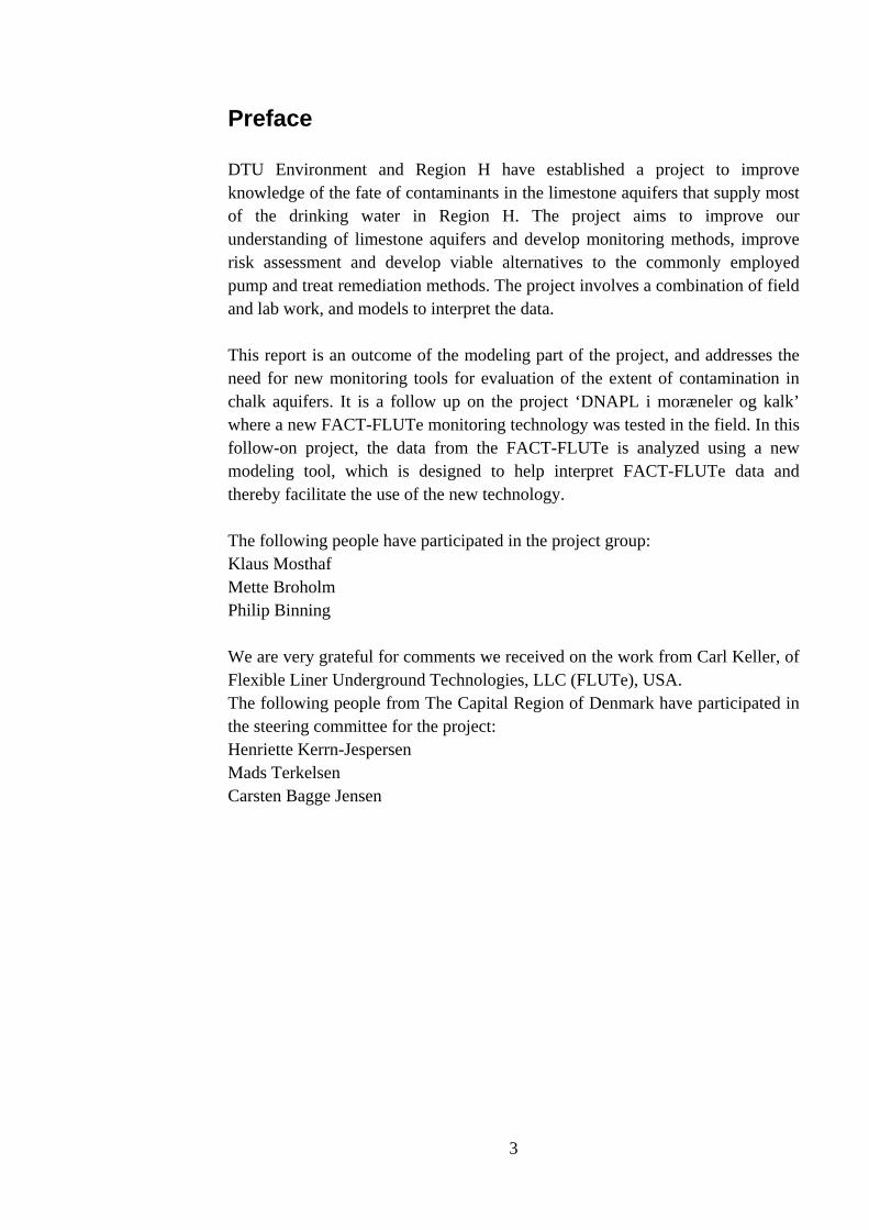
Figure 5: The aqueous PCE concentration distribution in the aquifer and in the FACT after 42 h of exposure to a flow normal to the FACT strips (yellow arrows) is depicted. Here, two FACTs are installed, one in the upstream direction and one in the downstream direction. The figure on the right shows the distribution of sorbed PCE concentration in the compressed FACT after different emplacement times with the contaminant diffusing into the 0.5 mm thick FACT from the right.

Diffusion is the main transport mechanism of contaminant from the region surrounding the borehole into the FACT. The contaminant diffuses from the matrix into the FACT as soon as it is emplaced. This leads to a reduction of the contaminant concentration in the vicinity of the FACT, as can be seen in Figure 5. As a result, the concentration gradient toward the FACT decreases gradually, causing a slowing in time of the mass transfer to the FACT. In contrast, groundwater flow in the formation around the borehole can transport new contaminant towards the FACT, which enhances the concentration gradient and the contaminant flux into the FACT strip. Note that the sorption coefficient in the activated carbon felt is extremely high (Kd of PCE: 12000 L/kg). An example for the spatial distribution of the sorbed concentration within the FACT after different emplacement times is shown in Figure 5 on the right. The contaminant diffuses from the right (x=0.5 mm) into the compressed FACT, leading to a slight decrease of the contaminant concentration in the pore water close to the FACT. The influence of different parameters on the spatially averaged sorbed concentration on the FACT is demonstrated in the following part. Table 2 gives an overview of the tested parameter ranges. Table 2: Overview of tested ranges for the FACT and matrix parameters.

FACT Matrix Unit Flow angle 0-180 degree Cinit 0 0 – 50 mg/L K 10-7 10-8 – 1 m/s n 0.4 – 0.8 0.2 – 0.5 m3/m3 kd 12000 0.01 – 10 L/kg

10

3.2 Evolution of the FACT concentration over time

Time (h)

0 50 100 150 200

Cfa

ct (

mg

/g)

0

2

4

6

8

10

12

14

16

18Caq = 10 mg/lCaq = 30 mg/lCaq = 50 mg/l

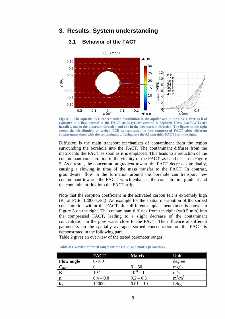
Figure 6: Averaged sorbed FACT concentrations over time for different initial aquifer concentrations and flow normal to the FACT.

The evolution of the sorbed concentration (mg contaminant per g FACT) on the FACT over time for three different initial PCE concentrations within the aquifer and with groundwater flow normal to the FACT is shown in Figure 6. The time where the FACT is in place is important, since the concentration on the FACT continuously increases until equilibrium with the aquifer is attained or the sorption capacity of the FACT is reached. The concentration gradients in the system decrease with time meaning that the rate of accumulation of contaminant in the FACT slows down. In the remainder of this report, a time span of 42 hours will be considered, as this was the emplacement time in the Naverland field experiments.

3.3 Hydraulic conductivity

Hydraulic conductivity (m/s)

10-8 10-7 10-6 10-5 10-4 10-3 10-2 10-1 100

Cfa

ct (

mg/

g)

0

20

40

60

80

100

120normal flowtangential flow

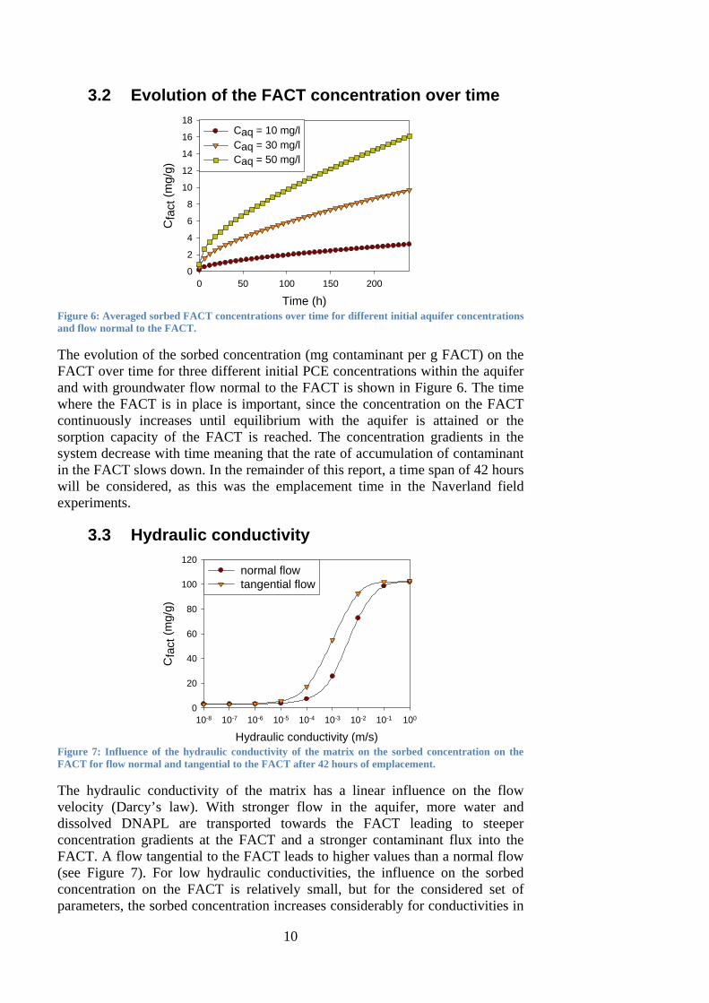
Figure 7: Influence of the hydraulic conductivity of the matrix on the sorbed concentration on the FACT for flow normal and tangential to the FACT after 42 hours of emplacement.

The hydraulic conductivity of the matrix has a linear influence on the flow velocity (Darcy’s law). With stronger flow in the aquifer, more water and dissolved DNAPL are transported towards the FACT leading to steeper concentration gradients at the FACT and a stronger contaminant flux into the FACT. A flow tangential to the FACT leads to higher values than a normal flow (see Figure 7). For low hydraulic conductivities, the influence on the sorbed concentration on the FACT is relatively small, but for the considered set of parameters, the sorbed concentration increases considerably for conductivities in

11

the range between 10-5 and 10-1 m/s. For a hydraulic conductivity higher than 10-1 m/s, the diffusion in the FACT is limited by the transport processes within the carbon felt itself. Hence, the influence of the exterior flow condition becomes less.

3.4 Flow direction and FACT positioning

Angle (degrees)

0 20 40 60 80 100 120 140 160 180

Cfa

ct (

mg/

g)

3,5

4,0

4,5

5,0

5,5

6,0

Figure 8: Sorbed contaminant concentrations on the FACT after 42 hours emplacement time, depending on the angle between groundwater flow and FACT positioning. 0 degrees means flow normal to the FACT.

The angle between groundwater flow and FACT positioning has an influence on the supply of water and contaminant to the formation surrounding the FACT. Figure 8 shows that the highest FACT concentrations occur for flow tangential to the FACT. Here, 0 degrees means flow perpendicular to the FACT, whereas 90 degrees means tangential flow. For parameters typical for the limestone aquifer at Naverland, it can be seen from Figure 8 that the positioning of the FACT relative to the groundwater flow has an impact on the results obtained. However, compared to the influence of the hydraulic conductivity, its influence is relatively small.

3.5 Initial aquifer concentration

Caq (mg/l)

0 20 40 60 80 100

Cfa

ct (

mg/

g)

0

5

10

15

20no flow normal flowtangential flow

Figure 9: FACT concentrations for different aquifer concentrations with different flow conditions: no flow, flow normal to the FACT and flow tangential to the FACT.

Figure 9 shows the effect of the initial aquifer concentration on the sorbed concentration on the FACT. Three different settings are shown, no groundwater flow, flow normal to the FACT strip and flow tangential to the FACT. As can be

12

seen in the figure, flow in the aquifer leads to higher FACT concentrations, with flow tangential to the FACT leading to the highest FACT concentrations. The initial aquifer concentrations and the sorbed concentrations are linearly related, since contaminant transport into the FACT happens primarily due to diffusion. This can be exploited to determine the pore water concentrations from measured FACT concentrations.

3.6 Matrix porosity in the aquifer

Porosity (-)

0,20 0,25 0,30 0,35 0,40 0,45 0,50

Cfa

ct (

mg/

g)

3

4

5

6

7

8

9normal flowtangential flow

Figure 10: Influence of matrix porosity on the FACT concentrations for normal and tangential flow.

Higher aquifer porosity has two counteracting effects: On the one hand it decreases the flow velocity while on the other hand it leads to higher values of the effective diffusivity and increases the amount of contaminant storage in the system. Overall, higher FACT values can be observed for lower porosities (Figure 10). The influence of porosity on the FACT concentrations is pronounced for a strong effect of the flow, as it is the case for tangential flow.

3.7 Sorption coefficient of the matrix

Sorption coeff. Kd (L/kg)

0,01 0,1 1 10

Cfa

ct (

mg/

g)

1

2

3

4

5

6

7

8

9

Figure 11: Influence of the sorption coefficient of the limestone matrix for normal flow.

A higher sorption coefficient in the matrix, e.g. for a different porous material, leads to a higher sorbed concentration on the FACT for the same aqueous concentration in the matrix, because a higher sorption coefficient means that there is more contaminant mass sorbed to the matrix. When the contaminant concentration in the aqueous phase decreases, the sorbed contaminant from the

13

matrix is released. Hence, the concentration gradient towards the FACT remains higher for a longer time, resulting in higher observed values on the FACT (see Figure 11). The measured sorption coefficients for PCE in the considered limestone are 1.1 L/kg, for TCE 0.4 L/kg and for cis-DCE 0.2 L/kg (Salzer, 2013).

3.8 Porosity of the FACT

FACT porosity (-)

0,4 0,5 0,6 0,7 0,8 0,9

Cfa

ct (

mg/

g)

1,5

2,0

2,5

3,0

3,5

4,0

4,5

Figure 12: Influence of the FACT porosity on the sorbed concentration on the FACT. The porosity of the FACT may change due to compression.

The FACT is compressed during installation, leading to a change in bulk density, porosity and permeability. Figure 12 shows the influence of the porosity of the FACT on the computed FACT concentrations. Since the effective diffusion coefficient in the FACT is related to the relative pore space expressed by the porosity, higher FACT porosities lead to higher FACT concentrations. In this report, a FACT porosity of 0.84 is employed for the compressed FACT, which is deduced from the bulk density of the FACT and the crystalline density of activated carbon of 2 g/cm3.

4. Results: Modeling of Naverland field data The model was employed to analyze field data measured at the boreholes C1-C3 at Naverland. The procedure was to determine the relation between initial aqueous concentration and sorbed FACT concentration with the model for a given set of parameters and to use this relation to convert measured FACT concentrations from the boreholes to pore water concentration in the limestone matrix. In each case, the model parameters were fixed as shown in Table 1. The hydraulic conductivity was selected as the maximum and minimum observed conductivity values in the borehole. Results are depicted in Figure 13, with the left panel showing water samples which were taken at Naverland (borehole C1 – C3) at different depths from Water FLUTe multilevels with sample lengths of 30-50 cm. The multilevels were installed in the same borehole, where the FACT had been exposed to the contaminated aquifer for 42 hours approximately half a year earlier. The conditions in the aquifer are assumed to have remained constant within this time

14

period. A remedial pumping system operated continuously at the site, was turned off after sampling of the multilevels in April. When the water potentials were stable, the multilevels were sampled again (May sampling round) before the pump was turned back on. The graphs on the left in Figure 13 show the aqueous concentrations measured in the water samples from the two sampling rounds (April and May). The differences in the curves between April and May (especially in C2 and C3) illustrate the effect of the remedial pumping and of back-diffusion of the contaminant from the matrix into higher permeability zones, after the remediation well was turned off. The sorbed concentrations measured on the FACT located within these intervals were selected and converted from FACT concentrations (mg/g) to pore water concentrations in mg/l using the simulation of two different values for the hydraulic conductivity in the aquifer, the minimum and maximum value observed in the borehole. Since the equations are linear, once all the model parameters have been fixed, it is possible to obtain a simple conversion factor which is the ratio of the FACT concentration to that in the limestone matrix at the time of emplacement of the FACT. These conversion factors and the respective hydraulic conductivities are listed in Table 3. The converted concentrations from the FACT measurements at Naverland are shown in the right graph of Figure 13. The individual FACT values were averaged according to the length of the water samplers to obtain the average concentration values at these depths. As can be seen, there is a good correspondence between the modeled porewater concentrations and the measured concentrations in groundwater samples from multilevels in terms of the concentration distribution. The magnitude of the concentrations is nearly comparable for the maximum conductivity case, whereas the porewater concentrations based on FACT analysis for the low conductivity, or diffusion controlled, case are significantly higher than concentrations of samples from the multilevels. This is consistent with the expectation, that the water samples from the multilevels predominantly represent the most conductive fractures, and with the observation of concentration rebound after the remedial pumping was turned off, caused by matrix back diffusion. Table 3: Conversion factors deduced from the simulations of the highest and lowest observed conductivities for the three boreholes at Naverland.

C1 C2 C3 Kmin 7×10-7 m/s 3.5×10-7 m/s 10-6 m/s Kmax 2×10-4 m/s 10-3 m/s 5×10-4 m/s Cpore/Cfact (Kmin)

9.47 9.54 9.41

Cpore/Cfact (Kmax)

2.9 1.17 1.74

15

Cw (mg/l)

0 50 100 150 200 250

Dep

th (

m)

8

10

12

14

16

18

AprilMay

Cw (mg/l)

0 50 100 150 200 250

8

10

12

14

16

18

K=2e-4 m/sK=2e-4 m/s (average)K=7e-7 m/s (average)

Aq. concentrations from water samples (C1) Aq. concentrations computed from FACTs

Aq. concentrations from water samples (C2)

Caq (mg/l)

0 20 40 60 80

Dep

th (

m)

8

10

12

14

16

18

20

AprilMay

Aq. concentrations computed from FACTs

Caq (mg/l)

0 20 40 60 80

8

10

12

14

16

18

20

K=1e-3 m/sK=1e-3 m/s (average)K=3.5e-7 m/s (average)

Aq. concentrations from water samples (C3)

Caq (mg/l)

0 20 40 60 80

Dep

th (

m)

8

10

12

14

16

18

20

AprilMay

Aq. concentrations computed from FACTs

Caq (mg/l)

0 20 40 60 80

8

10

12

14

16

18

20

K=1e-6 m/sK=1e-6 m/s (average)K=5e-4 m/s (average)

Figure 13: Aqueous concentrations measured with water samples at different intervals from multilevel samples with a length between 30 and 50 cm (left), and FACT values converted to pore water concentrations using the relation between the FACT and pore water concentration obtained from the numerical simulations (right). In the right hand panel, the points show the direct conversion of FACT measurements to aqueous concentrations (pore water), and the lines show the average concentrations for intervals corresponding to multilevel screen length. Hence, the lines in the right hand panel may be compared with the lines in the left hand panel. Note, however, that the water samples will draw more water from the fractures than from the matrix due to preferential flow in the fractures, whereas the model results assume only diffusive transport. The minimum and maximum hydraulic conductivity observed in each borehole was simulated to obtain the two different distributions in the right panel.

16

In the latter case some of the FACT based porewater concentrations in C1 for the low conductivity/diffusion controlled case are higher than the effective solubility of PCE in water in the mixed PCE and TCE contamination. This is naturally not possible, and hence an indication of the presence of DNAPL. However, it may also be caused by matrix flow. For borehole C1, the potential presence of DNAPL is also consistent with the continuously high aqueous concentrations in multilevel samples (with and without pumping).

5. FACT-FLUTe EXCEL data analysis tool A simple EXCEL spreadsheet tool has been developed to convert FACT data into equivalent matrix pore water concentrations. In the tool, the user can set the aquifer and FACT parameters and sampling time, and then the appropriate conversion factors (see Table 3 for those calculated for Naverland) are returned. The spreadsheet is designed to show plots of the relevant field data and inferred model results. The user can then vary parameters and immediately see how they influence the data conversion.

6. Evaluation and discussion The simulation results show that a multitude of parameters influences the observed sorbed concentrations on the FACT. The hydraulic conductivity has the strongest effect (up to orders of magnitude), whereas the effect of the matrix porosity and the angle between groundwater flow and FACT positioning was comparatively small. If the hydraulic parameters and conditions in the aquifer are known, the prevailing pore water concentrations can be obtained from the FACT measurements with the help of the linear relationship between FACT concentrations and pore water concentrations. The qualitative distribution remains the same for different parameter sets, but the magnitude of the curve changes. The ratio between observed FACT concentrations and pore water concentrations can be determined with the help of a numerical model. The differences between the concentrations determined with the water samples and with the FACTs can be partly attributed to the assumption of a homogeneous parameter distribution within the borehole. Moreover, they are likely to be due to the influence of the water flow within fractures or high-conductivity zones, which strongly influences the measured concentrations in the water samples. The remedial pumping may have changed the groundwater flow direction and transported water from further away to the wells through these high-conductivity features. To obtain a good representation of the aquifer concentrations at different locations, the variability of the aquifer parameters can be taken into account. The FACT provides a much higher spatial resolution of monitoring data than water samples and potentially allows for fractures that contain a DNAPL phase to be located within the borehole. Hence, the FACT is a helpful tool to obtain a detailed contaminant distribution within an aquifer.

17

Bibliography Chambon, Julie, Ida Damgaard, Camilla Christiansen, Gitte Lemming, Mette M.

Broholm, Philip J. Binning, and Poul L. Bjerg. “Model assessment of reductive dechlorination as a remediation technology for contaminant sources in fractured clay. Modeling tool, Delrapport II.” DTU Environment, Environmental Project No. 1295, 2009, Miljøproject, 2009a.

Chambon, Julie, Gitte Lemming, Mette M. Broholm, Philip J. Binning, and Poul L. Bjerg. “Model assessment of reductive dechlorination as a remediation technology for contaminant sources in fractured clay. Case studies, Delrapport III.” DTU Environment. Environmental Project No. 1296 2009, Miljøproject, 2009b.

Cherry, John A., Beth L. Parker, and Carl Keller. “A New Depth-Discrete Multilevel Monitoring Approach for Fractured Rock.” Ground Water Monitoring & Remediation 27.2 (2007): 57–70.

Janniche, Gry S., Annika S. Fjordbøge, and Mette M. Broholm. “DNAPL i moræneler og kalk – vurdering af undersøgelsesmetoder og konceptuel modeludvikling.” DTU Environment, 2013.

Pedersen, Lise C., and Kristine D. Vilsgaard. “Evaluering af afværgepumpning til afskæring af en forurening medklorerede opløsningsmidler i et kalkmagasin.” DTU Environment, 2013.

Salzer, Joel P. “Sorption capacity and governing parameters for chlorinated solvents in chalk aquifers.” Master thesis, DTU Environment, 2013. Sørensen, Mie B. and Mette M. Broholm. “Sorption af chlorerede opløsningsmidler på FACT.” DTU Environment, 2014.