The Faculty of Engineering and Science Department of Computer Science TITLE: Improving quality of keyword query results using ESKuSE PROJECT PERIOD: DAT6, 01-01-2003 - 06-06-2003 AUTHOR: Martin Christensen PROJECT SUPERVISOR: Heidi Gregersen NUMBER OF COPIES: 5 TOTAL PAGE NUMBERS: 33 This report presents the ESKuSE keyword search engine: a fast and efficient key- word search engine that searches relational databases. It models database schema as graphs and uses graphs extensively in its ex- ecution of queries. Based on hints provided at different levels in the database, it makes informed guesses about the data on a conceptual level rather than just a logical. Martin Christensen
Transcript
The Faculty of Engineering and ScienceDepartment of Computer Science
TITLE:Improving quality of keyword query resultsusing ESKuSE
PROJECT PERIOD:DAT6,01-01-2003 - 06-06-2003
AUTHOR:Martin Christensen
PROJECT SUPERVISOR:Heidi Gregersen
NUMBER OF COPIES: 5
TOTAL PAGE NUMBERS: 33
This report presents the ESKuSE keywordsearch engine: a fast and efficient key-word search engine that searches relationaldatabases. It models database schema asgraphs and uses graphs extensively in its ex-ecution of queries.Based on hints provided at different levels inthe database, it makes informed guesses aboutthe data on a conceptual level rather than justa logical.
This report is a continuation of the work presented in [4], although the present report can be readindependently of its predecessor. It describes ESKuSE, an acronym forESKuSE is aStructurelessKeyword query Search Engine, which is a fast and efficient keyword search engine for relationaldatabases.
1.1 Motivation
Today, large amounts of data are stored in relational databases. They are almost exclusively queriedin a structured fashion using query languages such as SQL. A user who wishes to issue his ownqueries on the database must have knowledge of its schema, and must either use SQL (or equivalentlanguages) or rely on e.g. graphical query design tools. Most users, however, only interface indirectlywith the database through applications that hide communication with the database through predefinedqueries.
This imposes several restrictions on the user. First of all,it raises the bar on the qualificationsneeded to issue queries. Secondly, structured queries willonly return the results that the user expectsto get, whereas keyword queries might also find results that are unexpected. Thirdly, structured queriesallow almost no vagueness, but the user may not have enough information to make an adequatelyprecise query.
Keyword querying will not displace structured querying in its current roles, since the latter hassignificant benefits with regard to control of the query results and raw performance, but the two com-plement each other well. Perhaps most significantly, keyword query engines can dramatically reducethe effort required to publish structured data and subsequently perform queries on these data [2].
The great success Internet search engines shows that peoplewith no special training or educationtake very easily to using keyword queries to find relevant information on the Internet. Keyword searchengines for relational databases can present users with a similar interface, which will thus be bothfamiliar and unintimidating to even inexpert users. This could easily prove to become a significantnew source of information on corporate networks, though thegeneral method is still very young, andhas not yet seen widespread usage.
1.2 Keyword queries
Today, we know keyword queries primarily from Internet search engines. We can enter our query as alist of keywords, which are normally just words and/or numbers, and that’s all the search engine needs
2
to find documents that match our query. While a relational database is very different from a collectionof web pages, queries may well look exactly the same and be expected to return results in much thesame way.
Keyword queries, by their nature, offer only limited expressive power. As we know them fromInternet search engines, keyword queries are normally either considered conjunctive or disjunctive.Consider a keyword query as a set of keywordsfa; b; g. A conjunctive query will require all keywordsto be found, i.e.a ^ b ^ , and a disjunctive query will require at least one keyword tobe found, i.e.a _ b _ .
Most search engines, though, allow a combination of the two,which is to say that some keywordsare specified to be required, typically by prefixing the keyword with a +, and the remainder areoptional. Given such rules, the queryf+a; b; g would be expressed asa_(a ^ (b _ )). Furthermore,exclusion of certain keywords, commonly denoted by prefixing the excluded keyword with a�, is alsosupported by most search engines, wheref�a; b; g would be expressed:a ^ (b _ ). The+ and�prefixes add significant improvements in expressive power ofa query while not adding significantlyto the complexity of the query itself. Generally, exclusive-or queries are not supported.
The popularity of today’s Internet search engines shows that people generally are comfortablewith using keyword queries. When submitting a keyword queryto a search engine, the usual wayof thinking of it is as being ‘as conjunctive as possible’, i.e. the user expects as many keywords aspossible to be found, but if not all of them can be found in any one result, fewer will suffice. Let’scall these queries ‘mostly conjunctive’ as opposed to ‘strictly conjunctive’, the latter which will be atrue conjunctive query. The impreciseness in this form of query can either be hidden in more complexlogical expressions of the query than is shown here, or, perhaps more likely, in some ranking system.In the latter case, the query might be entirely disjunctive,but the ranking system could favour resultsin which many of the keywords in the query occur. Fortunately, all this complexity is hidden from theview of the user, who can usually get good search results without any knowledge of the underlyingsystem.
1.3 Related work
The work presented in this report is the continuation of [4].The ESKuSE system has seen considerablespeed improvements since the writing of aforementioned report, and the quality of search results hasbeen significantly increased. Speed improvements have beenintroduced mainly through simple mass-query optimisation, which dramatically reduces the numberof SQL queries necessary to perform foreach keyword query, especially on more complex queries. Furthermore, an algorithm that generates‘templates’ for all possible candidate networks, which arethen stored in the schema graph, therebyavoiding many redundant calculations. Quality improvements are achieved by improving the algo-rithms involved in executing the query, by making informed guesses about the conceptual databasemodel based on information about the logical database model, and by adding to the expressive powerof keyword queries.
ESKuSE is in many ways similar to the DISCOVER system presented in [7]. DISCOVER’smethod of ranking query results is implicit in its search algorithm. ESKuSE allows for differentranking techniques, but currently it only uses graph weights in its data structures for this purpose.DISCOVER, using its Master Index, is able to locate precisely the tuples containing keywords, butonly uses this knowledge to generate tuple sets, where it could possibly also be used to further optimiseSQL queries. DISCOVER has a practical upper limit of candidate network sizes of around5� 6 on a100 MB database; larger candidate networks take a prohibitively long time to evaluate. This limits the
3
usefulness of the system to either small queries or small databases. For queries to take prohibitivelylong for ESKuSE to perform on a database of similar size, either the query must consist of very manykeywords, or one or more of the keywords in the query must appear in thousands of tuples. The formerproblem should be considered a user error, and the latter problem will often be solved by removing‘too common’ words from the index like Internet search engines most often do.
In the BANKS system, described in [2], a database is perceived as a graph in which every tuple is anode, and where relationships represent edges. Since the entire database is perceived as a graph, whichis held in main memory, this graph will be larger than the database itself, setting a much lower limitto the size of database that can be practically searched thanESKuSE. ESKuSE’s query graphs andcandidate networks can be considered incomplete or uninstantiated subgraphs of the larger graph thatBANKS uses. The authors employ a ranking system similar to that of Google [3], where referencesto tuples count as votes. Also they use the ‘fan out’ of connecting nodes in ranking: if a query isperformed on the relationship between two people, and they both belong to a group of 6 people andanother group of 100 people, then the smaller group will be taken to be the closer relationship. Thisranking technique has been adapted for use in ESKuSE. BANKS provides a means for the user tointeractively refine query results. Currently, ESKuSE onlyreturns final, unalterable results, but it ispossible that ESKuSE could be made to support something similar with fairly minor changes to theexisting code base.
DBXplorer’s symbol tables, described in [1], are much like the index used in ESKuSE. The pa-per explores different indexing strategies which could prove valuable to further work on ESKuSE’sindex, but which would require completely rethinking keyword nodes. A problematic limitation ofDBXplorer is that it cannot connect two tuples in the same relation.
1.4 Problem definition
This project aims to finish the work started in [4] and create afully functional keyword search enginebackend for relational databases that is practically usable in production environments.
To meet this goal, two equally important subgoals must be met:� query results must be returned quickly, and� query results must be of high quality.
Being intended for interactive use rather than batch processing, ESKuSE should be able to returnresults to most queries within a matter of seconds, or the point of interactive use is soon lost. Thus thespeed issue becomes important. The importance of high-quality query results is obvious, since no-onewill want to use a search engine that yields mostly useless results.
1.5 Composition of the report
This report is laid out as follows.Chapter 2 presents the basic ESKuSE system. It provides a walk-through of the ESKuSE ar-
chitecture, defines the data structures used and describe the main algorithms involved in performingkeyword queries. Also, it describes the most important speed optimisations.
Chapter 3 discusses the concept of quality in query results,and it presents the techniques thatESKuSE uses to improve its results.
Chapter 4 presents and discusses the tests that have been performed with ESKuSE and their results.
4
Chapter 5 concludes the report and discusses possible future work.
5
Chapter 2
ESKuSE fundamentals
This chapter describes the basic ESKuSE system. It is meant to address some of the clarity issuesin [4]. Many of the unused implementation options mentionedin [4] are omitted from this paper so asto not add unnecessary complexity.
ESKuSE is a search engine that searches arbitrary relational databases. The basic units that wesearch for with ESKuSE are keywords. To formalise the notionfrom Chapter 1.2, the followingdefinition is given:
Definition 2.1 (keyword) A keywordkw is a tuple(TY PE; value), whereTY PE is the data typeof the keyword, andvalue is the what is being searched for in the database. Thevalue element mustbe of typeTY PE.
From this, the definition of keyword queries follows trivially:
Definition 2.2 (keyword query) A keyword queryQ is a set of keywordsfkw0; kw1; : : : ; kwng.As an example,(STRING; john) and(INTEGER; 42) are possible keywords, and they can formthe keyword queryf(STRING; john) ; (INTEGER; 42)g.
With a proper definition of keyword queries in hand, we can begin to explore how they are pro-cessed.
2.1 Architecture
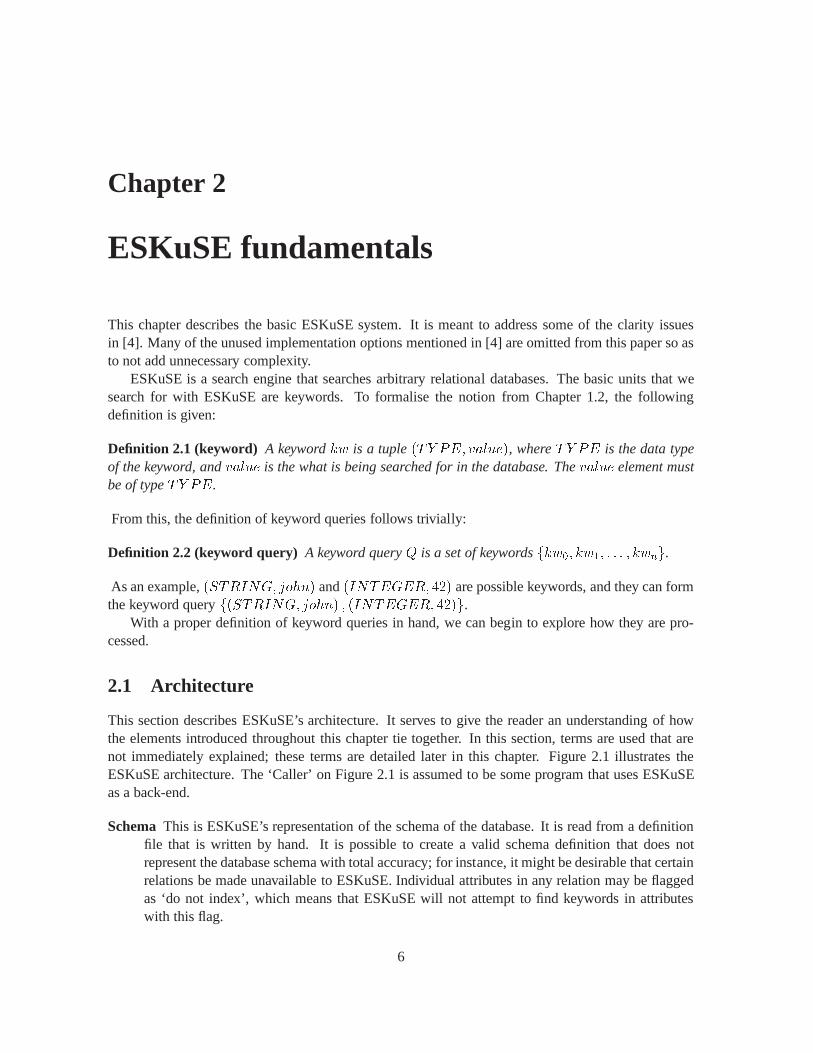
This section describes ESKuSE’s architecture. It serves togive the reader an understanding of howthe elements introduced throughout this chapter tie together. In this section, terms are used that arenot immediately explained; these terms are detailed later in this chapter. Figure 2.1 illustrates theESKuSE architecture. The ‘Caller’ on Figure 2.1 is assumed to be some program that uses ESKuSEas a back-end.
Schema This is ESKuSE’s representation of the schema of the database. It is read from a definitionfile that is written by hand. It is possible to create a valid schema definition that does notrepresent the database schema with total accuracy; for instance, it might be desirable that certainrelations be made unavailable to ESKuSE. Individual attributes in any relation may be flaggedas ‘do not index’, which means that ESKuSE will not attempt tofind keywords in attributeswith this flag.
6
Index
DB
Schema
Schema graph
Query grapher
CNG
CN evaluator
JNT postprocessor
Index look−up
Joining networks of tuples
Query: (STRING, john), (INTEGER, 42)
Query graph
Candidate networks
Joining networks of tuples
Caller
Caller
Stored data Process
Tuples IDs: (id0, (STRING, johnson)), ...
Figure 2.1: Model of ESKuSE’s architecture. The rounded boxes to the left represent data resources,and the sharp-edged boxes to the right represent processes.Solid lines with arrows represent dataflow, and punctured lines represent dependency on data resources.
Schema graph The schema graph is a graph representation of the logical database structure as de-scribed by the above mentioned schema description.
Index This is a database-wide index that it used to find the tuples that given keywords can be foundin. It is basically an inverted file index. When given a keyword as an input, it returns iden-tifiers all indexed tuples that the keyword can be found in. A tuple identifier has the form(relation; pkvalue), whererelation is the relation that the tuple belongs to, andpkvalue isthe value of the primary key of the tuple. For this reason, only relations with primary keys maybe indexed.
Index look-up This component looks up the keywords it receives from the calling program and out-put the tuple identifiers for the tuples that each keyword wasfound in.
Query grapher Based on the stored schema graph and the tuple identifiers from above, the thiscomponent creates a query graph for the current keyword query.
CNG The CNG (candidate network generator) finds candidate networks in the query graph it receivesas input, eliminates any redundancy in the candidate networks and outputs them.
CN evaluator This component translates the candidate networks it receives into SQL queries, whichit then executes. This yields joining networks of tuples, which it outputs. The translationfrom candidate network to SQL query requires knowledge of primary keys and foreign keyrelationships, which is obtained from ESKuSE’s internal schema representation.
JNT postprocessor The joining networks of tuples received from the previous component are com-bined as described in Chapter 2.3 and output according to rank, best ranking results first.
7
2.2 Data model
Schema structure information is presented on a well-known form by representing the schema as agraph.
First, let’s examine our database schema. LetS = (R;K) be the schema over our database ofinterest, whereR = fr0; r1; : : : ; rng is the set of relations inS, andK = fk0; k1; : : : ; kmg is the setof foreign key relationships between relations inS. Eachki 2 K is represented as(rk; rl), rk andrlbeing relations inR, where there’s an attribute inrk that is a foreign key referencing an attribute inrl.It may be allowed thatk = l.
Using the above, we can define our graph to represent the schema. We call such graphs schemagraphs. They are directed, weighted graphs and contain onlyone node type: relation notes.
Definition 2.3 (relation node) A relation noden corresponds to exactly one relationr 2 R, whereR is the set of relations in our schema.
As a matter of terminology,n is said to representr, or, conversely,r maps ton. The notationr ! n is used to show thatr maps ton.A basic schema graph directly represents a schema without trying to make implicit information
explicit. This type of graph is what was called a naı̈ve schema graph in [4]. It serves as the basis forcreating more elaborate schema graph as we’ll see in Chapter3.
Definition 2.4 (basic schema graph)LetGS = �NS ; ES� be the basic schema graph forS, whereNS is the set of relation nodes in the graph, andES is the set of edges.NS = fn0; n1; : : : ; nngwhere each element inR is represented by an element inNS.
Each edgee 2 ES is represented as(nk; nl; w), wherenk; nl 2 NS, andw is the weight of theedge.ES is defined as8 (rk; rl) 2 K 9nk; nl (rk ! nk ^ rl ! nl)) (nk; nl; 1) ; (nl; nk; 2) 2 ES .
As an example of a basic schema graph, consider the simple schema(fr0; r1g; f(r0; r1)g). Ifr0 ! n0 and r1 ! n1, this schema will be represented by the basic schema graph depicted inFigure 2.2(a).
Schema graphs are not used directly in queries. We assume that the database schema only veryrarely changes, and thus the schema graph that represents itneed only change equally rarely. If theschema changes, the schema graph must be rebuilt.
When a query is performed, a query graph is built based on the schema graph. This schema graph canbe a basic schema graph or a more advanced schema graph, but the procedure for building the querygraph will be the same. A query graph is built from the schema graph, i.e. the schema graph will be asubset of the query graph.
The main thing that distinguishes a query graph from a schemagraph is the presence of anothernode class: keyword nodes.
Definition 2.5 (keyword node) A keyword noden0 represents a tuplet 2 r, wherer 2 R. LetQbe a keyword query. There exists a non-empty set of keywordsKW t = fkw0; kw1; : : : ; kwng, whereKW t � Q, such that eachkwi 2 KW t can be found at least once int, and nokwj can be found int such thatkwj 2 Q ^ kwj 62 KW t.
8
As a matter of notation, a keyword noden0 is said to represent both the tuplet, the set of keywordsKW t and every element ofKW t. Furthermore, ift 2 r, thenn0 is said to stem from the relationnoden, wherer ! n.
When we perform a keyword query, keyword nodes represent thelocations of the data we areinterested in. When we insert keyword nodes into the query graph in the appropriate places, we willhave sufficient information to create SQL queries to determine if and how the tuples that the keywordnodes represent are connected.
Definition 2.6 (query graph) Let query graphG0S be created for a queryQ = fkw0; kw1; : : : ; kwngover schema graphGS . For every tuple in the database that contains at least one keyword, a keywordnoden0 is created to represent it. Ifn0 stems fromn, thenn0 will be given the same edges with thesame weights leading to and from it asn.
For an example of a simple query graph, consider the example basic schema graph given above. Ifsome keyword is found in some tuple in the relation that maps ton1, the resulting query graph will bethe one depicted in Figure 2.2(b).
n0 n112(a) Schema graph
n0 n1n011 212(b) Query graph.n01 is a keywordnode
Figure 2.2: Simple examples of a basic schema graph and a query graph built from it.
The two classes of graphs that have just been described are used to represent the data that queriesare performed upon. Using these, we can adequately describea keyword query. However, they areinsufficient to describe the results yielded by such queries.
Consider the following facts:� schema graphs, and by extension query graphs, accurately represent the underlying logicalstructure of the database,� the information we are after can be found in the result set of some SQL query,� SQL queries are expressed through a combination of keyword information and structural infor-mation, both of which are present in the query graph.
Given these facts, we now know that it is possible to represent the eventual result of a keywordquery as a subgraph of the query graph, because it can be transformed into an SQL query whose resultset is relevant to the keyword query. Because of the limited expressive power of keyword queries as
9
discussed in Chapter 1.2, it is not necessary to use more complicated SQL queries than can adequatelybe expressed by ESKuSE’s data structures.
The result of a keyword query is the result set of one or more SQL join queries, just as it quiteoften is when we use SQL directly. These results will be joining networks of tuples, which are, asthe name implies, tuples that join, i.e. the result of a joining SQL query. When working with querygraphs, we can’t tell which tuples join and which do not, justas we can’t tell what the result set ofan SQL query will be (most of the time). When writing SQL queries, we specify what we want ourresult set to look like and how we want to narrow it. It is exactly the same thing we do when workingwith query graphs. To represent the possible joining networks of tuples on the graph level, we havecandidate networks. We might say that candidate networks are templates for our query results.
In [7], the authors describe two properties of their JoiningNetworks of Tuple Sets, namely thatthey can betotal andminimal. These properties are also useful for ESKuSE, and they are given thefollowing meanings:
Let a query graphG0S be created over schema graphGS based on queryQ. Consider a subgraphT of G0S that is a tree.T is total if all keywords inQ are represented by at least one keyword node inT , andT is minimalwhen the root node and every leaf node is a keyword node.With these definitions in hand, the definition of candidate networks follows simply:
Definition 2.7 (candidate network (CN)) Let T be a subgraph of query graphG0S . If T is a treeand it is minimal,T is a candidate network (CN).
With CNs being minimal, we help prevent superfluous data from‘polluting’ the results. UnlikeDISCOVER, ESKuSE does not require CNs to also be total, meaning that keyword queries are notstrictly conjunctive.
So far, we have only dealt with data descriptions and pointers to data. As mentioned previously,CNs can be translated into SQL queries. This makes bridging the gap between data descriptions andconcrete data, as represented by joining networks of tuples, easy.
Definition 2.8 (joining network of tuples (JNT)) A joining network of tuples (JNT) is an instantia-tion of a CN.
A set of JNTs is the final result of a query.This concludes the definition of all ESKuSE’s central data structures, from the input received from
the caller to the final output that it will be given in return.
2.3 Basic algorithms
This section describes the algorithms used in the current CNG and JNT postprocessor.First, please note that there is a restriction on how the CNG that ESKuSE currently uses generates
CNs, which is simpler than the definition of CNs given. Currently, CNs do not branch (DISCOVERcalls non-branching CNssequences), and they only contain two keyword nodes, one at either end.Assuch, the JNTs that the CNs generate can be thought of as pairsof relevant and related tuples.
The ‘relatedness’ of data is defined by the important constant MaxPathLen, whose role willpresently be described. As we already know, CNs are created from query graphs, and query graphsare weighted, directed graphs. Consider a CN as a path through the query graph. The length of thepath will be the sum of weight of the edges in the CN in the direction from the root to the leaf. If thelength of the path is greater thanMaxPathLen, then the tuples at either end are not considered to
10
be related, and thus the path is not accepted as a CN, since theuser will not want the search results tocontain unrelated data.MaxPathLen should be set with some care: if it has too small a value, theCNG will ignore data that should be considered related, and if it has too large a value, data may beincluded that should not be considered related.
Consider the following example. If two tuples join without any intermediate tuples (e.g.SELECT* FROM r1, r2 WHERE r1.pk = r2.fk), there is obviously bound to be a close relationshipbetween the two tuples, but if there are many intermediate tuples (e.g.SELECT * FROM r1, r2,..., rn WHERE r1.pk = r2.fk AND ...AND r(n-1).pk = rn.fk), the data in thetuples at either extreme are not likely to be closely related.MaxPathLen also impacts performance. Since it indirectly affects the largest allowed size ofCNs, it also affects the size of the largest SQL join queries that the DBMS must perform.
Now thatMaxPathLen has been accounted for, we can look at how the two components work.Initially, the CNG receives a query graph. Algorithm 2.1 shows the Python code use in the pre-
vious implementation of the CNG algorithm. Due to optimisations described in Chapter 2.5, thesecomputations have been moved elsewhere, but the algorithm shows how the CNG works conceptu-ally. It employs a depth first search-like algorithm to search from each keyword node in the querygraph. Whenever another keyword node is reached from the start node that does not make the sumof the weight of all the edges between the start node and the current node larger thanMaxPathLen,the subgraph on the current path is appended to the list of CNs.
When all possible CNs from each node have been calculated, redundancies will be found andeliminated. Consider two CNsa; b; and ; b; a. They represent the same information, and thus theyare redundant. Whichever of them has the larger sum of edge weights is removed, or if they have thesame weight, one is chosen arbitrarily for removal.
The now redundancy-free list is output from the CNG and passed to the CN evaluator, whichcreates JNTs from the CNs. The evaluation process itself is very straightforward: an example of itsuse is given in Chapter 2.4, and more information can be foundin Chapter 2.5. The list of JNTs ispassed to the JNT postprocessor.
First, here’s a short overview of how the JNT postprocessor works conceptually: It creates com-posite JNTs from the smaller JNTs it receives. It does this byfirst creating an undirected graph fromthe received JNTs: its nodes represent the same tuples that were represented by keyword nodes in thequery graph, and its edges are the JNTs that join the different tuples. The resulting graph may notbe connected. The composite JNTs will each span an entire connected component within the graph.Because of the way that the ESKuSE implementation handles JNTs internally, it would be impracticalto use actual code snippets to illustrate the algorithms like above, so instead pseudo-code algorithmsare given, though using Python syntax.
The algorithm for creating the JNT graph is given in Algorithm 2.2. Conceptually, this graphcan be considered an instantiation of a query graph. Consider a basic JNTt0; t1; : : : ; tn as outputby the CN evaluator, where1 � n � MaxPathLen. We know thatt0 andtn are tuples that wererepresented by keyword nodes, or the network that the JNT wascreated from would not be minimaland thus not a CN. We also know thatt0 and tn may be shared with other JNTs because the samekeyword nodes may appear in several CNs. It then makes sense to think of t0 andtn as nodes in agraph, andt1; : : : ; tn�1 as an undirected edge connecting them. This is how JNT graphsare created.
Consider the JNTt0; t1; : : : ; tn from before and another JNTtn; tn+1; : : : ; tn+m. Because theyhave the tupletn in common,t0; t1; : : : ; tn+m will also be a JNT. In this way, we can continue mergingJNTs that share tuples into composite JNTs. This is the principle behind Algorithm 2.3. It starts with
11
MPL = 3 # Constant MaxPathLen. It may be different from 3.
def crawl(g, s): # Takes a query graph and a start node. Initialise the crawl.
Algorithm 2.1: CNG algorithm used to find paths of sizeMaxPathLen or less.
def mk jntgraph(keywordnodes, jnts): # Takes a list of all keyword nodes from the query# graph and all JNTs from the CN evaluator.
jntgraph = graph()
5 for kwn in keywordnodes: # Create a node for each tuple represented by a keyword node.jntgraph.add node(kwn)
# At the head and tail of each JNT from the CN evaluator is a tuplethat is represented# by a keyword node. For each JNT, create an edge between the nodes representing its
10 # head and tail.for jnt in jnts:
kwn u = head(jnt)kwn v = tail(jnt)kntgraph.add edge(kwn u, kwn v)
15return jntgraph
Algorithm 2.2: Pseudo-code algorithm to create a graph fromthe JNTs produced by the CN evaluator.
12
an arbitrary node in the JNT graph and, using a breadth first algorithm, grows the JNT to span theentire connected component of the graph, which may be the entire graph. The exception to this ruleis when a node has no edges: that means that the tuple does not participate in any JNTs, and thus it isconsidered irrelevant by this algorithm. Ultimately, the algorithm will output one JNT per connectedcomponent with more than one node.
def jntgraph search(jntgraph): # Takes a JNT graph as created by mkjntgraph().
nodes= jntgraph.get nodes()jnts = [ ] # The list of JNTs that we create from the graph. Recall that JNTs are trees.
5# Breadth first search that removes visited nodes from the graph and appends them to# the current JNT.while nodes:
t = tree()10 a = nodes.pop()
if not a.children(): # Disregard unconnected nodes: they do not participatey in any JNTs.continue
tree.appendleaf(a, None) # Make ’a’ a leaf node of None, i.e. the root.
15 for i in tree.leaves():for j in i.children():
tree.appendleaf(j, i)nodes.remove(j)
20 jnts.append(tree)
return jnts
Algorithm 2.3: Pseudo-code algorithm to make larger JNTs from the graph produced by Algo-rithm 2.2.
The order in which the JNT postprocessor outputs JNTs depends on the ranking of the JNTs. A lowranking value is considered better than a high one. The rank of a JNT depends on two things: thenumber of keywords in the JNT (keyword rankkwr), and the sum of the weights of the edges in theCN that can generate the JNT (edge weight rankewr). A JNT will have a rank ofewr � kwr.
We will want as many of the keywords in the keyword query to be represented in our results. Wewill also want the same keyword to be represented several times, if possible, but the more times thesame keyword appears, the less interesting another occurrence will be. For each keywordkwi in aquery that occursk times in the JNT, we compute the partial keyword rankkwri = Pkj=0 1j , and thecollected keyword rank will be the sum of the partial keywordranks, i.e.kwn = Pi kwni. As anexample, consider keyword queryQ = fkw0; kw1g, wherekw0 occurs3 times in the JNT under ourconsideration, andkw1 occurs2 times. We then have thatkwr0 = 11 + 12 + 13 , andkwr1 = 11 + 12 ,and by summation,kwn = 103 � 3:3.
Arguments have been given above for how JNTs can be merged to form larger JNTs. The samemust necessarily also be true for CNs, since CNs are what generate JNTs. The method for calculatingthe combined edge weight, or path length, remains the same. This combined edge weight is set toequalewr. Since we can now compute bothewr andkwr, we can determine a JNTs rank.
13
The JNT postprocessor, as it works now, has several drawbacks. Growing the composite JNTs to spanthe entire connected component of the JNT graph can easily create JNTs that are significantly largerthan the user expects as a result. It’s unlikely that the userwill very often have results in mind thatspan more than a handful of relations or so. Smaller JNTs could be just as relevant, but much moremanageable. Also, Algoritm 2.3 discards arbitrary JNTs, meaning that they will not be used in thecomposite JNTs: if we consider a strongly connected component with the set of nodesfa; b; g, then,if we start the breadth first search from nodea, the JNT represented by the edge(b; ) will never beconsidered. Despite its drawbacks, the JNT postprocessor is very fast, running inO(n) with respect tothe number of keyword nodes in the query graph (even if, technically, it never actually sees the querygraph). An algorithm that addresses the above mentioned drawbacks, but which conversely is slower,is under development. Chapter 5.2 gives further mention of this new algorithm.
2.4 Example of use
This section gives a complete example of how ESKuSE would execute a query on a database. Thisexample does not consider any optimisations made to ESKuSE,nor any of the refinements presentedin Chapter 3.
For this example, a small library database has been created.Its schema is depicted in Figure 2.3,and its data contents can be seen in Table 2.1. It contains information about books and their authors,borrowers and what books they have checked out in the past.
id book_id idname
idname
authortitle borrower_id
Book Borrows BorrowerAuthor
Figure 2.3: Schema for the example database. Attributes in bold are primary keys. Arrows representforeign key relationships.
First, we create a schema graph, depicted in Figure 2.4 for the database. For each relation in theschema, we create a relation node. Figure 2.3 shows that the Book relation has a foreign key pointingto the Author relation. Thus we create an edge with weight1 from thebook node to theauthor nodeand an edge with weight2 from theauthor node to thebook node. We do the same for every otherforeign key relationship, and the result is the schema graphin Figure 2.4.author book borrows borrower12 21 12
Figure 2.4: Schema graph for the example database.
We need to setMaxPathLen to a reasonable value. To start with, let’s set it to3. Later we’ll seethe consequences of higher and lower values.
Now we’re ready to perform queries on the database. Let’s saythat we wish to know what isknow about Alice and Complete Works books. To find relationships between these in the database,we can issue the queryf(STRING; ali e) ; (STRING; omplete) ; (STRING;works)g. Sincethe database is small enough that we don’t need a global index, we can find keyword nodes manually.The only place we find the keyword ‘alice’ is in the Borrower relation in the tuple where the value
14
Authorid name1 William Shakespeare2 Oscar Wilde3 Charles Dickens
Bookid title author1 Complete Works 12 Complete Works 23 The Picture of Dorian Gray 24 David Copperfield 35 The Tragedy of Hamlet 1
Borrowsbook id borrower id1 12 11 25 22 33 34 3
Borrowerid name1 Alice2 Bob3 Charles
Table 2.1: Data for the example database.
of the primary key (id) is 1, so we create a keyword node(borrower; 1) to represent this tuple. Thiskeyword node stems from theborrower relation node, so it gets the same edges as this relation node:an edge with weight2 leading toborrows, and an edge with weight1 leading fromborrows. Thekeywords(STRING; omplete) and(STRING;works)g can be found in the same two tuples inthe Book relation, so for each of the two tuples, we create a keyword node. The resulting query graphis depicted in Figure 2.5.
author book borrows borrower(book; 1)(book; 2)
(borrower; 1)12 21 121 21 2 21 21 1 2Figure 2.5: Query graph for the example query.
Now the CNG takes over. From each keyword node, it attempts tofind paths to other keywordnodes whose collected edge weights are no greater thanMaxPathLen. Again, we can start with the(borrower; 1) keyword node. To begin with, the current path length will be0, since we have not goneanywhere yet. From(borrower; 1), we can only go to one other node,borrows. Since the weight ofthe edge leading toborrows is 2, the current path length is set to2. Also, we find that the node is nota keyword node, so we continue our search. Fromborrows, we can go to every adjacent node exceptthe one we came from. Every edge leading fromborrows has a weight of1, so we can still ‘afford’to go anywhere. When we go to theborrower andbook nodes, in each case we find that they areneither keyword nodes, nor can we go any further, because by going to either node, our current pathlength has been increased to3 = MaxPathLen, so we abandon the search along those paths. When
15
from borrows we go to(book; 1) and(book; 2), in both cases we find that we’ve come to a keywordnode, so we record each path as a CN and abandon the search along these paths. So in our search from(borrower; 1), we finish our search having found the following CNs:� (borrower; 1) ; borrows; (book; 1)� (borrower; 1) ; borrows; (book; 2)
We do the same for the two remaining keyword nodes, and in the end, we obtain the followingCNs:� (borrower; 1) ; borrows; (book; 1)� (borrower; 1) ; borrows; (book; 2)� (book; 1) ; borrows; (borrower; 1)� (book; 1) ; borrows; (book; 2)� (book; 2) ; author; (borrower; 1)� (book; 2) ; author; (book; 1)
Some of these CNs are redundant. For instance(book; 2) ; author; (book1; 1) represents the sameinformation as(book; 1) ; author; (book; 2); one CN is the other with the nodes in the reverse order.To reduce redundancy, the CN with the highest collected edgeweight is removed. In this case, thetwo CNs have the same collected edge weight, so either may be removed. Ultimately, our list of CNsis reduced to:� (borrower; 1) ; borrows; (book; 1)� (borrower; 1) ; borrows; (book; 2)� (book; 1) ; borrows; (book; 2)� (book; 2) ; author; (book; 1)
These CNs are then passed to the CN evaluator. Here, each CN istranslated to an SQL query,which is subsequently executed. The CN(borrower; 1) ; borrows; (book; 1) will be translated into theSQL querySELECT * FROM Borrower AS R1, Borrows AS R2, Book AS R3 WHERER1.id = R2.borrower id AND R2.book id = R3.id AND R1.id = 1 AND R3.id= 1. It becomes necessary to rename relations when the same relation appears in the query more thanonce, such as would be the case when the two latter CNs are translated. The two former CNs yieldeach a JNT, the two latter yield none, so we get the JNTs:� (1;Ali e) ; (1; 1) ; (1;Complete Works; 1)� (1;Ali e) ; (2; 1) ; (2;Complete Works; 2)
16
These JNTs are then passed to the JNT postprocessor where another graph is generated. Thistakes the tuples represented from keyword nodes before, i.e. (1;Ali e), (1;Complete Works; 1)and(2;Complete Works; 2) creates a node for each. Then it inserts an edge in this graph for everyJNT. Since the JNT(1;Ali e) ; (1; 1) ; (1;Complete Works; 1) has the tuple(1;Ali e) in one end and(1;Complete Works; 1) in the other, this JNT creates an edge between the two. The resulting graph isdepicted in Figure 2.6. Since this graph is connected, when the JNT postprocessor runs its breadth firstsearch to combine JNTs, only one JNT will be the final result. If the search started in the node to the farleft, the JNT would be(1;Complete Works; 1) ; (1; 1) ; (1;Ali e) ; (2; 1) ; (2;Complete Works; 2).(1;Complete Works; 1) (1;Ali e) (2;Complete Works; 2)
Figure 2.6: JNT graph for the example query.
Since there will be only one JNT in the result, ranking is not strictly necessary, but for the sakeof completeness, let’s compute it just the same. Assume the resulting JNT is the one given above.The keyword rankkwn depends on how many different keywords are found, and how many timesthe same keywords were found. The keywordali e was found once, and the keywords olle ted andworks were found twice each. Thus we can compute thatkwn = 11 + 2 � 11 + 12� = 4. The edge
weight rank will be the length of the path(book; 1) ; borrows; (borrower; 1) ; borrows; (book; 2), i.e.2 + 1 + 2 + 1 = 6. That makes the rank of the JNT6� 4 = 2.Now that we have seen how ESKuSE processes a query from start to finish, let’s consider a few
thought experiments. Say we issue the queryf(STRING; bob) ; (STRING; harles)g, expect-ing to find information about Bob and Charles’ common readinginterests. WithMaxPathLenset to3 as it is, we will generate no CNs on this query. If we had specified the title of a book inour query, we would have been able to see if they had both borrowed the book, because the pathlength from borrower to book, and vice versa, is3. However, the CN that we expect to gener-ate, namelyborrower; borrows; book; borrows; borrower, has a path length of6. This exampledatabase is so small that no relation can truly be said to be unrelated to any other relation so increas-ing MaxPathLen to this large value may be justified. If, however, we considerthe TPC-H schemashown in Figure 4.1, we see that if we setMaxPathLen = 6, we would be in a situation wherethe ORDERS relation would be considered directly related tothe REGION relation, which is hardlyreasonable to assume. If we look at Figure 2.4, we see that thereal problem is that by our definition,borrowers are not considered very closely related to the books that they borrow. Conceptually, theyare as closely related to the books as the authors of the booksare, but this is not reflected in ESKuSE’smodel. Chapter 3 addresses this type of problems.
2.5 Speed optimisations
This section describes two optimisations that allow ESKuSEto resolve queries significantly fasterthan by using the basic ESKuSE algorithms as described above. For simple queries, or for smalldatabases, the speed improvements are modest, but more difficult queries are resolved several ordersof magnitude more efficiently.
The primary speed improvement comes from a simple means of mass-query optimisation. Nor-mally, ESKuSE would attempt to evaluate each CN independently, i.e. translate it to its own SQLquery and execute that query. This optimisation finds CNs that are similar and evaluates them with
17
one query. Consider the CNs output by the CNG in the example given in Chapter 2.4. An SQL queryfor evaluating the topmost CN is given below the list of CNs. The reader will notice that the secondCN from the top can be evaluated with an almost identical SQL query. In fact, we can evaluate bothCNs with one query:SELECT * FROM Borrower AS R1, Borrows AS R2, Book ASR3 WHERE R1.id = R2.borrower id AND R2.book id = R3.id AND R1.id IN (1)AND R3.id IN (1, 2).
Consider a CNC0 = a0; b; 0, where keyword nodesa0 and 0 stem from relation nodesa and respectively. We then call the networka; b; the templatefor C0. If we have someC1 = a00; b; 00,we can use the same template for this CN. Also, for all non-branching CNs, it makes no practicaldifference if we reverse the order of the nodes, so if we have aC2 = 0; b; a0, thenC0 � C2, and thuswe can use the same template forC2. The mass-query optimiser finds the minimum set of templatesnecessary to cover all CNs. As illustrated above, we only need to execute one SQL query per CNtemplate.
Early experiments with the mass-query optimiser on a 10 MB TPC-H database showed that, for awide range of queries with between 2 and 130 keyword nodes in the query graph, the average numberof SQL queries was reduced from nearly 1400 to just 4, and thatthe average time to perform thesequeries was reduced from 185 seconds to 1 second. More recently, owing to a redesign of ESKuSE’sindex and the way it identifies tuples represented by keywordnodes, further speed improvements havebeen made, though similar comparative experiments have notbeen run.
After the above described mass-query optimisation technique has been applied, for queries that gen-erate query graphs with hundreds of keyword nodes, the majority of the time it takes to execute akeyword query is spent in the CNG. Again, consider the CN templates described above. Becausekeyword nodes inherit the edges of the relation node that they stem from, the path lengths for a CNwill be the same as the path lengths for its template.
As before, consider the CNs output by the CNG in the example inChapter 2.4, where the twotopmost CNs have the same template:borrower; borrows; book. If we have the template beforehand,we can generate these two CNs without having to go through thedepth first search-like algorithm ofthe CNG described in Algorithm 2.1 for each individual keyword node. We can divide the templateinto three parts: the head, the body and the tail, where the head is the first node, the tail is the last node,and the body is everything between the two. The body may be empty. In our example,borrower isthe head,borrows is the body andbooks is the tail. As described in Algorithm 2.4, for each keywordnode stemming from the head, we can create a CN with each keyword node stemming from the tailby connecting the two with the body of the template.
h: set of all keyword nodes stemming from the headt: set of all keyword nodes stemming from the tail
for i in h:5 for j in t:
make cn(i, body, j)
Algorithm 2.4: Pseudo-code algorithm to generate CNs from CN templates.
What this optimisation does is that it generates all possible CN templates by using a slightlymodified version of Algorithm 2.1. It can do this based on the schema graph, so there is even no needto make these computations for every query. All these possible CN templates are then stored in the
18
relation node objects in the schema graph. Each relation node has a hash map of all CN templates thatit is head of and whose path lengths do not exceedMaxPathLen. Generating CNs then becomessimple: for each relation node , consider all other relationnodes that is the tail in one of the templatesin which the current relation node is the head, then apply Algorithm 2.4.
The exact complexity of the unmodified CNG based on Algorithm2.3 has not been analysed, butsince it behaves very similarly to a regular depth first search, a safe guess is that it runs inO(nbm) [5],wheren is the number of keyword nodes,b is the average branch factor in the query graph andm isthe maximum search depth. This optimisation has complexityO(m2n2), wherem is the number ofrelation nodes andn is the number of keyword nodes. Sincem is constant for any one database, it maybe more appropriate to give the complexityO(n2). For all practical purposes, however, complexitybecomes a moot point with the optimised version, since the time it takes to generate CNs becomesnegligible compared to SQL query execution times for both small and large numbers of keywordnodes.
19
Chapter 3
Improving quality of search results
This chapter discusses the nature of high-quality search results and describes the means by whichESKuSE attempts to yield them.
3.1 Discussion of quality
In order to make a search engine that yields search results ofhigh quality, it is first necessary tomake clear what makes a search result good. Anyone who has used a search engine on the web,for instance, has an intuition of what a good search result is, which, simply put, boils down to ‘thatwhich best corresponds to what I am looking for.’ By its nature, this is subjective and thus not easilyquantified. One way to do this would be by popular vote, i.e. the best search engine is the one thatmost people agree is best, and by implication, it must be the one that often yields good search results.
It is not fair to compare two methods of searching independently of the means by which a queryis specified. Examine, for instance, the difference betweena keyword query and an SQL query:formulating an SQL query requires knowledge of the databaseschema, the insight (or foresight) tospecify exactly what the query result should be and not leastfamiliarity with SQL. By the abovedefinition, an SQL query is guaranteed to yield very high quality search results. On the other hand,formulating a keyword query is trivial, but it becomes much more difficult to guarantee the quality ofsearch results. The most important difference between SQL and keyword queries is their respectiveexpressive power: while an SQL query can express many thingsabout the exact form of the desiredresult, logical relationships etc., a keyword query can only express keywords to include or exclude.However, the fact that it is difficult to guarantee search results of high quality for keyword queriesdoes not mean that it is not possible to generally get good results.
Attempts have been made to quantify the notion of good searchresults, but with little success.Ultimately, the judgement of what is good and what is bad in the methods described in this report andspecifically in this chapter has defaulted to the author’s subjective opinion, likely to be biased qua hispaternal role.
3.2 Schema structural hints
Databases are typically modelled as having three levels: the conceptual, logical and physical levels.The conceptual level is fairly abstract, and represents theuser’s view of the data; the logical level isthe one that we can query with SQL, where we deal with relations, tuples, etc.; and the physical levelis where the details regarding storage on disk are handled. ESKuSE knows only about the logical
20
level, but it will be able to yield higher quality search results if it can make educated guesses abouthow the conceptual level looks, since that would bring it closer to the user, so to speak. This sectiondescribes how such educated guesses are made and how they’rereflected in ESKuSE’s data model.
In [8] and [6], instructions are given for how to reduce Entity-Relation schema to relations. Fromthose instructions it quickly becomes clear that for the waythat many Entity-Relation constructs aremapped to relations, there is no easy or reliable way of reversing the process. Perhaps the simplest,and certainly very worthwhile, constructs to identify is one-to-many and many-to-many relationships.This report does not attempt to describe how other constructs can be taken advantage of.
In Definition 2.4 we see how a foreign key relationship between two relations result in a schemagraph where the weight of the edge in the direction of the foreign key is lower than in the oppositedirection, and as such, moving in the direction of the foreign key is considered an indicator of closerrelationship, as described in Chapter 2.3, and it is also favoured in ranking.
The reasoning is the same as given in [2]: a foreign key can only reference a single tuple, andthus in that direction the relationship is unique. In the other direction, a primary key may have manyreferences to it, and thus the relationship may not be unique. The authors reason that a rare relationshipindicates a closer connection between data than a less rare relationship.
The consequence of Definition 2.4 and the above reasoning is that an edge that leads to a uniquetuple (a one-to-one or many-to-one relationship) is attributed a weight of1, while an edge that pos-sibly leads to multiple tuples (one-to-many or many-to-many relationship) is attributed a weight of2. Binary many-to-many relationships and ternary or greaterone-to-many or many-to-many relation-ships are mapped to relations using arelationship set relation, i.e. a relation containing informationabout the relationship set. Recall the discussion at the endof Chapter 2.4. When thinking on theconceptual level, we are more interested in relationships between data than in actual relations in thedatabase. Since the schema graph represents the way we thinkabout relationships in the database, wewill want it to reflect our conceptual model of the database. We do this by locating relation nodes thatrepresent relationship set relations and altering the edges to and from these nodes to adapt them to ourconceptual model.
A simple rule is used to identify relationship set relations. A relation is identified as a relationship setrelation if all participants of its primary key are foreign keys. This strategy will fail if the creator ofthe database for some reason does not choose a primary key forthe relationship set relation. Such areason could be there being no practical benefit of indexing aparticular relationship set relation. SinceESKuSE’s internal representation of the database schema can differ from the actual schema, it is stillpossible to tell ESKuSE what the primary key is, even when it’s not reflected in the actual schema.
When a relationship set relation has been identified, the edges leading to and from the node thatrepresents the relation in the schema graph will have their weights altered to reflect their cardinality.
Let G = (N;E) be a basic schema graph for our schema. Letn 2 N be a node that representsa relation that we have identified as a relationship set relation. We alter all edges that lead ton tohave weight0:5, i.e. 8ni (ni; n ; w) 2 E ) w = 0:5, as shown in Figure 3.1. This makes it alwayscheap to go ton ; when going away fromn again, we can determine if it’s a ‘to-one’ or ‘to-many’relationship and set the weight of outgoing nodes accordingly.
Conceptually, determining the cardinality of a relationship represented by a relationship set rela-tion is simple. Let three relationsr0; r1; r2 be connected by relationship set relationr , wherer hasattributesk0; k1; k2 that are foreign keys pointing tor0, r1 andr2 respectively. Consider the followingfrom r0’s point of view. Say that attributek1 is not unique and thatk2 is unique. This means thatr0 hasa to-many relationship withr1 and a to-one relationship withr2. This is illustrated in Figure 3.2(a).
21
n0 n n10:5x y0:5Figure 3.1: Edges leading to a relation node that representsa relationship set relation all receive theweight0:5.
r0 r r1r2(0; n) (0;m)(0; 1)(a) E-R diagram
n0 n n1n20:51:5 1:50:50:5 0:5(b) Schema graph
Figure 3.2: The relationship betweenr0, r1 andr2 in the E-R diagram to the left is mediated by therelationship set relation represented byn to the right. The E-R model to the left is then translated tothe schema graph to the right.
We create a schema graph to represent these relations, whichis depicted in Figure 3.2(b). Asmentioned before, all edges leading ton will have weight0:5. Above it was explained that to-onerelationships get an edge weight of1, and to-many relationships get an edge weight of2. To get ton will cost 0:5, so the remainder is left to the outgoing edge weight, so we get edges(n ; n1; 1:5)and (n ; n2; 0:5). To put it formally, if ri ! ni and ki 2 r is an attribute referencingri, then8ni (n ; ni; w) 2 E ^ (ki is unique) ) w = 0:5, and8ni (n ; ni; w) 2 E ^ (ki is not unique) )w = 1:5.
So long as we know which attributes inr are unique and which are not, all is well. However, wedo not always know this. There are two ways to be certain that an attribute is unique:� it is the only participant in the primary key, or� it was created with the SQLUNIQUE constraint.
We can also try to determine experimentally whether an attribute is unique or not. If the SQLqueriesSELECT COUNT(<attribute>) FROM <relation>andSELECT COUNT(DISTINCT<attribute>) FROM <relation> return different values, then we can be sure that the attributeis not unique. If they return the same value, then right now, the attribute is unique, but we don’t knowif that is by coincidence or by design. In conclusion, the most reliable solution is for a knowledgeablehuman to indicate uniqueness where positive automatic identification cannot be made. ESKuSE doesnot attempt to experimentally determine uniqueness.
Having presented this method for automatically tuning the schema graph, it should be noted that it is,of course, entirely possible to manually adjust the schema graph if one so desires. This way, one cansuggest relatedness of data exactly as one wishes.
This section has presented a very black and white view on relationship cardinality;either it’s ato-oneor a to-many relationship, and consequently the combined edgeweights in crossing a node
22
representing a relationship set relation areeither 1 or 2. There is room for more nuances. For in-stance, by the reasoning given at the start of this section, there are plenty of reasons why a one-to-tworelationship should be treated differently than a one-to-five hundred relationship. This path has notyet been explored, but is left for future work.
3.3 Database meta-information in ranking
The BANKS system, described in [2], employs a notion that theauthors callprestigein ranking searchresults. The principle is the same as that of Google’s [3] PageRank algorithm. This section describeshow BANKS’ ranking strategy can be adapted for use in ESKuSE,although this has not yet beendone.
First, let’s clarify what prestige means. Prestige is determined by the number of foreign keys thatpoint to a tuple; the more foreign key references, the higherprestige the tuple has. A high prestigeimplies that the prestigious tuple is more important than a less prestigious tuple, and therefore it isstatistically more likely to be relevant to any given query.
For ESKuSE to employ such a technique, its ranking system must be expanded to include a pres-tige rank, which would be very similar to the current keywordrank, since it binds itself to a particulartuple.
The primary challenge in adapting prestige-based ranking is that we do not know how many ref-erences a particular tuple has. The most precise way to determine this is, of course, by counting them.Say that relation r1 has an attribute fk that references relation r2’s primary key pk. If we want to knowhow many references the tuple in r2 where fk = 1 has, we can issue the querySELECT COUNT(*)FROM r1, r2 WHERE r1.fk = r2.pk AND r2.pk = 1. If we had to do this for everykeyword node in a query graph, the number of queries itself rather than their individual complex-ity could quickly become quite expensive. If we wanted to check the number of references for everytuple in r2 with a pk value of 1-n, we can fortunately do it with just one query,SELECT COUNT(*),r2.pk FROM r1, r2 WHERE r1.fk = r2.pk AND r2.pk IN (1,2,...,n) GROUPBY r2.pk. The valid values of pk are given as a set rather than as an integer range (1 � pk � n)because pk will not likely always be integers, let alone a contiguous range of them.
In the worst case, one such query must be issued for every foreign key relationship. They arelikely to involve full-table scans and therefore be relatively expensive, since foreign keys are rarelyindexed outside of relationship set relations as describedin Chapter 3.2. A choice will be have tomade whether the extra ranking information will be worth thenecessary performance hit.
A much faster, but also less precise, method of determining prestige would be to use the statisticalinformation that most DBMS’ gather and make available in special system relations. If r1 referencesr2 and we know that r1 has 500 tuples and r2 has 100, then on average, every tuple in r2 will have 5references from r1. The danger is, of course, that these statistics can be greatly skewed.
3.4 Increasing expressive power
As discussed in Chapter 1.2, most search engines on the web support keyword queries with the+ and� operators, that is, mandatory inclusion and exclusion of keywords respectively. While they havenot yet been implemented for ESKuSE, doing so would not be difficult. The+ and� operators havea very predictable effect on queries: they define demands that mustbe met for a search result to beaccepted to the exclusion of results that do not meet these demands. This aids the user in writingqueries that will return results of high quality.
23
The added expressive power cannot not be compensated for by abetter ranking system: while itwould be possible to give bottom rank to any result that wouldnot contain all keywords, there wouldbe no way of expressing the desire to exclude a word from search results. The part of the keywordquery that is not prefixed with a+/�, however, would be treated like a normal query, and for that partof the query, normal ranking still applies.
For these reasons, it is clear that the+ and� operators are very useful. Since they are a very newaddition to ESKuSE’s capabilities, their use has not been thoroughly tested.
Mandatory inclusion of a keyword is implemented in the JNT postprocessor. Every JNT is exam-ined, and JNTs that do no contain the keyword to be included are deleted.
Mandatory exclusion of a keyword is handled primarily in thequery grapher. Initially, the ex-cluded keyword is treated like any other keyword when building the query graph. When the querygraph has been built, any keyword node representing the keyword to be excluded is deleted from thegraph. This method is not bulletproof, though; it only guarantees that the tuples represented by thekeyword nodes in the query graph. Say that tuplest0; t1; t2 form a JNT, and thatt0 andt2 were rep-resented by keyword nodes. There’s no easy way of checking that t1 does not contain a keyword thatwe will want to exclude from the query without examining the tuple for that keyword, so this must bedone.
24
Chapter 4
Testing
This chapter describes the empirical results that have beenobtained with the ESKuSE system and howthey were obtained. A series of performance tests are presented that measure ESKuSE’s raw speed,as well as quality tests, which are anecdotal.
4.1 Test environment
All tests have been run from a common desktop PC, an Athlon XP 1800+ with 512 MB SDRAM.The operating system is Debian GNU/Linux running kernel version 2.4.20. The RDBMS used isPostgreSQL v. 7.3.2, and Python v. 2.2.2 was used to execute the ESKuSE code. The Python modulepyPgSQL has been used to interface with PostgreSQL. No tuning particular to these tests has beendone to the used software.
In all speed tests, a 10 MB TPC-H database was used. Due mostlyto the randomness of its data,querying a TPC-H database can be considered a torture test for keyword search engines. It is fair toassume that performance tests run against such a database can be considered a sort of worst case tests.The schema for the TPC-H database is given in Figure 4.1.
To measure the quality of results, TPC-H databases were found to be inadequate. It is very difficultfor a human to determine if a search result is good or bad if it consists of only randomly generated data.For the purpose of testing quality, a document database was created containing 50 papers taken fromthe CiteSeer (http://citeseer.nj.nec.com/cs) for the documents themselves, and the rest ofthe data set is fictional. The schema for this database is shown in Figure 4.2. The comparatively smallnumber of tuples in this database makes it poor for speed measurements.
4.2 Performance tests
Compared to the performance results presented previously in [4], ESKuSE has seen significant per-formance improvements, the most important of which are described in Chapter 2.5.
A series of tests have been run on the TPC-H database. A list ofarbitrary keywords was takenfrom the index, all of which appear at most in 50 different tuples, on average appearing in just above10 different tuples. A test run executes queries of 2, 5, 10 and 25 different keywords, picked at randomfrom the list, and repeats this 10 times. Such test runs were made whereMaxPathLen was set tovalues 2, 3, 4 and 5.
Currently, processing time is spent mostly in two places, both of which belong to the CN eval-uator. One is in pyPgSQL, the database interface module thatESKuSE uses. Data is received from
25
PART(P_)SF*200,000
SUPPLIER(S_)SF*10,000
SUPPKEY
NAME
ADDRESS
NATIONKEY
PHONE
ACCTBAL
COMMENT
NATION(N_)25
CUSTOMER(C_)
SF*150,000
SF*800,000PARTSUPP(PS_)
SF*6,000,000
REGION(R_)5
REGIONKEY
NAME
COMMENT
SF*1,500,000ORDERS(O_)
CLERK
LINEITEM(L_)
SUPPKEY
LINENUMBER
QUANTITY
TAX
RETURNFLAG
LINESTATUS
SHIPDATE
RECEIPTDATE
SHIPINSTRUCT
SHIPMODE
COMMENT
COMMENT
SUPPLYCOST
AVAILQTY
SUPPKEY
PARTKEY
COMMENT
MKTSEGMENT
ACCTBAL
PHONE
NATIONKEY
ADDRESS
NAME
CUSTKEY
COMMENT
REGIONKEY
NAME
NATIONKEY
PARTKEY
NAME
MFGR
BRAND
TYPE
SIZE
CONTAINER
RETAILPRICE
COMMENT
EXTENDEDPRICE
DISCOUNT
ORDERKEY
PARTKEY
COMMITDATE
TOTALPRICE
PRIORITYSHIP−
COMMENT
PRIORITYORDER−
ORDERDATE
ORDERSTATUS
ORDERKEY
CUSTKEY
Figure 4.1: The TPC-H schema. Figure taken from [9]. Opposite to convention in this report, arrowspoint from the referenced attribute to the referencing attribute.
idnamelocation
Workplace
idnameposition
author_iddocument_id
idtitle
abstractkeywords
pub_date
bodypublication
idnametype
publisher_iddocument_idconference_id
idnamelocation
referer_idreferred_id
workplace_id
Author Writes
DocumentPublisher
Published
Conference
References
Figure 4.2: Schema for the article database. Unlike the TPC-H schema, but according to the convetionof this report, arrows point from referencing attributes tothe referenced attribute. Attributes in boldare primary keys.
26
PostgreSQL as strings, and considerable resources are usedto convert these strings to different nativePython types (integers, floats etc.). This will not be so muchof an issue in a better suited databaseusing queries that are not random, since the number of generated JNTs will then typically be smaller.
The second and primary place that processing time is spent isin the DBMS, executing SQLqueries.
0
5
10
15
20
25
30
35
40
45
50
0 50 100 150 200 250 300 350 400
time/s
keyword nodes
MPL=2MPL=3MPL=4MPL=5
Figure 4.3: Performance tests measuring query execution time using different values ofMaxPathLen.
Figure 4.3 shows the time ESKuSE takes to execute queries fordifferent values ofMaxPathLen,and Figure 4.4 shows the resulting number of SQL queries thatmust be executed per keyword query.This illustrates the discussion of this constant’s impact on performance. AsMaxPathLen grows,so does both the number and the complexity of the SQL queries that must be executed. In this case,complexity refers to the number of joins in a single query.
One would expect queries to take less time forMaxPathLen = 2 for two connected reasons.Firstly, by using indices on primary keys, the number of necessary full-table scans should be keptdown, and secondly, the largest relation has no foreign key references to it, making full-table scans ofit unnecessary.
The test results show that even with hundreds of keyword nodes and aMaxPathLen that isimpractically large, all queries have been executed in lessthan one minute. From the performanceresults presented in [7] we can see that DISCOVER runs into a performance barrier when it searchesfor more than a certain number of keywords and allows its Candidate Networks to grow beyond acertain size. For ESKuSE, the corresponding values are significantly higher before query executiontakes impractically long. Also, the ESKuSE system itself runs in only a few MB of memory, a largeamount of which is used by the Python interpreter itself.
27
0
10
20
30
40
50
60
70
80
0 50 100 150 200 250 300 350 400
number of queries
keyword nodes
MPL=2MPL=3MPL=4MPL=5
Figure 4.4: Performance test measuring the number of SQL queries necessary to execute in the CNevaluator for different values ofMaxPathLen.
4.3 Quality tests
Attempts have been made to measure the quality improvementsof the methods proposed in Chapter 3as well as the impact of alteringMaxPathLen in objective ways, but they have been unsuccessful.Thus the only evidence is anecdotal by necessity, relying onthe author’s judgement.
As mentioned in Chapter 4.1, quality tests have been run upona document database created specif-ically for the purpose. It was created as a typical example ofa database for which keyword queryingwould be a good way of accessing its data.
In this database, a high value ofMaxPathLen has a much smaller negative impact than for theTPC-H database. The names of people, companies, places and document content are fairly cleanlyseparated, whereas in the TPC-H database, keywords are moreor less just as likely to be found inone relation as in another. Since the relationships betweenthe different relations are quite simple, weget very few ‘unexpected’ results, even for large values ofMaxPathLen. MaxPathLen = 4 wasfound to be a good value, since it allows authors to be connected directly to publishers of their papers,the conferences they present their papers on as well as the other papers that either they cite or are citedby. If the schema had been more complex, this might have been too large a value.
It was found that the effect of applying the method for manipulating nodes representing relation-ship set relations described in Chapter 3.2 to this schema was not noticeably different from merelyincreasingMaxPathLen to 6. The reason for this becomes clear when we notice that all relationswith ‘interesting’ data except the Workplace relation are connected by relationship set relations. In aschema where fewer, but still some, relationships are mediated through relationship set relations, theeffect of applying this method is bound to be more pronounced, and an increasedMaxPathLen maybe less appealing than for this test database.
The added expressive power of mandatory keyword inclusion and exclusion, particularly exclu-sion, shows its value when searching for many different keywords. Incidentally, this is consistent with
28
the author’s own experiences when using Internet search engines. Such uses are typically searchingfor related papers, common keywords and such, i.e. mostly where the Document relation is concerned.In the same kind of searches, the prestige-based addition tothe current ranking system presented inChapter 3.3 would likely be a boon.
The only annoyance, but this is a big annoyance, is that the JNT postprocessor always generatesas large JNTs as it can. Sometimes, JNTs of monstrous proportions will be returned where manysmaller JNTs would have been preferable. These large JNTs are almost invariably focused on theDocument relation. The author feels that once a replacementto the current JNT postprocessor is inplace, ESKuSE can be relied upon to yield generally good query results, though there is yet room forimprovement in the ranking algorithm.
29
Chapter 5
Conclusion
This chapter concludes upon the work presented in this report and gives the author’s thoughts onfuture work.
5.1 Project conclusion
This report has presented the ESKuSE system, a continuationand improvement to the work begunin [4], a both time and memory efficient keyword search engine.
ESKuSE models database schema and executes queries using graphs. Methods for greatly im-proving query execution speed by taking advantage of these graph structures were presented, as wellas several methods for using and manipulating these graphs to rank and improve the quality of searchresults.
Experimental results have shown that the current JNT postprocessor is often too aggressive increating large JNTs. A replacement is under development to target this problem.
5.2 Future and ongoing work
To target mainly the annoyance of the overly large JNTs sometimes generated by the JNT postproces-sor, a replacement algorithm is under development. Like itspredecessor, it starts from a JNT graph,where it attempts to grow composite JNTs from the smaller JNTs it receives from the CN evalua-tor. Unlike its predecessor, it includes a hill-climbing algorithm where at each expansive step it willconsider whether including another JNT into the composite JNT will increase or decrease its rank.
An alternative or supplement to this method would be to attempt to adopt the BANKS system’sbackwards expanding search algorithm. This maybe be possible without too much redesign of ES-KuSE, since the JNT graphs created in the JNT postprocessor are similar to the graph BANKS usesto represent a database.
For ESKuSE to be adapted for practical use, it will need some form of frontend. Providing aninterface through which to accept input is simple, but queryresult visualisation is a project unto itself.Fortunately, there is existing research to draw upon in thisdomain.
There are also plenty of tuning challenges left, such as making improved ranking algorithms basedon the current functionality, trying to guess more of the conceptual database model from the databaseschema, increasing sensitivity to relationship cardinality and so on. While none of these by themselveswould advance ESKuSE by leaps and bounds, they would help to create an overall better system.
30
5.3 Acknowledgements
The author would like to thank the people who have contributed directly or indirectly to the creation ofthis report and the work it represents. First and foremost, supervisor Heidi Gregersen deserves muchgratitude. Had she not saved the author from himself on a nearly weekly basis, as well as providedalways good advice and criticism, this work never would havebeen. Many thanks also go out to thepeople behind the DISCOVER system, which initially provided a source of inspiration, as is evident inESKuSE’s data model, and the authors of BANKS, from which many ideas have more recently beenadapted. Furthermore, the author thanks all the people who have at odd moments acted as soundingboards for his ideas and have provided a great many small epsilons toward the greater goal.
31
Bibliography
[1] Sanjay Agrawal, Surajit Chaudhuri, and Gautam Das. Dbxplorer: A system for keyword-basedsearch over relational databases. InICDE, 2002.
[2] Gaurav Bhalotia, Charuta Nakhe, Arvind Hulgeri, SoumenChakrabarti, and S. Sudarshan. Key-word searching and browsing in databases using BANKS. InICDE, 2002.
[3] Sergey Brin and Lawrence Page. The anatomy of a large-scale hypertextual Web search engine.Computer Networks and ISDN Systems, 30(1–7):107–117, 1998.
[4] Martin Christensen. Eskuse: a keyword query framework for relational databases. January 2003.
[5] Thomas H. Cormen, Charles E. Leiserson, and Ronald L. Rivest. Introduction to Algorithms.MIT Press/McGraw-Hill, 1990.
[6] Elmasri and Navathe.Fundamentals of Database Systems. Addison-Wesley, third edition, 2000.
[7] Vagelis Hristidis and Yannis Papakonstantinou. DISCOVER: Keyword Searching in RelationalDatabases. InVLDB, 2002.
[8] Silberschatz, Korth, and Sudarshan.Database System Concepts. McGraw-Hill, 4th edition, 2002.
[9] Transaction Processing Performance Council (TPC).TPC BenchmarkTM H, version 1.5 edition.