SLAC-PUB-5072 October 1989 (1) THE FAST SIMULATION OF ELECTROMAGNETIC AND HADRONIC SHOWERS* G. Grindhammer,alb M. Rudowicz,b and S. Petersb a,‘%anford Linear Accelerator Center, Stanford University, Stanford, CA 94309 bMax-Planc - k Institut fiir Physik und Astrophysik, Werner-Heisenberg-lnstitut fiir Physik, O-8000 Miinchen 40 Presented by G. Grindhammer Abstract A program for the fast simulation of electromagnetic and hadronic showers using parameterizations for the longitudinal and lateral profile is described. The fluctuations and correlations of the parameters are taken into account in a consis- tent way. Comparisons with data over a wide energy range are made. Invited talk presented at the SSC Workshop on Calorimetry for the Superconducting Super Collider, Tuscaloosa, Alabama, March 13-17, 1989, and Submitted to Nuclear Instruments and Methods. * Work supported by Department of Energy contract DE-AC03-76SF00515.
Transcript
SLAC-PUB-5072October 1989(1)
THE FAST SIMULATION OF ELECTROMAGNETICAND HADRONIC SHOWERS*
G. Grindhammer,alb M. Rudowicz,b and S. Petersb
a,‘%anford Linear Accelerator Center, Stanford University, Stanford, CA 94309
A program for the fast simulation of electromagnetic and hadronic showersusing parameterizations for the longitudinal and lateral profile is described. Thefluctuations and correlations of the parameters are taken into account in a consis-tent way. Comparisons with data over a wide energy range are made.
Invited talk presented at the SSC Workshop on Calorimetry for the SuperconductingSuper Collider, Tuscaloosa, Alabama, March 13-17, 1989, and
Submitted to Nuclear Instruments and Methods.
* Work supported by Department of Energy contract DE-AC03-76SF00515.
1. Introduction
Particle showers in calorimeters and particularly in sampling calorimeters
are typically simulated by tracking all secondary particles of the shower down to-. - some minimum energy. The computer time needed for simulations of this type
increases linearly with the shower energy and can easily become prohibitive. Theparameterization of the energy density distribution of showers has been one methodto speed up the simulation.
A simple algorithm for parameterized showers has been successfully used
for the simulation of the UAl calorimeter [l]. The simulation of the longitudinal
energy profile of electromagnetic showers was based on fitting the parameters of anansatz by Longo and Sestili [2] to the mean shower profile. Later, the parameterized
simulation was much improved when the shape fluctuations of individual showerswere systematically taken into account [3, 41. We ave extended the sophisticationhreached in the parameterized simulation of electromagnetic showers to hadronicshowers by taking into account their individual fluctuations and, in particular,the fluctuation of their 7r” component. .- .q
This is of importance for a correct simulation of the e/h response and theenergy resolution of a calorimeter, which is of great importance for the experimentsbeing set up at the ep collider HERA and at other currently operating or plannedhigh energy colliders.
The program GFLASH, which we have developed, generates electromagneticand hadronic showers and computes the visible energy fraction in a geometrydefined by the user with the help of GEANT [53. In addition, GEANT is used forthe tracking of particles and the accompanying physics processes, at least until thefirst inelastic interaction.
2. Procedure
To arrive at a useful ansatz for the longitudinal and lateral energy profiles,
and to obtain the necessary parameters, we used the following iterative proce-dure [6]:
2
I
l use/modify an ansatz and fit the parameters to Monte Carlo (MC) data us-ing a detailed simulation of electromagnetic and hadronic showers5T7; and
l compare and fit some of the parameters with experimental data.s
-. - The MC data were generated for the typical sampling structures of the Hlcalorimeter8pg built for the Hl experiment at HERA. The essential materials ofthis calorimeter are lead (Pb) and liquid argon (LAr) for the electromagnetic andiron (Fe) and LAr for the hadronic modules. Showers in the energy range from1 to 200 GeV were generated. The parameters, and their fluctuations and correla-
tions, &eye-parameterized as a function of energy, using scales which minimize thedependence on the calorimeter materials.
The simulation of showers in GFLASH has been divided into two steps. First,the spatial distribution of the deposited energy Edp for a shower is calculated forthe calorimeter module containing all or part of the shower, taking the fluctuationsand correlations of the parameters and their energy dependence into account:
d&p(r’) = Eap f(z) dz f(r) dr f(d) dr 4 . . (1) .D
A calorimeter module or a part of it-which may have a complicated, but repeti-tive, sampling structure-is described by one single effective medium. In the sec-ond step, the energy fraction of the deposited energy which is visible in the activemedium E,, is computed
dE,,(r’) = E& KpcI;:- ck .fk(q dV .
kKp (2)
Here, Gp denotes the sampling fraction for minimum ionizing particles, and E/Cp
and had/Gp are the relative sampling fractions for electrons and hadrons, respec-tively. The sum is over the electromagnetic (k = e) and the purely hadronic
(k = had) components, taking the distribution functions fk for the two compo-nents and their relative fractions Ck of the energy deposited in the active medium
into account. For the calorimeter-dependent sampling fractions Gp, e”, G, andthe sampling fluctuations, it is desirable to use measured values.
3
3. Parameterization of electromagnetic showers
3.1. Longitudinal shower profile
It is well known that the mean longitudinal profile of electromagnetic show-ers can be described by a Gamma distribution [2]. A realistic simulation, however,requires the simulation of individual showers. Fluctuating the parameters obtained
from average profiles does not necessarily lead to a correct description of the fluc-tuations of individual showers [4]. Assuming that the individual shower profilescan also be approximated by a Gamma distribution-- _.
with X=fBiZ , (3)
the fluctuations can be deduced and reproduced. The index i indicates that thefunction describes an individual shower i with the parameters ai and pi. Theshower depth z is measured in units of radiation length [X0]. The ai and pi can becalculated from the first and second moments of the Gamma distribution. They arenormal-distributed such that the means per and pp, and their fluctuations CY= and.L .*ap can be determined and parameterized as a function of energy. The correlationof the ai and pi is given by
(Cai - (ai>> (Pi - (pi)))
' = [((Of)- taij2) ((Pf)-(B,)2)]i'2 '
(4)
Numerically, p = 0.73 and is roughly independent of the energy of the shower in therange from 1 to 200 GeV. In the simulation, a correlated pair (ai,pi) is generated
according to
(ii) = (;;) + c (1;) ? with(5)
_.’,’ c=(“,” :J(gg$g) ’
where z1 and 22 are normal-distributed random numbers.
4
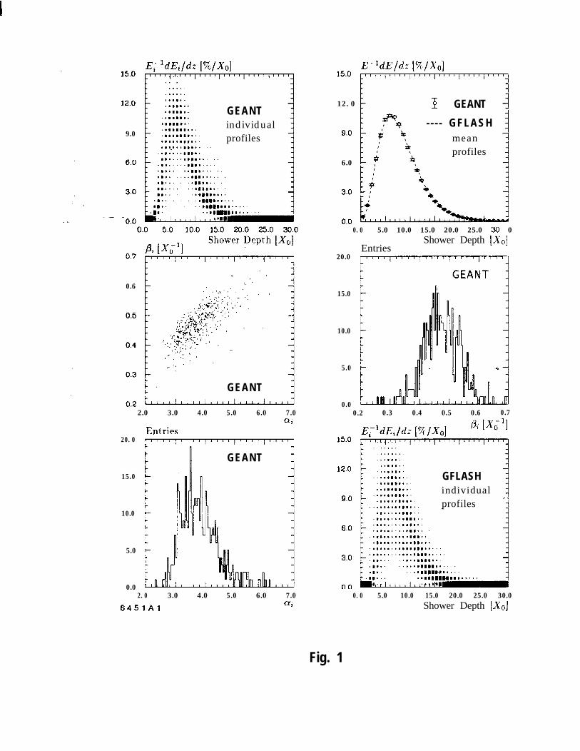
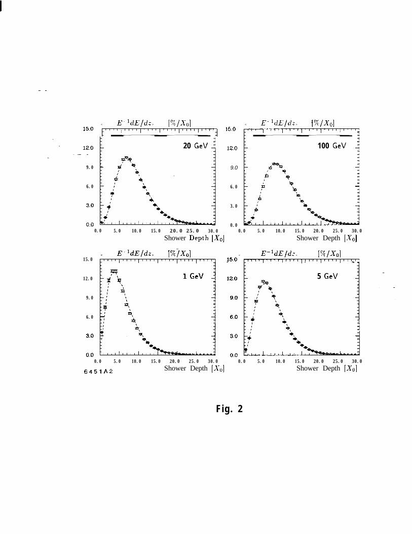
The whole procedure is presented graphically in fig. 1 for 10 GeV e- show-ers. The individual and the mean energy profiles of 400 showers, as generatedwith GEANT and with GFLASH, are shown. In addition, the distribution of
the parameters oi and pi, and their correlation as obtained from GEANT, are- - given. A comparison of the GEANT and GFLASH simulation reveals good agree-
ment in the mean profiles (additional energies are compared in fig. 2) and in theindividual fluctuations, particularly in the variation of the center of gravity andthe shower maximum.
. 3.2 -L&era1 shower profile
For the description of the lateral energy profile of electromagnetic as well ashadronic showers, we assume only a radial, and no azimuthal dependence. Theaverage radial shower distribution is frequently described by the superposition oftwo exponentials (see e.g., ref. 10). One of them describes the confined energeticcore of the shower and the other the surrounding halo.
In GFLASH, we have used the very simple ansatz
f(r) = 2rRzo --(r2 + Rijo)2 ’ (6) ‘-
for both electromagnetic and hadronic showers, which seems quite adequate, atleast as long as the lateral resolution of the calorimeter is of the order of or largerthan N 1 Moliere radius (RM) for electromagnetic and N 0.1 absorption length(X0) for hadronic showers. The radius r and the free parameter R5o in eq. (6) are in-units of RM (or X0 for hadronic showers). Fixed amounts of energy (energy spots)are deposited at radii r, generated according to the radial probability function. Tosimulate the fluctuations of individual showers, it is necessary to parameterize the
- mean and the variance (V) of the approximately log-normal distributed parameter&,o as a function of shower energy E [GeV] and hs ower depth z [in units of X0 or
x01:(&o(+)) = [RI + (& - & 1nE) zln ,
VR~~(J+) = [(Sl - & 1nE) (S3 +&z) (&o(E,~)]~ .
This parameterization, with n =’ 1 (2) for hadronic (electromagnetic) showers,
5
describes the increasingly slower growth of the radial extent and of the relativefluctuations Jo;=/ (R50 o a s) f hower with increasing energy. Lateral distributionsfor 10 GeV e- showers as a function of depth generated with GEANT and GFLASHare compared in fig. 3. As can be seen, there is reasonable agreement in the
- - description of the hard core and halo of the showers.
3.3. Sampling fluctuations
The conversion from the deposited energy to the fraction which is visible inthe active part of the sampling structure is performed during the lateral deposi-tioning of the energy spots. In addition, the sampling fluctuations are taken intoaccount.
The visible energy for a spot is computed using the measured samplingfractions Kp and the relative fraction g/Gp (and, in addition, G/Kp for hadronshowers), which may depend on the position of the spot in the calorimeter. Thesampling fluctuations are reproduced by depositing a Poisson distributed numberof spots N,(e) fo energy E, per longitudinal integration interval ! according to
the radial probability function. Assuming the energy resolution to be simulated is __
given by
udp-=-Edp
and with
(8)
we find for the spot energy:
ES=a2 .
4. Parameterization of hadronic showers
It is convenient to imagine a hadronic shower as consisting of a purelyhadronic and a r” component (mainly TO’S and some q’s).The large fluctuationsof the relative fractions of the 7rd and hadronic components in a shower lead to
6
fluctuations in a noncompensating calorimeter (e/h # l), which are much largerthan the fluctuations of electromagnetic showers alone. A simulation of hadronicshowers has to take into account:
l the energy dependence of the fraction of the 7r” component (c+) and itsfluctuation;
l the response of the calorimeter which, in general, differs for the 7r” and thepurely hadronic showers; and
l the different propagation scales, X0 for the 7r” and X0 for the hadronic-- _
component.
4.1. Longitudinal parameterisation
A well-known ansatz for the parameterization of the mean longitudinal en-ergy profile [l] uses the superposition of two Gamma distributions to describe the
7r” and the purely hadronic subprofiles:
d&j, = Edp [(l - c,o) ‘H(Z) dx + c,o E(y)&] ,
with 3-1(x) = w ) and x=hslz ?
(9) ‘-
with yae-1
E(Y) =emy
w&J ’and y = Pese *
-The distance from the shower starting point is given by sh [X0] for the ha.dronicand by se [X0] for the 7r” component.
We used this ansatz to describe the mean shower energy profile obtainedfrom a simulation of the Hl calorimeter, using GEANT. A satisfactory descriptionof the shower shapes could only be obtained if one allowed the parameter cKoto decrease with energy which is inconsistent with data [8]. This behavior hasalso been observed by fitting data with a similar method [11,12]. It is, however,necessary to correctly simulate the 7r” and hadronic subprofiles individually in orderto compute their different responses and the fluctuations of individual showersproperly. We expected an ansatz containing three terms to accomplish this:
7
- -
d-&, = fdp Einc [ch 3-1(x) da: + cf F(Y) dy + cz L( 2) dz] ,
(10)
with W(x) = .w ) and i-r = Ph [&j-l] si [X0] ;
with and Y = Pf [ql] Sf [X01 ;
-- -.with and 2 = p1 [x,y Sl [X01 .
As before, the first term describes the purely hadronic shower profile. Thesecond term models the subprofile of the 7r” fraction which is produced in the firstinelastic interaction(the index f stands for “first”). Its scale is measured in X0.The third term simulates the subprofile of the r” fraction, which is produced inthe course of the further development of the shower (the index e stands for “late”).It scales in X0. The fraction of deposited energy (fd,) with respect to the energy
.L .Dof the incident particle (Ei,c) takes the intrinsic losses during the hadronic showerdevelopment into account.
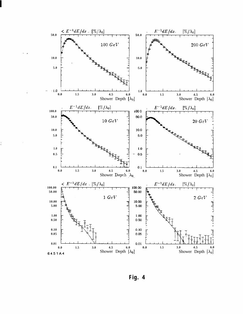
Assuming an energy dependence of the form a + b In E for the parametersto be fitted, a good description of the mean energy profile was achieved. This canbe seen in fig. 4, which shows the results of the fits to the mean shower profiles for
-different energies simulated with GEANT. However, despite this good agreement,two problems remained. One problem was that one needed two sets of parameters,one for 1 ,S Einc rS 5 and one for 5 < Einc [GeV] 35 200, and the other problem
- was that for some of the parameters a normal or log-normal distribution was nota good approximation. Both of these “defects” could be remedied by taking therelative probabilities for the occurrence of the different subprofiles into account.
4.2. 79 fluctuations
To simulate the 7r” fluctuations, it is not sufficient to just fluctuate theaverage fractions ch, cf, and cl of the deposited energy [see eq. (lo)]. The reasonsare:
8
l not every hadronic shower with energy ;S 5 GeV yields a 7r” in the firstinelastic interaction; and
l up to an energy of about 50 GeV, also no “late” 7r” may be produced.
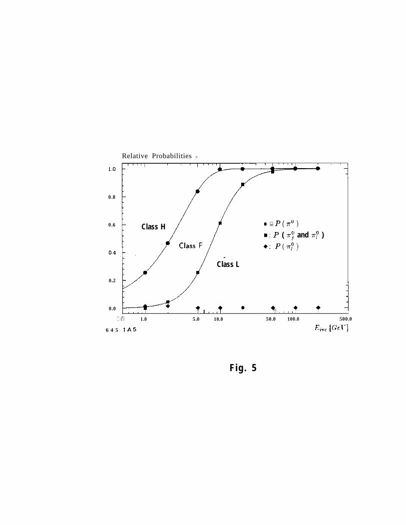
- _ In fig. 5, the relative probabilities for a hadronic shower to have any no’sP(,“), to have a my and a ri component P(xy and ri), and to have only a xjfraction P($) are shown as simulated by GEANT. We distinguish three classes ofhadronic showers according to our ansatz:
1) purely hadronic showers:-- _
class H with P(7r”) < P 2 1,
2) showers containing a 7ry component:
class F with P( 7ry and $) < P < P(,‘), and
3) showers which in addition to 7ry also contain a $ component:
class L with 0 < P < P($ and $‘),
where P is a uniform distributed random number.
Taking these probabilities into account and distinguishing between the three -,
shower classes finally allows us to successfully simulate individual hadronic showersusing eq. (10). The fractions ch , cf , and cl are calculated according to:
Ch (E) = 1 -fro (E)Cf (E) = fro (Jq (1 - fL0 W))Cl (a = fro w 20 w
(11)with Ch ( E ) + Cf (E) + Cl u9 = 1 ’
_ and fro = (2) , fro = (2) .
The energy dependence of the mean r’ fractions as obtained from GEANT are
shown in fig. 6. The fractional 7r” energy of an individual shower is then given byfro/P(ro), which is also displayed in fig. 6.
As in the case of electromagnetic showers, individual shower profiles are usedto obtain the means, fluctuations and correlations of the parameters f+ , fro , fro ,
9
crh , /?h, clef, pj, al, and pi. For shower class H, there are three; for class F, thereare six; and for class L, there are nine parameters whose means and covariancesare parameterized as a function of energy.
The vector of parameters Z for an individual shower is given by [13]
i?=ji+ccz’ ) with V=CCT . (12)
The vector Z contains maximally nine normal-distributed random numbers withvariance of one, ji is the vector of the means of the parameters and V is their covari-
. ante matrix. A method by Cholesky [14] is used to decompose the n-dimensionalsymmetric matrix V. To use the,more intuitive parameters a;i and pij instead ofthe covariance xj , it is the correlation matrix p which is decomposed in GFLASHafter the transformation V = apcrT with the diagonal matrix O.
For the simulation of the lateral shower distribution and the sampling fluc-tuations, the same functional form and basically the same method are used as forelectromagnetic showers.
-5. The GEANT-GFLASH interface
The interfacing of GFLASH with GEANT was done for the following reasons:
l Like many other experiments, the Hl collaboration has decided to use GEANTfor the description of the detector geometry in its simulation program. WithGFLASH implemented in GEANT, it is then very easy for the user to switchbetween simulations of showers using GEANT/GHEISHA [5,7] or the pa-rameteriza.tion algorithm of GFLASH. In addition, in this scheme, GEANTcan be used for the first inelastic interaction(s) (for example, until the ener-gies of the secondaries of a very high energy incident particle have cascadeddown to the energy range for which the parameterization in GFLASH hasbeen tested), switching to GFLASH for the remaining secondaries.
l When using GFLASH, it is appropriate to describe a calorimeter moduleof the same type with one medium characterized by a suitable average overthe properties of the materials of that module. This considerably reducesthe time spent by GEANT in searching for volumes and tracking.
10
l The major part of the energy of a shower is deposited inside a small cylin-der of about one RM for electromagnetic showers, and less than an X0 forhadronic showers. To a good approximation, therefore, the shower devel-
opment is determined by the medium found at the core of the shower.The “tracking” routines of GEANT are used to provide GFLASH with thegeometry and material information it needs.
In fig. 7, we show a simplified schematic of GEANT and the integration ofthe relevant GFLASH routines (underlined). A trivial change in GTVOL permitsattachment of GFLASH.
The routine GTREVE administers the tracking of the primary tracks of
the event (prim-tracks) and of the secondary tracks (set-tracks) generated dur-ing tracking by various physics processes. GTRAK, using geometry information
(geombanks), tracks particles through the different volumes. Within a given vol-ume, it is the task of GTVOL to call the particle-type specific routines for thesimulation of physical processes. These are the routines GTGAMA for photons,
GTELEC for e+ and e-, GTNEUT for neutrons, GTHADR for all other hadrons,GTMUON for p’s, and GTNINO for v’s. The- energy loss DESTEP’ calculated .-in these routines and the generated secondary particles [GKIN (5,NGKINE)I arepassed on to the user routine GUSTEP. At this point, GFLASH can be attached.If an inelastic reaction has taken place in a volume belonging to the calorime-ter, then this point is taken to be the starting point for the shower development.Whether the ensuing shower development will be parameterized or continued to besimulated in detail can be made dependent on boundary conditions determined bythe user. If the shower is to be generated by GFLASH, a “pseudoshower-particle”with the four-momentum of the incident particle (the energy is modified, depend-
ing on the incident particle type), initiating the inelastic reaction is created andstored (set-tracks). The tracking of the original particle is stopped. Standard
GEANT routines can be used to track the “pseudoshower-particle” through thedetector and to get the material parameters (X0, X0, A, 2, and RM) necessaryfor the generation of the longitudinal and lateral shower profiles. This is accom-plished by inserting one call to the GFLASH routine GTEMSH (for electromag-netic shower simulation) and one to GTHASH (for hadronic shower simulation)
I
11
into the GEANT routine GTVOL. This small change in GTVOL is the only changeneeded inside a GEANT routine.
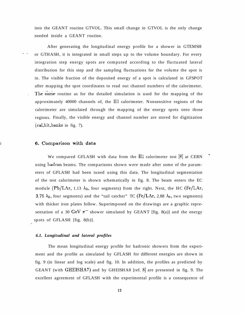
After generating the longitudinal energy profile for a shower in GTEMSH- _ or GTHASH, it is integrated in small steps up to the volume boundary. For every
integration step energy spots are computed according to the fluctuated lateraldistribution for this step and the sampling fluctuations for the volume the spot isin. The visible fraction of the deposited energy of a spot is calculated in GFSPOTafter mapping the spot coordinates to read out channel numbers of the calorimeter.
. The-s&e routine as for the detailed simulation is used for the mapping of theapproximately 40000 channels of, the Hl calorimeter. Nonsensitive regions of thecalorimeter are simulated through the mapping of the energy spots onto thoseregions. Finally, the visible energy and channel number are stored for digitization
(Cal-hit-banks in fig. 7).
6. Comparison with data
We compared GFLASH with data from the Hl calorimeter test [8] at CERN .q
using hadron beams. The comparisons shown were made after some of the param-eters of GFLASH had been tuned using this data. The longitudinal segmentationof the test calorimeter is shown schematically in fig. 8. The beam enters the EC
module (Pb/LAr, 1.13 X0, four segments) from the right. Next, the HC (Fe/LAr,_ 3.76 X0, four segments) and the “tail catcher” TC (Fe/LAr, 2.88 X0, two segments)
with thicker iron plates follow. Superimposed on the drawings are a graphic repre-sentation of a 30 GeV 7r- shower simulated by GEANT [fig. 8(a)] and the energy
_ spots of GFLASH [fig. 8(b)].
6.1. Longitudinal and lateral profiles
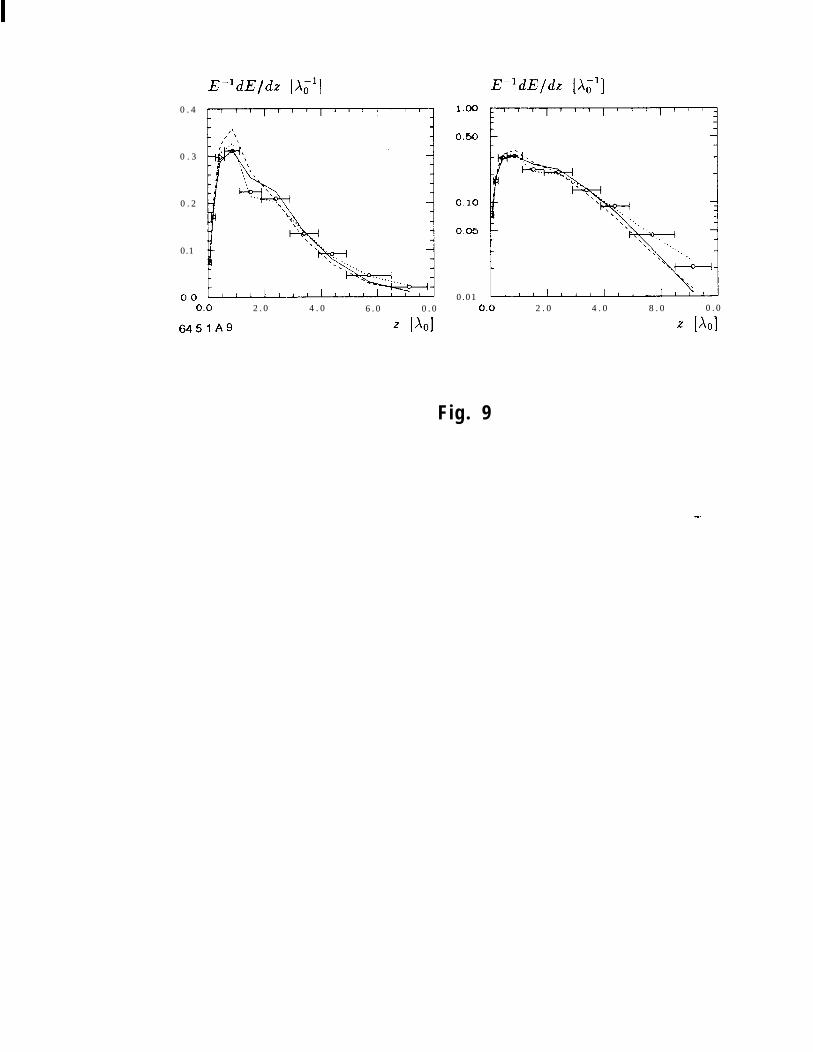
The mean longitudinal energy profile for hadronic showers from the experi-ment and the profile as simulated by GFLASH for 1d’fferent energies are shown in
fig. 9 (in linear and log scale) and fig. 10. In addition, the profiles as predicted byGEANT (with GHEISHA’I) and by GHEISHA8 [ref. 81 are presented in fig. 9. Theexcellent agreement of GFLASH with the experimental profile is a consequence of
12
the refitting of some of the GFLASH parameters. Figure 10 shows the develop-ment of a second maximum in the segment HC2 with increasing energy which iswell-simulated by GFLASH. This effect can be understood as follows. The lengths(in X0) of ECJ, HCr, and HC2 increase such that roughly equal numbers of show-
-. -ers are starting in these segments. However, in units of X0, due to the differencein the ratios of X0 to X0 for Pb and Fe, the segment HCr is shorter than the neigh-boring segments. While an electromagnetic subshower of a few GeV starting in
EC4 or HC2 will be almost completely contained there, such a subshower startingin HCr will leak some of its energy into HC2. The correct simulation of this effect-- _
-. by GFLASH indicates a good parameterization of the 7ry fraction of the shower.
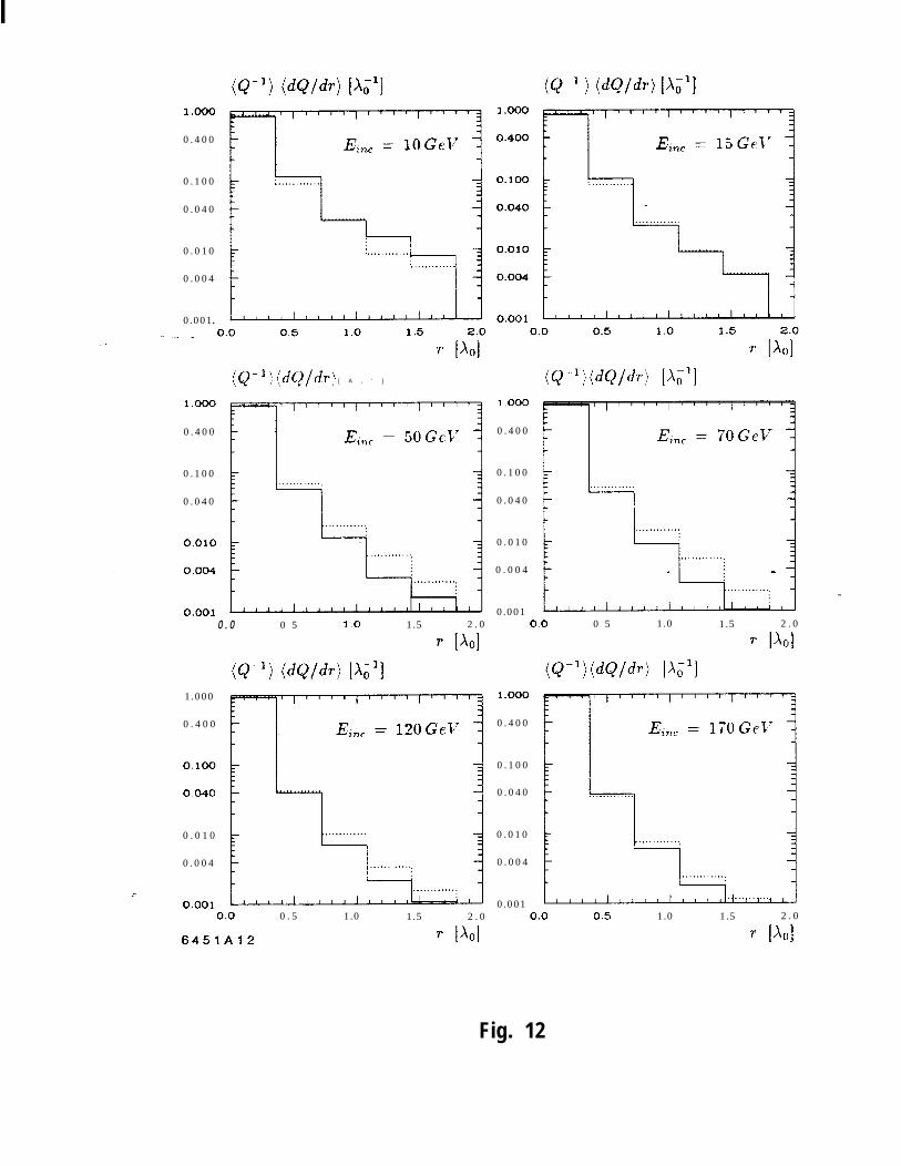
The dependence of the mean lateral profile on the shower depth and energycan be seen in fig. 11 where the lateral charge distribution as a function of depthis shown for one energy, and in fig. 12 where it is plotted for different energies ata fixed depth. There is good agreement between GFLASH and the experiment forthe core as well as the halo of the shower.
6.2. Fluctuations of hadronic showers.- .m
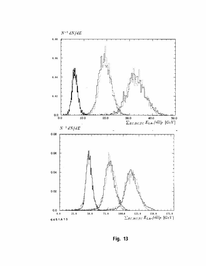
The total visible energy for the modules EC, HC, and TC (normalizedto their respective sampling fractions for minimum ionizing particles) for sixdifferent beam energies is compared with the expectations from GFLASH in fig. 13.For the energy range considered, the agreement is good and the asymmetry ofthe distributions, which is expected for noncompensating calorimeters, is properlysimulated. In this comparison of experimental and simulated data, only a sin-gle constant relating charge to energy as obtained experimentally with muons wasused, and not-as is frequently done-a set of constants which is determined by
_ demanding equality of the means with the incident energy and minimal variances.
The energy resolution of the calorimeter is shown in fig. 14 for pions asa function of energy, together with the results from the simulation. The goodagreement here suggests that the intrinsic and sampling fluctuations for the Pband Fe calorimeters are properly taken into account in GFLASH.
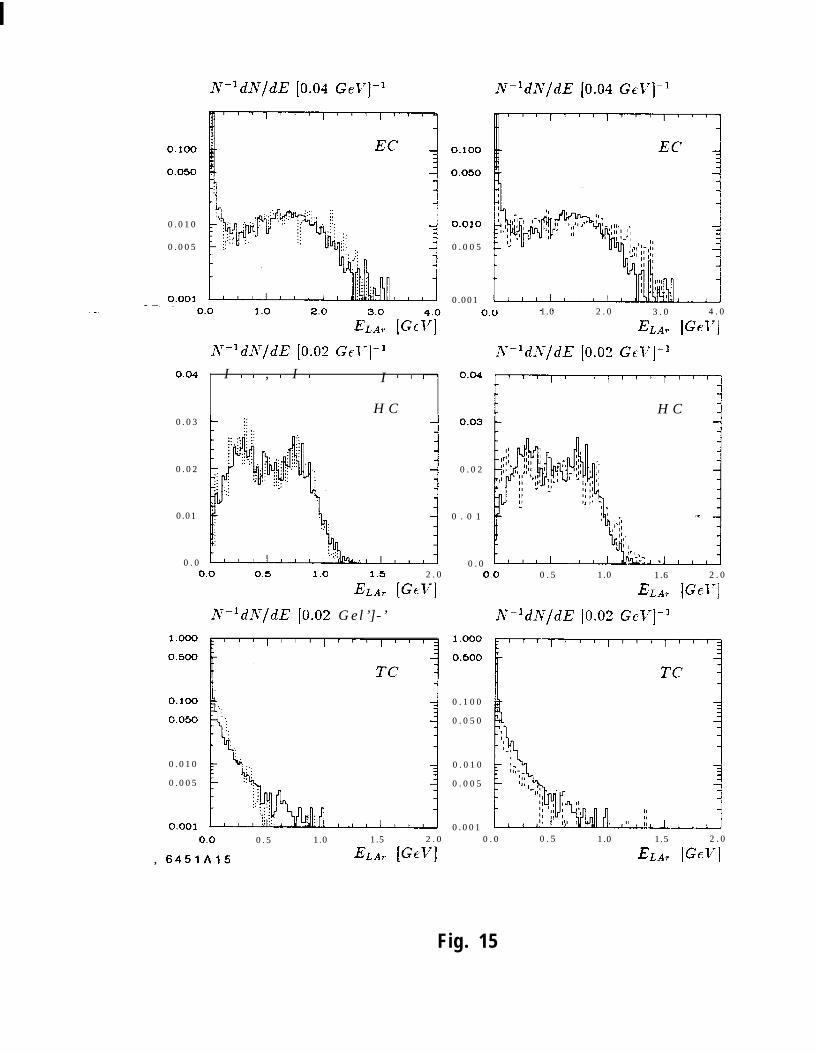
The visible energy seen in the three different modules (EC, HC, and TC) for30 GeV showers is compared in fig. 15 with results from GEANT and GFLASH.
13
The good agreement observed for GFLASH indicates a proper handling of thedifferent materials and sampling structures in the simulation. The pattern of
slightly too much energy in EC and too little in TC, as generated by GEANT, isa consequence of the shower length of GEANT being too short, as can be noticed
- _in fig. 9.
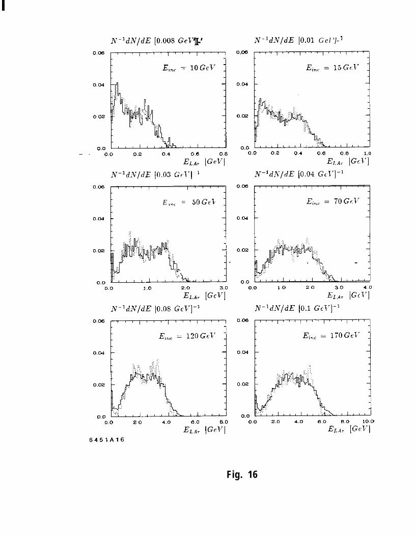
The first maximum seen in the visible energy in HC is due to showers startingin EC and depositing most of the ~7 energy there, while the second maximum isdue to showers originating in HC. How the visible energy distribution for the HCchanges-as a function of energy and how this is simulated by GFLASH is shownin fig. 16.
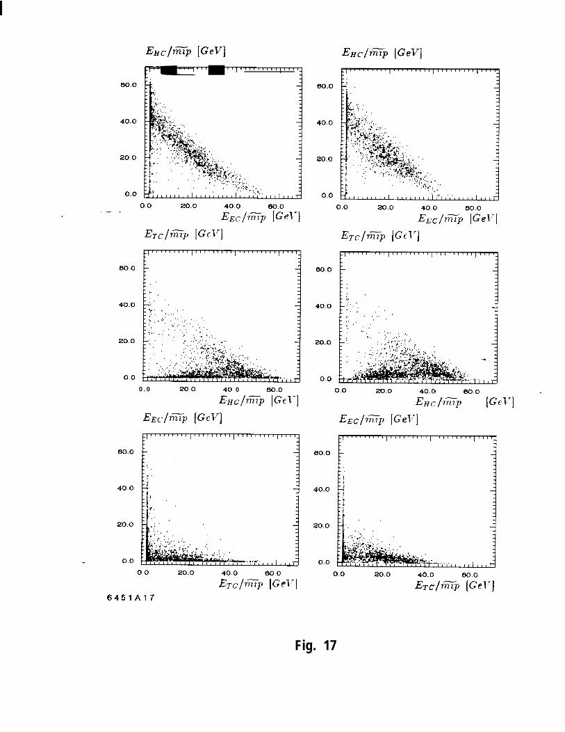
The energy fluctuations and correlations for different calorimeter segments
are displayed in fig. 17 for 70 GeV showers. The agreement between GFLASH andthe data is quite satisfactory, even for the “long range” (EC vs. TC) correlations.
7. Speed estimate
We used the Hl detector simulation program [15], which is still under devel-.- .*opment, to provide some preliminary timing information. We took as an example50 GeV pions which shower in the Hl forward calorimeter [9]. We found the fol-lowing average times [using an IBM 3090-1503 (M 3.5 VAX 8600)]: 85 ms for thetracking of the pion from the interaction point through the central and forwardtracker volumes to the first inelastic interaction in a calorimeter volume (GEANT),
- 55 ms for the tracking of the “pseudoshower-particle” (GEANT), and 30 ms forthe generation of the energy spots (GFLASH). This indicates that, at least in thecontext of Hl? the time spent on the shower-specific tasks of GFLASH is small com-
_ pared to the time spent on the geometry-specific tasks of GEANT. The 30 ms forGFLASH includes the time for the tracking of a shower within a volume which isdone by GFLASH. Compared to a detailed simulation using GEANT/GHEISHAwith standard values for the cutoff energies, we found that the simulation withGFLASH is about 180 times faster. Since neither the detailed nor the parameter-ized simulation, as such, were particularly optimized for speed, the numbers givenabove should be taken with caution.
14
A simulation of the Hl test calorimeter (as shown in fig. 10) by GFLASHand GEANT/GHEISHA leads to the CPU time requirements (using an IBM 3090-180E) as given in Table 1. The times given for GFLASH depend on the parame-
terization chosen for the number of energy spots as a function of energy, which in- _turn depends on the geometry and size of the readout channels. In-this example,200 (250) p ts o s were generated for 50 (200) GeV.
Perhaps more important in the comparison of the time required for the de-tailed and parameterized simulation of showers is their energy dependence. Dueto theproportionality of energy and total track length of a shower, the computer_time required for simulation with GEANT/GHEISHA increases linearly with en-ergy, while for GFLASH the time’is proportional to the shower length which growsonly logarithmically with energy.
8. Conclusions
GFLASH” provides a realistic and fast parameterization for the simulationof electromagnetic and hadronic showers in a geometry defined by the user withGEANT. The longitudinal and lateral distribution, their fluctuations and correla- .*tions, are modeled in a consistent way. For hadrons, this was made possible bya new ansatz for the longitudinal energy profile consisting of three Gamma dis-tributions: one for the purely hadronic component of the shower, one for the 7~’fraction originating from the first inelastic interaction, and one for the 7r” frac-
tion from later inelastic interactions. The interfacing of GFLASH with GEANTprovides great flexibility and ease of use.
Acknowledgments
We are very much indebted to H. Greif for providing us with data tapesand information from the Hl calorimeter test at CERN. We also thank T. Hansl-Kozanecka and D. Groom for their careful reading of this manuscript. One of us(G. G.) would like to thank the SLAC directorate and M. Per1 for the hospitalityhe is enjoying at SLAC.
O GFLASH is available for distribution; please contact one of the authors.
15
References
[l] R. K. Bock et al., Nucl. Instr. and Meth. 185 (1981) 533;M. della Negra, Scripta Phys. 23 (1981) 469-479.
[2] E. Longo and I. Sestili, Nucl. Instr. and Meth. 128 (1975) 283.- _[3] Y. Hayashide et al., CDF Note 287, Batavia, IL (1985).
[4] J. Badier and M. Bardadin-Otwinowska, ALEPH 87-9, EMCAL 87-1, Geneva(1987).
[5] R. Brun et al., GEANT3 User’s Guide. CERN-DD/EE 84-1, Geneva (1986).
_ [6] -M. Rudowicz, Diplomarbeit an der Universitat Hamburg; MPI-PAE/Exp. El. 200(1989);S. Peters, Diplomarbeit an der Universitat Hamburg; MPI-PAE/Exp. El. 202(1989).
[7] GHEISHA7 as implemented in GEANT; see also H. C. Fesefeldt, PITHA Re-port 85/02, RWTH Aachen (1985).
[8] Hl Calorimeter Group (W. Braunschweig et al.), DESY 89/022 (1989).
[9] Hl C 11 bo a oration, Technical Proposal for the Hl Detector, DESY, Hamburg,1986.
[lo] G. A. Akopdjanov et al.,NucI. Instr. and Meth. 140 (1977) 441-445. ,_
[ll] E. Hughes, CERN CDHS Internal Note 4, Geneva (1986).
[la] W. J. Womersley et al., Nucl. Instr. and Meth. A267 (1988) 49, and erratumA278 (1989) 447.
[13] F. James, Rep. Prog. Phys. 43 (1980) 1145-1189.
[14] R. Y. R b tu ins ein, Simulation and the Monte Carlo Method (John Wiley &Sons, New York, 1981).
[15] G. D. Pate1 et al., Hl Collaboration Internal Note, Hamburg (1988).
16
Table 1. CPU time requirements (IBM 3090-180E) for the simulation of show-ers in the Hl test calorimeter.
Energy GFLASH GEANT
7r+ 50 GeV 26 ms 8s-. _7r+ 200 GeV 31 ms -32 s
e- 50 GeV 10 ms 30 s
e- 200 GeV 11 ms 110 s
17
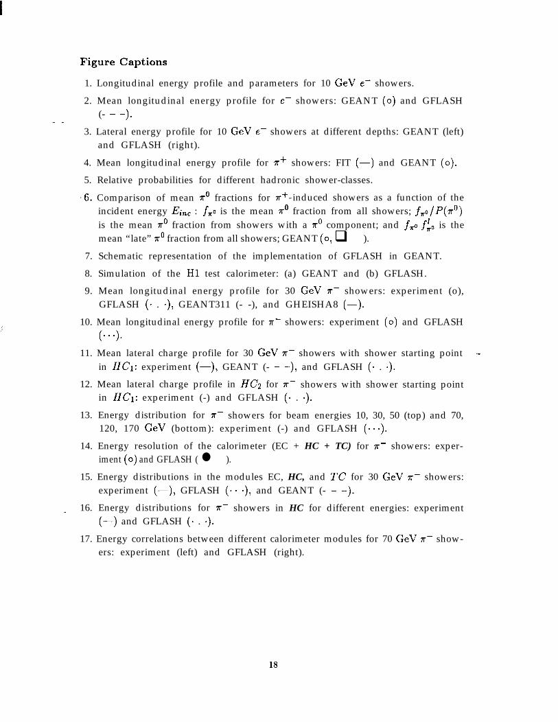
Figure Captions
1. Longitudinal energy profile and parameters for 10 GeV e- showers.2. Mean longitudinal energy profile for e- showers: GEANT (0) and GFLASH
(- - -).- -3. Lateral energy profile for 10 GeV e- showers at different depths: GEANT (left)
and GFLASH (right).4. Mean longitudinal energy profile for 7r+ showers: FIT (-) and GEANT (0).5. Relative probabilities for different hadronic shower-classes.
.6. Comparison of mean 7r” fractions for 7r+- induced showers as a function of theincident energy Einc : fxo is the mean w” fraction from all showers; fxo/P(ro)
is the mean no fraction from showers with a r” component; and fro fLo is themean “late” r” fraction from all showers; GEANT (0, q ).
7. Schematic representation of the implementation of GFLASH in GEANT.8. Simulation of the Hl test calorimeter: (a) GEANT and (b) GFLASH.9. Mean longitudinal energy profile for 30 GeV 7rr- showers: experiment (o),
GFLASH (. . m), GEANT311 (- -), and GHEISHA8 (-).
,: 10. Mean longitudinal energy profile for X- showers: experiment (0) and GFLASH(. * *).
11. Mean lateral charge profile for 30 GeV 7rr- showers with shower starting point .qin HCl: experiment (-), GEANT (- - -), and GFLASH (. . a).
12. Mean lateral charge profile in HC;! for 7~~ showers with shower starting pointin HCl: experiment (-) and GFLASH (. . e).
13. Energy distribution for r- showers for beam energies 10, 30, 50 (top) and 70,120, 170 GeV (bottom): experiment (-) and GFLASH (...).
14. Energy resolution of the calorimeter (EC + HC + TC) for 7rr- showers: exper-iment (0) and GFLASH ( l ).
15. Energy distributions in the modules EC, HC, and TC for 30 GeV 7rr- showers:experiment (-), GFLASH (0. o), and GEANT (- - -).
_ 16. Energy distributions for K- showers in HC for different energies: experiment(-) and GFLASH (. . s).
17. Energy correlations between different calorimeter modules for 70 GeV 7r- show-ers: experiment (left) and GFLASH (right).