MSc Thesis in Finance
The Feasibility of Optimal Currency
Area for ASEAN after adopting the
ASEAN Economic Community
Blueprint in 2008
Does it facilitate the region to move closer to a single currency area?
Author: Thian Thiumsak
Supervisor: Martin Strieborny
Lund University
Department of Economics
Date: May 27th 2014
1
Abstract
This paper investigates the feasibility of OCA for ASEAN after the implementation of
ASEAN Economic Community Blueprint in 2008. Dynamic Conditional Correlation (DCC)
model with and without a structural break are used to identify whether the policy
implemented facilitates the region to move closer to a single currency area. Industrial
production index growth rate and change in short-term interest rate for ASEAN founders
(Indonesia, Malaysia, Philippines, Singapore, and Thailand) from the period of 2001-2013
are selected as a proxy for OCA and Maastricht criteria respectively, which are cited as
significant factors for successful functioning of OCA. The results show that there is a
structural break for most conditional correlation of country pairs of the two variables after the
implementation of integration policy in 2008 and that most of the conditional correlations
decrease over time. The results imply that the whole region diverges away from OCA and
Maastricht criteria and that the feasibility of OCA is decreased. As discussed by a number of
previous researches regarding the issue, there is a possibility that higher economic integration
resulted from integration policy may cause economic divergence due to specialization in
industry of country members. For higher effectiveness of future integration policy
formulation, a formal quantitative testing is required in order to precisely identify that higher
economic integration causes higher specialization in the industry and, hence, more
divergence in business cycle.
2
Contents 1. Introduction ......................................................................................................................................... 3
2. Literature Review ................................................................................................................................ 5
2.1 OCA Criteria explained ................................................................................................................ 5
2.1.1 Early Development of Optimal Currency Area (OCA) theory .............................................. 5
2.1.2 New development of Optimal Currency Area (OCA) theory ................................................ 8
2.2 Maastricht Criteria explained ...................................................................................................... 11
2.3 Conclusion Concerning OCA and Maastricht Criteria ............................................................... 11
2.4 Operationalizing the OCA Criteria ............................................................................................. 12
2.4.1 An OCA Index ..................................................................................................................... 12
2.4.2 Generalized-Purchasing Power Parity Analysis ................................................................... 13
2.4.3 Structural Vector Autoregression (SVAR) .......................................................................... 13
2.4.4 Correlation and Cluster Analysis ......................................................................................... 13
2.5 Major ASEAN Studies ................................................................................................................ 14
3. Integration Indicators and Analysis .................................................................................................. 16
4. Methodology ..................................................................................................................................... 18
5. Data ................................................................................................................................................... 22
5.1 Choice of variables ..................................................................................................................... 22
5.2 Descriptive Statistics ................................................................................................................... 23
.............................................................................................................................................................. 25
6. Empirical Results .............................................................................................................................. 25
6.1 Structural Break and Integration Policy ...................................................................................... 25
6.2 Dynamic Conditional Correlation with a Structural Break ......................................................... 28
7. Conclusion ........................................................................................................................................ 31
8. References ......................................................................................................................................... 33
9. Appendices ........................................................................................................................................ 36
3
1. Introduction
After the introduction of the Euro in January 1999, there has been much interest in monetary
integration by both academics and policy-makers. In the case of Southeast Asia, a key
historical event which led to an initiative of a common currency is the currency crisis of
1997/98, which developed to become one of the worst economic crises of the region. The
currency crisis has decreased the credibility of unilateral fixed exchange rate and increased
the attention of more solid pegs, for instance currency boards, using some country’s currency
as domestic currency and common currency arrangement (Bayoumi and Mauro 2001).
When considering the adoption of a common currency, it is inevitable for countries involved
to face a tradeoff. Major advantages of single currency area include price and exchange
stability, increases in intra-regional trade, elimination of transaction cost, among others.
Nevertheless, there is no “free lunch” to any kind of economic decisions and adoption of a
common currency is not an exception. The key disadvantage of monetary integration is the
loss of control in nation’s monetary policies (i.e. policy flexibility) to balance the economic
disequilibrium from macroeconomic shocks.
Nevertheless, the cost of moving to monetary union can be reduced through a number of
prerequisites deemed as being essential: (1) high degree of factor mobility, (2) openness of
the economy and size of the economy, (3) product diversification, (4) similarity of inflation
rate, (5) price and wage flexibility, and (6) the need for exchange rate variability.
In the case of ASEAN1
, monetary integration is one of the main objectives of the
development plan for ASEAN called “ASEAN Vision 2020”. To reach the goal of a common
currency, higher economic integration is the key element. This reason is a significant driver
for the ASEAN leaders to agree and form ASEAN Economic Community (AEC) by 2015
which transforms ASEAN into a region with free movement of goods, services, investment,
skilled labor, and free flow of capital.2
After the agreement, each country in the region has adopted the ASEAN Economic
Community Blueprint (AECB) established during the regional meeting in 2007 as a guideline
towards establishment of AEC. The key elements of the Blueprint includes (1) tax on most
imported goods from ASEAN countries will be completely exempted (2) Foreign Direct
1 ASEAN stands for The Association of South East Asia Nations, which include 10 countries: Brunei Darussalam,
Cambodia, Indonesia, Lao PDR, Malaysia, Myanmar, Philippines, Singapore, Thailand, and Vietnam. 2
Yong, Ong K. “Towards ASEAN Financial Integration.” 18 February 2004. <http://www.asean.org/resources/2012-02-10-
08-47-56/speeches-statements-of-the-former-secretaries-general-of-asean/item/towards-asean-financial-integration>
4
Investment (FDI) within ASEAN is more liberalized and (3) higher free flow in skilled labor
among ASEAN countries.3
As a consequence, the region’s economy is expected to be more and more integrated during
the preparation towards AEC as there will be higher factor mobility and intra-regional trade
induced by AECB.
The purpose of this paper is to investigate the feasibility of OCA for ASEAN after the
implementation of AECB in 2008 (i.e. integration policy). The main research question is to
answer whether the preparation towards AEC, which expects a higher economic integration,
facilitates the region to move closer to a single currency area. Dynamic Conditional
Correlation (DCC) model with and without a structural break is used to examine the
evolution of ASEAN countries’ two macroeconomic variables: industrial production index
and short-term interest rate. The selection of variables is based on OCA and Maastricht
criteria and previous papers regarding OCA for ASEAN.
This paper contributes to the literature of the feasibility of OCA for ASEAN in two aspects.
First, it updates the picture of the possibility of OCA for ASEAN after the most recent
political attempt concerning economic integration of the region. Information regarding the
development of convergence for ASEAN as a whole as well as individual country can be
useful in formulating effective future policy for promoting further economic integration.
Secondly, the Dynamic Conditional Correlation (DCC) model is used to examine OCA issue
in this paper. There are a number of reasons to justify the selection of this methodology over
the others.
First of all, since an objective of this paper is to investigate the movement of economic
variables across sample countries in order to identify to what extent ASEAN converges to a
single currency area, methodology that is relevant to answer this research question must
exhibit convergence and divergence of comovement of variables over time. Since the DCC
model allows correlation of economic variables to be time-varying, it is suitable to apply this
model to examine OCA issue in this paper. Secondly, among methodologies that allow
comovement of economic variables to be time-varying, DCC model has been proved to be
more accurate than other types of estimation such as simple multivariate GARCH and
moving average (Robert Engle 2002). Thirdly, this methodology has been widely used not
3For more on the information of ASEAN Economic Community Blueprint and its strategic schedule see ASEAN
Economic Blueprint (2008)
5
only in financial area but also in economic application such as the paper by Jim Lee (2005)
which examines the comovement of output and price of the US over time.
The paper is organized as follows. Section 2 reviews theoretical progress and empirical
methodologies to execute OCA theory. Section 3 analyzes the relevant integration indicators
as a way to obtain preliminary idea regarding convergence development of OCA for the
region. Section 4 explains and describes the DCC model. Next, brief description of data
employed in this paper is presented in section 5. Finally, the paper is concluded in section 6.
2. Literature Review
2.1 OCA Criteria explained
2.1.1 Early Development of Optimal Currency Area (OCA) theory
2.1.1.1 High Degree of Factor Mobility
The theory of Optimal Currency Area (OCA) was primarily discussed by the work of
Mundell (1961). The literature asked an important question regarding the domain of the
currency area i.e. which countries should be included in the monetary union. Mundell argues
that the main criteria necessary for OCA is high degree of factor mobility. He explained his
argument through hypothetical example of changes in consumption pattern between two
countries and regions (i.e. a country or region respond to macroeconomic shocks
differentially or asymmetrically) under assumption that price is sticky and central bank acts
to prevent inflation. If the shift in demand corresponds with national and currency
boundaries, for an instance an increase in demand for product in country B compared with
product in country A, then a flexible exchange rate between the two individual currencies
would adjust to maintain the external and internal balance of both countries, relieving
unemployment in country A and restraining inflation pressure in country B.
Nevertheless, if the shift in demand does not correspond with national and currency
boundaries i.e. the shift is between the regions within the countries, then the flexible
exchange rate would only serve to maintain the external balance between the two countries
but not between the two regions. Hence, a region with higher demand would experience trade
surplus and inflation and a region with lower demand would experience trade deficit and
unemployment. Monetary authority in each country can pursue monetary policy to relieve
inflation in a region with higher demand at the expense of higher unemployment in a region
6
with lower demand or vice versa. Alternatively, the inflation-unemployment burden can be
shared between the two regions.
The main result of this illustration is to show that the Optimal Currency Areas are the two
regions. With separate currency, flexible exchange rate would permit external and internal
balance between the two regions. As a consequence, it can be show that factor mobility
(primarily labor mobility) can keep internal and external balance when there is a shift in
demand between the two regions. It takes place when labor migrates away from deficit region
to surplus region, concurrently relieving unemployment and wage-inflation respectively.
This argument brings about one of the Mundell’s main conclusion that factor mobility
(mainly labor mobility) can replace a system of individual regional currencies as it has the
capability to maintain internal and external balance among regions within a multi-regional
currency area. Therefore, the cost of switching to single currency is lower the higher the level
of factor mobility.
2.1.1.2 Openness and Size of the Economy
McKinnon (1963) developed further the idea of optimum size of the domain of currency area
by considering two key criteria: openness and size of the economy. In case where economies
are comparatively open (i.e. the ratio of tradable to non-tradable goods is high), flexible
exchange rates have a significant effect on internal price-level stability when devaluation
increases the cost of tradable. Since a relatively open economy with flexible exchange rate
may be able to satisfy the objectives of employment maximization and external balance but
the increase in cost of tradable goods would affect the internal price-level stability. Thus, the
opportunity cost of giving up flexible exchange rate system for a single currency is lower the
more open the economy is.
As a result to the previous criteria, the smaller the size of the economy, the more open it is
likely to be and, therefore, the lower the cost of switching to monetary union.
2.1.1.3 Product Diversification
Taking into account the works of Mundell (1961) and McKinnon (1963), Kennen (1969)
came up with product diversification as another important structural precondition to find out
if a region would be well suited for an OCA. A well-diversified country would be more
insulated to different kind of shocks than less-diversified country and, therefore, less
dependent on exchange rate movement for external adjustment.
7
Other characteristics, which also deemed to be relevant for selecting the potential countries in
an OCA, are (1) similarity of inflation rate, (2) price and wage flexibility, and (3) the need for
exchange rate variability.
2.1.1.4 Similarity of Inflation Rate
According to Fleming (1971), when inflation rates between countries are convergent, an
external balance (i.e. current account) is more likely to be achieved within the currency area
than if inflation rates are divergent. As a consequence, similarity of inflation reduces the need
of exchange rate movement and, thus, the cost of moving to monetary integration.
2.1.1.5 Price and Wage Flexibility
When there is a high flexibility of price and wage between countries, the disequilibrium
resulted from the shift in demand is less likely to be associated with unemployment in one
country and inflation in another country. As a consequence, the need for exchange rate
movement is lessen and, thus, the loss created by switching to monetary integration is
reduced (Freidman 1953 and Kawai 1987).
2.1.1.6 The Need for Exchange Rate Variability
The exchange rate acts as a shock absorber. If there has been little cause for deviation in the
exchange rate then there is not much to lose when countries move to monetary union. Thus,
the cost of adopting monetary integration is lessened (Vaubel 1976 and 1978).
2.1.1.7 Summary Concerning Early Development of OCA Theory
The early works concerning the theory of OCA appear to point out that (1) flexible exchange
rate is an adjusting variable for maintaining internal and external balance (Meade 1955) (2)
the cost of adopting a common currency is the inability for a country to use exchange rate
movement to adjust to asymmetric shocks and higher asymmetry of shocks increases such
cost and (3) the cost of switching to monetary union can be reduced through adjustment
mechanism discussed above (i.e. OCA criteria).
Particularly, the benefits implicitly assumed by the early literatures include “reductions in
transactions costs and exchange rate uncertainty, increased liquidity and trade, economies of
scale regarding currency reserves, and improvement in allocation efficiency” (Paul Duncan
Adams 2005).
8
2.1.2 New development of Optimal Currency Area (OCA) theory
The theory of OCA has been transformed in line with important theoretical developments in
other areas of economic, which seek to clarify the benefits and costs of joining single
currency area. Compared with earlier works regarding monetary union, the new OCA theory
points out that there are rather fewer costs and relatively more benefits in the adoption of
monetary integration. These developments include the vertical Phillips Curve and policy
ineffectiveness, time consistency and credibility, the role of exchange rate disputed, positive
effect of monetary union on trade, and the endogeneity of OCA criteria.
Despite less emphasized in the formal theory of optimal currency area, similar level of
economic development and similarity of financial systems are another two criteria that may
have an influence on selecting countries into a common currency area (Bayoumi and Mauro
2001).
2.1.2.1 The Vertical Phillips Curve and Policy Ineffectiveness
The traditional OCA theory assumes that flexible exchange rate would permit a country to
employ independent monetary policy in order to achieve the desired trade-off between
inflation and unemployment, as suggested by Phillips Curve. Hence, it would exert a cost
using monetary integration as countries are unable to adjust the economy to the desired
balance of inflation and unemployment. This permanent trade-off between inflation and
unemployment has been undermined by a number of developments.
Lucas (1972) and Friedman (1968) claim that monetary policies are ineffective in managing
unemployment in the long-run. The shape of long-run Phillips Curve is vertical since
unemployment is associated with the Natural Rate of Unemployment (NRU). Therefore,
inflation can be managed without negative effects on the level of long-run unemployment.
Given that monetary policy is ineffective in balancing unemployment and inflation in the
long-run, the costs of using single currency are decreased.
Nevertheless, there are a number of issues associated with the idea of monetary neutrality and
currency unions that are worth discussing when considering monetary integration. Frenkel
and Goldstein (1986) point out possible political tension that could emerge from symmetric
monetary systems (i.e. member countries cooperate in reaching policy solutions) under
conditions of asymmetric shocks. In addition, De Grauwe (1992) also shows how asymmetric
monetary system (i.e. one member country take a leadership role in setting policy) worsen the
domestic business cycle in other member countries.
9
Artis (1991) argued that the production of member countries in single currency area will be
more specialized, increasing the vulnerability of countries within the area to asymmetric
shocks.
2.1.2.2 Time Consistency and Credibility
While traditional OCA theory suggested similarity of inflation rates as a precondition for the
arrangement of single currency area, new theory shows how monetary integration could be
more beneficial when the divergence of inflation rates is high. The high inflation country
could accomplish low inflation without any cost by allowing the low inflation central bank,
which adopts a credible policy stance of optimal inflation, to take control. This result is
essentially based on the debate between discretionary and fixed policy rule.
Barro and Gordon (1983) demonstrated that central bank must pursue time consistent policy
rule in order to gain credibility. Discretionary policy, determined in each time period, creates
incentives for surprise inflation to decrease short-run unemployment level. However, such a
decline comes at an expense of increase in inflation and lack of credibility in the long-run.
The problem of time inconsistency can be solved by pursing a system of policy rule that the
economic agent perceive to be either fixed or the cost of reneging from those rules outweigh
the benefit from surprise inflation.
De Grauwe (2002) showed that Barro and Gordon’s argument could also be applied to
exchange rate policy. The promise to maintain fixed exchange rate will be credible only if the
cost of breaking that promise exceeds the gain from pursing surprise devaluation.
The arguments discussed above have in-depth implications for OCA theory as monetary
union incorporates a set of policy rules that “tie the hand” of domestic central bank
authorities in terms of monetary and exchange rate policy. As a consequence, the loss of
policy control in those countries would be considered beneficial as they will be able to attain
lower inflation rate over the long-run, without any loss of unemployment.
2.1.2.3 The Role of Exchange Rate Disputed
With the development of the asset model of exchange rate determination had led recent works
on the exchange rate to believe that, while movement in the exchange rate serve to maintain
internal and external balance, the correction is imperfect and takes a longer period than
assumed in the flow model of traditional OCA theory (Krugman 1991). This argument
regarding the exchange rate has an implication for OCA theory that the loss of exchange rate
10
as policy tool may be less costly than initially thought. There are a number of models that
associated in the argument such as the portfolio-balance model, exchange rate and Ricardian
equivalence, and the ‘sunk cost’ model.
Since exchange rate volatility has a negative effect on trade, its removal has been cited
throughout the earlier literature as a benefit of monetary union. However, recent papers argue
that the belief is overestimated. De Grauwe (2000) demonstrated that reducing exchange rate
uncertainty shifts the risk to another area of the economy by using an IS-LM model.
Moreover, the paper emphasizes that despite the fact that monetary integration, which result
in exchange rate certainty, would decrease risk, this effect would only have a one-off gain to
economic growth as indicated by Neoclassical theory and was used in ‘One Money, One
Market’ report (EC 1990).
In conclusion, the costs of monetary union have been reduced as lags in the effects of
movement of exchange rate decrease their effectiveness. In contrast, the gain from monetary
integration due to exchange rate certainty seems to be overestimated by the earlier works of
OCA theory.
2.1.2.4 Positive Effect of Monetary Union on Trade
Later papers regarding OCA produce empirical works about the positive effect of currency
union on member countries’ trade. Rose (2000) demonstrates that trade between two
countries that have the same currency is 200% bigger than trade between countries that have
different currencies by using a gravity model. This paper’s result is consistent with other
studies of the impact of currency union on trade such as Flandream and Maurel (2001), Lopez
Cordova and Meissner (2001) and Frankel and Rose (2002) which demonstrate an increase in
trade of 220, 100, and 290%, respectively.
2.1.2.5 Endogeneity of OCA Criteria
In contrast with traditional OCA theory, Frankel and Rose (1997) assert that many structural
preconditions for monetary integration proposed by traditional theorists could be supported
by the establishment of monetary union. They believed that higher economic integration
(most notably customs, monetary integration, higher factor mobility and trade integration)
increases convergence among countries. Therefore, the cost in terms of loss of exchange rate
control when switching to monetary union is reduced.
11
On the other hand, Krugman (1993) argued that increased economic integration increases the
possibility of asynchronous income fluctuation among nations. He believed that countries
would be more specialized which increases rather decreases the divergence of shocks among
the countries. As a consequence, the cost of adopting single currency in a particular region is
higher.
Nevertheless, a number of researches have a tendency to support Frankel and Rose’s (1997)
argument for the countries that have been examined, particularly the European Union. Artis
and Zhang (1995) confirmed that higher trade among members of the European Monetary
System brings about a more synchronous business cycle.
2.2 Maastricht Criteria explained
The Maastricht Treaty, which was established in 1991, identifies a required set of criteria
needed to be accomplished for countries to become a member of European Monetary Union
(EMU). The main objective of the Treaty is the convergence of both nominal and fiscal
aspects which will guarantee the convergence of monetary and fiscal policy. “In formal
terms, the criteria for nominal convergence say that a country must have an inflation rate
within 1.5% of the average inflation rate of the three members with the lowest inflation rates
and a long-run bond yield within 2% of the average of the bond yields of the same three
countries. Furthermore, the Treaty requires that the exchange rate must have been stable
within the plus or minus 15% ERM bounds for at least two years. As regards fiscal policy,
the budget deficit should be no higher than 3% of the GDP and public debt less than 60% of
the GDP” (Boreiko 2003).
2.3 Conclusion Concerning OCA and Maastricht Criteria
In conclusion, the main reason that both OCA and Maastricht criteria, which represent real
convergence and nominal convergence (i.e. policy convergence), are required to be fulfilled
is because they are considered to be the significant conditions for successful functioning of
monetary union. It has been argued that while countries in European Union were converging
in Maastricht criteria before joining the EMU, a few countries were converging in OCA
criteria. In fact, some are even reported to show divergence. As a result, countries whose
preconditions are poor and lose monetary policies to adjust to different types of shocks will
suffer from low economic growth and high unemployment rate after entering monetary union
(Boreiki 2003). Furthermore, Bayoumi and Eichengreen (1997) pointed out that a
12
convergence in Maastricht criteria (nominal convergence) does not guarantee a convergence
in OCA criteria (real convergence).
2.4 Operationalizing the OCA Criteria
There are several key methodologies for testing OCA criteria. The past application of these
methodologies is discussed and their advantages and disadvantages for the analysis of this
paper are evaluated.
2.4.1 An OCA Index
OCA index is primarily constructed by Bayoumi and Eichengreen (1997), which based upon
following equation:
= + + + +
The equation demonstrates the relationship between the variability of the nominal exchange
rate, , with four independent variables related to OCA theory: (1) the differences in
output disturbances, , (2) difference of commodity export components to
capture asymmetric hocks, , (3) trade linkages, , and (4) country size,
.
The equation stated above is estimated and, in the paper of Bayoumi and Eichengreen (1997),
Germany is a base country. In order to identify the level of convergence for each country in
the future, the movement of dependent variable, which refer to as OCA index, is compared
over time using out-of-sample forecasts.
The advantage of this method is that it is strongly based on the theoretical background of
OCA. However, there are a number of issues that needed to be considered when applying this
method. Since the forecast of dependent variable is out-of-sample, which implies that it is
backward-looking, the relationship between dependent variable and independent variables
has to be stable over time in order for the forecast to be reliable (Bayoumi and Eichengreen
1997). Moreover, Paul Duncan Adams’s result of OCA in Africa (2005) shows that the
strength of the regressions in terms of predictive ability is relatively poor, suggesting that
OCA theory is less applicable in Africa and claims that it may be less relevant for developing
countries in general. The paper further supports the stance of the insensitivity of exchange
rate movement by arguing that “the exchange markets in these countries are less developed,
with a large amount of black market and barter exchange taking place. Furthermore,
developing countries have in the past felt it necessary to maintain greater control over
13
exchange rate movements in order to manipulate the current account”. According to
Obiyathulla Ismath Bacha (2008), this latter argument also applies to ASEAN countries
where central banks did not adopt free floating exchange rate system. This results in a
correlation of several ASEAN currencies to the US dollar to be as high as 70%. As a
consequence, this method may be unsuitable for its application to ASEAN.
2.4.2 Generalized-Purchasing Power Parity Analysis
Generalized-Purchasing Power Parity Analysis was developed by Enders and Hurn (1994). It
employs cointegration to evaluate the level of similarity in the movement of exchange rate
between pair of countries. Higher cointegration of exchange rate means lower cost for a
common currency. Mkenda (2001) uses this method to evaluate the appropriateness of
common currency area for three East African countries (Kenya, Tanzania, and Uganda). He
finds cointegration between the movements of real exchange rate, suggesting similarity in the
movement of the underlying economic fundamental and, thus, a lower cost for switching to
monetary union.
The method seems to be inaccurate and inappropriate for evaluating the effects of monetary
integration as it assumes that real exchange rate captures economic fundamental. In reality,
“policy intervention can change real exchange rate through nominal exchange rate without
any underlying economic reason” (Paul Duncan Adams 2005).
2.4.3 Structural Vector Autoregression (SVAR)
SVAR technique, which is developed by Blanchard and Quah (1989), is applied to separate
demand and supply shocks in a selected countries employing time series data of GDP growth.
Once the shocks are identified, correlations of these shocks between countries are computed
and used as a representative for asymmetry of shocks. Bayoumi and Eichengreen (1994) use
the methodology to find the potential common currency area in different regions of the world.
The advantage of SVAR technique is that it is based upon OCA theory of asymmetry of
shocks. Nevertheless, it does not consider any change in economic structure.
2.4.4 Correlation and Cluster Analysis
This methodology aims to identify the suitable countries for monetary union by finding
similarity of different types of OCA criteria (high positive correlation) within an interested
group of countries in order to determine subsets or clusters of countries that share similar
economic structure.
14
Artis and Zhang (2001) employ six criteria to find the suitable countries for European
Monetary Union (EMU). These include business cycle correlation, openness to trade,
inflation convergence, real exchange rate volatility, real interest rate correlation and labor
market flexibility. Boreiko (2003) selects only four variables to evaluate countries for EMU.
There are a number of advantages and disadvantages of using this methodology. The method
is flexible when it comes to selecting OCA criteria, permitting for necessary adjustment to be
made. Nevertheless, it fails to capture the effect of changes in economic and monetary
structure, which may result in a decline or rise of correlations in business cycles over time.
The main reason is because the method characterizes a snapshot of the present economic
situation and evaluates the suitability of monetary integration based on that snapshot (Paul
Duncan Adams 2005).
2.5 Major ASEAN Studies
There are a number of studies regarding the feasibility of monetary union in the Association
of Southeast Asia Nations (ASEAN). Using different methods and period of data, all of these
papers conclude that ASEAN as a whole does not form optimum currency area. However,
different studies suggested different clustering of countries as a starting point to create
monetary union in the region.
The earliest paper that examined the issue is Bayoumi, Eichengreen, and Mauro (2000).
Several OCA criteria and methodologies are used: patterns of trade, economic shocks, degree
of factor mobility, and the monetary transmission mechanism. The paper finds that ASEAN
is less suitable for monetary integration than the European Union was before the creation of
Maastricht Treaty. However, the differences are not significant. They concludes that a strong
political commitment is the key to the success of OCA in ASEAN as the attempt will not be
considered as another fixed exchange rate system open to speculative attack.
Kraiwinee and Eugene (2003) used the convergence model to determine OCA for ASEAN.
The paper concluded that ASEAN region as a whole may not be suitable to form a single
currency area at the moment as there is an evidence of high divergence in GDP per capita.
Instead, they suggested to start with a sub-group OCA arrangement of ASEAN countries i.e.
ASEAN-6 (Brunei, Indonesia, Philippines, Thailand, Malaysia, and Singapore), which have
similar level of income and supporting framework.
15
Vu Tuan Khai (2008) also investigated the feasibility of introducing single currency for 9
ASEAN countries (excluding Brunei) by analyzing the symmetry of shocks between these
countries using the structural VAR method and two OCA criteria, CPI and GDP. The results
suggested that a group of Indonesia, Malaysia, Philippines, Singapore, and Thailand with
high correlation of structural shocks and high speed of adjustment to those shocks is
appropriate to form an OCA.
Obiyathulla Ismath Bacha (2008) examined the possibility of an OCA for ASEAN and the
broader ASEAN+5 i.e. ASEAN with Japan, China, South Korea, Australia, and New Zealand
using two common methods: (1) VAR model to investigate how countries response to shock
and (2) correlation analysis to examine the extent to which selected OCA criteria (percentage
growth in real GDP, percentage inflation, percentage growth in money supply, and
percentage change in the short-term interest rate) synchronize. Both of the methods suggested
that region-wide monetary union for ASEAN and ASEAN+5 may not be possible at the
moment and that the integration should begin with paired clusters: Malaysia/Singapore,
Japan/Korea, Indonesia/Thailand, and Australia/New Zealand.
Khanh P. Ngo (2012) investigated the feasibility and cost and benefits of monetary union for
five ASEAN founders (Thailand, Singapore, Indonesia, Malaysia, and Philippines) through
qualitative and quantitative methods: descriptive statistics (using trade for OCA criteria),
Ordinary Least Square, and Granger Causality (using nominal interest rate, inflation, budget
deficit, and exchange rate for OCA criteria). The results demonstrated that ASEAN founders
are not ready to adopt a monetary union. The paper further suggested that, despite evidences
of increase in economic integration from ASEAN at the moment, the group should pursue
more effective policies that aim to increase labor and capital mobility and trade within the
region.
From the information above, the main focus of previous studies of OCA for ASEAN is to
investigate whether the region is suitable for OCA and the conclusions suggest no single
currency for the region as a whole at the moment. However, this paper’s objective is different
from the preceding studies in a sense that it examines to what extent the region moves closer
towards becoming OCA after the implementation of AECB in 2009. The main objective of
this framework is to increase regional economic integration. Another difference is the
methodology employed. Methodologies used in previous papers regarding OCA for ASEAN
are appropriate for investigating the possibility of adopting common currency while they may
16
be unsuitable to examine the development of the feasibility of OCA over time. As a
consequence, the DCC model is employed to answer this paper’s main objective. More
details about why this model is selected over the others and how it works will be discussed in
the methodology section.
3. Integration Indicators and Analysis
According to the endogeneity of OCA criteria (under new development of OCA theory
section), political decision on economic integration has an influence on the criteria
themselves. With the knowledge that ASEAN leaders had agreed to enhance regional
economic integration and implement the established framework to achieve it since 2008,
examining the integration progress of each countries and the region as a whole after such date
can give a preliminary picture regarding the convergence.
According to the objective of AEC, the main areas concerning the economic integration
include free movement of trade in goods and services, investment, skilled labor, and free flow
of capital. As consequence, (1) intra-regional trade for ASEAN and each country member, (2)
intra-regional investment (foreign direct investment or FDI and portfolio investment) for
ASEAN and each country member, and (3) intra-regional labor mobility are selected as
relevant indicators for variables mentioned above that will indicate progress toward economic
integration of ASEAN nations. In fact, these indicators had been primarily identified by
Dennis and Yusof (2003) in order to measure the development of ASEAN economic
integration towards the goal of ASEAN Vision 2020. Subsequently, the indicators had been
used by some papers to examine such economic integration progress in ASEAN. One of them
is Guerrero (2008), who uses intra-regional trade and intra-regional trade index as the main
indicators to look into the issue.
The first area of integration to be considered is trade in goods and services. Table 1 shows the
evolution of intra-regional trade among ASEAN countries and by country member. After the
implementation of the ASEAN Free-Trade Area (AFTA)4 in 1993, Intra-regional trade
among ASEAN members has been increased steadily for about 10 years and remained
approximately at 24% since then. The indicator seems to suggest that implementation of
ASEAN Economic Community Blueprint (AECB) in 2009 does not create any impact to the
trade area of integration.
4
ASEAN Secretariat. “ASEAN Free Trade Area (AFTA): An Update.” November 1999.
<http://www.asean.org/communities/asean-economic-community/category/asean-free-trade-area-afta-council>
17
Nevertheless, intra-regional trade by country member provides a different picture in which
there are some countries actually increase their dependency on trade in ASEAN from such
political decision, though only a slight degree. Among these countries are Cambodia,
Indonesia, Malaysia, Philippines, and Thailand.
The second area of integration to be analyzed is investment. Since the data for FDI is not
available after the implementation of AECB in 2009, only portfolio investment will be
considered. However, the data for analysis is available for five countries (Indonesia,
Malaysia, Philippines, Singapore, and Thailand). According to Table 2, intra-regional
portfolio investment among ASEAN countries obviously increase. The number remains
steady at around 8% for the three period of study: 2001-2004, 2005-2008, and 2009-2012.
Nevertheless, it jumps to about 10% in 2012. When considering intra-regional portfolio
investment by country member, most of the countries show an increase in dependency of
portfolio investment in ASEAN.
1993-1996 1997-2000 2001-2004 2005-2008 2009-2012 2012
Brunei Darussalam 32.3 32.3 28.7 34.3 24.3 23.5
Cambodia 73.0 33.4 25.3 23.6 33.1 44.5
Indonesia 13.2 17.4 19.1 24.0 24.7 25.0
Lao PDR 53.9 67.2 61.0 66.4 61.9 62.3
Malaysia 23.6 24.2 24.5 25.3 26.3 27.4
Myanmar 36.5 37.1 41.4 49.9 43.2 39.9
Philippines 10.8 14.3 16.8 19.2 22.0 21.0
Singapore 25.3 24.9 28.3 28.5 26.9 26.5
Thailand 15.4 16.9 18.6 19.7 20.1 20.3
Vietnam 26.2 24.8 20.3 21.7 17.4 17.1
ASEAN 20.8 21.7 23.4 24.9 24.4 24.6
Table 1: Intra-regional trade among ASEAN countries and by country member (%)
Table 2: Intra-regional investment among ASEAN countries and by country member (%)
2001-2004 2005-2008 2009-2012 2012
Indonesia 8.8 8.0 8.5 3.3
Malaysia 23.6 21.4 29.1 36.0
Philippines 2.2 11.8 13.9 18.7
Singapore 8.7 7.6 7.4 8.9
Thailand 8.7 10.9 3.6 3.8
ASEAN 8.8 8.0 8.5 10.2
18
According to Dennis and Yusof (2003), two indicators mentioned above are considered to be
core indicators which provide insight into integration progress on which future policy
formulation can be possibly based on. Nonetheless, since ASEAN develops beyond free trade
area and progress more towards a common market (i.e. ASEAN Economic Community),
relevant indicators require to be considered. One of them is intra-regional labor mobility in
ASEAN (i.e. the number of ASEAN workers employed in ASEAN countries as a percentage
of total labor employed), which provide the overall picture of intra-ASEAN labor market
integration. As this indicator is not fully developed, Asian Economic Integration Monitor
April 2014 is use to investigate the issue. According to this report, although modest,
Southeast Asia’s intra-regional share of Asian intra-regional migration increases over the
period from 2010 to 2013, suggesting higher labor market integration after the AECB
implemented in 2009 onwards. Unfortunately, the report does not provide details regarding
intra-regional labor mobility by country member.
Overall, ASEAN seems to demonstrate a progress of economic integration after the
implementation of AEB in 2009. However, a formal testing is required to perform in order to
determine whether the integration policy facilitate ASEAN to move closer to a single
currency area.
4. Methodology
In this paper, the multivariate generalized autoregressive conditional heteroskedasticity
(GARCH) model5 used is the dynamic conditional correlation (DCC) model. The DCC
model, developed by Robert Engle (2002), is used to compute time-varying volatility and
correlation between return of financial assets. Since the development, it has been widely used
in financial application such as asset pricing, portfolio optimization, and risk management.
The model is primarily applied in economic area of business cycle theory by Jim Lee (2005),
who explores the historical evolution of output-price correlation for the US between the
periods of 1900-2002 using quarterly data. Its empirical results are in line with previous
papers regarding the issue using unconditional variance and covariance method that “the
price level tended to move in the same direction as output in the period before World War II
but opposite direction after the war”. The result of this paper implies that not only the
5
For more on the information of multivariate generalized autoregressive conditional heteroskedasticity
(GARCH) model see Silvennoinen and Terasvirta (2008) and Bauwens, Laurent, and Rombouts (2006)
19
correlation between financial assets but also economic variables is inclined to be time-
varying as there are changes in economic structure.
In this paper the DCC model, which has never been applied to investigate OCA for any
region or group of countries, is applied. There are two main reasons why this methodology is
selected over the others. The first and main reason is that it is suitable for investigating main
research question of this paper which requires a methodology that exhibits the evolution
among the selected key macroeconomic variables’ correlation (i.e. real GDP growth, interest
rate, inflation rate, and exchange rate) of ASEAN countries before and after the
implementation of AEBC in 2008, a political decision that inducing higher regional economic
integration. Since this model allows correlation of variables to be time-varying, it is
reasonable to apply in order to answer corresponding research question.
As discussed in literature review section, other methodologies that had been applied in the
previous papers examining the feasibility of OCA are inappropriate for various reasons.
Specifically, OCA index is not suitable for economic structure of ASEAN and Generalized-
Purchasing Power Parity is inappropriate for the analysis of the suitability of monetary
integration in general. Moreover, SVAR and basic correlation analysis represent a snapshot
of the present economic situation and, thus, is incapable of demonstrating evolution of
correlation among economic variables.
The second reason for using the DCC model is because there are two main advantages over
other estimation methods of the same category: (1) it can compute very large correlation of
matrices. According to the previous paper regarding correlation estimation such as
Bollerslev, Engle, and Wooldridge (1988), Bollerslev (1990), Kroner and Claessens (1991),
Engle and Mezrich (1996), Engle, Ng, and Rothschild (1990), Bollerslev, Chou, and Kroner
(1992), Bollerslev, Engle, and Nelson (1994), and Ding and Engle (2001), very few of these
articles consider more than five assets. Since this paper requires relatively large correlation of
matrices to be computed as there are ten countries in each variable, it is appropriate to use the
DCC model in that matter of fact. (2) It is more accurate than other types of estimation such
as simple multivariate GARCH and moving average (Robert Engle 2002).
Every types of multivariate GARCH model, including the DCC model, are based on the
following basic formulation. Consider a stochastic vector process { } with dimension x 1:
= +
20
=
is the conditional mean. is an i.i.d (independent and identically distributed) random
vector ( x 1 dimension) such that ( ) = 0 and = , where is identity matrix of
order N. is x positive definite and symmetric matrix and conditional variance-
covariance matrix of 6.
What remains to be specified is the matrix process . There are various parametric
formulations for the matrix and different ways of parameterization demonstrate to yield
different types of multivariate GARCH. Basically, there are four categories of model
emerged from an effort to specify the variance-covariance matrix of 7. The class of model
that is relevant and used in this paper is the DCC model which built on the concept of
modeling the conditional variances and correlations instead of directly modeling the
conditional variance-covariance matrix .
can be decomposed into ’s (it is three variables mentioned above in this paper)
conditional standard deviation ( ) and the conditional correlation ( ).
=
where = (√ √ √ ) is the x diagonal matrix of time-varying
standard deviation from univariate GARCH model. The conditional variance
( ) can be modeled as univariate GARCH model. The general formulation
of univariate GARCH can be expressed as:
= ( ) = ( ) +
+
The conditions to ensure the positivity of variances and the stationarity: ˃ 0, ˃
0, ˃ 0 and + = 1. The conditional correlation ( is time-
varying. The dynamic correlation structure of DCC model is taken from Robert Engle (2002)
and can briefly be described as follow.
= (1 − + ( ) +
6 ( ) = ( ) = ( ) =
)ʹ =
7 For more information see Silvennoinen and Terasvirta
21
where is x 1 vector of standardized residual ( = ) which can be obtained when
univaraite GARCH model is estimated. = and and are non-negative scalar
such that < 1. In a general case, can be written as follow:
[
]
Therefore, can be expressed as:
[
√ √
√ √
]
When specify any multivariate GARCH model, including the DCC model, one of the most
important issues that require attention is ensuring positive definiteness of variance-covariance
matrix According to Engle and Sheppard (2001), the positive definiteness of will
necessarily and sufficiently guarantee the positive definiteness of conditional correlation
matrix , which, in turn, implies positive definiteness of This paper uses unconditional
variance-covariance matrix of standardized residual to substitute the matrix when
calculating the parameters. Particularly, it means that sample variance-covariance matrix
∑
represents the estimator of
Since this paper examines whether the integration policy (i.e. elimination of tax on imported
goods from ASEAN countries, higher liberalization of FDI with the region, and promotion of
higher free flow in skilled labor among the region) implemented in 2008 facilitates an
increase in the correlation of selected macroeconomic variables, investigating the figure of
the comovement over time is not sufficient. A formal testing is required. As a consequence,
the model is extended to allow for possible structural change of the correlations due to a
sudden implementation of the integration policy. A similar application of the model is used
by Li and Zou (2008) to examine the impacts of policy and information shocks on the
correlation of China’s bond and stock returns.
The situation where breaks arise in the correlation mean is taken as an example and,
therefore, the model can be extended to:
22
= ( − + ( −
+
where = for and =
for > . is assumed to be the
dummy variable 1 if and 0 otherwise. The null hypothesis is no structural
breaks against the alternative hypothesis of structural breaks. The value of log likelihood
function is obtained from both models to compute the likelihood ratio test statistic and the
decision can be made based on the statistic whether or not the null can be rejected in favor of
the alternative (Li and Zou 2008).
In order to estimate the parameters of the model, maximum likelihood estimation method can
be employed. The log-likelihood can be expressed as:
=
∑
| | | | +
Basically, the model is estimated in two steps. The first step will be the estimation of the
univariate GARCH model. The estimation results in the first step are input to compute the
correlation coefficients in the second step. According to Engle and Sheppard (2001), the two-
step estimation procedure is consistent. If the unknown innovation series is assumed to be
multivariate normal distribution, the maximum likelihood function is obtained. Despite the
absence of normality assumption, the estimators can still attain the Quasi-Maximum
Likelihood Estimator (QMLE) properties8.
5. Data
5.1 Choice of variables
The choice of variables to analyze convergence of OCA and Maastricht criteria for ASEAN
is based on the paper of Obiyathulla Ismath Bacha (2008), which is discussed in literature
review section. The main reason is because variables that this paper selects (real GDP growth
rate, percentage growth in inflation, percentage growth in money supply, and percentage
change in the short-term interest rate) cover both of the criteria, which, as also stated in
literature review part, are important conditions for successful functioning of monetary union.
Five ASEAN founders9 will be examined as a representative of the whole ASEAN countries.
8 For more information on maximum likelihood estimation and its properties see “A Guide to Modern
Econometrics” Marno Verbeek (2004). 9 Five ASEAN founders include Indonesia, Malaysia, Philippines, Singapore, and Thailand.
23
The main reason is because the rest of ASEAN countries (Brunei, Cambodia Lao, Myanmar,
and Vietnam) lack sufficient data of such variables.
In this paper, industrial production index growth rate and short-term interest rate are chosen
for the analysis. As mentioned in Mundell (1961), asymmetry of shock is one of the key
variables that affect the cost of using single currency. According to Artis and Zhang (1998),
the most common way to analyze the asymmetry of shock is to study the cross-correlation of
cyclical components of output using quarterly GDP growth rate. However, due to small
numbers of observation of such variable for five ASEAN founders, monthly industrial
production index growth rate is used as a proxy. The choice is justified on the ground that the
growth rate of industrial production index and quarterly real GDP growth rate move closely
over time. This type of reasoning is also used in Artis ad Zhang (1995).
The reason that short-term interest rate is selected over growth rate of money supply is
because the former variable is actually stated in the Maastricht criteria while the latter is not.
Furthermore, the reason that growth in inflation is abandoned is because it is also one of the
OCA criteria and industrial production index growth rate is already selected as a proxy for
the criteria. The data of both chosen variables are monthly and cover the period of January
2001 to December 2013. The data are obtained from national source of each country.
5.2 Descriptive Statistics
Prior to the estimation of GARCH model, diagnostic testing on residuals of mean equation
(yt) for every series of data is performed. Basically, autoregressive of order one (AR(1))
model is selected to regress yt. According to Table 3 to 7, the first statistic demonstrates
results of Ljung-Box test for serial correlation using the residuals. The Q-statistics for an
order of 20 show the existence of autocorrelation in most of data series’ residuals. The second
statistic characterizes the Lagrange multiplier (LM) test for autoregressive conditional
heteroskedastic (ARCH) with 10 lags. The evidence of conditional heteroskedasticity in most
of the data series strongly verifies the use of ARCH and GARCH model to capture the time-
varying volatility behavior of data series. The bottom section of the tables demonstrates
results of normality testing using Jarque-Bera test statistic. Almost all of the data series’
residuals demonstrate non-normality. These results lend support for this paper to the use of
quasi-maximum likelihood method, which produces consistent standard errors that are robust
to non-normality, to estimate the DCC model.
24
AR(1) residuals Industrial production index growth rate (%) Change in interest rate (%)
Autocorrelation tests
Ljung-Box Q(20)
Residuals 48.30** 77.76**
Heteroskedasticity tests
ARCH(10) LM test 18.33* 35.80**
Normality tests
Jarque-Bera 1362.09** 30.13*
AR(1) residuals Industrial production index growth rate (%) Change in interest rate (%)
Autocorrelation tests
Ljung-Box Q(20)
Residuals 24.31 54.37**
Heteroskedasticity tests
ARCH(10) LM test 21.51* 25.62**
Normality tests
Jarque-Bera 661.28** 113.08**
Table 3: Diagnostic test results for Thailand
Table 4: Diagnostic test results for Indonesia
** Denotes statistical significance at the 1% level
* Denotes statistical significance at the 5% level
AR(1) residuals Industrial production index growth rate (%) Change in interest rate (%)
Autocorrelation tests
Ljung-Box Q(20)
Residuals 43.04** 194.15**
Heteroskedasticity tests
ARCH(10) LM test 32.47** 52.25**
Normality tests
Jarque-Bera 0.46** 923.89**
Table 5: Diagnostic test results for Malaysia
** Denotes statistical significance at the 1% level
* Denotes statistical significance at the 5% level
25
6. Empirical Results
This section first investigates for evidence of structural break in the conditional correlation of
country pairs of two economic variables: industrial production index growth rate and change
in short-tern interest rate after the implementation of integration policy (i.e. ASEAN
Economic Community Blueprint) in 2008 using the DCC model without a structural break.
Then, the DCC model with a structural break is estimated and its results are discussed.
6.1 Structural Break and Integration Policy
To examine any sign of structural break, average value of conditional correlations for each
country pairs of the two variables before and after the implementation of integration policy in
2008 is estimated using the DCC model without a structural break. As mentioned in the
methodological section, the DCC model can be estimated in two steps. The primary step of
estimation procedure is to fit univariate GARCH specifications for each of the five series of
industrial production index growth rate and change in short-term interest rate. The model
adequacy test is applied to specify the best fitted GARCH model (i.e. selecting the lag
AR(1) residuals Industrial production index growth rate (%) Change in interest rate (%)
Autocorrelation tests
Ljung-Box Q(20)
Residuals 50.16** 47.88**
Heteroskedasticity tests
ARCH(10) LM test 10.66 28.77**
Normality tests
Jarque-Bera 29.34** 34.17**
AR(1) residuals Industrial production index growth rate (%) Change in interest rate (%)
Autocorrelation tests
Ljung-Box Q(20)
Residuals 68.81** 53.43**
Heteroskedasticity tests
ARCH(10) LM test 19.20* 25.15**
Normality tests
Jarque-Bera 4.30 43.90**
Table 6: Diagnostic test results for Singapore
** Denotes statistical significance at the 1% level
* Denotes statistical significance at the 5% level
Table 7: Diagnostic test results for Philippines
** Denotes statistical significance at the 1% level
* Denotes statistical significance at the 5% level
26
length). Basically, the model is specified in such a way that there is no existence of serial
correlation in standardized residuals of the mean equation and standardized residuals square
of the variance equation. If both types of the residuals exhibit serial correlation, then the
model does not sufficiently capture the dynamic of the data series and a better model
specification is required (Walter Enders, 2009). In this paper, 10 lags are chosen for testing
standardized residuals and standardized residuals square. The model specification of the data
series is presented in Table 8 and 9. All of the data series does not show serial correlation in
standardized residuals of the mean equation and standardized residuals square of the variance
equation, suggesting that all of the data series are best represented by the selected model
specification.
Subsequently, as mentioned in the methodological section, the inputs from univariate
GARCH model are used to estimate correlation coefficients for each country pairs of the two
variables. Prior to estimating the DCC model, an appropriate break date is needed to specify.
In this paper, July 2010 is selected as a break date ( ). There are two main reasons why
this date is chosen. The first reason is because major integration policy is essentially
implemented during 2008-2009. These are the elimination of import duties on most of the
products for ASEAN countries and custom integration, which, as discussed in literature
section, are cited as significant factors for convergence among countries in the region. Thus,
Mean equation Variance equation
Indonesia yt = μ + yt-1 GARCH(1,1)
Malaysia yt = μ + yt-1 + yt-2 GARCH(1,1)
Philippines yt = μ + yt-1 GARCH(1,1)
Singapore yt = μ + yt-1 + yt-2 GARCH(1,2)
Thailand yt = μ + yt-1 GARCH(1,0)
Industrial production index growth rate (%)
Mean equation Variance equation
Indonesia yt = μ + yt-1 + yt-5 GARCH(1,1)
Malaysia yt = μ + yt-1 + yt-2 + yt-3 GARCH(1,1)
Philippines yt = μ + yt-1 + yt-2 GARCH(1,1)
Singapore yt = μ + yt-1 + yt-7 GARCH(1,1)
Thailand yt = μ + yt-3 GARCH(1,1)
Change in interest rate (%)
for each countries
Table 9: GARCH models specification of change in short-term interest rate
for each countries
Table 8: GARCH models specification of industrial production index growth rate
27
it may take some period of time for the impact of the policy to be felt. This reasoning is
supported by the fact that the impact lags of economic policy, which measured from the time
that the action is taken, is uncertain and can possibly be felt several quarters after the actual
change (Blanchard and Perotti, 2002). The second reason is to avoid the global financial
crisis during 2008-2009, which its inclusion in the estimation may distort the results of the
correlation (i.e. unrealistic increase in correlation due to negative GDP growth rate across
ASEAN countries during the crisis and positive GDP growth rate across ASEAN countries at
the beginning of 2010 as the whole region recovers).
Table 10 to 13 present the estimation results of the average values of estimated conditional
correlations for each country pairs of industrial production index growth rate and change in
short-term interest rate before and after the implementation of integration policy in 2008
(which the selected break date is July 2010). It is notable that the results are obtained by
employing a DCC model without a structural break. Overall, though not substantial,
estimated conditional correlation for most of the country pairs of the two variables decrease
after the policy is implemented, indicating a divergence in OCA and Maastricht criteria and a
decrease in the feasibility of OCA for the region. These changes are discussed later in this
section.
Table 10: Average values of estimated conditional correlations for each country pairs of
industrial production index growth rate from January 2001 to June 2010
Thailand Indonesia Philippines Malaysia Singapore
Thailand 0.212 0.258 0.590 0.236
Indonesia 0.059 0.025 -0.229
Philippines 0.288 0.217
Malaysia 0.445
Singapore
Thailand Indonesia Philippines Malaysia Singapore
Thailand 0.153 -0.052 -0.026 0.175
Indonesia -0.143 0.062 -0.157
Philippines 0.242 0.173
Malaysia 0.541
Singapore
Table 11: Average values of estimated conditional correlations for each country pairs of
industrial production index growth rate from July 2010 to December 2013
28
6.2 Dynamic Conditional Correlation with a Structural Break
Table 14 reports the estimation results of the DCC model with a structural break for ten pairs
of industrial production index growth rate and change in short-term interest rate. Most of the
coefficients are statistically significant at conventional level of 5%.
As discussed in the methodological part, to test for structural change, the value of log
likelihood function is obtained from the estimation of the DCC model with and without a
Thailand Indonesia Philippines Malaysia Singapore
Thailand 0.269 0.395 0.263 0.541
Indonesia 0.005 0.050 0.086
Philippines 0.295 0.491
Malaysia 0.310
Singapore
Table 12: Average values of estimated conditional correlations for each country pairs of change in short-term interest rate from January 2001 to June 2010
Table 13: Average values of estimated conditional correlations for each country pairs of
change in short-term interest rate from July 2010 to December 2013
Thailand Indonesia Philippines Malaysia Singapore
Thailand -0.144 0.313 0.512 -0.268
Indonesia -0.056 -0.260 0.007
Philippines 0.630 -0.299
Malaysia -0.399
Singapore
Table 14: Estimation results of the DCC model with a structural break for ten pairs of
α β α β
Thailand vs. Indonesia 0,283** 0,479** 0,594** 0,207
Thailand vs. Philippines 0,455** 0,221 0,621** 0,180
Thailand vs. Malaysia 0,390** 0,541** 0,694** 0,213**
Thailand vs. Singapore 0,228** 0,682** 0,630** 0,210
Indonesia vs. Philippines 0,166* 0,732** 0,529** 0,339**
Indonesia vs. Malaysia 0,231* 0,378 0,725** 0,061
Indonesia vs. Singapore 0,420** 0,103 0,431** 0,481**
Philippines vs. Malaysia 0,497** 0,229 0,739** 0,027**
Philippines vs. Singapore 0,212* 0,498* 0,502** 0,391**
Malaysia vs. Singapore 0,286** 0,482** 0,734** -0,036**
Industrial Production Index growth rate (%) change in nominal interest rate (%)*
Industrial production index growth rate and change in short-term interest rate
** Denotes statistical significance at the 1% level * Denotes statistical significance at the 5% level
29
structural break in order to calculate the likelihood ratio test statistic. Table 15 sets out
likelihood ratio test statistic for testing the null hypothesis of no structural break in
correlation mean against the alternative hypothesis of a structural break in the correlation
mean. The results show that most conditional correlation of country pairs of industrial
production index growth rate and change in short-term interest rate demonstrate an indication
of structural change after the break date of July 2010 as the null hypothesis (i.e. no structural
break) is rejected at 1% significant level in favor of alternative hypothesis (i.e. evidence of a
structural break).
Table 15: Values of log likelihood function and likelihood ratio test statistic from the DCC
The DCC model without a break The DCC model with a break
Thailand vs. Indonesia -1067.792 -1028.76 78.06
Thailand vs. Philippines -1107.36 -1075.19 64.33
Thailand vs. Malaysia -1017.08 -956.46 121.24
Thailand vs. Singapore -1186.52 -1148.62 75.80
Indonesia vs. Philippines -1061.65 -1056.18 10.94
Indonesia vs. Malaysia -988.23 -961.21 54.04
Indonesia vs. Singapore -1128.51 -1121.59 13.84
Philippines vs. Malaysia -1017.93 -994.27 47.31
Philippines vs. Singapore -1176.18 -1170.51 11.34
Malaysia vs. Singapore -1074.54 -1055.76 37.55
Value of log likelihood functionLikelihood ratio test statistic
industrial production index growth rate (%)
The DCC model without a break The DCC model with a break
Thailand vs. Indonesia -1522.80 -1493.99 57.62
Thailand vs. Philippines -1332.12 -1144.00 376.24
Thailand vs. Malaysia -1212.81 -1211.57 2.47
Thailand vs. Singapore -1460.72 -1329.54 262.35
Indonesia vs. Philippines -1320.88 -1305.53 30.69
Indonesia vs. Malaysia -1218.91 -1217.51 2.80
Indonesia vs. Singapore -1447.52 -1413.00 69.04
Philippines vs. Malaysia -710.49 -640.03 140.92
Philippines vs. Singapore -1257.43 -939.00 636.85
Malaysia vs. Singapore -713.95 -1072.05 716.09
change in short-term interest rate (%)
Value of log likelihood functionLikelihood ratio test statistic
model with and without a structural break of industrial production index growth rate
Table 16: Values of log likelihood function and likelihood ratio test statistic from the DCC model with and without a structural break of change in short-term interest rate
Note: Critical value for Chi-square distribution with one degree of freedom is 3.8 for 5%
significant level and 6.6 for 1% significant level
Note: Critical value for Chi-square distribution with one degree of freedom is 3.8 for 5% significant level and 6.6 for 1% significant level
30
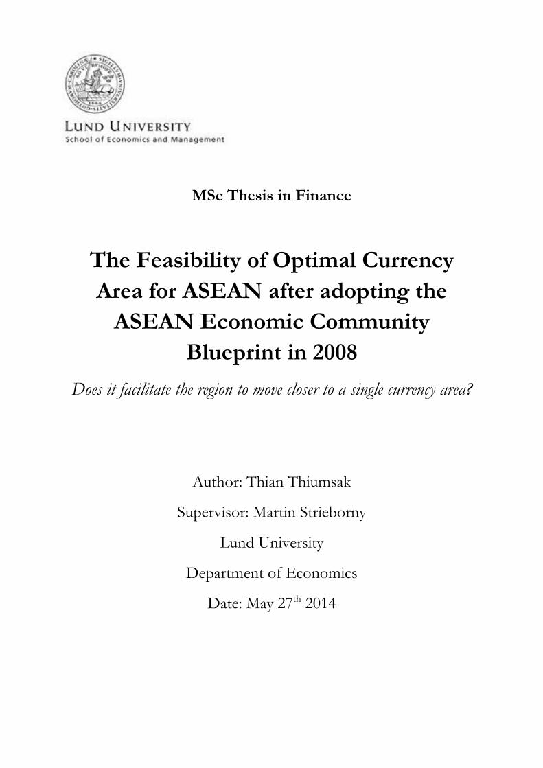
Based on the estimation results, time series plots of the conditional correlations for each
country pairs of the two variables can be created to investigate their evolution before and
after the implementation of integration policy in 2008. Figure 1 and 2 depict the dynamic of
all the correlations derived from the model. Given the average value of conditional
correlations shown in Table 12 and 13 and evidence of a structural break after the
implementation of the integration policy in 2008, it is not surprising that these conditional
correlation decrease over time, with the apparent change being between Thailand-Philippines
and Indonesia-Philippines for industrial production index growth and Philippines-Singapore
and Malaysia-Singapore for change in nominal interest rate.
A decrease in conditional correlation of most country pairs of industrial production index
growth rate and change in short-term interest rate after the implementation of integration
policy in 2008 indicates that the whole region diverges away from OCA and Maastricht
criteria and that the feasibility of OCA is decreased.
As discussed in Mundell (1961), individual monetary policy is used to adjust to shocks which
is specific to each country (i.e. asymmetric shocks). Therefore, the cost of adopting a
common currency is the inability for a country to use monetary policy to adjust to
asymmetric shocks. Following this logic, a higher asymmetric shocks increase the
opportunity cost of using a common currency.
To illustrate this theoretical framework, the explanation of De Grauwe (1992) of how
asymmetric monetary system (i.e. one member country take a leadership role in setting
policy) and asymmetric shock can cause problem to a region that pursuit single currency area.
Assuming that ASEAN adopts single currency and Singapore is allowed to be important in
determining the overall monetary stance for the region (just like Germany is for European
Union). Because of asymmetry of shock, if a specific macroeconomic shock hits the region,
some countries will encounter a contraction in GDP growth rate and some countries
(including Singapore for example) will experience an increase GDP growth rate. Since the
center country (Singapore) does not change its monetary policy stance as it benefits from the
shock, the rest of the countries which response negatively to shock can be in a deeper
recession as they lose individual monetary policy to adjust to shock.
Since conditional correlation of industrial production index growth rate measures to what
extent the two countries response differently to shocks (i.e. asymmetric shocks), a lower
correlation of the variable for most of the country pairs suggest higher asymmetric of shocks
31
for ASEAN. Applying the theoretical framework above to the result of this paper, due to
higher asymmetry of shock, there will be more countries response differently to the shock
from Singapore and the region’s GDP contraction will be even worsen than if asymmetry of
shock is lower.
As discussed in Maastricht criteria, the conditional correlation of short-term interest rate
measures monetary policy coordination, which is important for successful functioning of
OCA. A decline correlation of the variable for most of the country pair indicates lesser policy
synchronicity among country members and may interrupt functioning of OCA when the
region adopts it.
Hence, a decline in the conditional correlation of most country pairs of both variables after
the implementation of integration policy in 2008 demonstrates that the feasibility of OCA for
the region is worsened.
The results of this paper that higher economic integration due to integration policy causes
divergence in business cycle is in line with Krugman (1993) which, by using evidence from
North America, argues that increased economic integration does not guarantee economic
convergence but rather increase the possibility of asymmetric shocks as country members
become more locally specialized from the integration. A recent paper regarding the issue by
Imbs (2004) also confirm that specialization in the industry structure is negatively correlated
with business cycle synchronization. The research uses US data and is carried out by
employing system of simultaneous equations. Nevertheless, there is only weak evidence that
trade-induced specialization is negatively correlated with output comovement.
7. Conclusion
This paper investigates the feasibility of OCA for ASEAN after the implementation of
ASEAN Economic Community Blueprint (i.e. integration policy) in 2008. Dynamic
Conditional Correlation (DCC) model with and without a structural break is used to identify
whether the policy implemented facilitates the region to move closer to a single currency
area. Industrial production index growth rate and change in short-term interest rate for
ASEAN founders (Indonesia, Malaysia, Philippines, Singapore, and Thailand) are selected as
a proxy for OCA and Maastricht criteria respectively, which are cited as significant factors
for successful functioning of OCA.
32
In order to identify whether the integration policy implemented enables the region to
converge to a single currency area, three formal testing procedures is carried out. First,
average value of conditional correlations for each country pairs of the two variables before
and after the implementation of integration policy in 2008 is estimated using the DCC model
without a structural break. Second, the DCC model with a structural break for each country
pairs of the two variables is estimated and the graph is plotted accordingly. Third, the
likelihood ratio test statistic is computed using the value of log likelihood function from the
DCC model with and without a break. The results of three formal testing procedures indicate
that there is a structural break of conditional correlation of country pairs of the two variables
after the implementation of integration policy in 2008 and that most of the conditional
correlations decrease over time.
A decrease in conditional correlation of most country pairs of the two variables after the
implementation of integration policy in 2008 indicates that the whole region diverges away
from OCA and Maastricht criteria respectively and that the feasibility of OCA is decreased.
The result of this paper that higher economic integration due to integration policy causes
divergence in business cycle is in line with Krugman (1993) and Imbs (2004) which argues
that increased economic integration does not guarantee economic convergence but rather
increases the likelihood of asymmetric shocks (i.e. divergence in business cycle) as industry
of country members become more specialized.
In the case of ASEAN, as discussed in integration indicator and analysis section, there is an
evidence of higher economic integration after the implementation of integration policy in
2008, indicating by higher intra-regional trade, investment, and labor mobility. However, the
conditional correlation analysis used in this paper is unable to identify whether economic
integration actually causes specialization in the industry (integration-induced specialization)
to decrease business cycle synchronization, which is evidence in this paper. It only
demonstrates the development of the condition correlation of business cycle over time and,
hence, a progress of the feasibility of OCA for ASEAN. Therefore, for higher effectiveness
of future integration policy formulation, a further formal quantitative analysis needed to be
carried out in order to precisely identify that higher economic integration causes higher
specialization in the industry and, hence, more divergence in business cycle.
33
8. References
Adams, P. D. (2005). Optimal Currency Areas: Theory and Evidence for an African Single
Currency. University of Manchester.
Artis, M. J. (1991). One market, one money: An evaluation of the potential benefits and costs
of forming an economic and monetary union. Open economies review, 2(3), 315-321.
Artis, M. J. and Zhang, W. (2001) Core and Periphery in EMU: A Cluster Analysis.
Economic Issues 6(2): 39-60.
Bacha, O. I. (2008). A common currency area for ASEAN? Issues and feasibility. Applied
Economics, 40(4), 515-529.
Barro and Gordon (1983) A Positive Theory of Monetary Policy in a Natural Rate Model.
The Journal of Political Economy 91 (4): 589-610.
Bayoumi, T., & Eichengreen, B. (1997). Ever closer to heaven? An optimum-currency-area
index for European countries. European economic review, 41(3), 761-770.
Bayoumi, Tamim and Eichengreen, Barry (1994) One Money or Many? Analysing the
Prospects For Monetary Unification in Various Parts of the World. Princeton Studies in
International Finance No. 76 September 1994.
Bayoumi, T., Eichengreen, B., & Mauro, P. (2000). On regional monetary arrangements for
ASEAN. Journal of the Japanese and International Economies, 14(2), 121-148.
Bayoumi, T., & Mauro, P. (2001). The suitability of ASEAN for a regional currency
arrangement. The World Economy, 24(7), 933-954.
Blanchard, Olivier and Quah, Danny (1989) The Dynamic Effects of Aggregate Demand and
Supply Disturbances. American Economic Review 79: 655-673.
Blanchard, O., & Perotti, R. (2002). An empirical characterization of the dynamic effects of
changes in government spending and taxes on output. the Quarterly Journal of economics,
117(4), 1329-1368.
Boreiko, D. (2003). EMU and accession countries: Fuzzy cluster analysis of membership.
International Journal of Finance & Economics, 8(4), 309-325.
Bunyaratavej, K., & Hahn, E. D. (2003). Convergence and its implications for a common
currency in ASEAN. ASEAN Economic Bulletin, 20(1), 49-59.
De Grauwe, Paul (2000). Economics of Monetary Union (4th Edition). Oxford: Oxford
University Press.
Dennis, D. J., & Yusof, Z. A. (2003). Developing Indicators of ASEAN Integration: A
Preliminary Survey for a Roadmap. Regional Economic Policy Support Facility.
34
Engle, R. (2002). Dynamic conditional correlation: A simple class of multivariate generalized
autoregressive conditional heteroskedasticity models. Journal of Business & Economic
Statistics, 20(3), 339-350.
Engle, R. F., & Sheppard, K. (2001). Theoretical and empirical properties of dynamic
conditional correlation multivariate GARCH (No. w8554). National Bureau of Economic
Research.
Enders, Walter and Hurn, Stan (1994) Theory and Tests of Generalised Purchasing Power
Parity: Common Trends and Real Exchange Rates in the Pacific Rim. Review of International
Economics 2(2): 179-190.
Frankel, Jeffrey A. and Rose, Andrew K. (1997) ‘The Endogeneity of Optimum Currency
Area Criteria’ The Economic Journal 108(449): 1009-1025.
Frenkel, J., & Goldstein, M. (1987). A guide to target zones. Staff Papers, International
Monetary Fund, 33, 633-73.
Friedman, M. (1953). The case for flexible exchange rates. In Essays in Positive Economics,
M. Friedman (ed.), (University of Chicago Press), 157-203.
Friedman, M. (1968). The Role of Monetary Policy. A.E.R. 58 (March): 1–17.
Guerrero, R. B. (2008). Regional integration: the ASEAN vision in 2020. IFC Bulletin, 32,
52-58.
Imbs, J. (2004). Trade, finance, specialization, and synchronization. Review of Economics
and Statistics, 86(3), 723-734.
Kawai, M. (1987). Optimum currency areas. The New Palgrave: A Dictionary of Economics,
London: Macmillan Press, Ltd, 740-743.
Kenen, Peter B. (1969). The Theory of Optimal Currency Areas: An Eclectic View, pp 41-60
in Mundell, Robert A. and Swoboda, Alexander K.
Krugman, Paul (1993) Lessons of Massachusetts for EMU. pp241-261 in Giavazzi and
Torres eds. The Transition to Economic and Monetary Union in Europe, New York:
Cambridge University Press.
Lee, J. (2006). The comovement between output and prices: Evidence from a dynamic
conditional correlation GARCH model. Economics Letters, 91(1), 110-116.
Lee, J. (2006). The comovement between output and prices: Evidence from a dynamic
conditional correlation GARCH model. Economics Letters, 91(1), 110-116.
Li, X. M., & Zou, L. P. (2008). How do policy and information shocks impact co-movements
of China’s T-bond and stock markets? Journal of Banking & Finance, 32(3), 347-359.
35
Lucas Jr, R. E. (1972). Expectations and the Neutrality of Money. Journal of economic
theory, 4(2), 103-124.
McKinnon, R. I. (1963). Optimum currency areas. The American Economic Review, 717-
725.
Meade, J. E. (1955). The case for variable exchange rates. Three Banks Review, 27(3), 3-27.
Mkenda, B.K. (2001) Is East Africa an Optimum Currency Area?. Goteburg University
Department of Economics Working Paper No. 41 April 2000.
Mundell, R. A. (1961). A theory of optimum currency areas. &, 51, 657-65.
Ngo, K. P. (2013). Benefits, Costs, and Feasibility of a Monetary Union for the Association
of Southeast Asian Nations (ASEAN). Michigan Journal of Business, 6(1).
Rose, A.K. (2000) One Money, One Market: The Effect of Common Currencies on Trade.
Economic Policy April: 9-45.
Vaubel, R. (1976). Real exchange-rate changes in the European Community: The empirical
evidence and its implications for European currency unification. Weltwirtschaftliches Archiv,
112(3), 429-470.
Vaubel, R. (1978). Strategies for currency unification: the economics of currency competition
and the case for a European parallel currency (Vol. 156). Mohr.
Vu, T. K. (2008). Examining the Possibility of Introducing a Common Currency for
ASEAN─ An empirical analysis of symmetry of shocks.
36
9. Appendices
Figure 1: Conditional Correlations for each country pairs of industrial production index
growth rate
Thailand vs. Indonesia
-0,8
-0,6
-0,4
-0,2
0
0,2
0,4
0,6
0,8
1
Jan-
01
Aug
-01
Mar
-02
Oct
-02
May
-03
Dec
-03
Jul-0
4
Feb-
05
Sep-
05
Apr
-06
Nov
-06
Jun-
07
Jan-
08
Aug
-08
Mar
-09
Oct
-09
May
-10
Dec
-10
Jul-1
1
Feb-
12
Sep-
12
Apr
-13
Nov
-13
-0,6
-0,4
-0,2
0
0,2
0,4
0,6
0,8
1
Jan-
01
Aug
-01
Mar
-02
Oct
-02
May
-03
Dec
-03
Jul-
04
Feb-
05
Sep-
05
Apr
-06
Nov
-06
Jun-
07
Jan-
08
Aug
-08
Mar
-09
Oct
-09
May
-10
Dec
-10
Jul-
11
Feb-
12
Sep-
12
Apr
-13
Nov
-13
-0,6
-0,4
-0,2
0
0,2
0,4
0,6
0,8
1
1,2
Jan-
01
Aug
-01
Mar
-02
Oct
-02
May
-03
Dec
-03
Jul-
04
Feb-
05
Sep-
05
Apr
-06
Nov
-06
Jun-
07
Jan-
08
Aug
-08
Mar
-09
Oct
-09
May
-10
Dec
-10
Jul-
11
Feb-
12
Sep-
12
Apr
-13
Nov
-13
Thailand vs. Philippines
Thailand vs. Malaysia
37
-0,6
-0,4
-0,2
0
0,2
0,4
0,6
0,8
1
Jan-
01
Aug
-01
Mar
-02
Oct
-02
May
-03
Dec
-03
Jul-
04
Feb-
05
Sep-
05
Apr
-06
Nov
-06
Jun-
07
Jan-
08
Aug
-08
Mar
-09
Oct
-09
May
-10
Dec
-10
Jul-
11
Feb-
12
Sep-
12
Apr
-13
Nov
-13
-1
-0,8
-0,6
-0,4
-0,2
0
0,2
0,4
0,6
0,8
1
Jan-
01
Aug
-01
Mar
-02
Oct
-02
May
-03
Dec
-03
Jul-
04
Feb-
05
Sep-
05
Apr
-06
Nov
-06
Jun-
07
Jan-
08
Aug
-08
Mar
-09
Oct
-09
May
-10
Dec
-10
Jul-
11
Feb-
12
Sep-
12
Apr
-13
Nov
-13
-1
-0,8
-0,6
-0,4
-0,2
0
0,2
0,4
0,6
0,8
Jan-
01
Oct
-01
Jul-
02
Apr
-03
Jan-
04
Oct
-04
Jul-
05
Apr
-06
Jan-
07
Oct
-07
Jul-
08
Apr
-09
Jan-
10
Oct
-10
Jul-
11
Apr
-12
Jan-
13
Oct
-13
Thailand vs. Singapore
Indonesia vs. Philippines
Indonesia vs. Malaysia
38
-1
-0,8
-0,6
-0,4
-0,2
0
0,2
0,4
0,6
0,8
Jan-
01
Aug
-01
Mar
-02
Oct
-02
May
-03
Dec
-03
Jul-
04
Feb-
05
Sep-
05
Apr
-06
Nov
-06
Jun-
07
Jan-
08
Aug
-08
Mar
-09
Oct
-09
May
-10
Dec
-10
Jul-
11
Feb-
12
Sep-
12
Apr
-13
Nov
-13
-0,8
-0,6
-0,4
-0,2
0
0,2
0,4
0,6
0,8
1
Jan-
01
Aug
-01
Mar
-02
Oct
-02
May
-03
Dec
-03
Jul-
04
Feb-
05
Sep-
05
Apr
-06
Nov
-06
Jun-
07
Jan-
08
Aug
-08
Mar
-09
Oct
-09
May
-10
Dec
-10
Jul-
11
Feb-
12
Sep-
12
Apr
-13
Nov
-13
-0,6
-0,4
-0,2
0
0,2
0,4
0,6
0,8
1
Jan-
01
Aug
-01
Mar
-02
Oct
-02
May
-03
Dec
-03
Jul-
04
Feb-
05
Sep-
05
Apr
-06
Nov
-06
Jun-
07
Jan-
08
Aug
-08
Mar
-09
Oct
-09
May
-10
Dec
-10
Jul-
11
Feb-
12
Sep-
12
Apr
-13
Nov
-13
Indonesia vs. Singapore
Philippines vs. Malaysia
Philippines vs. Singapore
39
Figure 2: Conditional Correlations for each country pairs of change in short-term interest rate
-1
-0,8
-0,6
-0,4
-0,2
0
0,2
0,4
0,6
0,8
1
Jan-
01
Aug
-01
Mar
-02
Oct
-02
May
-03
Dec
-03
Jul-0
4
Feb-
05
Sep-
05
Apr
-06
Nov
-06
Jun-
07
Jan-
08
Aug
-08
Mar
-09
Oct
-09
May
-10
Dec
-10
Jul-1
1
Feb-
12
Sep-
12
Apr
-13
Nov
-13
-1
-0,8
-0,6
-0,4
-0,2
0
0,2
0,4
0,6
0,8
1
1,2
Jan
-01
Au
g-0
1
Ma
r-02
Oct
-02
Ma
y-0
3
De
c-03
Jul-
04
Feb
-05
Sep
-05
Ap
r-0
6
No
v-0
6
Jun
-07
Jan
-08
Au
g-0
8
Ma
r-09
Oct
-09
Ma
y-1
0
De
c-10
Jul-
11
Feb
-12
Sep
-12
Ap
r-1
3
No
v-1
3
-0,6
-0,4
-0,2
0
0,2
0,4
0,6
0,8
1
Jan-
01
Aug
-01
Mar
-02
Oct
-02
May
-03
Dec
-03
Jul-
04
Feb-
05
Sep-
05
Apr
-06
Nov
-06
Jun-
07
Jan-
08
Aug
-08
Mar
-09
Oct
-09
May
-10
Dec
-10
Jul-
11
Feb-
12
Sep-
12
Apr
-13
Nov
-13
Malaysia vs. Singapore
Thailand vs. Indonesia
Thailand vs. Philippines
40
-1
-0,5
0
0,5
1
1,5
Jan-
01
Sep-
01
May
-02
Jan-
03
Sep-
03
May
-04
Jan-
05
Sep-
05
May
-06
Jan-
07
Sep-
07
May
-08
Jan-
09
Sep-
09
May
-10
Jan-
11
Sep-
11
May
-12
Jan-
13
Sep-
13
-1,5
-1
-0,5
0
0,5
1
1,5
Jan-
01
Sep-
01
May
-02
Jan-
03
Sep-
03
May
-04
Jan-
05
Sep-
05
May
-06
Jan-
07
Sep-
07
May
-08
Jan-
09
Sep-
09
May
-10
Jan-
11
Sep-
11
May
-12
Jan-
13
Sep-
13
-1
-0,8
-0,6
-0,4
-0,2
0
0,2
0,4
0,6
0,8
1
Jan-
01
Sep-
01
May
-02
Jan-
03
Sep-
03
May
-04
Jan-
05
Sep-
05
May
-06
Jan-
07
Sep-
07
May
-08
Jan-
09
Sep-
09
May
-10
Jan-
11
Sep-
11
May
-12
Jan-
13
Sep-
13
Thailand vs. Malaysia
Thailand vs. Singapore
Indonesia vs. Philippines
41
-1,5
-1
-0,5
0
0,5
1
1,5
Jan-
01
Sep-
01
May
-02
Jan-
03
Sep-
03
May
-04
Jan-
05
Sep-
05
May
-06
Jan-
07
Sep-
07
May
-08
Jan-
09
Sep-
09
May
-10
Jan-
11
Sep-
11
May
-12
Jan-
13
Sep-
13
-1
-0,8
-0,6
-0,4
-0,2
0
0,2
0,4
0,6
0,8
1
Jan-
01
Sep-
01
May
-02
Jan-
03
Sep-
03
May
-04
Jan-
05
Sep-
05
May
-06
Jan-
07
Sep-
07
May
-08
Jan-
09
Sep-
09
May
-10
Jan-
11
Sep-
11
May
-12
Jan-
13
Sep-
13
-1
-0,5
0
0,5
1
1,5
Jan-
01
Sep-
01
May
-02
Jan-
03
Sep-
03
May
-04
Jan-
05
Sep-
05
May
-06
Jan-
07
Sep-
07
May
-08
Jan-
09
Sep-
09
May
-10
Jan-
11
Sep-
11
May
-12
Jan-
13
Sep-
13
Indonesia vs. Malaysia
Indonesia vs. Singapore
Philippines vs. Malaysia
42
-1
-0,5
0
0,5
1
1,5
Jan-
01
Sep-
01
May
-02
Jan-
03
Sep-
03
May
-04
Jan-
05
Sep-
05
May
-06
Jan-
07
Sep-
07
May
-08
Jan-
09
Sep-
09
May
-10
Jan-
11
Sep-
11
May
-12
Jan-
13
Sep-
13
-1
-0,8
-0,6
-0,4
-0,2
0
0,2
0,4
0,6
0,8
1
1,2
Jan
-01
Jul-
01
Jan
-02
Jul-
02
Jan
-03
Jul-
03
Jan
-04
Jul-
04
Jan
-05
Jul-
05
Jan
-06
Jul-
06
Jan
-07
Jul-
07
Jan
-08
Jul-
08
Jan
-09
Jul-
09
Jan
-10
Jul-
10
Jan
-11
Jul-
11
Jan
-12
Jul-
12
Jan
-13
Jul-
13
Philippines vs. Singapore
Malaysia vs. Singapore