The Fermionic Observable in the Ising Model and the Inverse Kac–Ward Operator

Ann. Henri Poincare Online Firstc© 2013 Springer BaselDOI 10.1007/s00023-013-0295-z Annales Henri Poincare

The Fermionic Observable in the Ising Modeland the Inverse Kac–Ward Operator

Marcin Lis

Abstract. We show that the critical Kac–Ward operator on isoradialgraphs acts in a certain sense as the operator of s-holomorphicity, and weidentify the fermionic observable for the spin Ising model as the inverseof this operator. This result is partially a consequence of a more generalobservation that the inverse Kac–Ward operator on any planar graph isgiven by what we call a fermionic generating function. We also present ageneral picture of the non-backtracking walk representation of the criticaland supercritical inverse Kac–Ward operators on isoradial graphs.

Introduction

The discrete fermionic observable for the FK-Ising model on the square latticewas introduced by Smirnov [22] (although, as mentioned in [8], similar objectsappeared in earlier works). He proved in [23] that its scaling limit at critical-ity is given by the solution to a Riemann–Hilbert boundary value problem,and therefore is conformally covariant. A generalization of this result to Isingmodels defined on a large class of isoradial graphs was obtained by Chelkakand Smirnov [8], yielding also universality of the scaling limit.

Since then, several different types of observables have been proposed forboth the random cluster and classical spin Ising model. They were used toprove conformal invariance of important quantities in these models. The scal-ing limit of the energy density of the critical spin Ising model on the squarelattice was computed by Hongler and Smirnov [14]. Existence and conformalinvariance of the scaling limits of the magnetization and multi-point spin corre-lations were established by Chelkak et al. [6]. The observable also proved usefulin the off-critical regime and was employed by Beffara and Duminil-Copin [2]to give a new proof of criticality of the self-dual point and to calculate the cor-relation length in the Ising model on the square lattice. In a more recent workof Hongler et al. [13], the fermionic observables were identified as correlation

M. Lis Ann. Henri Poincare

functions of fermion operators in the transfer matrix formalism for the samemodel. One also has to mention the relation between the fermionic observableand the inverse Kasteleyn operator which was pointed out by Dubedat [11].

In this paper, we establish a direct connection between the fermionicobservable for the spin Ising model and the inverse Kac–Ward operator. Themethod of Kac and Ward [15] is a way of expressing the square of the par-tition function of the Ising model on a planar graph as the determinant ofthe Kac–Ward operator. It was proposed as a combinatorial alternative to thepurely algebraic approach developed by Onsager and Kaufman [18,21]. TheKac–Ward method and the Kac–Ward operator itself have recently becomean object of revived interest. A thorough treatment of this approach with afocus on the combinatorics of configurations of loops was presented by Kager,Meester and the author in [16]. The method was used there to rederive the crit-ical point of the Ising model on the square lattice and to obtain new expressionsfor the free energy density and spin correlation functions in terms of signedloops and non-backtracking walks in the graph. The same formulas for finitegraphs were independently obtained by Helmuth [12], where the Kac–Wardmethod was put into a more general combinatorial context of heaps of pieces.Also in [12], the spinor fermionic observable from [6,7] was explicitly identi-fied in terms of non-backtracking walks, though without addressing the issuesof convergence of the expansions. In [20] the author, following the ideas con-tained in [16], obtained bounds on the spectral radius and operator norm ofthe Kac–Ward transition matrix on a general graph and proved criticality ofthe self-dual Z-invariant Ising model introduced by Baxter [1]. Other relevantexamples are the extension of the Kac–Ward method to graphs of higher genusintroduced by Cimasoni [9] and the computation of the critical temperatureof the Ising model on doubly periodic planar graphs performed by Cimasoniand Duminil-Copin [10].

This paper consists of three sections. In Sect. 1 we define the Kac–Wardoperator on a general graph in the plane. We then describe properties of thecomplex weights induced by this operator on the non-backtracking walks inthe graph. In the end, we use loop expansions of the even subgraph generat-ing function from [16] to express the inverse Kac–Ward operator on a finitegraph in terms of a weighted sum over a certain family of subgraphs. We callthe resulting formula the fermionic generating function since it bears a strongresemblance to the definitions of the spin fermionic observables from [8,13,14].In Sect. 2 we work on isoradial graphs. First, we consider the Kac–Ward oper-ator corresponding to the critical Ising model and we show that it can bethought of as the operator of s-holomorphicity. Subsequently, using boundsfrom [20], we show that in finite volume the inverted critical Kac–Ward oper-ator admits a representation in terms of non-backtracking walks, whereas acontinuous inverse in infinite volume does not exist. We also consider thesupercritical inverse operators. They too are expressed in terms of walks (bothon finite and infinite graphs), and moreover the associated Green’s functiondecays exponentially fast with the distance between two edges. In particular,the supercritical operator on the full isoradial graph has a continuous inverse.

Fermionic Observable and Inverse Kac–Ward Operator

As a remark, we would like to point out that our observations seem tofit into a more general picture of two-dimensional discrete physical modelssatisfying the following three conditions:

(i) the partition function of the model is equal to the square root of thedeterminant of some operator,

(ii) an important observable in the model is given by the inverse of thisoperator,

(iii) the critical values of parameters of the model coincide with the valuesof parameters which make this operator into some (massless) discretedifferential operator.

Our results show that the Ising model on isoradial graphs satisfies this clas-sification with the distinguished operator being the Kac–Ward operator, theobservable being the fermionic observable, and the discrete differential operatorbeing the s-holomorphic operator. Another example is the discrete Gaussianfree field, where the partition function is equal to the square root of the deter-minant of the discrete Laplacian, and the two-point spin correlation functionsare given by the inverse of the Laplacian. Moreover, the general picture ofthe non-backtracking walk representation of the inverse Kac–Ward operatorpresented in Sect. 2 matches the one of the random walk representation of theinverse Laplacian [5]. Also the dimer model [17], which is known to be closelyrelated to the Ising model, fits this pattern. The square of the partition sum ofthis model is equal to the absolute value of the determinant of the Kasteleynoperator, which acts as the discrete Dirac operator (see e.g. [19]). In addition,the observable of main interest in the work of Kenyon [19] is the couplingfunction defined as the inverse of the Kasteleyn operator.

1. The Kac–Ward Operator and Graph Generating Functions

We will consider graphs embedded in the complex plane. To simplify our nota-tion, we will identify graphs with their edge sets. By an (undirected) edge wemean an unordered pair of distinct complex numbers {z, w}, which we willidentify with the closed straight line segment in the complex plane connectingz and w. We say that z and w are the endpoints of {z, w}. A collection ofedges G is called a graph if any two edges in G share at most one point, whichis either an endpoint of both of them, or is not an endpoint of any edge in G.In the latter case we say that the two edges cross each other. A complexnumber z is called a vertex in G if it is an endpoint of some edge in G.

Although a graph G is undirected, we will mainly work with the directededges of G, i.e. the ordered pairs of complex numbers (z, w) for which {z, w} ∈G. We write �G for the set of all directed edges of G. We will always denotea directed edge by a letter with an arrow over it, whereas the undirectedcounterpart will be obtained by dropping the arrow from the notation, i.e. if�e = (z, w), then e = {z, w}. For a directed edge �e = (z, w), we define its tailt(�e) = z and its head h(�e) = w, and we write −�e for the inverted edge (w, z).


1.1. The Kac–Ward Operator

From now on, we assume that G is a fixed (possibly infinite) graph with finitemaximal degree, and x = (xe)e∈G is a system of positive edge weights satisfying‖x‖∞ = supe∈G xe < ∞. For two directed edges �e and �g, let

∠(�e,�g) = Arg(

h(�g) − t(�g)h(�e) − t(�e)

)∈ (−π, π] (1.1)

be the turning angle from �e to �g. The (Kac–Ward) transition matrix is givenby

Λ�e,�g =

{xee

i2 ∠(�e,�g) if h(�e) = t(�g) and �g �= −�e;

0 otherwise.(1.2)

The Kac–Ward operator is an automorphism of the complex vector space C�G

defined via matrix multiplication by the matrix

T = Id − Λ,

where Id is the identity matrix. Note that this is well defined since T hasat most Δ nonzero entries in each row, where Δ is the maximal degree of G.Moreover, since the weight system is bounded, T is continuous (bounded) whentreated as an operator on �2(�G). It is known, that if G is finite and no two edgesin G cross each other, then the determinant of T is strictly larger than one(see Theorem 1.3). In particular, in this case T is an isomorphism.

1.2. Weighted Non-Backtracking Walks

A (non-backtracking) walk ω of length |ω| = n in G is a sequence of directededges ω = (�e0, �e1, . . . , �en) ∈ �Gn+1, such that h(�ei) = t(�ei+1) and �ei+1 �= −�ei

for i = 0, . . . , n−1. Note that |ω| counts the number of steps ω makes betweenedges, rather than the number of edges it visits. A walk ω is closed if �e0 = �en

and |ω| > 0. We say that ω goes through a directed edge �e (undirected edge e) if�ei = �e (ei = e) for some i ∈ {0, . . . , n−1}. Note that ω does not necessarily gothrough �en, and in particular walks of length zero do not go through any edge.By E(ω) we denote the edge set of ω, i.e. the set of undirected edges that thewalk ω goes through. A walk is called a path if it goes through every undirectededge at most once. By −ω we mean the reversed walk (−�en,−�en−1, . . . ,−�e0).

The (signed) weight of a walk ω = (�e0, �e1, . . . , �en) is given by

w(ω) = ei2 α(ω)

n−1∏i=0

xei, where α(ω) =

n−1∑i=0

∠(�ei, �ei+1) (1.3)

is the total turning angle of ω. Note that with this definition of the signedweight, the last edge of ω is not counted in terms of edge weights, but doescontribute to the total winding angle of ω. In particular, w(ω) is a monomial inthe variables xe, e ∈ E(ω). If |ω| = 0, then we put α(ω) = 0 and w(ω) = 1. Thefundamental feature of the signed weight is that it factorizes over the steps


that a path makes, where the step weight is given by the transition matrix(1.2), i.e.

w(ω) =n−1∏i=0

Λ�ei,�ei+1 . (1.4)

Given two directed edges �e and �g, we write W(�e,�g) for the collection ofall walks in G which start at �e and end at �g. Since the complex argumentsatisfies the logarithmic identity Arg(z/w) = Arg(z) − Arg(w) (mod 2π), weconclude that

w(ω) ∈ ei2 ∠(�e,�g)R for ω ∈ W(�e,�g). (1.5)

On the other hand, since walks are non-backtracking and Arg(1/z) = −Arg(z)for z /∈ (−∞, 0], it follows that α(ω) = −α(−ω). Combining these two facts,we obtain that

w(ω) =

{−w(−ω) if ω ∈ W(�e,−�e);

w(−ω) if ω ∈ W(�e,�e).(1.6)

The first identity in (1.6) implies cancellations of weights of walks which gothrough certain edges in both directions. The most basic consequence of thisproperty is the following lemma:

Lemma 1.1. For any �e ∈ �G, ∑ω∈W(�e,−�e)

w(ω) = 0.

Proof. If W(�e,−�e) is empty, then the above statement is trivially true. Other-wise, if ω ∈ W(�e,−�e), then −ω ∈ W(�e,−�e), w(ω) = −w(−ω), and −(−ω) = ω.Hence, we have cancellation of all terms in the series. �

This observation and others which naturally follow from property (1.6)(see Lemmas 3.1 and 3.2 in Sect. 3) will be important in the computation ofthe inverse of the Kac–Ward operator.

Note that the above sum is in general an infinite power series in thevariables xe. To be rigorous when dealing with power series, we will alwaysassume, unless stated otherwise, that ‖x‖∞ is sufficiently small for the seriesto be absolutely convergent. In all of the cases, it will be enough to take‖x‖∞ < 1/(Δ − 1).

1.3. Crossings in Graphs and Walks

As mentioned before, edges of a graph can cross each other. For a finitegraph H, let C(H) be the number of edge crossings in H, i.e. the numberof unordered pairs of edges in H which cross each other.

A similar notion of a crossing can be assigned to closed walks. One canthink of a closed walk ω = (�e0, . . . , �en) as a closed continuous curve in thecomplex plane with the time parametrization given by

ω(s) = t(�e�s�) + (s − �s�)(h(�e�s�) − t(�e�s�)) for s ∈ R/nZ.


With this definition, we say that (s1, s2) ∈ (R/|ω1|Z) × (R/|ω2|Z) is a cross-ing at z between two closed walks ω1 and ω2, if z = ω1(s1) = ω2(s2),and for any small open neighborhood U1 × U2 of (s1, s2), there is a smallball B around z, such that ω1(U1) intersects both connected components ofB\ω2(U2). Note that in our setting, the only possible crossings between closedwalks can occur at the vertices of G, or at the points of crossings of edgesof G. We write C(ω1, ω2) for the number of crossings between ω1 and ω2, andC(ω) = C(ω, ω)/2 for the number of self-crossings of ω.

We say that two walks are edge disjoint if their edge sets are disjoint. Fortopological reasons, if ω1 and ω2 are edge-disjoint closed paths, then C(ω1, ω2)is even. Moreover, there is an intrinsic connection between the total turningangle of a closed path and the number of its self-crossings:

Theorem 1.2 (Whitney [24]). For any closed path ω,

−ei2 α(ω) = (−1)C(ω).

1.4. Generating Functions of Even Subgraphs

We call a graph H even if all its vertices have even degree. Equivalently, afinite graph H is even if and only if it is a union of edge sets of some collectionof edge-disjoint closed paths. The generating function of even subgraphs of afinite graph G, as defined in [16], is given by

Z =∑H⊂G

H even

(−1)C(H)∏e∈H

xe. (1.7)

The empty set is also even and we assume that its contribution to Z equalsone. If G has no edge crossings, then Z counts all even subgraphs with positivesign, and in particular is bigger than one. If additionally ‖x‖∞ ≤ 1, then by thehigh-temperature expansion, Z is proportional to the partition function of theIsing model on G with free boundary conditions and with appropriate couplingconstants (see e.g. [16]). However, it will be crucial for the computation of theinverse Kac–Ward operator to allow graphs with crossings, and therefore wewill need the following result:

Theorem 1.3. [16]*Theorem 1.9

Z = exp

(−

∑ω closed

w(ω)2|ω|

)=

√detT ,

where the sum is over all closed walks in G.

The first equality of this theorem yields a direct connection between thegenerating function of even subgraphs and the signed non-backtracking walks.Note that the notation used here differs from the one in [16]. In particular,the signed weight from [16] is minus the signed weight defined in (1.3). Also,the corresponding exponential formula in [16] is written in terms of loops, i.e.equivalence classes of closed walks defining the same, up to a time parame-trization, closed curve in the plane. The signed weight of a loop is then definedas the sum of signed weights of closed walks in the equivalence class.


1.5. The Inverse Kac–Ward Operator

In this section we assume that G is finite and without edge crossings. If onewants to compute the inverse of the Kac–Ward operator, one can use the powerseries formula:

T−1�e,�g = (Id − Λ)−1

�e,�g =∞∑

n=0

Λn�e,�g =

∑ω∈W(�e,�g)

w(ω), (1.8)

which is valid for ‖x‖∞ small enough. The last sum is over all non-backtracking walks since the transition matrix Λ assigns zero weight to stepsbetween �e and −�e. It turns out that this sum can be expressed in terms of agenerating function of certain subgraphs of G (or rather its particular modifi-cation).

To this end, let m(�e) = (t(�e) + h(�e))/2 be the midpoint of �e. Given�e,�g ∈ �G, we define a modified graph

G�e,�g = (G\{e, g}) ∪ {{m(�e), h(�e)}, {t(�g),m(�g)}}which, instead of e and g, contains appropriate half-edges. The weight of{m(�e), h(�e)} is set to be xe, and in the case when �g �= −�e the weight of{t(�g),m(�g)} is one. We write E(�e,�g) for the collection of subgraphs H ⊂ G�e,�g

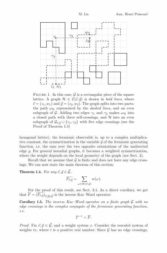
containing the half-edges {m(�e), h(�e)} and {t(�g),m(�g)}, and such that all ver-tices of G have even degree in H (see Fig. 1). Note that we do not requirethat m(�e) and m(�g) have even degree. It follows that E(�e,−�e) is empty, sincethere is no graph which has exactly one vertex with odd degree. Also notethat E(�e,�e) is in bijective correspondence with the set of even subgraphs of Gcontaining e.

Suppose that �g �= −�e and take H ∈ E(�e,�g). It follows that there is apath in H which starts at (m(�e), h(�e)) and ends at (t(�g),m(�g)). Let ωH bethe left-most such path, i.e. the path which always makes a step to the left-most edge which has not yet been visited in any direction. Note that H splitsinto ωH and an even subgraph of G (see Fig. 1). Since H also belongsto E(−�g,−�e) this notation may be ambiguous (the reversed left-most pathbecomes the right-most path), but we will always use it in the context of fixededges �e and �g.

For �e,�g ∈ �G, we define the fermionic generating function by

F�e,�g = δ�e,�g +1Z

∑H∈E(�e,�g)

e− i2 α(ωH)

∏h∈H

xh, (1.9)

where δ is the Kronecker delta. For �g = −�e, the above sum is empty and wetake it to be zero.

Note the resemblance between this definition and the definitions of fermi-onic observables from [8,13,14]. The important difference is that the fermi-onic generating function is a function of two directed edges and the fermionicobservable from the literature can be seen as a function of one directed andone undirected edge. Indeed, for regular lattices (the square, triangular and


Figure 1. In this case, G is a rectangular piece of the squarelattice. A graph H ∈ E(�e,�g) is drawn in bold lines, where�e = (z1, w1) and �g = (z2, w2). The graph splits into two parts:the path ωH represented by the dashed lines, and an evensubgraph of G. Adding two edges γ1 and γ2 makes ωH intoa closed path with three self-crossings, and H into an evensubgraph of G�e,�g ∪ {γ1, γ2} with five edge crossings (see theProof of Theorem 1.4)

hexagonal lattice), the fermionic observable is, up to a complex multiplica-tive constant, the symmetrization in the variable �g of the fermionic generatingfunction, i.e. the sum over the two opposite orientations of the undirectededge g. For general isoradial graphs, it becomes a weighted symmetrization,where the weight depends on the local geometry of the graph (see Sect. 2).

Recall that we assume that G is finite and does not have any edge cross-ings. We can now state the main theorem of this section:

Theorem 1.4. For any �e,�g ∈ �G,

F�e,�g =∑

ω∈W(�e,�g)

w(ω).

For the proof of this result, see Sect. 3.1. As a direct corollary, we getthat F = (F�e,�g)�e,�g∈�G is the inverse Kac–Ward operator:

Corollary 1.5. The inverse Kac–Ward operator on a finite graph G with noedge crossings is the complex conjugate of the fermionic generating function,i.e.

T−1 = F .

Proof. Fix �e,�g ∈ �G, and a weight system x. Consider the rescaled system ofweights tx, where t is a positive real number. Since G has no edge crossings,


Z is never zero by (1.7) and it follows from Theorem 1.3 that detT is alsonever zero. Hence, F�e,�g and T−1

�e,�g , treated as functions of the scaling factor t,are analytic on (0,∞). By uniqueness of the analytic continuation, it is enoughto prove the desired equality for t small, and this follows from Theorem 1.4and the power series expansion (1.8). �

Note that the fermionic generating function was defined only for finitegraphs. Theorem 1.4 and Corollary 1.5 give two interpretations of F whichdo not require finiteness of the underlying graph. We will discuss this issue inSect. 2.

2. The Kac–Ward Operator on Isoradial Graphs

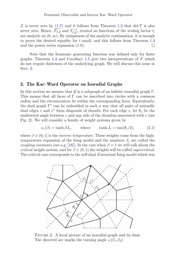
In this section we assume that G is a subgraph of an infinite isoradial graph Γ.This means that all faces of Γ can be inscribed into circles with a commonradius and the circumcenters lie within the corresponding faces. Equivalently,the dual graph Γ∗ can be embedded in such a way that all pairs of mutuallydual edges e and e∗ form diagonals of rhombi. For each edge e, let θe be theundirected angle between e and any side of the rhombus associated with e (seeFig. 2). We will consider a family of weight systems given by

xe(β) = tanh βJe, where tanh Je = tan(θe/2), (2.1)

where β ∈ (0, 1] is the inverse temperature. These weights come from the high-temperature expansion of the Ising model and the numbers Je are called thecoupling constants (see e.g. [16]). In the case when β = 1 we will talk about thecritical weight system, and for β ∈ (0, 1) the weights will be called supercritical.The critical case corresponds to the self-dual Z-invariant Ising model which was

Figure 2. A local picture of an isoradial graph and its dual.The directed arc marks the turning angle ∠(�e1, �e2)


introduced by Baxter [1] and has been extensively studied in the mathemat-ical literature. Chelkak and Smirnov proved in [8] that the critical fermionicobservable has a universal, conformally invariant scaling limit. Boutillier andde Tiliere [3,4] analysed the model using the dimer representation, and theauthor [20] proved that, after introducing the inverse temperature parameter,the model has a phase transition at β = 1 and nowhere else.

2.1. The Critical Kac–Ward Operator and s-Holomorphicity

In this section we assume that the weight system is critical. The notion ofs-holomorphicity (s stands for strong or spin) was introduced in [23] in thesetting of the square lattice and was later generalized in [8] to fit the context ofgeneral isoradial graphs. Our definition of s-holomorphicity will be equivalentto that in [8], up to multiplication of the function by some globally fixedcomplex constant.

Consider a vertex z in Γ and let z∗ be a vertex in Γ∗ corresponding toone of the faces of Γ incident to z. By e1 and e2, we denote the two edges lyingon the boundary of this face and having z as an endpoint (see Fig. 2). We saythat a complex function f defined on the edges of Γ is s-holomorphic at z iffor all such dual vertices z∗ and the corresponding edges e1 and e2,

Proj(f(e1); (z − z∗)− 12R) = Proj(f(e2); (z − z∗)− 1

2R),

where Proj(w; �) is the orthogonal projection of the complex number w ontothe line �. Note that the choice of the square root is immaterial in the def-inition above. The property of being s-holomorphic is a real linear prop-erty, i.e. addition of two functions and multiplication of a function by areal number preserve s-holomorphicity. It is also a stronger property thanthe usual discrete holomorphicity: if a function is s-holomorphic at z, thenthe same function considered as a function on the dual edges is discreteholomorphic at z, i.e. the discrete contour integral around the face correspond-ing to z vanishes. On the other hand, each discrete holomorphic function is, upto an additive constant, uniquely represented as a sum of two s-holomorphicfunctions, where one of them is multiplied by i. For proofs of these facts andother properties of s-holomorphic functions, see [8].

The Kac–Ward operator was defined in Sect. 1 as an automorphism ofthe complex vector space C

�G , but it can also be seen as an operator acting ona smaller real vector space. To be precise, to each directed edge �e we associatea line ��e in the complex plane defined by

��e = e− i2 ∠(�e)R, where ∠(�e) = Arg(h(�e) − t(�e)).

As before, we use the principal value of the complex argument. Note that ��e

and �−�e are orthogonal and they can be thought of as “a local coordinatesystem at e”. We will consider the direct product of the lines treated as one-dimensional real vector spaces, i.e. we put

L =∏�e∈�G

��e.


By the logarithmic property of the complex argument, T�e,�g defines by multi-plication a linear map from ��g to ��e. This means that the Kac–Ward operatorcan be seen as an automorphism of L. We define X to be CG treated as a realvector space and we consider an isomorphism between X and L given by

Sf(�e) = sin(θe/2)Proj(f(e); ��e) for f ∈ X .

If Γ is a regular lattice (the square, triangular or hexagonal lattice), thenall the angles θe are equal and S is proportional to the projection operatorwhich gives “local coordinates” at each edge. Note that the inverse of S is justa locally rescaled symmetrization operator, i.e.

S−1ϕ(e) = (sin(θe/2))−1(ϕ(�e) + ϕ(−�e)) for ϕ ∈ L.

We say that z is an interior vertex of G if the degrees of z in G and Γ arethe same. The set of edges emanating from a vertex z is denoted by Out(z) ={�e ∈ �G : t(�e) = z}, and In(z) = {�e ∈ �G : h(�e) = z} = −Out(z) are the edgespointing at z. The next result expresses the fact that the critical Kac–Wardoperator (composed with S) can be seen as the operator of s-holomorphicity:

Theorem 2.1. Let T be the critical Kac–Ward operator. A function f ∈ X iss-holomorphic at an interior vertex z if and only if

TSf(�e) = 0 for all �e ∈ In(z).

The proof of this theorem is given in Sect. 3.2.Consider the case where G is the full Γ and take f to be equal to one

everywhere. Of course, f is s-holomorphic at all vertices of Γ. It follows fromthe theorem above that TSf is equal to zero everywhere and hence the criticalKac–Ward operator for the full isoradial graph has a nontrivial kernel. Inparticular, it is not invertible on L and therefore also on C

�G .Let us go back to the case where G is a finite subgraph of Γ. From

Sect. 1.5, we know that the inverse Kac–Ward operator exists for allweight systems on G. As a consequence of Theorem 2.1, we can constructs-holomorphic functions by applying the inverse of TS to functions whichare zero almost everywhere. To this end, we define the standard basis of Lto be the set of functions {i�e}�e∈�G , where i�e(�g) = e− i

2 ∠(�e)δ�e,�g. It follows thatf�e = (TS)−1i−�e is s-holomorphic at all interior vertices of G which are not t(�e),and is not s-holomorphic at t(�e). We also have that

f�e(g) = S−1T−1i−�e(g)

∼ (sin(θg/2))−1(T−1�g,−�e + T−1

−�g,−�e)

∼ (cos(θg/2))−1(F�e,�g + F�e,−�g),

where ∼ means equality up to a multiplicative constant depending only on �e.We used here Corollary 1.5, the fact that xeT

−1�g,�e = xgT

−1−�e,−�g, and the definition

of the critical weight system. As mentioned before, the cosine term vanishesfrom this expression if Γ is a regular lattice. Recalling the definition of F ,one can see that f�e is proportional to the critical fermionic observable used in[8,13,14].


2.2. The Non-Backtracking Walk Representation

In this section we provide a representation of the inverse Kac–Ward operator interms of non-backtracking walks. Note that we already used this idea in (1.8),but only for weights which were sufficiently small in the supremum norm.It turns out that the walk expansions on isoradial graphs are valid for bothsupercritical and critical weight systems, though their behavior is different ineach of these cases.

We will use tools from [20] and hence we need a regularity condition on Γ,i.e. we will assume that there exist constants k and K such that

0 < k ≤ θe ≤ K < π for all e ∈ E(Γ). (2.2)

Geometrically, this means that the area of the underlying rhombi is uniformlybounded away from zero, or in other words the rhombi do not get arbitrarilythin.

For �e,�g ∈ �G, we define Wn(�e,�g) ⊂ W(�e,�g) to be the subcollection of allwalks of length n, and let d(�e,�g) be the distance between �e and �g, i.e. thelength of a shortest walk in W(�e,�g). All operators in the following statementare treated as operators on the Hilbert space �2(�G).

Theorem 2.2. If the weights are supercritical and G is a subgraph of Γ, or theweights are critical and G is a finite subgraph of Γ, then the inverse Kac–Wardoperator is continuous and is given by the matrix

T−1�e,�g =

∞∑n=d(�e,�g)

∑ω∈Wn(�e,�g)

w(ω).

Moreover, in the supercritical case, there exist constants C and ε < 1 such that∣∣∣∣∣∣∑

ω∈Wn(�e,�g)

w(ω)

∣∣∣∣∣∣ ≤ Cεn for all �e,�g and n.

Furthermore, C and ε depend only on β and on the isoradial graph Γ, and donot depend on the particular choice of G.

Finally, if G is the full Γ, then the critical Kac–Ward operator does nothave a continuous inverse.

Section 3.3 is devoted to the proof of this result. Note that this theo-rem and Corollary 1.5 provide a natural definition of the supercritical fermi-onic generating function on infinite isoradial graphs. Furthermore, the criticalfermionic observable on finite graphs also admits a representation in terms ofnon-backtracking walks.

We would like to mention that one could also consider Kac–Ward oper-ators with subcritical weights on the dual graph Γ∗, i.e. weights given byxe∗ = exp(−2βJe), where tanh Je = tan(θe/2) and β > 1. Since Γ∗ is alsoisoradial, the corresponding analysis would be similar due to the Kramers–Wannier duality of the planar Ising model (see [16,20]).

As mentioned in the introduction, the picture that Theorem 2.2 presentsmatches the one of the random walk representation of the inverse Laplacian [5]


on the square lattice. Indeed, the inverse of the Laplacian in finite volumeis given by the random walk Green’s function. Off criticality, i.e. when theLaplacian is massive, the Green’s function decays exponentially fast with thedistance between two vertices. As a result, the inverse of the massive operatorin the whole plane exists and is continuous. On the other hand, the full-planemassless Laplacian does not have a bounded inverse.

The crucial difference between these two representations seems to be thefact that the weights of walks induced by the Laplacian are positive and there-fore yield a measure, whereas the Kac–Ward weights for the non-backtrackingwalks are complex valued. In particular, in Theorem 2.2, we have to group thewalks by length. Otherwise, the series may diverge. On the other hand, this isnot an issue in the random walk representation.

3. Proofs of Main Results

3.1. Proof of Theorem 1.4

Cancellations of Signed Weights. We already stated Lemma 1.1 as the simplestmanifestation of the cancellations of signed weights of the non-backtrackingwalks. For the proof of Theorem 1.4, we will also need two slightly more difficultconsequences of property (1.6). To this end, for �e,�g ∈ �G, let V(�e,�g) ⊂ W(�e,�g)be the collection of walks which go through e exactly once, and if e �= g,do not go through g (recall from Sect. 1.2 what is meant for a walk to gothrough an edge). Note that (�e) /∈ V(�e,�e). Also, let U(�e,�g) ⊂ W(�e,�g) be thecollection of walks which do not go through −�e and −�g. Note that U(�e,−�e) = ∅and (�e) ∈ U(�e,�e). When necessary, we will denote the dependence of thesecollections on the underlying graph G in the subscripts, e.g. we will writeWG(�e,�g).

The first property says that the closed walks, which go through theirstarting edge in both directions, do not contribute to the total sum of weights.

Lemma 3.1. For any �e ∈ �G,

∑ω∈W(�e,�e)

w(ω) =∑

ω∈U(�e,�e)

w(ω) =

⎛⎝1 −

∑ω∈V(�e,�e)

w(ω)

⎞⎠

−1

.

Proof. If A = W(�e,�e)\U(�e,�e) is empty, then the first equality holds true.Otherwise, take ω = (�e0, . . . , �en) ∈ A and note that ω goes through −�e. Let lbe the smallest index such that �el = −�e, and let k be the largest index smallerthan l such that �ek = �e. We define a map ω �→ ω′ by

ω′ = (�e0, . . . , �ek−1,−�el,−�el−1, . . . ,−�ek, �el+1, . . . , �en).

It follows that ω′ ∈ A and (ω′)′ = ω. By (1.4) and (1.6), we see that w(ω) =−w(ω′), and therefore the sum of signed weights over A is zero. To provethe second equality, observe that U(�e,�e) maps bijectively to the space of finitesequences of walks from V(�e,�e). Indeed, (�e) corresponds to the empty sequenceof walks, and for ω = (�e0, . . . , �en) ∈ U(�e,�e) of positive length, let 0 = l0 <


l1 < · · · < lm = n be the consecutive times when ω visits �e, i.e. �eli = �e fori ∈ {0, . . . , m}. Note that ωi = (�eli , . . . , �eli+1) ∈ V(�e,�e) for i ∈ {0, . . . , m − 1}.It follows from (1.4) that w(ω) =

∏m−1i=0 w(ωi). Hence, the sum of weights of

all walks from U(�e,�e), which split into exactly m walks from V(�e,�e), equalsthe mth power of the sum of weights of all walks from V(�e,�e). Using the powerseries expansion of (1 − t)−1, we finish the proof. �

The second observation is that, when counting weights of walks goingfrom �e to �g, it is enough to look at these walks, which visit e for the last timein the direction of �e and afterwards visit g for the first time in the directionof �g.

Lemma 3.2. For any �e,�g ∈ �G such that e �= g,∑ω∈WG(�e,�g)

w(ω) =∑

ω∈WG(�e,�e)

w(ω)∑

ω∈VG(�e,�g)

w(ω)∑

ω∈WG\{e}(�g,�g)

w(ω).

Proof. Again, if WG(�e,�g) is empty, then VG(�e,�g) is also empty and the state-ment is true. Otherwise, for each ω = (�e0, . . . , �en) ∈ WG(�e,�g), let k bethe largest index such that ek = e, and let l be the smallest index largerthan k such that el = g. We define ωee = (�e0, . . . , �ek), ωeg = (�ek, . . . , �el)and ωgg = (�el, . . . , �en). By (1.4), we have that w(ω) = w(ωee)w(ωeg)w(ωgg).It follows from Lemma 1.1 that the contribution of the walks ω such thatωee ∈ WG(�e,−�e) to the sum on the left-hand side of the desired equality iszero. The same holds for the walks ω with ωgg ∈ WG\{e}(−�g,�g). Therefore, theonly walks ω that contribute to the sum satisfy ωee ∈ WG(�e,�e), ωeg ∈ VG(�e,�g)and ωgg ∈ WG\{e}(�g,�g). �

Note that VG(�e,�g) may be empty even when WG(�e,�g) is nonempty.

Dependence of Z on the Graph. The next result expresses a multiplicativerelation between the generating functions of even subgraphs of G and G\{e}for some edge e. We will write ZG to express the dependence of Z on thegraph G.

Corollary 3.3. For any �e ∈ �G,

ZG =

⎛⎝1 −

∑ω∈VG(�e,�e)

w(ω)

⎞⎠ZG\{e}.

Proof. By (1.7), Z is a sum of monomials in xe and therefore

ZG = ZG\{e} + xe∂

∂xeZG

∣∣∣∣xe=0

.

To compute the partial derivative of ZG , we use the exponential formula fromTheorem 1.3. To justify why we obtain the sum over VG(�e,�e), we make twoobservations: the only closed walks that survive the evaluation xe = 0 gothrough e exactly once, and to each ω ∈ VG(�e,�e) there correspond exactly 2|ω|closed walks with the same signed weight as ω, and which define the same,up to a time parametrization, closed curve in the plane. Since putting xe = 0


is equivalent to removing e from G, we use Theorem 1.3 again to express theexponential as ZG\{e}. Note that by (1.7) the partial derivative is actuallyconstant in xe. We still chose to evaluate it at zero since the fact that itdoes not depend on xe is not apparent when differentiating the exponentialformula. �

Proof of Theorem 1.4.

Proof. The case �g = −�e follows from Lemma 1.1 and the fact that F�e,−�e = 0.Next, suppose that �g = �e and take H ∈ E(�e,�e). As mentioned before, H can bethought of as an even subgraph of G containing e. It follows that the left-mostpath ωH goes along the boundary of the (possibly unbounded) face of H whichlies on the left-hand side of �e. It means that it does not have any self-crossingsand therefore, by Theorem 1.2, e

i2 α(ωH) = −1. It follows from (1.7) and (1.9)

that

F�e,�e = 1 − 1ZG

∑e∈H⊂GH even

∏g∈H

xg =ZG\{e}

ZG.

Hence, by Corollary 3.3 and Lemma 3.1,

F�e,�e =ZG\{e}

ZG=

⎛⎝1 −

∑ω∈VG(�e,�e)

w(ω)

⎞⎠

−1

=∑

ω∈WG(�e,�e)

w(ω). (3.1)

The last case is when e �= g. Let H ∈ E(�e,�g) and �γ = (m(g),m(e)).We put xγ = 1. Without loss of generality, we assume that H ∪ {γ} satisfiesthe definition of a graph, i.e. no vertices of H lie on γ. Indeed, if this is notthe case, then we can add two edges γ1 = {m(e), v} and γ2 = {v,m(g)}, forsome suitably chosen vertex v (see Fig. 1). The rest of the proof can be easilyadjusted to this situation. Note that H∪{γ} is an even subgraph of G�e,�g ∪{γ}.

Let ω◦H be the closed path that starts at �γ and then agrees with ωH until

it goes back to �γ. We claim that

(−1)C(H∪{γ}) = (−1)C(ω◦H) = −e

i2 α(ω◦

H) = −ei2 (α(ωH)+β), (3.2)

where β = ∠(�g,�γ) + ∠(�γ,�e). The second equality is a consequence of Theo-rem 1.2, and the last one follows directly from the definitions (1.1) and (1.3).Since H is embedded in the plane without edge crossings, C(H ∪ {γ}) is thenumber of edges in H which are crossed by γ. Similarly, since ωH always makesa step to the left-most edge, ω◦

H does not have any self-crossings at the ver-tices of H ∪ {γ}. Therefore, C(ω◦

H) is equal to the number of edges in E(ω◦H)

which cross γ. What is left to prove is that the number of edges in H \ E(ω◦H)

which are crossed by γ is even. To this end, let {ω1, . . . , ωk} be a collection ofedge-disjoint closed paths, such that H \ E(ω◦

H) =⋃k

i=1 E(ωi). Again, sinceωH is the left-most path in H, it is true that ω◦

H does not have any crossingswith ωi, i = 1, . . . , k, at the vertices of H ∪ {γ}. It follows that C(ω◦

H, ωi) is


the number of edges in E(ωi) crossed by γ. Since C(ω, ω′) is even for any twoclosed paths ω and ω′, we have established (3.2).

Note that H �→ H ∪ {γ} is a bijection between E(�e,�g) and the collectionof even subgraphs of G�e,�g ∪{γ} which contain γ. Similarly to the previous case,from (3.2), (1.7) and (1.9), it follows that

ei2 βF�e,�g =

ZG�e,�g− ZG�e,�g∪{γ}

ZG=(

1 − ZG�e,�g∪{γ}ZG�e,�g

)ZG\{e,g}ZG\{e}

ZG\{e}ZG

, (3.3)

where we also used the fact that ZG�e,�g= ZG\{e,g}. Using Corollary 3.3, we get

1 − ZG�e,�g∪{γ}ZG�e,�g

=∑

ω∈VG�e,�g∪{γ}(�γ,�γ)

w(ω) = ei2 β

∑ω∈VG(�e,�g)

w(ω).

Just as in (3.1), the remaining ratios of generating functions in (3.3) can beexpressed in terms of walks and therefore

F�e,�g =∑

ω∈VG(�e,�g)

w(ω)∑

ω∈WG\{e}(�g,�g)

w(ω)∑

ω∈WG(�e,�e)

w(ω)

=∑

ω∈WG(�e,�g)

w(ω).

The last equality follows from Lemma 3.2. �


Proof. Let ϕ = Sf . Take two consecutive edges �e1 and �e2 from In(z) orderedcounterclockwise around z and suppose that

x−1e1

Tϕ(�e1) = x−1e2

ei2 ∠(�e1,�e2)Tϕ(�e2). (3.4)

By the definition of T , this is equivalent to

ϕ(�e1)x−1e1 − e

i2 ∠(�e1,−�e2)ϕ(−�e2) −

∑�g∈Out(z)\{−�e1,−�e2}

ϕ(�g)ei2 ∠(�e1,�g)

= ei2 ∠(�e1,�e2)

⎛⎝ϕ(�e2)x

−1e2 − e

i2 ∠(�e2,−�e1)ϕ(−�e1) −

∑�g∈Out(z)\{−�e1,−�e2}

ϕ(�g)ei2 ∠(�e2,�g)

⎞⎠ .

Since the faces of Γ are convex, ∠(�e1, �e2) = θe1 +θe2 > 0. Using basic propertiesof the complex argument, one obtains that ∠(�e1, �e2) + ∠(�e2,−�e1) = π, and

∠(�e1, �e2) + ∠(�e2, �g) = ∠(�e1, �g) for all �g ∈ Out(z)\{−�e1,−�e2}.

Combining this with the equation above gives

ϕ(�e1)x−1e1

+ iϕ(−�e1) = ei2 ∠(�e1,�e2)(ϕ(�e2)x−1

e2− iϕ(−�e2)), (3.5)

which, using criticality of the weights, yields

(sin(θe1/2))−1e− i2 θe1 (ϕ(�e1) cos(θe1/2) + iϕ(−�e1) sin(θe1/2))

= (sin(θe2/2))−1ei2 θe2 (ϕ(�e2) cos(θe2/2) − iϕ(−�e2) sin(θe2/2)). (3.6)


We have

� := e− i2 θe1 ��e1 = e

i2 θe2 ��e2 = (z − z∗)− 1

2R,

where z∗ is the dual vertex corresponding to the face lying on the right-handside of �e1 and −�e2. From basic geometry it follows that

Proj(z; zeiβR) = zeiβ cos β and Proj(z; zieiβR) = −zieiβ sin β

for any nonzero complex number z and any real number β. This, together withthe definition of S, the fact that ϕ(�e) ∈ ��e and ��e = i�−�e, implies that equation(3.6) takes the form

Proj(f(e1); �) = Proj(f(e2); �). (3.7)

Therefore, condition (3.4) is equivalent to condition (3.7).Now, assume that (3.4) holds for all pairs of consecutive edges in

In(z) = {�e1, �e2, . . . , �ek}. We obtain that Tϕ(�e1) = ei2

∑ki=1 ∠(�ei,�ei+1)Tϕ(�e1) =

−Tϕ(�e1), where �ek+1 = �e1, and hence Tϕ(�e) = 0 for all �e ∈ In(z). The oppo-site implication uses the fact that condition (3.4) is trivially satisfied whenTϕ(�e1) = Tϕ(�e2) = 0. �


Matrices of Operators. If G is finite, then �2 = �2(�G) is a finite dimensionalEuclidean space and hence all automorphisms of �2 are continuous and areexpressed via matrix multiplication. If G is infinite, then �2 is an infinite dimen-sional Hilbert space and all continuous automorphisms of �2 are also given by(infinite) matrix multiplication. To be precise, let {i�e}�e∈�G , where i�e(�g) = δ�e,�g,be the standard basis of �2 and let 〈·, ·〉 be the inner product in �2. If A is acontinuous automorphism of �2, then A�e,�g := 〈Ai�g, i�e〉 are the entries of theassociated matrix, and A acts via matrix multiplication, i.e.

Aϕ(�e) =∑�g∈�G

A�e,�gϕ(�g) for all ϕ ∈ �2.

The rows (and also columns) of A belong to �2 and hence the order of sum-mation is irrelevant. Moreover, the matrix of a composition of two boundedoperators is the product of the two matrices of these operators. Note that theentries of the matrix are given in terms of linear functionals. Hence, when-ever a sequence of operators converges in the weak topology, the entries alsoconverge to the entries of the matrix of the limiting operator.

By ‖A‖ and ρ(A) we will denote the operator norm and the spectralradius of A. From the theory of Banach algebras, we know that

ρ(A) = limn→∞ ‖An‖1/n, and hence (Id − A)−1 =

∞∑n=0

An (3.8)

if ρ(A) < 1. Here, Id is the identity on �2 and the limit is taken in the operatornorm.


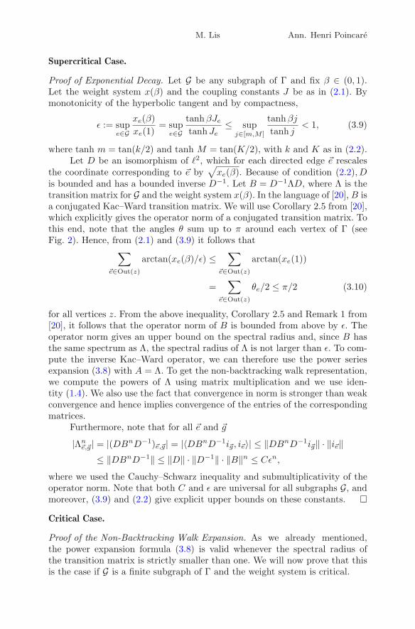
Supercritical Case.

Proof of Exponential Decay. Let G be any subgraph of Γ and fix β ∈ (0, 1).Let the weight system x(β) and the coupling constants J be as in (2.1). Bymonotonicity of the hyperbolic tangent and by compactness,

ε := supe∈G

xe(β)xe(1)

= supe∈G

tanh βJe

tanhJe≤ sup

j∈[m,M ]

tanhβj

tanh j< 1, (3.9)

where tanh m = tan(k/2) and tanh M = tan(K/2), with k and K as in (2.2).Let D be an isomorphism of �2, which for each directed edge �e rescales

the coordinate corresponding to �e by√

xe(β). Because of condition (2.2),Dis bounded and has a bounded inverse D−1. Let B = D−1ΛD, where Λ is thetransition matrix for G and the weight system x(β). In the language of [20], B isa conjugated Kac–Ward transition matrix. We will use Corollary 2.5 from [20],which explicitly gives the operator norm of a conjugated transition matrix. Tothis end, note that the angles θ sum up to π around each vertex of Γ (seeFig. 2). Hence, from (2.1) and (3.9) it follows that∑

�e∈Out(z)

arctan(xe(β)/ε) ≤∑

�e∈Out(z)

arctan(xe(1))

=∑

�e∈Out(z)

θe/2 ≤ π/2 (3.10)

for all vertices z. From the above inequality, Corollary 2.5 and Remark 1 from[20], it follows that the operator norm of B is bounded from above by ε. Theoperator norm gives an upper bound on the spectral radius and, since B hasthe same spectrum as Λ, the spectral radius of Λ is not larger than ε. To com-pute the inverse Kac–Ward operator, we can therefore use the power seriesexpansion (3.8) with A = Λ. To get the non-backtracking walk representation,we compute the powers of Λ using matrix multiplication and we use iden-tity (1.4). We also use the fact that convergence in norm is stronger than weakconvergence and hence implies convergence of the entries of the correspondingmatrices.

Furthermore, note that for all �e and �g

|Λn�e,�g| = |(DBnD−1)�e,�g| = |〈DBnD−1i�g, i�e〉| ≤ ‖DBnD−1i�g‖ · ‖i�e‖

≤ ‖DBnD−1‖ ≤ ‖D‖ · ‖D−1‖ · ‖B‖n ≤ Cεn,

where we used the Cauchy–Schwarz inequality and submultiplicativity of theoperator norm. Note that both C and ε are universal for all subgraphs G, andmoreover, (3.9) and (2.2) give explicit upper bounds on these constants. �

Critical Case.

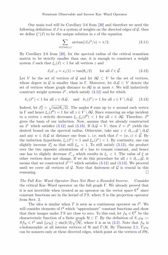
Proof of the Non-Backtracking Walk Expansion. As we already mentioned,the power expansion formula (3.8) is valid whenever the spectral radius ofthe transition matrix is strictly smaller than one. We will now prove that thisis the case if G is a finite subgraph of Γ and the weight system is critical.


Our main tool will be Corollary 2.6 from [20] and therefore we need thefollowing definition: if �x is a system of weights on the directed edges of G, thenwe define ξz(�x) to be the unique solution in s of the equation∑

�e∈Out(z)

arctan(|�x�e|2/s) = π/2. (3.11)

By Corollary 2.6 from [20], for the spectral radius of the critical transitionmatrix to be strictly smaller than one, it is enough to construct a weightsystem �x such that ξz(�x) < 1 for all vertices z and

�x�e�x−�e = xe(1) = tan(θe/2) for all �e ∈ �G. (3.12)

Let V be the set of vertices of G and let ∂G ⊂ V be the set of vertices,whose degree in G is smaller than in Γ. Moreover, let ∂rG ⊂ V denote theset of vertices whose graph distance to ∂G is at most r. We will inductivelyconstruct weight systems �xr, which satisfy (3.12) and for which

kz(�xr) < 1 for all z ∈ ∂rG, and kz(�xr) = 1 for all z ∈ V \ ∂rG. (3.13)

Indeed, let �x0�e =

√tan(θe/2). The angles θ sum up to π around each vertex

in Γ and hence ξz(�x0) = 1 for all z ∈ V \ ∂G. Since removing an edge incidentto a vertex z strictly decreases ξz, ξz(�x0) < 1 for all z ∈ ∂G. Therefore, �x0

gives the basis of our induction. Now, assume that we already constructedan �xr which satisfies (3.12) and (3.13). If ∂rG = V , then �x = �xr yields thedesired bound on the spectral radius. Otherwise, take any z ∈ ∂r+1G \ ∂rGand any w ∈ ∂rG at distance one from z, i.e. such that �e = (w, z) ∈ �G. Bythe induction hypothesis, ξz(�xr) = 1 and ξw(�xr) < 1. By continuity, one canslightly increase �xr

�e so that still ξw < 1. To still satisfy (3.12), the productover the two opposite orientations of e has to remain constant, and henceone has to slightly decrease �xr

−�e which results in ξz < 1. The value of ξ atother vertices does not change. If we do this procedure for all z ∈ ∂r+1G, itmeans that we constructed �xr+1 which satisfies (3.12) and (3.13). We proceeduntil we cover all vertices of G. Note that finiteness of G is crucial in thisreasoning. �

The Full Kac–Ward Operator Does Not Have a Bounded Inverse. Considerthe critical Kac–Ward operator on the full graph Γ. We already proved thatit is not invertible when treated as an operator on the vector space C

�Γ sinceconstant functions are in the kernel of TS, where S is the projection operatorfrom Sect. 2.

The idea is similar when T is seen as a continuous operator on �2. Wewill consider elements of �2 which “approximate” constant functions and showthat their images under TS are close to zero. To this end, let fH ∈ CΓ be thecharacteristic function of a finite graph H ⊂ Γ. By the definition of S, ϕH :=SfH ∈ �2 and ‖ϕH‖ ≥ sin(k/2)

√|H|, where k is as in (2.2). Note that fH iss-holomorphic at all interior vertices of H and Γ\H. By Theorem 2.1, TϕHcan be nonzero only at these directed edges, which point at the vertices of ∂H,


where ∂H is as in the previous proof. From the definition of the Kac–Wardoperator, it follows that

‖TϕH‖∞ ≤ Δ‖x(1)‖∞‖ϕH‖∞ ≤ tan(K/2)Δ,

where Δ is the maximal degree of Γ and K is as in (2.2). Hence,

‖TϕH‖ ≤ tan(K/2)Δ3/2√

|∂H|,which in the end yields

‖TϕH‖ ≤ C√

|∂H|/|H|‖ϕH‖,

for some constant C independent of H.It is now enough to notice that Γ admits subgraphs for which the ratio

|∂H|/|H| is arbitrarily small; it will mean that the inverse, if it exists, isunbounded in norm. To this end, one can consider subgraphs Hr, which areinduced by the vertices of Γ contained in the square [−r, r]× [−r, r]. Using con-dition (2.2), which says that all edges of Γ are surrounded by disjoint rhombiof positive minimal area (and also finite maximal area), one can prove that|∂Hr| and |Hr| grow like r and r2, respectively, when r goes to infinity. �

Acknowledgements

The author would like to thank Wouter Kager and Ronald Meester for intro-ducing him to the combinatorial aspects of the Ising model and for usefulremarks on the manuscript, and Federico Camia for the encouragement towrite this paper. The research was supported by NWO Grant Vidi 639.032.916.

References

[1] Baxter, R. J.: Free-fermion, checkerboard and Z-invariant lattice models in sta-tistical mechanics. Proc. R. Soc. Lond. Ser. A 404(1826), 1–33 (1986)

[2] Beffara, V., Duminil-Copin, H.: Smirnov’s fermionic observable away from crit-icality. Ann. Probab. 40(6), 2667–2689 (2012)

[3] Boutillier, C., de Tiliere, B.: The critical Z-invariant Ising model via dimers: theperiodic case. Probab. Theory Relat. Fields 147(3–4), 379–413 (2010)

[4] Boutillier, C., de Tiliere, B.: The critical Z-invariant Ising model via dimers:locality property. Commun. Math. Phys. 301(2), 473–516 (2011)

[5] Brydges, D., Frohlich, J., Spencer, T.: The random walk representation of classi-cal spin systems and correlation inequalities. Commun. Math. Phys. 83(1), 123–150 (1982)

[6] Chelkak, D., Hongler, C., Izyurov, K.: Conformal invariance of spin correlationsin the planar Ising model. arXiv:1202.2838 (2012)

[7] Chelkak, D., Izyurov, K.: Holomorphic spinor observables in the critical Isingmodel. Commun. Math. Phys. 322(2), 303–332 (2013)

[8] Chelkak, D., Smirnov, S.: Universality in the 2D Ising model and conformalinvariance of fermionic observables. Invent. Math. 189(3), 515–580 (2012)


[9] Cimasoni, D.: A generalized Kac–Ward formula. J. Stat. Mech. Theory E. 2010,7 (2010)

[10] Cimasoni, D., Duminil-Copin, H.: The critical temperature for the Ising modelon planar doubly periodic graphs. Electron. J. Probab. 18(44), 1–18 (2013)

[11] Dubedat, J.: Exact bosonization of the Ising model. arXiv:1112.4399 (2011)

[12] Helmuth, T.: Planar Ising model observables and non-backtracking walks.arXiv:1209.3996 (2012)

[13] Hongler, C., Kytola, K., Zahabi, A.: Discrete holomorphicity and Ising modeloperator formalism. arXiv:1211.7299 (2012)

[14] Hongler, C., Smirnov, S.: The energy density in the planar Ising model.arXiv:1008.2645 (2011)

[15] Kac, M., Ward, J.C.: A combinatorial solution of the two-dimensional Isingmodel. Phys. Rev. 88(6), 1332–1337 (1952)

[16] Kager, W., Lis, M., Meester, R.: The signed loop approach to the Ising modelFoundations and critical point. J. Stat. Phys. 152(2), 353–387 (2013)

[17] Kasteleyn, P.: The statistics of dimers on a lattice. I. The number of dimerarrangements on a quadratic lattice. Physica 27, 1209–1225 (1961)

[18] Kaufman, B.: Crystal statistics. II. Partition function evaluated by spinoranalysis. Phys. Rev. 76(8), 1232–1243 (1949)

[19] Kenyon, R.: Conformal invariance of domino tiling. Ann. Probab. 28(2), 759–795 (2000)

[20] Lis, M.: Phase transition free regions in the Ising model via the Kac–Wardoperator. arXiv:1306.2253 (2013)

[21] Onsager, L.: Crystal statistics. I. A two-dimensional model with an order-disorder transition. Phys. Rev. 65(2), 117–149 (1944)

[22] Smirnov, S.: Towards conformal invariance of 2D lattice models. In: InternationalCongress of Mathematicians, vol. II, pp. 1421–1451 (2006)

[23] Smirnov, S.: Conformal invariance in random cluster models. I. Holomorphicfermions in the Ising model. Ann. Math. (2) 172(2), 1435–1467 (2010)

[24] Whitney, H.: On regular closed curves in the plane. Compos. Math. 4, 276–284 (1937)

Marcin LisDepartment of MathematicsVU UniversityDe Boelelaan 1081a1081 HV AmsterdamThe Netherlandse-mail: [email protected]

Communicated by Denis Bernard.

Received: July 16, 2013.

Accepted: September 29, 2013.

Date post:	23-Dec-2016
Category:	Documents
Upload:	marcin
View:	214 times
Download:	2 times

The Fermionic Observable in the Ising Model and the Inverse Kac–Ward Operator

Documents