THE FETTERS OF INHERITANCE? EQUAL PARTITION AND …

Fakultät/ Zentrum/ Projekt XYInstitut/ Fachgebiet YZ

09-2019

wiso.uni-hohenheim.de

Institute of Economics

Hohenheim Discussion Papers in Business, Economics and Social Sciences

THE FETTERS OF INHERITANCE?EQUAL PARTITION AND REGIONAL ECONOMIC DEVELOPMENTThilo R. HuningUniversity of York

Fabian WahlUniversity of Hohenheim

Discussion Paper 09-2019

THE FETTERS OF INHERITANCE? EQUAL PARTITION AND REGIONAL ECONOMIC DEVELOPMENT

Thilo R. Huning, Fabian Wahl

Download this Discussion Paper from our homepage:

https://wiso.uni-hohenheim.de/papers

ISSN 2364-2084

Die Hohenheim Discussion Papers in Business, Economics and Social Sciences dienen der

schnellen Verbreitung von Forschungsarbeiten der Fakultät Wirtschafts- und Sozialwissenschaften. Die Beiträge liegen in alleiniger Verantwortung der Autoren und stellen nicht notwendigerweise die

Meinung der Fakultät Wirtschafts- und Sozialwissenschaften dar.

Hohenheim Discussion Papers in Business, Economics and Social Sciences are intended to make results of the Faculty of Business, Economics and Social Sciences research available to the public in

order to encourage scientific discussion and suggestions for revisions. The authors are solely responsible for the contents which do not necessarily represent the opinion of the Faculty of Business,

Economics and Social Sciences.

https://wiso.uni-hohenheim.de/papers

EQUAL PARTITION AND REGIONAL DEVELOPMENT

This version: July 31, 2019

The Fetters of Inheritance?Equal Partition and Regional Economic

Development*

THILO R. HUNING† FABIAN WAHL‡

Abstract

How can agricultural inheritance traditions affect structural change and economic development in ruralareas? The most prominent historical traditions are primogeniture, where the oldest son inherits the wholefarm, and equal partition, where land is split and each heir inherits an equal share. In this paper, we providea theoretical model that links these inheritance traditions to the local allocation of labor and capital and tomunicipal development. First, we show that among contemporary municipalities in West Germany, equalpartition is significantly related to measures of economic development. Second, we conduct OLS and fuzzyspatial RDD estimates for Baden-Wurttemberg in the 1950s and today. We find that inheritance rulescaused, in line with our theoretical predictions, higher incomes, population densities, and industrializationlevels in areas with equal partition. Results suggest that more than a third of the overall inter-regionaldifference in average per capita income in present-day Baden Wurttemberg, or 597 Euro, can be explainedby equal partition.

JEL Codes: D02 · D82 · H11 · H21 · N93Keywords: Inheritance rules · sectoral change · regional economic development · Baden-Wurttemberg ·

spatial inequalities

*We would like to thank Sibylle Lehmann-Hasemeyer, Nikolaus Wolf, Eric Chaney, Giacomo De Luca, AlexanderDonges, Steven Pfaff, Ulrich Pfister, Andrew Pickering, Yannay Spitzer, Jochen Streb, Max Winkler, Nathan Nunn, Se-bastian Braun and Sascha Becker. We also thank seminar participants in York, Hohenheim and Gottingen as well as theparticipants of the III. Congress on Economic and Social History 2019 in Regensburg and the 18th Annual ASREC Con-ference 2019 in Boston, especially Jared Rubin and Mark Koyama, the 2nd Workshop on Geodata in Economics 2019 inHamburg especially Stefano Falcone, Maxim Pinkovskiy and David Weil, and the 23rd SIOE Conference 2019 in Stock-holm.

†Thilo R. Huning is lecturer at Department for Economics and Related Studies, University of York, Hesligton, YorkYO10 5DD, UK; e-mail: thilo.huning at york.ac.uk

‡Fabian Wahl is post doctoral researcher at the Institute for Economic and Social History with Agricultural History,University of Hohenheim, Wollgrasweg 49, 70599 Stuttgart, Germany; e-mail: fabian.wahl at uni-hohenheim.de

1


THIS PAPER MAKES FOUR NOVEL CONTRIBUTIONS to the literature on the influence of informalinstitutions on economic development. First, we argue that particular types of social norms, agri-cultural inheritance traditions, like primogeniture and equal partition, have a profound and per-sistent effect on economic development. We show, based on historical and theoretical arguments,that equal partition is more favorable for regional industrialization and development.

Second, we derive a neoclassical model in which we allow a Malthusian economy to feature thesedifferent inheritance traditions, and in a second step to be capitalized from outside. This mod-els the historic experience of the rural areas. The putting-out system gave employment to therural population, which in turn was more willing to take this employment in areas of equal parti-tion.

As third contribution, our results imply that equal partition is an institution that reduces spatiallabor mobility but, counter-intuitively, aids economic development. This is an interesting additionto the literature around the ‘Oswald hypothesis’ (Oswald 1996).

Fourth, to our knowledge, this research is one of the first attempts to investigate systematically thelong-run development of rural areas. This is crucial for the understanding of regional economicdevelopment, as historically most of the population lived in rural areas or small towns and not inlarge cities. Yet, cities have received most of the attention of research so far (Bosker, Buringh, andVan Zanden 2013; Bosker and Buringh 2017; Borner and Severgnini 2014; Dittmar and Meisenzahl2017; Jacob 2010).

Agricultural inheritance traditions have raised ample speculations about their consequences, em-pirical studies however are rare. Ekelund, Hebert, and Tollison (2002) conduct a descriptive cross-country analysis and argue that Protestantism could spread easier into the equal partition area be-cause of their more flexible, heterogeneous and unstable societies. More recently Rink and Hilbig(2018), also using data from Baden-Wurttemberg, study the link between inheritance traditions,economic inequality and pro-egalitarian preferences.1

Historians such as Wehler (2008) view the German industrialization as a rural, and not an urban,phenomenon. He argues that the industrialization of Germany avoided cities’ regulated labormarkets by capitalizing the countryside using the putting-out system. We confirm this historicalliterature by showing theoretically that the putting-out system was likely to be more developed inareas of equal partition. Only there, because of smaller farm sizes, more farmers engaged in part-time farming and needed non-agricultural sources of income to survive. Our aim is to re-introducethis perspective into the old debate about the origins, causes, and spread of the industrializationof European countries. As such, we view the geographic pattern of economic activity in Baden-Wurttemberg today as an outcome of the interaction between local inheritance norms and theputting-out system.

We show this interaction in a standard neoclassical model of the rural economy. In the model, thebasic inheritance traditions (primogeniture or equal partition) decide the allocation of capital andlabor among families. The inheritance traditions influence the decision to allocate labor betweenthe agricultural and the industrial sector but also migration patterns. Inheritance traditions aretherefore decisive for population growth and industrialization of rural villages. Our model is the

1. Menchik (1980), in a similar attempt, studied the influence of inheritance traditions for the wealth distribution in theUnited States.

2


first to analyze the theoretical implications of equal partition on development outcomes. Existingtheoretical research has focused on the influence of primogeniture on intergenerational inequalityand social mobility (Blinder 1973; Chu 1991).

We test this theory empirically on three different datasets. First, we use the data by Rink and Hilbig(2018), who have digitized a map on inheritance traditions in West German municipalities in theearly 1950s based on a survey conducted by Rohm (1957). We find strong, robust, and positivecorrelations between equal partition and higher municipal population density and between equalpartition and wage income in 2014. This dataset has the downside that it links the tradition inhistorical municipalities with modern municipality borders. This induces the bias that territorialreforms after 1953 affected differently developed regions differently, and thus biases the data wheneconomic development is the outcome. This dataset also does not include transitional or mixedinheritance forms although they are widespread and of potential importance.

Since we are interested in regional development, we presume that credible identification of a sin-gle factor’s role for regional economic development for the whole of Western Germany is almostimpossible, given its history as one of the most fragmented regions in the world, the immigra-tion of German refugees after World War II, the variation in aerial bombing, and coal and otherresources for the rise and demise of the Ruhr area. We base the core of our analysis on the datasetby Rohm (1957), and focus on the German federal state of Baden-Wurttemberg and digitized theborders of the 3,382 historical municipalities of Baden-Wurttemberg in 1953. Focusing on Baden-Wurttemberg is interesting from a development perspective and with an eye on identification.It was not an early center of industrialization in Germany and remained an agrarian, rural stateuntil the late 19th century. Since then it has become one of the economically most prosperousand innovative regions in Germany and the whole of Europe. It is famous for its uniquely de-centralized industrial structure with small and mediums sized firms spread over urban and ruralareas. Baden-Wurttemberg today tops the German productivity statistics in the craftmanship sec-tor2. From the perspective of identification, and causal inference, the focus on Baden-Wurttembergcomes with three major advantages. First, there was just a single state government. Second, itsindustrialization coincided with the collection of reliable small-scale statistics. Third, it providesus with small-scale variation in inheritance traditions including not only the basic forms but alsoa lot of transitional and mixed traditions. Furthermore, Baden-Wurttemberg is the only area withan identifiable border between inheritance traditions in Germany, while other areas show no clearspatial distribution patterns.

We exploit this spatial discontinuity using a fuzzy spatial RDD approach. We consider economicoutcomes from the early 1950s as dependent variables. Our fuzzy RDD results imply that equalpartition municipalities have smaller farms, are significantly more industrialized, show higherpopulation densities and have more positive inter-regional migration balances. Those results arerobust to a host of robustness checks including placebo border tests, or “Donut-RDDs” (wherewe leave out the border municipalities). They also remain intact when using economic outcomesfrom 1961 as dependent variables and when controlling for coal and historical market potential.A test of the degree of selection on unobservables relative to observables necessary to explainaway the results (Altonji et al. 2015), shows that remaining unobserved heterogeneity has to be

2. Statistical Office of Baden-Wurttemberg, https://www.statistik-bw.de/Presse/Pressemitteilungen/2016330. Thislead survives adjusting for purchasing power. Data from GfK Kaufkraft Deutschland 2015

3


unlikely large (around 3 times larger as selection on observables) to undo our results. Finally,we consider contemporary municipalities and outcomes from Baden-Wurttemberg and run sharpRDDs exploiting the historical border. We find that contemporary municipalities in the historicalequal partition area have higher per capita incomes and industrial activity.

As a third dataset, we digitized data from Krafft (1930) and create a dataset for 1895 Wurttemberg.We find that our results also hold for an earlier period and with different data on local inheritancetraditions. Equal partition had led to smaller farm sizes and had a positive effect on populationdensities and municipal industrialization already before the turn of the century.

The rest of the paper has the following structure. In section I, we summarize the literature onthe consequences of inheritance traditions on economic development, followed by our model insection II. In section III, we introduce our data. To link these traditions to economic development,we provide a model in section II, and provide some empirical evidence for this idea in section IV.We conclude in section V.

I. LITERATURE REVIEW

Economic historians proposed ample theories linking inheritance practice to economic develop-ment. O’Brien (1996) hypothesizes that landless workers, which were more prevalent in primo-geniture England, provided the industrializing cities with cheap labor, and allowed it to overtakeFrance—which relied on equal partition, especially after its 1789 revolution guided by egalitarianideas of land distribution (see Tocqueville 1835).

An alternative view, dominant but not exclusively prevalent in the German-speaking literature(e.g., Habakkuk 1955; Karg 1932; Rohm 1957; Schroder 1980) is that equal partition fostered in-dustrial development. The first wave of rural industrialization was usually the establishment ofputting-out systems by one or more entrepreneurs who provided farmers with raw materials (e.g.tobacco leafs), sometimes even tools, and required them to perform certain manual tasks (e.g.rolling cigars) in a predetermined time frame.3 Wehler (2008, p. 94) argues that employees fromrural regions had two main advantages for the entrepreneurs. First, they avoided the regulationof city guilds which were hard to get into, and had highly regulated wages and labor standards.Second, peasants were seasonally unemployed for most of the year, and were seeking other modesof employment, also to hedge against the risk of harvest failure. Workers were, in Wehler’s view,exploited by low wages, long and unregulated working hours, high interests on the raw materialsto penalize lateness, and payment in kind instead of coin. All these aspects, however point at eco-nomic development in the countryside, as the potential of the rural areas is exploited, especially inareas were guilds were very restrictive at the time. When the factory overtook the putting-out sys-tem, which was prevalent until the first half of the 20th century, transport infrastructure allowedthe rural population in areas of equal partition to commute rather than to migrate.

In areas of primogeniture, putting-out systems were less successful. Siblings necessary for work-ing on the farm were more prone to these exploitative conditions, and given their more mobileinheritance, often in forms of animals or even money, could leave the municipality, and rathermove into cities. Hence, such areas would have been subject to a higher emigration, therefore we

3. See for example Karg (1932), who provides a detailed case study on the putting-out system and its connection to equalpartition for early 20th century Baden.

4


expect these areas to be less populous.4 Among others, Wegge (1998), Karg (1932) (for Baden) andKrafft (1930) (for Wurttemberg) provide historical evidence on this out-migration from the primo-geniture area.5 The migration from rural primogeniture areas to populous equal partition areasput population growth on hold or into decline in the primogeniture areas but led to a popula-tion increase in the industrializing areas of equal partition. People migrated from the agriculturalsector in the primogeniture area and engaged in industrial activities, while people who stayed inthe primogeniture area remained mostly farmers. This way, it contributed not only to structuralchange in the equal partition area but also to an increase in population density there. This createdagglomeration externalities, which fostered the industrialization of the area even further.

There is a close relation of our theory to other two sector models of urban and rural labor markets,going back to Harris and Todaro (1970). We focus however on the rural sector alone and areinterested in differences caused within this sector but across regions that apply different traditions.We introduce our idea of inheritance traditions and the role of the putting-out system.

Another idea related to this paper is that immobile property affects economic growth, knownas the Oswald-hypothesis (Oswald 1996). Proponents of this idea believe that homeownershipinduces labor market frictions, causes unemployment, and hampers economic growth.6 Our ar-gument runs in the opposite direction. In the long run, ownership of immobile capital can fostereconomic growth—given that the initial distribution of population is not inefficient. In a nutshell,our argument is that the land endowment of peasant families with in equal partition areas was of-ten too small to subsist on it but too much to entirely abandon the farm. Therefore, they suppliedcheap and skilled labor in rural areas. This allowed these regions to industrialize, and to overtakethe primogeniture areas.

The literature on agricultural inheritance traditions (e.g., Rink and Hilbig 2018; Rohm 1957) inBaden-Wurttemberg has highlighted that they were slow to adapt to the changes of the industrialrevolution and were more or less stable over time before. In Huning and Wahl (2019a) we testthis claim in a structured way, and find suggestive evidence that the general regional patterns ofinheritance traditions have been established by the early Middle Ages.

II. A MODEL ON THE ECONOMIC CONSEQUENCES OF AGRICULTURAL

INHERITANCE TRADITIONS

The implications of inheritance traditions, their advantages and disadvantages, and their role forlong-run economic development are theoretically complex. Generations of individuals applyingthem could not foresee all their consequences.

In a first step, we set up a common neoclassical model with customary notation and a small rural

4. Habakkuk (1955, pp.9) highlighting the smaller migration pressure and the less mobile inheritance of children in theequal partition area puts it like this “Where the peasant population was relatively dense but immobile, industry tended tomove to the labor; where the peasant population was more mobile even if less fertile, the industrialist had much greaterfreedom to choose his site with reference to the other relevant considerations.” He also shows that the textile industry inEngland flourished most in East Anglia, a region where equal partition was common.

5. Sering and von Dietze (1930) provide evidence that actually, the non-inheriting children often did work outside theagricultural sector, as civil servants or as craftsmen. If they however stayed in the rural area they often married (in the caseof daughters) into another farm, bought one or remained at the family farm to help their sibling and his family.

6. Wolf and Caruana-Galizia (2015) test this for Germany, and using an instrumental variable approach find that home-ownership is positively linked to unemployment.

5


wage-taking world, with given technology. We take fertility as exogenous, ignore heterogeneouspreferences and heterogeneous skills, model savings as simple as possible, and rule out economicsof scale altogether. In a second step, we trace this model through three stages of economic devel-opment. First, we sketch a Malthusian rural society in which there is no capital in the commonsense, but all material assets are employed in agriculture. In a second stage, we model the putting-system. Capitalists enter our world from the outside and settle where the provision of labor ischeapest. We show how capital is employed in areas of equal partition rather than primogeniture.In our conclusion, we argue that in the modern world with and better transport technology thispattern is likely to persist.

To abstract from individuals, our main unit of analysis is the family, which allocates resourcestogether, and can procreate. A family consists of a husband a wife, and children that are underage. Once these children get to age, they leave their core family and form a new family. This newfamily is distinct from its parents’ family, but remains related by blood to their parent family andtheir siblings’ families. The set of all families is given by the set I = {i, j, k, ...}, and these familieslive each in one village from our universe of many rural villages. We assume families have thefollowing stages of life

1. Marry & Inherit. A family is formed from two families’ children, of which one is endowedwith the production factors it inherits from its parents’ generation. In addition, the familygets one unit of labor.

2. Decide where to live and work. Families maximize their income by allocating these factorsto working in manufacturing or agriculture. If they have agricultural capital (e.g. land andtools), they have a farm. If they have other forms of capital, they can run a firm.

3. Procreate and Retire. Families get children and raise them to marriage age, to which theypass on their production factors and live with them until they die.

The historical setting of a rural economy inspires some assumptions on the productivity of familieswhen working on a farm or in a firm, which depends on the relation between the employer andthe employed, and also on the distance between the village they live and work in.

1. Families that work on their own farm, or work in their own firm, have the highest produc-tivity π = 1. This draws from the idea that parents prepare their children for their workinglives, and have a sufficient level of expertise in working on their farm or in their firm.

2. Families that work on a farm or in a firm (a) owned by someone they are related with byblood or law and (b) that lives in the same village, have a strictly lower productivity, andwe can assume from their childhood that there is also an order between brothers in terms ofproductivity. When parents retire, the second oldest child has witnessed his parents workfor longer than any of his siblings, so that we can assume that his productivity is smaller,and so forth.

3. Families from the same village but not related by blood nor law have a strictly lower produc-tivity than anyone related to the owner of the farm or firm. They might be not acquaintedwith the tasks, and might have to travel also between the work place and their home.

4. An even lower productivity have all families that have to commute to another village for

6


working on a firm or in a firm, and this commuting is so costly that being related doesn’tmake a difference anymore.

1. Farms

Farms create output by combining agricultural capital S with labor. Any family i can use itsendowment with agricultural capital S ≥ 0 (the land, the tools, the barn and stable, etc.) byemploying any family j, working on this farm Li

j ≥ 0, to create agricultural output f with givenlabor income share α,

fi =

⎛⎝∑

j∈I

πijL

ij

⎞⎠

α

S(1−α)i , (1)

while i can be the same family as j (a self-employed farmer). If the farms employ other families,family j receives a wage equal its marginal product of labor,

vij =∂Fj

∂Lij

if i �= j (2)

so that the farm’s profit is given by

Fi =

⎛⎝∑

j∈I

πijL

ij

⎞⎠

α

S(1−α)i −

∑j∈I,i �=j

vijLij . (3)

2. Manufacturing

Aside from agricultural capital, there is also classical capital K, utilized in firms. Firms createoutput by combining it with any family’s labor Li

j∗ ≥ 0, to create output m at their family-specific

technology Ai > 1 and labor income share β,

mi = Ai

⎛⎝∑

j∈I

πijL

ij

∗⎞⎠

β

K(1−β)i , (4)

wages in manufacturing w are also given by the marginal product of labor,

wij =

∂mi

∂Lij∗ , (5)

so that a firm’s profit is given by

Ri = Ai

⎛⎝∑

j∈I

πijL

ij

∗⎞⎠

β

K(1−β)i −

∑j∈I,i �=j

wijL

ij

∗. (6)

7


3. Land and Capital Markets

Families trade land and capital between themselves, under the following considerations.

1. Moving capital K from one village to another is costly. Capital is not held in stable cur-rency, but needs to be mobilized, e.g. by selling off machines, or moving them physically, attransport costs. We can assume these costs are a constant share of the units of capital sold(iceberg-type).

2. It is also costly to sell off agricultural capital S or transfer capital between S and C. Forexample, sold land might be far away from the buyer’s farm, so that for any task performedduring sowing and harvest the buyer faces long periods of traveling between lands. Addi-tionally, the buyer needs to have the financial means to acquire it. This induces a dilemma.Small pieces of land find a buyer more easily, but induce lots of traveling between fields,larger plots are too costly for anyone, and we know that pooling financial resources acrossfamilies was not common. Historical accounts highlight this physically induced barrier toland markets, and speak of this as a main reason for the immobility of the peasants.

3.1 Overall Income

Altogether, families gain income Y from wages in agriculture and manufacturing, and the profitof the farm and the firm they might own,

Yi =

⎛⎝∑

j∈I

vjiLji + wj

iLji

∗⎞⎠+ Fi +Ri (7)

4. Saving, Consuming, and Passing Down

Families consume a share of their income, and put the rest in their savings I . Consumption issome fixed amount C0 which we refer to as subsistence, and a fixed share of the excess income,0 ≤ c < 1. A family’s savings are the sum of all forms of income: wages (in agriculture and inmanufacturing), capital and land rents,

Ii = (1− c)Yi − C0 (8)

Families gain utility by leaving behind their savings to their offspring, and seek to distribute theirsavings equally across their children. They follow inheritance traditions for the distribution ofland to their children, but aim to offset the disadvantage to their children by leaving behind cap-ital. If they are themselves endowed with land, they invest a given share of their savings a intoimprovements of the farm (e.g. by purchasing more land, improve the production). All savingsthey deem not necessary for the existence of the farm, they store in capital (e.g. improvement ofthe family business, a house, but also liquid assets), so that a family’s endowment at the end of hisworking life with soil S∗ and capital C∗ is given by

S∗i = Si + aIi K∗

i = Ki + (1− a) Ii (9)

8


Let us, for now, take that the number of children is exogenous, and unrelated to the inheritancetradition, and test this assumption in the empirical part. Families pass down their endowments tothis number of children at the end of their working lives. They apply the tradition of their village v,T = {0, 1} as follows.

5. Inheritance

Consider the inheritance procedure of any family h that wishes to retire, from the perspectiveof family i, in its position as the nth of a total of m recipients of inheritance. The inheritance ofagricultural capital S is given by tradition. If its municipality v applies equal partition Tv = 0 then

Tv = 0 : Si =S∗h

mh(10)

and

Tv = 0 : Ki =K∗

h

mh(11)

If the municipality however applies primogeniture Tv = 1, then

Tv = 1 : Si =

{S∗h if n = 1

0 else(12)

and

Tv = 1 : Ki =

⎧⎪⎪⎨⎪⎪⎩

0 if n = 1 and mh > 1K∗

h

mhif n > 1 and mh > 1

K∗h if mh = 1

(13)

6. The Optimization Problem

Our families are strict income maximizers. Provided their subsistence consumption, are indifferentbetween their own consumption and their children’ consumption,

max

(Yi +

h∑n=1

Yn

)s.t.

∑j∈I

Lji + Lj

i

∗ ≤ 1 (14)

which is given the simple structure of investment opportunities equivalent to

max (Yi) s.t.∑j∈I

Lji + Lj

i

∗ ≤ 1. (15)

9


7. Stage 1: Malthusian Era

We start to understand economic development with classical Malthusian assumptions. For gener-ations, fertility prohibited any savings, so there is no classical capital K in our universe of villages,only agricultural capital S. This implies that families

max(yi) (from (15))

max

⎛⎝⎛⎝∑

j∈I

vjiLji + wj

iLji

∗⎞⎠+ Fi +Ri

⎞⎠ (from (7))

max

⎛⎝⎛⎝∑

j∈I

vjiLji + wj

iLji

∗⎞⎠+ Fi

⎞⎠, (Ci=0)

the implications of which differ by inheritance tradition.

7.1 Primogeniture in Malthusian Times

Assume that a generation has just retired, and passed down the farm and with it, the oldest brotherand his family were endowed with S (eq. (12)). Since there was no capital to be inherited, thisfamily is the only producer among his siblings. From the property of the production function (eq.(1)) with any other family working on the farm, the return to labor diminishes. Given their higherproductivity, it is rational to employ family members related to by blood or law. Assume thatthe number of brothers is plenty, and there are several families whose wage (eq. (2)) are abovesubsistence level C0, but eventually, there are families that the farm cannot nourish. Historically,family members had to leave the farm, settling in areas where land was still available, by trying tomake a life elsewhere.7 Finally, this leaves the oldest brother’s family alone with his parents (whohave saved to subsist until they die), and the amount of brothers whose marginal product is abovesubsistence, while all others leave. Cities, especially Imperial cities, provided higher wages thatrural areas since the Black Death, and were the main destination for those whose productivity ontheir family farm did not allow them to subsist.

7.2 Equal Partition in Malthusian Times

The different inheritance practice during Malthusian times becomes clear when the amount ofchildren is above two for many generations. Following the inheritance rule

7. In Huning and Wahl (2019a), we test a couple of these historical outside options. A further discussion is providedthere.

10


Si =S∗h

mhif Tv = 0 (eq. (10))

Si =Sh + aIh

mhif Tv = 0 (eq. (8))

Si =Sh

mhif Tv = 0 (Ih = 0)

Si < Sh if Tv = 0 (mh ≥ 2)

From which follows through induction that the endowment with soil approaches zero, and even-tually are too small to yield output above subsistence. Again, if there are plots of land in ouruniverse of villages that are not utilized, these families could leave the village and settle on a newplot of land, starting a new village. In analogy to the case of primogeniture, eventually land iscompletely utilized, and these family members leave our universe of villages, again potentially tothe cities of the outside world. Compared to the primogeniture areas, the higher wage in the cityminus the costs of moving there have to be marginally higher, as all who move face the costs ofabandoning their endowment with land (at least a share of it in form of transaction costs).

7.3 Conclusion on the Malthusian Era

From these we conclude that

Lemma 1. In Malthusian times, a village with primogeniture consists only of retired families, theiroldest child, and other families they are related to by blood or law, which produce output abovetheir subsistence level.

A village with equal partition consists only of retired families, and children that were each en-dowed with enough land to subsist on. Eventually, all land is utilized for agricultural production,and the distribution of across all available land villages is equal, with population density solelydetermined by the suitability of the land S.

Comparing the endowment of generation two and following generations yields

Lemma 2. Compared to villages of equal partition, villages of primogeniture has larger land hold-ings per family, and more families helping on farms owned by other families they are related toby blood or law.

8. Stage 2: Putting-out System

Assume that our universe of villages was in stage one for some generations, and then enter somefamilies with capital endowment C = 1, we call these families capitalists, and a common technol-ogy A > 1. These families choose their village they settle in freely, and locate where they maximizetheir output. Consider family i interested in founding a firm,

11


max(yi) (from (15))

max

⎛⎝⎛⎝∑

j∈I

vjiLji + wj

iLji

∗⎞⎠+ Fi +Ri

⎞⎠ (from (7))

max

⎛⎝⎛⎝∑

j∈I

vjiLji + wj

iLji

∗⎞⎠+Ri

⎞⎠ (Fi = 0)

Assume that the number of capitalists is small enough to settle far away from each other, andthat technology A is sufficiently developed enough in relation to productivity π for working forpeople they are not related with, to ensure that all capitalists work exclusively for their firm, thisbecomes

max(yi) = (Ri) (Si = 0, Lii∗= 1)

max

⎛⎜⎝Ai

⎛⎝∑

j∈I

πijL

ij

∗⎞⎠

β

K(1−β)i −

∑j∈I,i �=j

wijL

ij

∗

⎞⎟⎠ (from (4))

This yields the two conditions that capitalists focus on, namely (1) that the quantity of labor supplyis sufficient (2) at sufficient productivity π. These factors differ between primogeniture and equalpartition, according to the discussion of the Malthusian stage. Therefore, capitalists initially settledistant from each other, so they do not compete with each other over labor, but close enoughto the labor supply. We focus on labor supply to understand the difference between inheritancetraditions.

8.1 Primogeniture and the Putting-Out System

Consider the maximization problem of family i. Apart from their old job, working on k’s farm,they can now also gain income by working in j’s firm,

max(yi) (from (15))

max

⎛⎝⎛⎝∑

j∈I

vjiLji + wj

iLji

∗⎞⎠+ Fi +Ri

⎞⎠ (from (7))

max

⎛⎝⎛⎝∑

j∈I

vjiLji + wj

iLji

∗⎞⎠+ Fi

⎞⎠ (Ci = 0)

max(vki L

ki + wj

iLji

∗+ Fi

)(I = {i, j, k})

12


Assume that manufacturing technology is low enough that for the owner of the farm, i = k, it can-not be profitable to reduce the amount of labor used there. Assuming that the farm employs otherfamilies, any labor the owner takes out of his farm reduces its overall output. This rationalizes theidea that heirs in primogeniture areas stay in agriculture full-time, without side employment inmanufacturing. Any landless family i maximizes

max(vki L

ki + wj

iLji

∗)(I = {i, j, k}, Si = 0,Ki = 0)

which means they are indifferent between working in agriculture and manufacturing exactlywhen

vki Lki = wj

iLji

∗

and therefore

∂(πki L

ki

)αS(1−α)k

∂Lki

Lki =

∂

(Ai

(πjiL

ji

∗)β

K(1−β)i

)∂Lj

i

∗ Lji

∗

(πki L

ki

)αS(1−α)k = Ai

(πjiL

ji

∗)β

K(1−β)i , (from (15))

while most of the implications come from the definition of productivity.

Lemma 3. Landless families in the primogeniture area supplies labor, conditional on one, or com-bination of the factors (2) a large enough inflow of capital relative to (a) the endowment withagricultural capital and (b) the families working for the farm they work on, (2) a large enoughlevel of manufacturing technology, (3) a small enough productivity reduction for working for acapitalist they are not related to by blood or law, and (4) provided they do not have to travel toofar to work in the firm.

8.2 Equal Partition and the Putting-Out System

From the Malthusian stage, we know that in the equal partition area all families optimize like theoldest brother of the primogeniture area. We know however that they should have considerablyless land, their farm makes a lower profit even if they are the only family working on the farm (eq.(3)), and the main reason why they did not leave their village was the loss they suffer from whenselling their land. Concerning all the factors from 3, we conclude the following.

Lemma 4. Ceteris paribus, families from villages where equal partition is applied provide laborto (1) capitalists with less capital, (2) less sophisticated technology, (3) even if they incur higherreduction in productivity when working for capitalists they are not related to by blood or law, or(4) travel further to reach a workplace, or any combination of the above.

13


8.3 Conclusion on the Putting-Out System, and Dynamics

To conclude, capitalists in a putting-out system locate where labor supply is large enough, andthis is the margin more likely the case in areas of equal partition.

Lemma 5. Labor supply for capitalists is higher in villages with equal partition, compared toprimogeniture ones, and therefore settle more likely in villages of equal partition.

Consider any family i that provides labor to the capitalists. Assume that the family’s endowmentswere such that there were no savings in the generation before, Yi = C0, the new source of incomeshould therefore allow savings (eq. 8), so that Ii > 0. This allow them to improve the farm,but given that land is completely utilized, there are limits to investing in S. It is therefore safeto assume that the family does not invest all savings into the farm (a < 1), or in the case of alandless family in the primogeniture area in establishing an own farm to begin with, so that thenext generation is endowed with capital, besides the factors its parents were endowed with. Fromlemma 5, it follows that this effect is strongest in villages of equal partition.

This implies an increase in the number of capitalists, and since those who work for the capital-ists gain all the capital, we expect capital to be more and more unequally distributed across ourvillages. Families whose grandparents were working on their own land, their parents acquiringcapital from working for the entered capitalists, can employ other families themselves, providedthey can reach the same level of technology as their parents’ employer. This captures the idea thatin areas of thriving industry, we expect also the initially completely agricultural population to jointhe ranks of capitalists, which is recorded especially for the putting-out system. The decision ofa capitalist to settle in any village in any generation implies an increase in capital holdings in thesame village in the next generation.

The fact that families accumulate capital which formerly were without capital has implicationsfor the villages around it. Consider the case of a family that lives on their parents’ farm, andthe parents were marginally too distant from capitalists to be attracted. The rising wages attractthis family, given the increase in capital stock, because labor becomes scarcer relative to capital.Villages which are very distant from the initial capitalists, remains unchanged, but the distance atwhich families are indifferent increases.

Lemma 6. There is more capital accumulated in villages of equal partition compared to villages ofprimogeniture, ceteris paribus—and the distribution of capital across villages is more unequal inareas with equal land partition. Assuming common technology for all families, capital distributionwithin villages becomes more equal over the generations.

9. Conclusion on the Model

Introducing capital leads to a new option, especially for landless families. They cannot only com-mute to villages in their proximity, but lemma 6 implies also a more unequal distribution of wagesbetween villages. The increase in income experienced from moving to another village and livethere should be initially the highest for landless families, provided that the costs of physicallymoving to an area with capitalists are small. This should induce migration from primogenitureareas to areas of equal partition.

Further technical progress has rendered the putting-out system obsolete in modern Germany. We

14


can rationalize this by assuming that knowledge spillovers, or technical progress, has given somecapitalists a better technology A, which then allows them to pay higher wages, and motivate cap-italists with weaker technology to stop producing, instead working for them. Another reason inthe model could be that the productivity loss incurred by commuting decreases, which is plausi-ble in the light of advancement in transport infrastructure and technology over the 19th centuryGermany. To conclude, these are the ideas we draw from the model that we take to the data:

Theorem. In areas of equal partition, we expect (1) a higher population density, (2) smaller farms, (3) lessfamily members helping in agriculture, (4) more manufacturing, and (5) less outmigration, ceteris paribus.

III. DATA

1. Inheritance Traditions

The core of our analysis relies on municipality level data on agricultural inheritance traditions inBaden-Wurttemberg as assembled by Rohm (1957). After World War II, the federal state of Baden-Wurttemberg was founded with 3,382 municipalities, each on average only 10.56km2 in size.8 In1953, Rohm sent a one-page questionnaire to each municipality’s major. Questions included thepredominant inheritance tradition in the municipality at the time, but also its historical origin.Respondents had to decide between a ‘main form’ (Hauptform), primogeniture or equal partition,but could also choose from different transitional and mixed forms. A transitional form could bethat small farms were subject to equal partition, while primogeniture applied for large farms. Healso asked the majors whether their municipality switched from one main form to the other withinthe last hundred years, and if so, which was the ‘original form’. Only 22 municipalities (0.7 % ofall municipalities) experienced such a change in the main form between 1850 and today. Thissuggests that the traditions were relatively persistent.9 If the majors indicated that a transitionalor mixed form was prevalent they were also asked for the ‘original’ form, either primogenitureor equal partition. An outcome of the survey was that there were almost no transitional or mixedforms in 1850. This supports the claim made by many historians that most of the transitional formshave emerged only during the 20th century (Rohm 1957; Krafft 1930; Sering and von Dietze 1930).Based on the information about the origins of mixed forms and about switches in the main formbetween 1850 and 1953, he drew the border (which he called “historical main border of inheritancerules”) between the main forms, which we exploit using a spatial RDD approach. He has drawnthe border in a way that it separates the area in which only equal partition was the originallyprevalent inheritance tradition from the area in which only primogeniture was the original form(with exclaves of the respective other form as exceptions). The downside of this approach is thatit relies on the best knowledge of the majors, and to a minor extent also on their honesty.10 Wecompare his data with other data collected earlier, to be sure that this is not a crucial issue.

The questionnaire also inquired whether commons existed and if so, if they were partitioned. Thesurvey resulted in a map depicting for each municipality, one of nine predominant inheritancetraditions each with a different color or shading (Figure A.1 in the Online Appendix shows the

8. The following paragraphs draw heavily from Huning and Wahl (2019a), a companion paper of ours in which weintroduce the inheritance data in more detail.

9. In the majority of the switches, municipalities went from equal partition to primogeniture.10. Eight years after the Nazi time, this could be a bias, because the political debate emphasized primogeniture as the

‘true’ Germanic, and therefore superior, tradition.

15


original map). It distinguishes nine inheritance practices however six of them are transitionalforms of primogeniture or equal partition and there is also a mixed tradition, we aggregate thesenine to five different inheritance traditions.11 For the following empirical analysis, we howeverstudy only the impact of one of them, equal partition, compared to all the others.

We use maps on the prevalence of inheritance traditions from 1905 as printed in Krafft (1930) andSering and von Dietze (1930) to check the validity of Rohm’s map. It distinguishes only betweenthe two basic forms of equal partition and primogeniture and mixed traditions and is based ona survey of the ministry of law of Wurttemberg asking notaries about the inheritance traditionsprevalent in their jurisdiction. The map largely confirms the location of the border andStandarderrors are clustered on county level that mixed traditions were less prevalent in 1905.12

Figure 1(a) shows a map of contemporary West German municipalities and whether they appliedequal partition (blue) or primogeniture (red) in 1953. We base those map on the dataset of theRink and Hilbig (2018) study. Figure 1(b) depicts Krafft’s map from 1905, where equal partitionmunicipalities are blue, primogeniture ones are red and mixed ones are orange. Figure 1(c) showsthe digitized version of Rohm’s map, colorized by inheritance tradition. Primogeniture is the mostfrequent, prevalent in roughly 38 % of all municipalities; transitional and mixed forms apply inaround 1⁄3 of the municipalities. Figures 1(b) and (c) also show that there are several exclaves,municipalities that apply a tradition different from all its neighbors.

2. Dependent Variables and Controls

Our data on industrialization, agriculture, employment structure and basic demography rely onthe official municipal and county statistics of Baden-Wurttemberg from 1950 and 1961 (“Gemeinde-und Kreisstatistik Baden-Wurttemberg”). The municipal statistics of 1950 also report population in1939. For information on part-time farmers, we rely on the municipal statistics from 1971/72 (Sta-tistical Office of Baden-Wurttemberg 1952, 1964, 1974). These two years are the most chronologicalclosest to Rohm’s survey. Not all information is available both in 1950 and 1961 (for example, weonly have the migration balance for 1950). For the baseline analysis, we stick to the situation in1950, the year closest to Rohm’s survey. In both 1950 and 1961, the number of municipalities differsslightly from that in 1953, as some few municipalities were merged or created in between.13

We also use contemporary data. Asatryan, Havlik, and Streif (2017) provide us with the shareof industry buildings per municipality in 2010 and income per capita in 2006 (the last full yearbefore the world financial crisis) for 1,105 municipalities. We also use the areas of municipality’sindustrial zones, which we extract from openstreetmap.org.14

11. The application of one or the other tradition was not restricted by any laws, the standard German inheritance lawwas that the farm owners would be free in their will. If farmers wished to apply primogeniture they had to register theirfarms in the “Hoferolle”, a trade register for farms, expressing their will that primogeniture law of the respective state isapplied. If they changed their mind, they still could pass the farm in another way. Farms were usually passed down to thechildren during the lifetime of the parents, at parents age around 60 (Krafft 1930), so that the oldest son would be around25 years old (Karg 1932).

12. We also had a look on the maps depicted in Huppertz (1939) and Karg (1932) to get an idea about the accuracy ofRohm’s map. From the comparison, we conclude that Rohm’s map is accurate and the most detailed available.

13. For 1971/72, the number of municipalities is much lower (around 1,200) as in 1971, a fundamental reform of theadministrative regions was conducted with the results that a lot of counties and municipalities were merged together andthe number of municipalities decreased by around 2/3. We do also not have each information for all the municipalities,which can also lead to a slightly smaller number of observations than 3,382 in some regressions.

14. Our data represents the state of 10th March 2019, 12pm. We extracted the polygon shapefile by using the QGIS plug-in

16


(a)

Inhe

rita

nce

Trad

ition

sin

Con

tem

po-

rary

Wes

t-G

erm

anM

unic

ipal

ities

afte

rR

ink

and

Hilb

ig(2

018)

(b)

Inhe

rita

nce

Prac

tices

inW

urtt

embe

rgin

1905

afte

rK

rafft

(193

0)(c

)In

heri

tanc

ePr

actic

esan

dth

eH

isto

rica

lMai

nBo

rder

ofth

eEq

ualP

artit

ion

(with

Excl

aves

)in

1953

,afte

rR

ohm

(195

7)

Not

e:Bl

uem

unic

ipal

itie

spr

edom

inan

tly

appl

yeq

ualp

arti

tion

,lig

htbl

uear

em

unic

ipal

itie

sw

ith

tran

siti

onal

form

ofeq

ualp

arti

tion

,red

ispr

imog

enit

ure,

oran

gere

pres

ents

tran

siti

onal

form

sof

Prim

ogen

itur

e.T

hegr

een

area

sin

1(c)

repr

esen

tmix

edtr

adit

ions

.The

blac

klin

ein

1(c)

deno

tes

the

hist

oric

albo

rder

ofth

eeq

ualp

arti

tion

area

base

don

Roh

m(1

957)

.

Fig

ure

1:

Reg

iona

lvar

iatio

non

inhe

rita

nce

trad

ition

from

thre

edi

ffere

ntda

tase

ts

17


Our control variables originate from a large variety of data sources. To outline our main variables,the share of a municipality’s area that is used to grow wine or fruits with intensive agriculturewe take from the official municipal statistics of 1961. Data on the location of pre-medieval forestareas were digitized from a map by Ellenberg (1990). Most historical control variables (Distanceto the closest Imperial city, historical political instability and fragmentation, location in churchterritories) were taken from Huning and Wahl (2019b). Talbert (2000) provides the distance ofa municipality to the next certain Roman road network. Data on the location of Celtic graves,and 19th railway lines is taken from maps in the “Historischer Atlas von Baden-Wurttemberg”(Historical Atlas of Baden-Wurttemberg) which we have digitized (Kommission fur geschichtlicheLandeskunde in Baden-Wurttemberg 1988). The shape of the French occupation zones comes fromSchumann (2014).

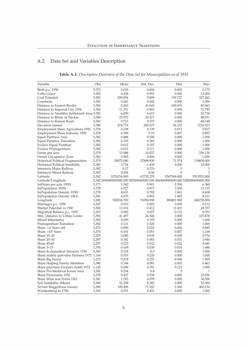
We provide a descriptive overview of all the variables in the Online Appendix in Table A.1 (for thedataset with municipalities as of 1953) and Table A.2 (for contemporary municipalities).

IV. EMPIRICAL ANALYSIS OF THE CONSEQUENCES OF AGRICULTURAL

INHERITANCE TRADITIONS

1. Results for Contemporary Municipalities and Outcomes in West Germany

We first study the effect of equal partition on economic development for the whole of West Ger-many, using data from Rink and Hilbig (2018). They digitized a map drawn by Rohm in thepublication “Atlas der deutschen Agrarlandschaft”, with data from a survey for all West Germanmunicipalities (for more details see Rink and Hilbig (2018)). They code the inheritance traditionsfor contemporary West German municipalities by overlaying Rohm’s map with a shapefile of con-temporary municipalities. Then they count the number of pixels within each current municipalityassociated with either inheritance tradition. The authors assign the inheritance tradition with thehighest share of pixels to a contemporary municipality.15 A dummy variable is obtained whichis equal to one if a contemporary municipality in 1953 applied equal partition. Figure 1(a) showsWest Germany, the borders of contemporary federal states and municipalities. In the figure, mu-nicipalities with equal partition in 1953 are blue and the ones applying primogeniture are red.A look at the map makes clear that equal partition was present mostly in Baden-Wurttemberg,Rhineland Palatine, the Saarland and the south of Hesse. It was virtually absent in Bavaria andthe north of Germany. Baden-Wurttemberg was the only state with closed equal partition and pri-mogeniture areas. All other states were scattered. We use this advantage of Baden-Wurttembergto employ a spatial RDD approach.

Their dataset also contains a host of geographical and historical control variables alongside con-temporary socio-economic outcomes (measured in 2014). Among those, the average wage incomeand population density are relevant for our analysis. These two will be the dependent variablesin OLS regressions with the equal partition dummy as variable of interest and following historicaland geographic control variables: A municipality’s distance to Wittenberg, average elevation, theintensity of the Peasant Wars of 1522-1525 in the historical state of the municipality, and dummy

QuickOSM.15. In order to arrive at a dichotomous measure, they treat transitional forms of equal partition as equal partition and

transitional forms of primogeniture as primogeniture.

18


variables for historical states of the German Empire of 1871, for municipalities historically locatedin the Roman part of Germany, and in which the code civil was the prevailing law in 1894.16 Weinclude either federal state or county fixed effects into the regressions.

Table 1 reports results of the OLS regressions. Regardless of which combination of fixed effects andcontrol variables, equal partition municipalities have a statistically and economically significantlyhigher population density (around 15 to 58 %) and higher average wage incomes (around 1.6 to 5%). In conclusion, the results confirm that there is a positive relationship between equal partitionand municipal economic prosperity in today’s West Germany.

Table 1: Equal Partition and Current Municipal Development in West Germany

Dependent Variable ln(Population Density 2014) ln(Average Wage Income 2014)

(1) (2) (3) (4) (5) (6)Equal Partition 0.567*** 0.325*** 0.154*** 0.0468*** 0.0211*** 0.0159***

(0.0754) (0.065) (0.054) (0.009) (0.006) (0.006)Federal State Dummies Yes No No Yes No NoLatitude and Longitude Yes No No Yes No NoCounty Dummies No Yes Yes No Yes YesFurther Controls No No Yes No No YesObservations 4,021 4,021 4,001 7,977 7,977 7,896R2 0.183 0.504 0.579 0.132 0.388 0.405

Notes. Standard errors are clustered on county (Landkreis) level are in parentheses. Coefficient is statistically differentfrom zero at the ***1 %, **5 % and *10 % level. The unit of observation is a municipality in 2014. All regressions include aconstant not reported. Controls include a municipality’s distance to Wittenberg, average elevation, a variable reporting theintensity to which the county in which a municipality is located was involved in the Peasant Wars of 1522-1525, dummyvariables for historical states of the German Empire of 1871, for municipality’s historically located in the Roman part ofGermany, for municipalities in which the code civil was the prevailing civil code in 1894.

2. Consequences of Equal Partition in Baden-Wurttemberg in 1950

2.1 OLS Results

We move the focus of our analysis to the state of Baden-Wurttemberg in 1950, and study the effectof equal partition on municipality level population and industry firm density (firms per hectare),industrial and agricultural employment shares, and migration balance per capita. We estimate thefollowing equation using OLS:

Outcomes,m =α+ βEqualPartitions,m + γ′Xs,m + δs + εs,m (16)

Where Outcomes,m represents one of the five measure of industrialization, structural change andinter-regional migration in municipality m in border segment s mentioned above. Xs,m is a vectorof control variables. We include geographic and historical variables to control for confoundingvariation representing the determinants of agricultural inheritance traditions studied in our com-panion paper (Huning and Wahl 2019a). We include controls of pre-historic/ancient (and there-fore pre-treatment) measures of economic development, urbanization and settlement history. This

16. For descriptive statistics of those variables, the reader is referred to the Data Appendix of the Rink and Hilbig (2018)paper.

19


accounts for persistence of deep historical factors of development. The geographic covariates in-clude mean elevation, terrain ruggedness, soil suitability and the share of agricultural area usedto grow wine and fruits in 1961, and distance to Rhine or Neckar.

Historical controls encompass distance to the closest Imperial city as of 1556, distance to next cer-tain Roman road, a dummy variable for municipalities with at least one Celtic grave, historicalpolitical fragmentation and instability, the share of a municipalities total area that is located inecclesiastical territories in 1556, pre-medieval forest areas, the share of Protestants in 1961 anda dummy for municipalities which belonged to the Duchy of Wurttemberg in 1789. We alsoadd a measure for distance to the closest urban center (either Freiburg, Heidelberg, Karlsruhe,Mannheim or Stuttgart), and to the rivers Rhine or the Neckar. This addresses concerns of prox-imity to a large agglomeration or to major rivers in the border’s vicinity. Furthermore, we includea dummy variable equal to one if a municipality was located in the French Occupation Zone afterWorld War II. This allows us to control for the argument by Schumann (2014) who shows that theoccupational zones led to discontinuous population growth until the 1970s (because the Frenchobjected to any immigration from territories Germany lost to Poland).

Some of these control variables are potentially bad controls. The potential bias from not control-ling for these factors however is likely larger than the bias that could arise from bad controls. Wealso add 25 border segment fixed effects (δs) to the estimation to further reduce unobserved het-erogeneity.17 We include all control variables in all of the estimations. εs,m is the error term. Table 2shows the results.

For all the dependent variables except the migration balance per capita, we find that equal parti-tion has an economically and statistically significant effect. For example, the number of firms perhectare is on average around 12% larger in the equal partition areas, and the share of workers inthe industrial sector is on average around 4% higher.

Despite the comprehensive set of control variables, there could be a bias of the OLS estimatesbecause of omitted variables. We therefore propose an alternative strategy to identify the causalrelationship between equal partition and our outcomes of interest. This identification strategycomes with its own challenges, but convinces in combination with the OLS results. In what fol-lows, we argue that the historical border of inheritance traditions as depicted in the map of Rohmis a valid border in a spatial RDD and henceforth enables us to eliminate potential biases arisingfrom unobserved heterogeneity.

17. We create those in the following way: We split the border into 25 equally large segments and then each municipalityis assigned to the segment it is closest to.

20


Ta

ble

2:

Equa

lPar

titio

nan

dIn

dust

rial

izat

ion,

Stru

ctur

alC

hang

e,an

dM

igra

tion

Patt

erns

1950

—O

LSEs

timat

ions

Dep

ende

ntV

aria

ble

ln(P

opul

atio

nD

ensi

ty19

50)

ln(F

irm

spe

rA

cre

1950

)Em

ploy

men

tSha

reIn

dust

ry19

50Em

ploy

men

tSha

reA

gric

ultu

re19

50M

igra

tion

Bala

nce

p.c.

1950

(1)

(2)

(3)

(4)

(5)

Equa

lPar

titi

on0.

132*

**0.

121*

*0.

042*

**-0

.029

***

0.00

1(0

.044

)(0

.048

)(0

.011

)(0

.011

)(0

.001

)

Bord

erSe

gmen

tFEs

(25)

��

��

�G

eogr

aphi

cC

ontr

ols

��

��

�H

isto

rica

lCon

trol

s�

��

��

Fren

chO

ZD

umm

y�

��

��

Dis

tanc

eto

Urb

anC

ente

r�

��

��

Inte

rsec

tsM

ajor

Rai

lway

��

��

�In

ters

ects

Min

orR

ailw

ay�

��

��

Obs

erva

tion

s3,

371

3,36

53,

370

3,37

03,

256

R2

0.48

80.

365

0.42

80.

438

0.41

8

Not

es.

Stan

dard

erro

rsar

ecl

uste

red

onco

unty

(Lan

dkre

is)

leve

lare

inpa

rent

hese

s.C

oeffi

cien

tis

stat

isti

cally

diff

eren

tfr

omze

roat

the

***1

%,*

*5%

and

*10

%le

vel.

The

unit

ofob

serv

atio

nis

am

unic

ipal

ity

in19

53.A

llre

gres

sion

sin

clud

ea

cons

tant

notr

epor

ted.

R2

isth

ece

nter

edR

2of

the

seco

ndst

age.

Geo

grap

hic

cont

rols

incl

ude

mea

nel

evat

ion,

terr

ain

rugg

edne

ssan

dso

ilsu

itab

ility

asw

ella

sth

esh

are

ofag

ricu

ltur

alar

eaus

edto

grow

win

ean

dfr

uits

in19

61,a

nddi

stan

ceto

Rhi

neor

Nec

kar.

His

tori

calc

ontr

ols

enco

mpa

ssdi

stan

ceto

the

clos

est

Impe

rial

city

asof

1556

,dis

tanc

eto

next

cert

ain

Rom

anro

ad,a

dum

my

vari

able

for

mun

icip

alit

ies

wit

hat

leas

ton

eC

elti

cgr

ave,

hist

oric

alpo

litic

alfr

agm

enta

tion

and

inst

abili

ty,

the

shar

eof

am

unic

ipal

itie

sar

eath

atis

loca

ted

inec

cles

iast

ical

terr

itor

ies

in15

56,

pre-

med

ieva

lfo

rest

area

s,th

esh

are

ofPr

otes

tant

sin

1961

and

adu

mm

yfo

rm

unic

ipal

itie

sw

hich

belo

nged

toth

eD

uchy

ofW

urtt

embe

rgin

1789

.

21


2.2 Identification Challenges

The validity of a spatial RDD rests on three assumptions. The border is drawn in an (economically)unsystematic way, there is no compound treatment, and there is no selective sorting (manipula-tion of the running variable). Of those three, the first two are the most critical in our context.18

The most crucial assumption is that the border is not endogenous to any unobserved factors andhence not drawn in a systematic way. We cannot proof the validity of this assumption, but we cantest whether relevant observables vary smoothly at the border. If this is not the case, it shows thatthe border is systematic, meaning it is located in an area where relevant characteristics change dis-continuously. As depicted in Figure 1(c), the border in the southeast, shaped like an inverted U, isalmost identical to the Black Forest. This border reflects discontinuous changes in other variables,such as elevation and other characteristics of relevance. Therefore, we exclude this border fromthe analysis. We also exclude the small, northern primogeniture area, since it has a long borderwith another state, Hesse. What remains is the eastern part of the border, stretching roughly fromthe south to the north of Baden-Wurttemberg, with a slight eastern-wards tendency. Rohm (1957)already noted that apparent geographical or historical features cannot explain this segment of theborder. From a historical point of view, one concern is that the line was not absolutely exogenous,as we know the exact mechanism that determined it. This makes our cultural border not a typicalcase for a spatial RDD, like an exogenously drawn political border would be.19

Regarding the determinants of the border, Schroder (1980) and Huppertz (1939) argue that cul-tural diffusion and imitation played a decisive role in the spread of equal partition in particular.Schroder (1980) develops the argument that equal partition occurred first in the wine-growing ar-eas, either as original development —or as suggested by others, based on Germanic traditions orRoman ideas of property—and spread from there fast in a classical process of cultural diffusionthrough imitation.20 The presence of exclaves, and a lot of transitional forms along the border thatis suggested by the results of Huning and Wahl (2019a) support this reasoning.21 Schroder (1980)further backs this argument by showing that equal partition emerged spontaneously in some ar-eas of the duchy of Wurttemberg. Together with the fact there seems to be no discontinuities innatural factors like soil quality or elevation along the border, this suggests that the historical bor-der resulted from idiosyncratic circumstances, which put historical diffusion in the municipalitiesnowadays located along the border on halt.Residuals from a regression in our companion paper(Huning and Wahl 2019a), where we explain the equal partition area support this notion too.22

Figure 3 visualizes them. Darker shades of red display higher residuals. The residuals of the pre-diction are largest around the border, implying that this area is among the locations in which wecan predict equal partition least good.

18. Selective sorting usually is an important issue when people are aware of the fact that treatment occurs at a certainvalue of the running variable, i.e. income or can manipulate their own values of the running variable accordingly leading toa higher density of observations around the threshold. In our case, the observations are municipalities and not individualsand the border is fuzzy and implicit making it unlikely that this is a big issue.

19. A prime example for a completely exogenous border are the African borders drawn in Berlin, see Michalopoulos(2012). For most European borders, endogeneity has been demonstrated by a variety of authors (Wolf, Schulze, and Heine-meyer 2011; Suesse 2018) however studies using RDD on them are as plentiful.

20. We discuss this idea and empirically test it in Huning and Wahl (2019a).21. Rohm (1957) puts it differently in saying that from today’s perspective inheritance traditions seem to result from

arbitrariness and randomness. From historical perspective, he argues, they seem to be characteristics of the cultural of thearea, which are transmitted from generation to generation.

22. The residuals originate from an OLS estimation of the probit regression in Table 1 of the companion paper.

22


For the eastern border segment, we show that relevant observables are continuous. We run spa-tial RDD estimations for a five and a ten kilometer buffer area around the border and also for themunicipalities immediately to the left and right of the border only. As running variable, we intro-duce a linear distance polynomial measuring distance to the border. We cluste standard errors oncounty level. We consider ten relevant, geographic, ancient, medieval and contemporary variablesas dependent ones. Among those are all the variables significantly predicting the equal partitionarea in Huning and Wahl (2019a) and, additionally the share of Protestants in 1950. Figure 2 re-ports the results. It shows the coefficient of the equal partition area dummy and 95 % confidenceintervals. We do not detect a significant discontinuity of these variables at the border.23 This re-assures us that at least a specification with only comparing municipalities directly at the borderleads to a valid spatial RDD.

Note: The figures show coefficients of the equal partition area dummy resulting from spatial RDD regressions for several bandwidth anddependent variables using a linear distance polynomial. In the case of the border municipalities sample, the coefficient is just the result of abivariate OLS regression. The shown confidence intervals are 95 % confidence intervals.

Figure 2: Testing for Discontinuities in Observables at the Border

23. In the case of soil quality, the equal split area dummy would become significant at 10 % level when focusing onthe border municipalities only. The marginally significant coefficient however would then be just because of two smallmunicipalities on the primogeniture side of the border that have extremely low soil quality values. If we remove those twomunicipalities, the coefficient turns insignificant.

23


No compound treatment means that the border between the equal partition and the primogenitureareas is not identical to any other existing or historical border of relevance. To show that this is thecase, Figure 4(a) depicts the eastern part of the equal partition border and the area of the three pre-decessor states of Baden-Wurttemberg (Baden, Hohenzollern, and Wurttemberg). The border isdifferent to one of those states and in fact cuts right through the middle of both Wurttemberg (darkblue) and Hohenzollern (light blue) with small but significant share of territory in the southeast ofBaden (gray). It is also not identical to the border of the French occupation zone after World WarII (the bold black line). Despite this, we include a dummy for municipalities in the French Zone toall the regressions. The border is also distinct from to the course of the two relevant rivers, Rhineand Neckar—although its course to some extent mirrors those of the Neckar flowing in the middleof the state. To rule out that this biases our results, we control for distance to Rhine and Neckar inour spatial RDD specifications.

Figures 4(b) and (c) overlay the borders of historical states in Baden-Wurttemberg in 1648 (afterthe Peace of Westphalia) and 1789 (close to the French Revolution). They also show the locationof Imperial cities (red) and ecclesiastical territories (blue). We can infer from those figures that theborder is also not identical to those of historical states, especially not to important ones that arerelevant for inheritance traditions like the historical Duchy of Wurttemberg (which was the largestate in the center of the area). We nevertheless include a dummy for municipalities in the Duchy ofWurttemberg in 1789, and as a robustness check, a complete set of historical state dummies.

Note: The figure shows residuals of a linear probability model explaining the historical equal partition area. The darker red themunicipalities are colored, the higher is the residual.

Figure 3: Predicted Equal Partition Area, Prediction Residuals and the Historical Inheritance Border

24


(a) The Eastern Historical Main Bor-der of Inheritance Practices, HistoricalStates and Major Rivers

(b) The Historical Border and States1648

(c) The Historical Border and States1789

Note: Figure (a) shows the eastern part of the historical border of the equal partition, and the borders of the historical states formingBaden-Wurttemberg (Baden, Hohenzollern and Wurttemberg) and two major rivers Rhine and Neckar. Figures (b) and (c) show the easternborder of equal partition and the historical states in 1648 (a) and 1789 (b), and secular states are depicted in gray, city states in red, andecclesiastical states in blue.

Figure 4: Maps of important control variables on historical borders and rivers

2.3 Estimation Approach

Intuitively, the idea of our identification strategy is to model municipal economic development asfunction of distance to the border. If equal partition has a positive effect, we expect a significantupward shift in the intercept of that function at the border. We estimate this shift in the interceptusing a spatial RDD approach or Boundary Discontinuity Design (BDD). A BDD is a special case ofa standard RDD but with a two-dimensional forcing variable (Keele and Titiunik 2014). Because ofthe transitional forms, we estimate a fuzzy BDD. This allows us to use the course of the border toidentify municipalities located either in the equal partition area or in the primogeniture area. Wethen use this variable to instrument actual prevalence of equal partition with location in the equalpartition area. A fuzzy BDD amounts to estimating a standard 2SLS model including a variablemeasuring the distance from each municipality to the closest border segment. We estimate thefollowing equations:

EqualPartitions,m =α1 + β1EqualPartitionAreas,m + f(Dm) + γ′1Xs,m + δs + εs,m (17a)

Outcomes,m =α2 + β2EqualPartitions,m + f(Dm) + γ′

2Xs,m + ζs + ηs,m (17b)

Where EqualPartitionAreas,m is a binary variable that indicates whether municipality m in bor-der segment s was located in the historical area of equal partition inheritance practices. This vari-able is used as instrument for the potentially endogenous dummy EqualPartitions,m which isequal to one if a municipality applied equal partition of agricultural inheritance by 1953. Heref(Dm) is a flexible linear function of the geodesic distance of each municipality’s border to theclosest point on the eastern part of the historical border. ‘Flexible’ means that we allow the dis-tance polynomial to differ in the treated and non-treated area by interacting the distance termswith the treatment variable. Outcomes,m are various socio-economic outcome variables in border

25


segment s in 1950 or 1961, depending on the availability of data. Xs,m is a vector of control vari-ables. We introduce the control variables below alongside the presentation of the results. They arehowever identical to those used for the OLS regressions of Table 2. δs and ζs represent five bordersegment fixed effects.

The standard spatial RDD, using geodesic distance to the border as running variable, has the re-striction that it does not take into account that municipalities with the same geodesic distanceto border can be far away from each other (because the north-south direction is not taken into ac-count). Introducing border segment fixed effects does already mitigate this problem. Additionally,we follow Dell (2010) and treat the border as a two-dimensional threshold to control for the exactgeographic location of a municipality (its longitude and latitude). We modify the 2SLS estimationas follows:

EqualPartitions,m =α1 + β1EqualPartitionAreas,m + f(xm, ym) + γ′1Xs,m + δs + εs,m (18a)

Outcomes,m =α2 + β2EqualPartitions,m + f(xm, ym) + γ′

2Xs,m + ζs + ηs,m (18b)

With f(xm, ym) we have a flexible function of a municipalities minimum longitudinal and latitu-dinal coordinates (xm and ym). We use a linear coordinates polynomial.24

We apply a semi-parametric operationalization of the fuzzy BDD, using three different band-widths (buffer areas) around the border for the estimation of the sample. These are ten and fivekilometers, and lastly only municipalities directly at the western and eastern side of the border.Figure 5(a) shows the estimation samples corresponding to the three different buffer areas. Fig-ure 5(b) shows which municipality is assigned to which of the five border segments. We clusterthe standard errors on county level to account for likely spatial correlation of inheritance prac-tices, and outcomes. In robustness checks, we also show that the results are robust to the use ofquadratic distance polynomials. We exclude exclave municipalities of the respective other inheri-tance practice from all estimations.

24. To be precise, the polynomial has the following form: f(x, y) = x+ y + xy.

26


(a) Buffer Areas around the Eastern Main Border (b) Border Segments around the Eastern Main Border

Note: These figures show the eastern part of the historical border of equal and unequal partition inheritance areas. In panel (a)municipalities to the left and right of the border are depicted in gray, those five kilometers away from the border are depicted in light-blueand those ten kilometer away in dark-blue. Panel (b) shows how municipalities in the buffer area are assigned to one of five bordersegments to which they are closest.

Figure 5: Buffer Areas and Border Segments around the Historical Main Border of Inheritance Practices

2.4 Consequences of Equal Partition for the Structure of the Agricultural Sector

Consider the consequences of inheritance traditions on the structure of agriculture in the 1950s.Table 3 shows the results of estimating equation 17 with border segment fixed effects and no othercontrols. We estimate the BDD for a ten kilometer buffer area around the eastern border of theequal partition area. We include four different dependent variables, including two measures offarm size (share of large farms and farms per hectare), the share of helping family members in allemployees in 1950, and common land as reported by Rohm (1957). Rohm (1957) argues that com-mon lands are more frequent in equal partition municipalities as they make it easier to maintainit. As expected, farms are on average significantly smaller in the equal partition area, there arefewer family members working on the farms and the probability that common land is present ina municipality is significantly higher. It is also worth noticing that the F-value of the equal par-tition area dummy in the first stage is very high all the time and well above the commonly usedthreshold of ten. This makes it a likely candidate for an instrument.

It is essential for our argument that the putting-out system was more widespread in the equalpartition area than in the areas of primogeniture. We cannot test that directly, but we have datafrom the early 1970s, which allow us to test whether there are more part-time farmers in the equalpartition area. If this is true it would imply that those part-time farmers also work as craftsmen orin the industrial sector when they do not engage in agricultural activities (e.g., during the winter).As this argument is essential for our story, we test this by running the BDD as before but this timewe also include control variables and use a linear coordinates polynomial as additional forcingvariable. We rely on the ten kilometer buffer to keep up the number of observations.

27


Table 3: Equal Partition and its Consequences for the Structure of Agriculture in Baden-Wurttemberg in1950

Dependent Variable Share ofFarms>40ha

Farms per Acre Share of HelpingFamily Members 1950

Commons

(1) (2) (3) (4)Buffer Area 10km around the borderEqual Partition -0.543*** 14.42*** -0.121*** 0.567***

(0.124) (3.889) (0.0348) (0.179)Linear Dist. Polynomial Yes Yes Yes YesBorder Segment FEs � � � �F-Value of Excluded IV 50.48 50.48 50.35 50.46Observations 869 869 869 870R2 0.04 0.09 0.054 0.088

Notes. Standard errors are clustered on county (Landkreis) level are in parentheses. Coefficient is statistically different fromzero at the ***1 %, **5 % and *10 % level. The unit of observation is a municipality in 1953. The F-Value of Excluded IVs refersto the F-values of the equal partition area dummy as instrument for equal partition in 1953 on the first stage. R2 is the centeredR2 of the second stage.

Table 4: Equal Partition and Part-time Farmers in Baden-Wurttemberg in 1972

Dependent Variable Part-timeFarmers (Share)

Mainly part-timefarmers (Share)

(1) (2) (3) (4)Buffer Area All Obs. 10km 10km 10km

Panel A: Linear Distance PolynomialEqual Partition 0.120*** 0.218*** 0.233*** 0.459***

(0.016) (0.079) (0.09) (0.103)F-Value of Excluded IV 921.86 40.99 29.85 40.11R2 0.097 0.157 0.282 0.09

Panel B: Linear Coordinates PolynomialEqual Partition 0.122*** 0.191*** 0.275*** 0.429***

(0.02) (0.053) (0.085) (0.065)F-Value of Excluded IV 604.05 80.67 29.06 83.27R2 0.114 0.26 0.223 0.029Border Segment FEs � � � �Geographic Controls – – � –Historical Controls – – � –French OZ Dummy – – � –Distance to Urban Center – – � –Intersects Major Railway – – � –Intersects Minor Railway – – � –Observations 1,114 316 314 322

Notes. Standard errors are clustered on county (Landkreis) level are in parentheses. Coefficient is statis-tically different from zero at the ***1 %, **5 % and *10 % level. The unit of observation is a municipalityin 1953. All regressions include a constant not reported. R2 is the centered R2 of the second stage. Ge-ographic controls include mean elevation, terrain ruggedness and soil suitability as well as the share ofagricultural area used to grow wine and fruits in 1961, and distance to Rhine or Neckar. Historical controlsencompass distance to the closest Imperial city as of 1556, distance to next certain Roman road, a dummyvariable for municipalities with at least one Celtic grave, historical political fragmentation and instability,the share of a municipalities area that is located in ecclesiastical territories in 1556, pre-medieval forestareas, the share of Protestants in 1961 and a dummy for municipalities which belonged to the Duchy ofWurttemberg in 1789.

28


We compare these results to simple OLS estimates including all municipalities for which data ex-ists, as shown in Table 4. The upper panel presents the results using distance to the border asforcing variable, and the lower panel reports the results with geographic coordinates as forcingvariable. The first column of the upper panel reports the coefficient of a standard 2SLS regressionwithout a forcing variable and using all municipalities for which we have data. Column (2) showsBDD estimates without controls and column (3) with controls. In the first three columns, the over-all share of part-time farmers in all farmers of a municipality in 1972 is the dependent variable, incolumn (4) we additionally inspect the share of the category of ‘mainly part-time farmers’.

In all the estimations, the share of part-time (or mainly part-time) farms is statistically significantlyhigher than in the equal partition area. Most conservatively, the results imply a share that is onaverage around 12 % (column 1). This provides robust empirical support for our argument linkingequal partition to the putting-out system, and part-time farming.

2.5 Consequences of Equal Partition for Industrialization and Structural Change

In the next step, we investigate the effects of equal partition on industrialization and structuralchange. First, we focus on its impact on measures of industrialization and urbanization, i.e. popu-lation density and (non-agricultural) firms per hectare. We estimate the same BDD specification asin Table 4. We also consider a smaller, five kilometers buffer area and look only at municipalitiesimmediately to the east and west of the border. Table 5 shows the results of those BDD estima-tions. Columns (1) to (4) report the results for the natural logarithm of population density andcolumns (5) to (8) those for ln firms per hectare. All results indicate that the equal partition area isboth economically and statistically significantly more industrialized than the primogeniture area.The most conservative estimations, where we consider the border municipalities and include allcontrols (columns (4)), suggest that on average the population density of an equal partition munic-ipality is around 84 % higher than that of a primogeniture municipality. Reassuringly, the resultsdo not depend on whether one uses a distance or a coordinates polynomial, underlining theirrobustness to a more precise modeling of geographic location.

In Table 6, we analyze the effect of equal partition on structural change and industry structure.We estimate the same BDD regressions as in the last table but now the dependent variables arethe share of employees in industry and agriculture. We find equal partition positively and sig-nificantly related to structural change, as the share of workers in industry is at 10 to 20 % higherin equal partition municipalities. The coefficients are almost unchanged by different bandwidthchoice, inclusion of control variables or different polynomials, again showing a robust effect ofequal partition on the structure of the economy.

29


Ta

ble

5:

Equa

lPar

titio

nan

dIn

dust

rial

izat

ion

inBa

den-

Wur

ttem

berg

in19

50

Dep

ende

ntV

aria

ble

ln(P

opul

atio

nD

ensi

ty19

50)

ln(F

irm

spe

rhe

ctar

e19

50)

(1)

(2)

(3)

(4)

(5)

(6)

(7)

(8)

Buff

erA

rea

10km

10km

5km

Bord

erM

unic

s10

km10

km5k

mBo

rder

Mun

ics

Pane

lA:L

inea

rD

ista

nce

Poly

nom

ial

Equa

lPar

titi

on0.

978*

**0.

665*

**0.

752*

**0.

909*

**1.

006*

**0.

641*

**0.

744*

**0.

994*

**(0

.302

)(0

.227

)(0

.247

)(0

.306

)(0

.284

)(0

.243

)(0

.276

)(0

.330

)F-

Val

ueof

Excl

uded

IV50

.37

48.4

134

.34

18.4

350

.48

48.4

134

.34

18.4

3R

20.

160

0.51

0.45

30.

450.

106

0.40

30.

336

0.33

1Pa

nelB

:Lin

ear

Coo

rdin

ates

Poly

nom

ial

Equa

lPar

titi

on1.

018*

**0.

618*

**0.

762*

**0.

837*

*0.

973*

**0.

641*

**0.

786*

**0.

969*

*(0

.252

)(0

.210

)(0

.218

)(0

.367

)(0

.224

)(0

.225

)(0

.231

)(0

.464

)F-

Val

ueof

Excl

uded

IV96

.48

68.5

458

.09

17.5

796

.60

68.5

458

.09

17.5

7R

2-0

.096

0.38

10.

283

0.32

1-0

.057

0.27

80.

184

0.21

1O

bser

vati

ons

868

865

586

267

869

865

586

267

5Bo

rder

Segm

entF

ixed

Effe

cts

��

��

��

��

Geo

grap

hic

Con

trol

s–

��

�–

��

�H

isto

rica

lCon

trol

s–

��

�–

��

�Fr

ench

OZ

Dum

my

–�

��

–�

��

Dis

tanc

eto

Urb

anC

ente

r–

��

�–

��

�In

ters

ects

Maj

orR

ailw

ay–

��

�–

��

�In

ters

ects

Min

orR

ailw

ay–

��

�–

��

�N

otes

.St

anda

rder

rors

are

clus

tere

don

coun

ty(L

andk

reis

)le

vela

rein

pare

nthe

ses.

Coe

ffici

ent

isst

atis

tica

llydi

ffer

ent

from

zero

atth

e**

*1%

,**5

%an

d*1

0%

leve

l.Th

eun

itof

obse

rvat

ion

isa

mun

icip

alit

yin

1953

.A

llre

gres

sion

sin

clud

ea

cons

tant

notr

epor

ted.

R2

isth

ece

nter

edR

2of

the

seco

ndst

age.

Geo

grap

hic

cont

rols

incl

ude

mea

nel

evat

ion,

terr

ain

rugg

edne

ssan

dso

ilsu

itab

ility

asw

ella

sth

esh

are

ofag

ricu

ltur

alar

eaus

edto

grow

win

ean

dfr

uits

in19

61,a

nddi

stan

ceto

Rhi

neor

Nec

kar.

His

tori

cal

cont

rols

enco

mpa

ssdi

stan

ceto

the

clos

estI

mpe

rial

city

asof

1556

,dis

tanc

eto

next

cert

ain

Rom

anro

ad,a

dum

my

vari

able

for

mun

icip

alit

ies

wit

hat

leas

tone

Cel

tic

grav

e,hi

stor

ical

polit

ical

frag

men

tati

onan

din

stab

ility

,the

shar

eof

am

unic

ipal

itie

sto

tala

rea

that

islo

cate

din

eccl

esia

stic

alte

rrit

orie

sin

1556

,pre

-med

ieva

lfor

esta

reas

,the

shar

eof

Prot

esta

nts

in19

61an

da

dum

my

for

mun

icip

alit

ies

whi

chbe

long

edto

the

Duc

hyof

Wur

ttem

berg

in17

89.

30


Ta

ble

6:

Equa

lPar

titio

nan

dEc

onom

icSt

ruct

ure

inBa

den-

Wur

ttem

berg

in19

50

Dep

ende

ntV

aria

ble

Empl

oym

entS

hare

Indu

stry

1950

Empl

oym

entS

hare

Agr

icul

ture

1950

(1)

(2)

(3)

(4)

(5)

(6)

(7)

(8)

Buff

erA

rea

10km

10km

5km

Bord

erM

unic

s10

km10

km5k

mBo

rder

Mun

ics

Pane

lA:L

inea

rD

ista

nce

Poly

nom

ial

Equa

lPar

titi

on0.

174*

**0.

158*

*0.

172*

*0.

205*

*-0

.218

***

-0.1

54**

-0.1

63*

-0.2

12**

(0.0

64)

(0.0

67)

(0.0

78)

(0.0

85)

(0.0

66)

(0.0

74)

(0.0

86)

(0.0

91)

F-V

alue

ofEx

clud

edIV

50.4

848

.41

34.3

418

.43

50.4

848

.41

34.3

418

.43

R2

0.21

80.

424

0.39

60.

397

0.07

30.

438

0.42

70.

429

Pane

lB:L

inea

rC

oord

inat

esPo

lyno

mia

lEq

ualP

arti

tion

0.14

4***

0.11

1**

0.10

2**

0.16

8**

-0.1

70**

*-0

.110

**-0

.115

**-0

.184

**(0

.046

)(0

.047

)(0

.048

)(0

.075

)(0

.053

)(0

.056

3)(0

.053

)(0

.084

)F-

Val

ueof

Excl

uded

IV96

.60

68.5

458

.09

17.5

796

.60

68.5

458

.09

17.5

7R

20.

030

0.31

50.

287

0.25

6-0

.032

0.36

70.

358

0.37

3O

bser

vati

ons

869

865

586

267

869

865

586

267

5Bo

rder

Segm

entF

ixed

Effe

cts

��

��

��

��

Geo

grap

hic

Con

trol

s–

��

�–

��

�H

isto

rica

lCon

trol

s–

��

�–

��

�Fr

ench

OZ

Dum

my

–�

��

–�

��

Dis

tanc

eto

Urb

anC

ente

r–

��

�–

��

�In

ters

ects

Maj

orR

ailw

ay–

��

�–

��

�In

ters

ects

Min

orR

ailw

ay–

��

�–

��

�N

otes

.St

anda

rder

rors

are

clus

tere

don

coun

ty(L

andk

reis

)le

vela

rein

pare

nthe

ses.

Coe

ffici

enti

sst

atis

tica

llydi

ffer

entf

rom

zero

atth

e**

*1%

,**5

%an

d*1

0%

leve

l.Th

eun

itof

obse

rvat

ion

isa

mun

icip

alit

yin

1953

.All

regr

essi

ons

incl

ude

aco

nsta

ntno

trep

orte

d.R

2is

the

cent

ered

R2

ofth

ese

cond

stag

e.G

eogr

aphi

cco

ntro

lsin

clud

em

ean

elev

atio

n,te

rrai

nru

gged

ness

and

soil

suit

abili

tyas

wel

las

the

shar

eof

agri

cult

ural

area

used

togr

oww

ine

and

frui

tsin

1961

,and

dist

ance

toR

hine

orN

ecka

r.H

isto

rica

lco

ntro

lsen

com

pass

dist

ance

toth

ecl

oses

tIm

peri

alci

tyas

of15

56,d

ista

nce

tone

xtce

rtai

nR

oman

road

,adu

mm

yva

riab

lefo

rm

unic

ipal

itie

sw

ith

atle

asto

neC

elti

cgr

ave,

hist

oric

alpo

litic

alfr

agm

enta

tion

and

inst

abili

ty,t

hesh

are

ofa

mun

icip

alit

ies

tota

lare

ath

atis

loca

ted

inec

cles

iast

ical

terr

itor

ies

in15

56,p

re-m

edie

valf

ores

tare

as,t

hesh

are

ofPr

otes

tant

sin

1961

and

adu

mm

yfo

rm

unic

ipal

itie

sw

hich

belo

nged

toth

eD

uchy

ofW

urtt

embe

rgin

1789

.

31


Another prediction of our model is that primogeniture leads to sizable out-migration of non-inheriting children from the rural primogeniture area into the more urbanized equal partition area.To assess whether this is true we estimate a BDD with the municipal migration balance per capitain 1950 as dependent variable (Table 7). We find our expectations confirmed as the per capita mi-gration balance of equal split municipalities is on average significantly more positive (by around 1to 2%) than those of municipalities applying another inheritance tradition. These 2 % are roughlycorresponding to an increase by one standard deviation of the per capita migration balance andthus, this is a non-negligible effect. As with the migration balance per capita however, we can-not say where the migrating people come from, this is only indirect, yet suggestive evidence formigration from the primogeniture to the equal partition area.

Table 7: Equal Partition and Inter-regional Migration in Baden-Wurttemberg in 1950

Dependent Variable MigrationBalance p.c. 1950

(1) (2) (3) (4)Buffer Area 10km 10km 5km Border Munics

Panel A: Linear Distance PolynomialEqual Partition 0.017** 0.01 0.02** 0.019**

(0.008) (0.006) (0.008) (0.01)F-Value of Excluded IV 54.47 53.75 35.41 18.83R2 -0.011 0.11 0.052 0.138

Panel B: Linear Coordinates PolynomialEqual Partition 0.012** 0.006 0.011** 0.016*

(0.005) (0.004) (0.005) (0.01)F-Value of Excluded IV 108.32 77.73 59.79 17.83R2 0.021 0.12 0.104 0.164Observations 842 839 569 261Border Segment FEs � � � �Geographic Controls – – � �Historical Controls – – � �French OZ Dummy – – � �Distance to Urban Center – – � �Intersects Major Railway – – � �Intersects Minor Railway – – � �

Notes. Standard errors are clustered on county (Landkreis) level are in parentheses. Coefficientis statistically different from zero at the ***1 %, **5 % and *10 % level. The unit of observationis a municipality in 1953. All regressions include a constant not reported. R2 is the centeredR2 of the second stage. Geographic controls include mean elevation, terrain ruggedness and soilsuitability as well as the share of agricultural area used to grow wine and fruits in 1961, distanceto Rhine or Neckar. Historical controls encompass distance to the closest Imperial city as of 1556,distance to next certain Roman road, a dummy variable for municipalities with at least one Celticgrave, historical political fragmentation and instability, the share of a municipalities total area thatis located in ecclesiastical territories in 1556, pre-medieval forest areas, the share of Protestants in1961 and a dummy for municipalities which belonged to the Duchy of Wurttemberg in 1789.

2.6 Robustness Checks

Our results are robust to various standard sensitivity tests and empirical exercises. A standardrobustness check for spatial RDDs is a placebo border test. In such a test, one shifts the border acertain amount to the north, east, west, or south and re-assigns treatment units accordingly to thenew, (placebo) treatment area. There should be no significant effect at this ‘false’ border—as it is

32


located entirely in either the treated or untreated area. In our case, we shift the border ten kilometerto the west and to the east and re-run the spatial RDDs using the ten kilometer buffer. This ensuresthat we only have observations in the equal partition or primogeniture area in the sample. We runplacebo tests with the outcome variables from Table 5, 6 and 7. We always include the full set ofcontrol variables and cluster standard errors on county level. A fuzzy RDD like we have conductedbefore would not yield reliable estimates, as the new equal partition area dummy would be a badproxy for being an actual equal partition municipality. This is because almost none of them areactually equal partition municipalities but primogeniture or transitional ones. Therefore, we canconduct this placebo test only be estimating a sharp RDD using the equal partition area dummyas treatment variable. This is however also an insightful robustness check.

We report the results of the sharp RDD using the actual equal partition area dummy as treatmentvariable in Panel A of Table 8. We consider only border municipalities for the sharp RDD asthis is the most demanding specification. Results show statistically and economically significantcoefficients that are nevertheless smaller than those got with the fuzzy-RDD. Given that a sharpBDD could be seen as an intention-to-treat model, it should give us the lower bound of the actualeffect of equal partition. Panel B of that table shows results of shifting the border ten kilometerwestwards—all observations are actually in the equal partition area. Panel C shows a shift of theborder ten kilometer eastwards—all observations are actual in the primogeniture area and PanelD the consequences of shifting the border five kilometers eastwards. Reassuringly, in both cases,almost all coefficients are very small and close to zero. There is one exception in columns (1) and(2) of Panel C, when the border is shifted eastwards, we find a marginally significant coefficientfor population and firm density. When we shift however the border five kilometer eastwards, weagain do not find significant coefficients for any variable. Thus, we should consider this a falsepositive. We can conclude from the placebo test that the baseline results seem not to be due tostatistical coincidence.

Table 9 presents the results of two further robustness checks. First, Panel A shows the result ofthe ‘Donut BDD’. This means we leave out the municipalities immediately to the east and westof the border when estimating the fuzzy BDD. This can be useful to account for selective sorting,measurement error (wrongly assigned municipalities) and to account for the fact that along theborder, it could occur that someone had a farm in the equal partition area but some of the fieldswere located in the nearby primogeniture area—introducing noise in our measure of inheritancetraditions. Because we lose a significant amount of observations by leaving out the border mu-nicipalities, we enlarge the buffer area for those regressions to twenty kilometer. All results butthose for the migration balance per capita remain intact and show statistically and economicallysignificant effects.

In Panel B, we address the concern that Stuttgart has been part of the panel but its size could beunrelated to the inheritance rule. This historical residential city, today one of the largest agglom-erations in Europe, could drive the results in favor of the equal partition area it is part of. Ourresults are robust to estimating the BDD just for the rural areas to the south and north of Stuttgart.We exclude the border segment containing Stuttgart and the eastern part of it agglomeration (thefourth in Figure 5).

33


Ta

ble

8:

Shar

pBD

Dan

dPl

aceb

oBo

rder

Dep

ende

ntV

aria

ble

ln(P

opul

atio

nD

ensi

ty19

50)

ln(F

irm

spe

rA

cre

1950

)Em

ploy

men

tSha

reIn

dust

ry19

50Em

ploy

men

tSha

reA

gric

ultu

re19

50M

igra

tion

Bala

nce

p.c.

1950

(1)

(2)

(3)

(4)

(5)

Buff

erA

rea

10km

Pane

lA:S

harp

BDD

(Bor

der

Mun

icip

alit

ies)

Equa

lPar

titi

on0.

23**

*0.

252*

*0.

052*

*-0

.054

**0.

005*

*(0

.072

)(0

.084

)(0

.019

)(0

.021

)(0

.002

)O

bser

vati

ons

267

267

267

267

261

R2

0.51

40.

399

0.49

50.

482

0.57

5Pa

nelB

:Shi

fted

10km

Wes

twar

dsEq

ualP

arti

tion

-0.0

8-0

.091

0.00

020.

001

-0.0

03(0

.1)

(0.1

14)

(0.0

1)(0

.016

)(0

.002

)O

bser

vati

ons

795

795

795

795

773

R2

0.56

50.

456

0.48

20.

460.

556

Pane

lC:S

hift

ed10

kmEa

stw

ards

Equa

lPar

titi

on0.

212*

*0.

322*

*0.

006

-0.0

270.

001

(0.0

9)(0

.124

)(0

.012

)(0

.019

)(0

.004

)O

bser

vati

ons

905

904

905

905

874

R2

0.43

40.

311

0.50

70.

474

0.43

7Pa

nelD

:Shi

fted

5km

East

war

dsEq

ualP

arti

tion

-0.0

79-0

.013

-0.0

010.

003

0.00

3(0

.097

)(0

.12)

(0.0

26)

(0.0

29)

(0.0

04)

R2

0.48

20.

364

0.50

20.

488

0.43

9O

bser

vati

ons

905

904

905

905

874

Bord

erSe

gmen

tFEs

��

��

�G

eogr

aphi

cC

ontr

ols

��

��

�H

isto

rica

lCon

trol

s�

��

��

Fren

chO

ZD

umm

y�

��

��

Dis

tanc

eto

Urb

anC

ente

r�

��

��

Inte

rsec

tsM

ajor

Rai

lway

��

��

�In

ters

ects

Min

orR

ailw

ay�

��

��

Not

es.

Stan

dard

erro

rsar

ecl

uste

red

onco

unty

(Lan

dkre

is)

leve

lare

inpa

rent

hese

s.C

oeffi

cien

tis

stat

isti

cally

diff

eren

tfr

omze

roat

the

***1

%,*

*5%

and

*10

%le

vel.

The

unit

ofob

serv

atio

nis

am

unic

ipal

ity

in19

53.

All

regr

essi

ons

incl

ude

aco

nsta

ntno

tre

port

ed.R

2is

the

cent

ered

R2

ofth

ese

cond

stag

e.G

eogr

aphi

cco

ntro

lsin

clud

em

ean

elev

atio

n,te

rrai

nru

gged

ness

and

soil

suit

abili

tyas

wel

las

the

shar

eof

agri

cult

ural

area

used

togr

oww

ine

and

frui

tsin

1961

,and

dist

ance

toR

hine

orN

ecka

r.H

isto

rica

lcon

trol

sen

com

pass

dist

ance

toth

ecl

oses

tIm

peri

alci

tyas

of15

56,d

ista

nce

tone

xtce

rtai

nR

oman

road

,adu

mm

yva

riab

lefo

rm

unic

ipal

itie

sw

ith

atle

asto

neC

elti

cgr

ave,

hist

oric

alpo

litic

alfr

agm

enta

tion

and

inst

abili

ty,t

hesh

are

ofa

mun

icip

alit

ies

tota

lar

eath

atis

loca

ted

inec

cles

iast

ical

terr

itor

ies

in15

56,p

re-m

edie

valf

ores

tare

as,t

hesh

are

ofPr

otes

tant

sin

1961

and

adu

mm

yfo

rm

unic

ipal

itie

sw

hich

belo

nged

toth

eD

uchy

ofW

urtt

embe

rgin

1789

.

34


We also choose the five kilometer buffer area to ensure that the included municipalities are furtheraway from Stuttgart and its suburbs. The resulting coefficients are highly statistically significantand of qualitatively the same size as the original ones. Hence, Stuttgart and its large agglomerationand industry area are not behind our results.

In the Online Appendix, we show the results of four more robustness checks. In Table A.4, Panel A,we present BDD estimates using 15 instead of five border segments and re-estimate the BDD fromthe baseline applying the ten kilometer buffer area. This leaves on average only 33 municipalitieson each side of the border and within each segment as observations. We find however quantita-tively and qualitatively similar results to the baseline estimates. If anything results regarding themigration balance per capita are stronger than in the baseline case and remain statistically signifi-cant. As the effect size remains large we attribute this to the low number of observations and thethe problem that maybe too less variation was left to estimate the coefficient precisely enough. InPanel B, we include dummy variables for each historical state a municipality was located in 1789to the full set of baseline controls and re-estimate the BDD. We gain virtually identical results. InPanel C, we control for coal access, as measured by the size of late carboniferous geological areasin km2, weighted by their distance to the municipality in km. We also control for market poten-tial in 1500 AD (based on the Bairoch dataset of historical city populations) which is calculatedaccording to the methodology of Crafts (2005).25 While market potential in 1500 AD is significantin two cases, coal access is never, and thus, the results are almost identical to those of the baselineestimations.26

Table A.5 in the Online Appendix presents the results of two last checks. In Panel A, we againuse the 5km buffer and include a quadratic distance polynomial instead of a linear one in theregression. Results are almost unchanged. Thus, the exact shape of the polynomial of the forcingvariable is not a decisive point for our results. Finally, in Panel B we include exclaves of therespective other basic inheritance tradition in the regression sample. As before, results changelittle with the exclaves included.

Our baseline results have proven to be robust to a battery of commonly applied and useful ro-bustness checks. This raises our confidence that the effects we have identified are actually repre-senting the effect of equal partition on industrialization and structural change and not somethingelse.

We complement our results for 1950 with results for 1961. For 1961, we do not have a migrationbalance in the official statistics but the other four outcomes from the baseline analysis (popula-tion and firm density, employment shares of industry and agriculture) we have available. Conse-quently, we present the result of BDD estimations using these four dependent variables measuredin 1961, using the five kilometer buffer and including all baseline controls. The results are avail-able in Table A.6 in the Appendix. They are qualitatively and quantitatively very similar to thosefor 1950. Thus, a potential bias from the distortions of World War II does not affect our baselineresults for 1950.

25. For a comprehensive description of both variables, the reader is referred to the Data Appendix.26. If we had included market potential in 1800 or 1900 results would be almost unaffected.

35


Ta

ble

9:

Don

utBD

Dan

dEs

timat

ion

with

outt

heBo

rder

Segm

entC

onta

inin

gSt

uttg

art

Dep

ende

ntV

aria

ble

ln(P

opul

atio

nD

ensi

ty19

50)

ln(F

irm

spe

rA

cre

1950

)Em

ploy

men

tSha

reIn

dust

ry19

50Em

ploy

men

tSha

reA

gric

ultu

re19

50M

igra

tion

Bala

nce

p.c.

1950

(1)

(2)

(3)

(4)

(5)

Pane

lA:B

uffe

rA

rea

20km

wit

hout

Bord

erM

unic

ipal

itie

sEq

ualP

arti

tion

0.52

5***

0.52

3***

0.12

7***

-0.1

05**

*0.

001

(0.1

57)

(0.1

86)

(0.0

42)

(0.0

40)

(0.0

04)

Obs

erva

tion

s1,

157

1,15

61,

157

1,15

71,

116

F-va

lue

ofEx

clud

edIV

114.

0811

3.97

114.

0811

4.08

123.

52R

20.

413

0.29

60.

377

0.39

10.

141

Pane

lB:B

uffe

rA

rea

5km

Wit

hout

3rd

Bord

erSe

gmen

tEq

ualP

arti

tion

0.73

5***

0.62

3**

0.18

4**

-0.1

94**

0.02

2**

(0.2

25)

(0.2

58)

(0.0

86)

(0.0

95)

(0.0

11)

Obs

erva

tion

s44

944

944

944

943

8F-

valu

eof

Excl

uded

IV27

.06

27.0

627

.06

27.0

626

.55

R2

0.48

90.

383

0.44

90.

479

0.04

3Bo

rder

Segm

entF

Es�

��

��

Geo

grap

hic

Con

trol

s�

��

��

His

tori

calC

ontr

ols

��

��

�Fr

ench

OZ

Dum

my

��

��

�D

ista

nce

toU

rban

Cen

ter

��

��

�In

ters

ects

Maj

orR

ailw

ay�

��

��

Inte

rsec

tsM

inor

Rai

lway

��

��

�N

otes

.St

anda

rder

rors

are

clus

tere

don

coun

ty(L

andk

reis

)le

vela

rein

pare

nthe

ses.

Coe

ffici

ent

isst

atis

tica

llydi

ffer

ent

from

zero

atth

e**

*1%

,**5

%an

d*1

0%

leve

l.Th

eun

itof

obse

rvat

ion

isa

mun

icip

alit

yin

1953

.A

llre

gres

sion

sin

clud

ea

cons

tant

not

repo

rted

.R

2is

the

cent

ered

R2

ofth

ese

cond

stag

e.G

eogr

aphi

cco

ntro

lsin

clud

em

ean

elev

atio

n,te

rrai

nru

gged

ness

and

soil

suit

abili

tyas

wel

las

the

shar

eof

agri

cult

ural

area

used

togr

oww

ine

and

frui

tsin

1961

,and

dist

ance

toR

hine

orN

ecka

r.H

isto

rica

lcon

trol

sen

com

pass

dist

ance

toth

ecl

oses

tIm

peri

alci

tyas

of15

56,d

ista

nce

tone

xtce

rtai

nR

oman

road

,adu

mm

yva

riab

lefo

rm

unic

ipal

itie

sw

ith

atle

asto

neC

elti

cgr

ave,

hist

oric

alpo

litic

alfr

agm

enta

tion

and

inst

abili

ty,t

hesh

are

ofa

mun

icip

alit

ies

tota

lar

eath

atis

loca

ted

inec

cles

iast

ical

terr

itor

ies

in15

56,p

re-m

edie

valf

ores

tare

as,t

hesh

are

ofPr

otes

tant

sin

1961

and

adu

mm

yfo

rm

unic

ipal

itie

sw

hich

belo

nged

toth

eD

uchy

ofW

urtt

embe

rgin

1789

.

36


A final check is to test how robust our BDD results are if we assume that unobserved heterogene-ity still exists. To put it different, we can ask us the following question: How large a remainingselection on unobservables has to be to make our results insignificant. Altonji et al. (2015) havesuggested a method enabling to assess selection on unobservables relative to observables neces-sary to explain away the results (assuming the actual effect is zero). Recently, Oster (2019) hasimproved their method and provides a Stata command (psacalc) which calculates a single value(called “delta”) reporting how large selection on unobservables has to be relative to selection onobservables to put results in doubt. We calculate this value for each of the sharp RDD specifica-tions in Panel A of Table 8.27 The values are 3.66 for Table 8, Panel A, column (1), 3.27 for column(2), 2.94 for column (3), 1.6 for column (4) and 10.47 for column (5). These values suggest that re-maining selection on unobservables has to be unrealistically larger than selection on observablesto make our results to become insignificant. This raises our confidence that they hold even if thereis still unobserved heterogeneity left.

3. Results for Contemporary Municipalities and Outcomes in Baden-Wurttemberg

To further test our model, we have to show that the effects of inheritance tradition persist, evenif agriculture today is of minor economic importance as a sector. This is also worthwhile investi-gating to rule out that idiosyncrasies of the 1950s and early 1960s, especially World War II and theEuropean Economic Miracle could drive our results. Furthermore, sectoral change from agricul-ture to industry and services is almost completed nowadays.

We cannot however repeat the analysis of the last section for contemporary municipalities andeconomic outcomes. At first, we do not have information on actual prevalence of inheritance tra-ditions today. Rink and Hilbig (2018) conducted qualitative interviews with present-day Germanfarmers and found that most of them still stick to the historical way of transferring their propertyto the next generation. This suggests that the overall pattern is likely the same. Regarding the ex-istence and increasing frequency of transitional and mixed forms during the early 20th this mightnot be the case. Second, as noted before, the number of municipalities has considerably declinedafter an administrative reform in the 1970s, so that today we only have around one third of themunicipalities of 1953. Considering those facts, we use a different approach for the contemporaryanalysis. We just took the borders of equal partition and assign each of today’s municipalities toeither the equal partition or primogeniture area when over 90 % of their area was located in oneor the other area. We then run a standard sharp BDD using the equal partition area dummy astreatment indicator and estimate the following equation when employing distance to the easternborder as forcing variable:

Outcomes,m =α+ βEqualPartitionAreas,m + f(Dm) + γ′Xs,m + δs + εs,m (19)

As previously, an alternative specification includes a linear polynomial in a municipality’s latitude

27. The psacalc command does not work with estimates from a 2SLS regression, which is why we cannot perform thistest on the fuzzy-RDD results. We have assumed, following the original approach of Altonji et al. (2015) that the maximumR2 that could be achieved if all unobserved heterogeneity is accounted for is 1. The values are robust to relax this andassume e.g., a maximum of 0.9. This would result in deltas even more in our favor as they would suggest that unobservedheterogeneity has to be even lager relatively to observed to undo our effects. The deltas obtained from assuming 0.9maximum R2 are available from the authors upon request.

37


and longitude as forcing variables, which modifies equation 19 to look like this (with f(xm, ym)

again being the coordinates polynomial):

Outcomes,m =α+ βEqualPartitionAreas,m + f(xm, ym) + γ′Xs,m + δs + εs,m (20)

Estimating a sharp BDD assumes that no changes in the basic form have occurred since the 19th

century although we know that such changes and transitions happened, but likely because ofendogenous reasons. In this sense, the sharp BDD captures the idea of an intention-to-treat modeland should provide us with a lower bound estimate of the effect as it assumes that municipalitiesare still treated with equal partition that in fact have transitional forms for some time now—whichshould have smaller or no effects.

We include the same control variables (included in Xs,m) as in the previous analysis for the 1950s.28

We choose a larger maximum and minimum bandwidth of 25 and five kilometer for our analy-sis, as the number of observations is lower today than it was in 1950. Unlike before, we do notcluster the standard errors on county level. The number of counties is so low today that clus-tering is not feasible anymore (in the case of five kilometer buffer area we would have just 18clusters/counties).

As dependent variables, we use the share of industrial buildings in all buildings in a municipalityin 2010 and the natural logarithm of income per capita in 2006. We also consider the share ofindustrial area in a municipality’s total area as of March 2019. Table 10 shows the results of thesharp BDD. It is organized in the same way as the previous tables. For all three outcomes, we finda positive and statistically and economically significant effect of being in the equal partition area.Municipalities in the historical equal partition area have on average an income per capita around4 % larger than those in the primogeniture area (columns (7)–(9)).

In euros, the smallest coefficient implies that in the equal partition area income per capita in 2006was around 598 euros higher on average—which is over one third of the overall difference inper capita income between both regions.29 Given that the equal partition area has around 7.4million inhabitants in 2006, this amounts to an extra of 4.4 billion of income in total. The shareof industry buildings (columns (1)–(3)) is around 0.04 percentage points larger which might seemsmall, but is a sizable effect as the average municipality has a share of 1.2 % of industry buildings(the maximum is 14.5%). The share of industrial area is on average 30 percentage points larger,which also is a large effect.

To conclude our results, the historical equal partition area is better developed a more industrializedthan the primogeniture area to the day, even though the agricultural sector and its inheritancetraditions make up only a small share of the economy. Hence, the different inheritance traditionshave led to different, persistent development path of their application areas.

28. We do not include however, the share of Protestants in 1950 and the share of agricultural areas used to grow wine andfruits.

29. Results of those regressions are not shown to save space. They are available upon request. The average difference inper capita income between the equal partition and primogeniture area in 2006 is 1,590 euros.

38


Ta

ble

10

:Eq

ualP

artit

ion

and

Con

tem

pora

ryM

unic

ipal

Dev

elop

men

tin

Bade

n-W

urtt

embe

rg

Dep

ende

ntV

aria

ble

Shar

eof

Indu

stry

Build

ings

2010

Shar

eof

Indu

stri

alA

rea

2019

ln(I

ncom

epe

rca

pita

2006

)

(1)

(2)

(3)

(4)

(5)

(6)

(7)

(8)

(9)

Buff

erA

rea

25km

15km

5km

25km

15km

5km

25km

15km

5km

Pane

lA:L

inea

rD

ista

nce

Poly

nom

ial

Equa

lPar

titi

on0.

0045

***

0.00

25*

0.00

43**

*0.

286*

*0.

286*

*0.

307*

*0.

0464

***

0.04

81**

0.03

77*

(0.0

01)

(0.0

01)

(0.0

01)

(0.1

17)

(0.1

17)

(0.1

18)

(0.0

17)

(0.0

19)

(0.0

23)

R2

0.28

00.

314

0.33

40.

160

0.16

50.

246

0.57

20.

614

0.61

2Pa

nelB

:Lin

ear

Coo

rdin

ates

Poly

nom

ial

Equa

lPar

titi

on0.

0044

***

0.00

32**

0.00

35**

0.28

4**

0.27

6**

0.22

8*0.

0658

***

0.05

65**

*0.

0393

*(0

.001

)(0

.001

)(0

.001

)(0

.111

)(0

.121

)(0

.127

)(0

.016

)(0

.019

)(0

.022

)R

20.

315

0.32

40.

360.

169

0.17

70.

250.

425

0.45

30.

522

5Bo

rder

Segm

entF

Es�

��

��

��

��

Geo

grap

hic

Con

trol

s�

��

��

��

��

His

tori

calC

ontr

ols

��

��

��

��

�Fr

ench

OZ

Dum

my

��

��

��

��

�D

ista

nce

toU

rban

Cen

ter

��

��

��

��

�O

bser

vati

ons

537

375

211

537

375

211

537

375

211

Not

es.S

tand

ard

erro

rsar

ecl

uste

red

onco

unty

(Lan

dkre

is)l

evel

are

inpa

rent

hese

s.C

oeffi

cien

tis

stat

isti

cally

diff

eren

tfro

mze

roat

the

***1

%,*

*5%

and

*10

%le

vel.

The

unit

ofob

serv

atio

nis

am

unic

ipal

ity

in19

53.

All

regr

essi

ons

incl

ude

aco

nsta

ntno

trep

orte

d.G

eogr

aphi

cco

ntro

lsin

clud

em

ean

elev

atio

n,te

rrai

nru

gged

ness

and

soil

suit

abili

tyas

wel

las

the

shar

eof

agri

cult

ural

area

used

togr

oww

ine

and

frui

tsin

1961

,and

dist

ance

toR

hine

orN

ecka

r.H

isto

rica

lcon

trol

sen

com

pass

dist

ance

toth

ecl

oses

tIm

peri

alci

tyas

of15

56,d

ista

nce

tone

xtce

rtai

nR

oman

road

,adu

mm

yva

riab

lefo

rm

unic

ipal

itie

sw

ith

atle

asto

neC

elti

cgr

ave,

hist

oric

alpo

litic

alfr

agm

enta

tion

and

inst

abili

ty,t

hesh

are

ofa

mun

icip

alit

ies

tota

lare

ath

atis

loca

ted

inec

cles

iast

ical

terr

itor

ies

in15

56,p

re-m

edie

valf

ores

tare

as,a

nda

dum

my

for

mun

icip

alit

ies

whi

chbe

long

edto

the

Duc

hyof

Wur

ttem

berg

in17

89.

39


4. Additional Results

4.1 Results for Demographic Outcomes

Based on a case study of the primogeniture area of northeastern part Wurttemberg, Krafft (1930)concluded that the number of children in the primogeniture area was smaller. He supposes thatpeople found one son enough to guarantee the future of the family property, and avoided to com-pensate the other children. Another argument brought forward by him is that the higher marriageage in the primogeniture areas limited the number of children a couple could get and contributedto the lower population growth in the primogeniture area. Other scholars argued that it could bethe other way round and equal partition lead to fewer children as parents want to restrict furtherfragmentation of property (Habakkuk 1955). Geographically more broad analyses like Sering andvon Dietze (1930) however could not find a clear relationship between inheritance traditions andfertility numbers or marriage ages. Hence, there is no consensus on whether and how inheritancetraditions influence demographic outcomes like birth rates. In Table A.7 in the Appendix, wereport the results of BDD regressions for demographic outcomes (death and birth rates, age struc-ture etc.). We do not see a large influence of equal partition on the age structure or birth and deathrates. Giving the ambiguous arguments about the influence of equal partition on these outcomesthis is not surprising.

4.2 Results for late 19th Century Wurttemberg

We now show that we find similar impacts of inheritance traditions on economic developmentwhen using alternative, and historically earlier inheritance data from Krafft (1930)30, which is for1895 but restricted to the area of Wurttemberg. Industrialization in this area was ongoing at leastsince 1850, but also as we know that the 20th century has seen the frequent emergence of transi-tional and mixed inheritance practices. Looking at an earlier period when more municipalities stillapplied the traditional basic inheritance practices primogeniture and equal partition should give aclearer picture about their effects than the more complex picture in the mid-20th century. Further-more, studying an earlier period based on a different source for the inheritance traditions, couldreassure us that our results are not depending on the particular survey of Rohm (1957).

As dependent variables, we consider population density in 1834 and 1895, and the number ofindustry firms and farms per hectare, all in 1895. Information necessary to calculate these variablescomes from the official statistics of the kingdom of Wurttemberg from 1895 (Statistical Office ofWurttemberg 1900). We use the same control variables as before, but we only consider the railwaynetwork as of 1894 and the share of Protestants in 1895 (also from the official statistics). We donot include the share of agricultural area in which wine or fruits are grown, as there is no data.Distance to urban center we adjust to take into account that the kingdom of Wurttemberg onlyhad two large urban centers, Stuttgart and Ulm.31

The Data Appendix (Table A.3) provides a descriptive overview of the dataset for 1895 Wurttemberg.

30. We thank Sebastian Braun for making available to us his shapefile of municipalities in Wurttemberg as of 1890, whichis the basis for our dataset. There were no changes in municipalities between 1890 and 1905.

31. We also include latitudinal and longitudinal coordinates of a municipality’s centroid as controls to account for generalspatial development patterns. This is important, as we are not able to include county fixed effects into the regression.Around 1900, Wurttemberg had more than 60 counties (“Oberamter”) and, based on the Krafft (1930) map, there is not alot of variation in inheritance traditions within these comparatively small counties.

40


As the map of Krafft (1930) does not include a border and given that it is unclear what the originalinheritance practice of his “mixed traditions” is, we are not able to draw one. OLS regressionsare therefore the only feasible choice. Table 11 reports the results of estimations with the equalpartition dummy as variable of interest and the four dependent variables, introduced above. Theestimated coefficients suggest that, as in 1950 and today, municipalities applying equal partitionhave significantly lower farm sizes, higher population densities and are more industrialized. Thisimplies that our results from other periods are not coincidence or depend on Rohm’s map.

Table 11: Equal Partition and Municipal Economic Development in the 19th Century Wurttemberg

Dependent Variable ln(Farms perhectare 1895)

ln(PopulationDensity 1834)

ln(PopulationDensity 1895)

ln(Firms perhectare 1895)

(1) (2) (3) (4)Equal Partition 0.357*** 0.28*** 0.282*** 0.205**

(0.067) (0.078) (0.078) (0.084)Geographic Controls � � � �Historical Controls � � � �Distance to Urban Center � � � �Intersects Major Railway � – � �Intersects Minor Railway � – � �Observations 1,828 1,828 1,828 1,316R2 0.416 0.203 0.232 0.177

Notes. Standard errors are clustered on county (Oberamt) level are in parentheses. Coefficient is statistically different from zero at the ***1%, **5 % and *10 % level. The unit of observation is a municipality in 1890. All regressions include a constant not reported. Geographiccontrols include mean elevation, terrain ruggedness and soil suitability, as well as distance to Rhine or Neckar and latitude and longitudeof a municipality’s centroid. Historical controls encompass distance to the closest Imperial city as of 1556, distance to next certain Romanroad, a dummy variable for municipalities with at least one Celtic grave, historical political fragmentation and instability, the share of amunicipalities total area that is located in ecclesiastical territories in 1556, pre-medieval forest areas, the share of Protestants in 1895 and adummy for municipalities which belonged to the Duchy of Wurttemberg in 1789.

V. CONCLUSION

In this paper, we study the consequences of agricultural traditions on the degree of industrializa-tion and structural change in the 20th and 21st century. We find, in line with our theoretical propo-sitions, equal partition is beneficial from an economic point of view, as it led to smaller farms andonly children with an inheritance. This implies that part-time farmers, that allocated a portionof their working time to non-agricultural activities, first within the rural-putting out system, andlater in factories, were the nucleus of today’s decentralized industry in Southern Germany. Equalpartition areas saw a lower level of out-migration from rural areas to industrial centers, whichallowed a higher population growth in the Post-Malthusian Era, which fostered industrialization,as shown with data from the 1950s and today.

Small-scale differences in agricultural inheritance traditions can explain the well-known, and unique,decentralized industrial structure of the area. They might also explain why its economic prosperityand high level of innovation rests on small and medium-sized firms instead of large, multinationalcompanies. Our results support the view outlined by German historians that, unlike for examplein England, the (comparatively late) industrialization of Germany was a rural phenomenon. It didnot start in places that are large cities today, but in remote areas and with small firms and part-time farmers become craftsmen, textile, or tobacco workers. This finding can shed light on the

41


development of domestic demand and industrialization processes in other world regions.

On a more general level, the paper is among the first to study the long-run development of ruralareas. Historically, most people lived in rural areas outside the large cities. Shedding light on thedevelopments in these, more remote areas is instrumental for a full understanding of the causesand diffusion of industrialization throughout Europe in the 19th and early 20th century. We hopethat this study will inspire others to have a closer look at the historical developments in ruralareas.

This paper proposes a channel through which agricultural inheritance norms affected the patternof economic development. It is a natural follow-up question to derive counterfactuals on howBaden-Wurttemberg would have developed if there was historically only one inheritance norm. Ifequal partition had for example never existed, this would have increased migration to cities. Howmuch larger would Stuttgart be today? Would Baden-Wurttemberg, or Germany, be richer now?All these questions call for more theory, and yet more data.

REFERENCES

Altonji, Joseph G., Timothy Conley, E. Elder Todd, and Christopher R. Taber. 2015. “Methodsfor Using Selection on Observed Variables to Address Selection on Unobserved Variables.”Mimeo, nos. 98-19.

Asatryan, Z., A. Havlik, and F. Streif. 2017. “Veoting and Inaugurating Policy Like Others Do:Evidence on Spatial Interactions in Voter Initiatives.” Public Choice 172:525–544.

Blinder, Alan S. 1973. “A Model of Inherited Wealth.” Quartely Journal of Economics 87 (4): 608–626.

Borner, Lars, and Battista Severgnini. 2014. “Epidemic trade.” LSE Economic History Working Papers,No. 212/2014.

Bosker, Maarten, and Eltjo Buringh. 2017. “City Seeds: Geography and the Origins of the EuropeanCity System.” Journal of Urban Economics 98:139–157.

Bosker, Maarten, Eltjo Buringh, and Jan Luiten Van Zanden. 2013. “From Baghdad to London.Unraveling Urban Development in Europe, the Middle East, and North Africa, 800–1800.”Review of Economics and Statistics 95 (4): 1418–1437.

Chu, C.Y. Cyrus. 1991. “Primogeniture.” Journal of Political Economy 99 (1): 78–99.

Crafts, Nicholas. 2005. “Market potential in British regions, 1871–1931.” Regional Studies 39 (9):1159–1166.

Dell, Melissa. 2010. “The persistent effects of Peru’s mining mita.” Econometrica 78 (6): 1863–1903.

Dittmar, Jeremiah, and Ralf R. Meisenzahl. 2017. “State Capacity and Public Goods: InstitutionalChange, Human Capital, and Growth in Historic Germany.” Mimeo.

42


Dustmann, Christian, Bernd Fitzenberger, Uta Schonberg, and Alexandra Spitz-Oener. 2014. “Fromsick man of Europe to economic superstar: Germany’s resurgent economy.” Journal of EconomicPerspectives 28 (1): 167–88.

Ekelund, Robert B, Jr, Robert F Hebert, and Robert D Tollison. 2002. “An economic analysis of theprotestant reformation.” Journal of Political Economy 110 (3): 646–671.

Ellenberg, Heinz. 1990. Bauernhaus und Landschaft in okologischer und historischer Sicht. Eugen UlmerVerlag, Stuttgart.

Habakkuk, Hrothgar J. 1955. “Family Structure and Economic Change in Nineteenth-Century Eu-rope.” Journal of Economic History 15 (1–12): 397–433.

Harris, John R., and Michael P. Todaro. 1970. “Migration, Unemployment and Development: ATwo-Sector Analysis.” The American Economic Review 60 (1): 126–142.

Huning, Thilo R., and Fabian Wahl. 2019a. “From Romans to Ruins: How flexible were WesternInheritance Traditions?” Mimeo.

. 2019b. “You Reap What You Know: Origins and Dynamics of State Capacity.” Mimeo.

Huppertz, Barthel. 1939. Raume und Schichten bauerlicher Kulturformen in Deutschland. Ein Beitragzur Deutschen Bauerngeschichte. Ludwig Rohrschild Verlag, Bonn.

Jacob, Marcus. 2010. “Long-Term Persistence: The Free and Imperial City Experience in Germany.”Mimeo.

Karg, Helmut. 1932. Der Einfluss der Industrie auf die Art der bauerlichen Vererbung, die landwirtschaftlicheBetriebsgrosse und die Landflucht in Baden. Friedrich Find Sohne, Stuttgart.

Keele, L., and R. Titiunik. 2014. “Geographic boundaries as regression discontinuites.” PoliticalAnalysis 22:814–863.

Kommission fur geschichtliche Landeskunde in Baden-Wurttemberg, ed. 1988. Historischer Atlasvon Baden-Wurttemberg. Offizin Chr. Scheufele, Stuttgart.

Krafft, Karl. 1930. Anerbensitte und Anerbenrecht in Wurttemberg: unter besonderer Berucksichtigungvon Wurttembergisch-Franken. Kohlhammer.

Melitz, Marc J. 2003. “The impact of trade on intra-industry reallocations and aggregate industryproductivity.” Econometrica 71 (6): 1695–1725.

Menchik, Paul L. 1980. “Primogeniture, Equal Sharing, and the U.S. Distribution of Wealth.” Quar-terly Journal of Economics 94 (2): 299–316.

Michalopoulos, Stelios. 2012. “The Origins of Ethnolinguistic Diversity.” American Economic Review102, no. 4 (June): 1508–39.

43


O’Brien, Patrick Karl. 1996. “Path dependency, or why Britain became an industrialized and ur-banized economy long before France.” The Economic History Review 49 (2): 213–249.

Oster, Emily. 2019. “Unobservable Selection and Coefficient Stability: Theory and Evidence.” Jour-nal of Business & Economic Statistics 37 (2): 187–204.

Oswald, Andrew J. 1996. A conjecture on the explanation for high unemployment in the industrializednations: Part I. Technical report.

Rink, Anselm, and Hanno Hilbig. 2018. “Do Inheritance Customs Affect Political and Social In-equality?” American Journal of Political Science, forthcoming.

Rohm, Helmut. 1957. Die Vererbung des landwirtschaftlichen Grundeigentums in Baden-Wurttemberg.Bundesanstalt fur Landeskunde, Remagen/Rh.

Roses, Joan, and Nikolaus Wolf. 2018. “Regional economic development in Europe, 1900-2010: adescription of the patterns.”

Schroder, Karl Heinz. 1980. “Vererbungsformen und Hofgroßen in der Landwirtschaft um 1955.”Historischer Atlas von Baden-Wurttemberg–Erlauterungen: 1–13.

Schumann, Abel. 2014. “Persistence of Population Shocks: Evidence from the Occupation of WestGermany after World War II.” American Economic Journal. Applied Economics 6:189–205.

Sering, Max, and Constantin von Dietze, eds. 1930. Die Vererbung des landlichen Grundbesitzes.Vol. Teil 1: Deutsches Reich. Duncker & Humblot, Munich / Leipzig.

Statistical Office of Baden-Wurttemberg, ed. 1952. Gemeinde- und Kreisstatistik Baden-Wurttemberg1950. Vol. 3. Statistisches Landesamt Baden-Wurttemberg, Stuttgart.

, ed. 1964. Gemeindestatistik Baden-Wurttemberg 1960/61. Vol. 1,3 and 5. Statistisches Lan-desamt Baden-Wurttemberg, Stuttgart.

, ed. 1974. Gemeindestatistik 1970. Ergebnisse der Großzahlungen 1968 bis 1971. Vol. 4b. Land-wirtschaftliche Betriebsverhaltnisse 1971/72. Statistisches Landesamt Baden-Wurttemberg,Stuttgart.

Statistical Office of Wurttemberg, ed. 1900. Die Ergebnisse der Berufs- und Gewerbezahlung von 1895 inWurttemberg. Wurttembergische Jahrbucher fur Statistik und Landeskunde. Erganzungsand.Kohlhammer, Stuttgart.

Suesse, Marvin. 2018. “Breaking the Unbreakable Union: Nationalism, Disintegration and the So-viet Economic Collapse.” Economic Journal 128, no. 615 (November): 2933–2967.

Talbert, Richard J.A, ed. 2000. Barrington Atlas of the Greek and Roman World. Princeton, NJ: Prince-ton University Press.

Tocqueville, Alexis de. 1835. De la democratie en Amerique.

44


Wegge, Simone A. 1998. “Chain Migration and Information Networks: Evidence from Nineteenth-Century Hesse-Cassel.” Journal of Economic History 58 (4): 957–986.

Wehler, Hans-Ulrich. 2008. Deutsche Gesellschaftsgeschichte. 1. Vom Feudalismus des alten Reiches biszur defensiven Modernisierung der Reformara: 1700-1815. C.H. Beck, Munich.

Wolf, Nikolaus, and Paul Caruana-Galizia. 2015. “Bombs, homes, and jobs: Revisiting the Oswaldhypothesis for Germany.” Economics Letters 135:65–68.

Wolf, Nikolaus, Max-Stephan Schulze, and Hans-Christian Heinemeyer. 2011. “On the EconomicConsequences of the Peace: Trade and Borders After Versailles.” The Journal of Economic History71, no. 04 (December): 915–949.

45

Evolution of Inheritance Traditions

Appendix (For online publication only)

A.1. The Map of Inheritance practices of Rohm (1957)

Figure A.1: Map of Inheritance Practices and Partitioned Common Land in 1953 according to Rohm(1957).

i


A.2. Data Set and Variables Description

Table A.1: Descriptive Overview of the Data Set for Municipalities as of 1953

Variable Obs Mean Std. Dev. Min Max

Birth p.c. 1950 3,372 0.019 0.006 0.002 0.175Celtic Grave 3,382 0.428 0.991 0.000 13.000Coal Potential 3,382 209.954 5.895 199.727 227.442Commons 3,382 0.267 0.442 0.000 1.000Distance to Eastern Border 3,382 -2.263 41.643 -100.476 85.063Distance to Imperial City 1556 3,382 11.331 9.843 0.000 51.745Distance to Neolithic Settlement Area 3,382 6.099 6.613 0.000 33.730Distance to Rhine or Neckar 3,380 23.572 20.471 0.000 88.011Distance to Roman Road 3,382 9.713 9.573 0.000 48.148Elevation (mean) 3,380 474.774 200.677 96.333 1216.923Employment Share Agriculture 1950 3,378 0.338 0.139 0.011 0.817Employment Share Industry 1950 3,378 0.389 0.19 0.007 0.893Equal Partition Area 3,382 0.488 0.500 0.000 1.000Equal Partition Transition 3,382 0.153 0.360 0.000 1.000Exclave Equal Partition 3,382 0.012 0.107 0.000 1.000Exclave Primogeniture 3,382 0.012 0.111 0.000 1.000Farms per acre 3,379 13.988 10.027 0.000 259.130French Occupation Zone 3,382 0.565 0.496 0.000 1.000Historical Political Fragmentation 3,379 20075.080 27898.930 71.574 118850.000Historical Political Instability 3,382 3.724 1.438 0.000 10.000Intersects Major Railway 3,382 0.17 0.376 0 1Intersects Minor Railway 3,382 0.304 0.46 0 1Latitude 3,382 5376216.000 62732.270 5267568.000 5513552.000Latitude*Longitude 3,382 2690000000000.000 287000000000.000 2060000000000.000 3280000000000.000ln(Firms per acre 1950) 3,373 1.542 0.901 -2.596 6.360ln(Population 1939) 3,378 6.527 0.973 3.258 13.115ln(Population Density 1950) 3,378 4.631 0.782 1.861 8.608ln(Population Density 1961) 3,381 4.675 0.892 1.485 8.611Longitude 3,382 500216.700 51094.990 389401.900 606720.000Marriages p.c. 1950 3,347 0.010 0.003 0.000 0.112Market Potential in 1500 3,382 13.016 0.412 12.431 18.337Migration Balance p.c. 1950 3,263 0.002 0.027 -0.132 0.353Min. Distance to Urban Center 3,382 41.497 26.546 0.000 125.878Mixed Inheritance 3,382 0.039 0.193 0.000 1.000Primogeniture Transition 3,382 0.121 0.326 0.000 1.000Share <6 Years old 3,375 0.090 0.024 0.006 0.845Share >65 Years 3,376 0.101 0.051 0.007 1.168Share 15–20 3,376 0.085 0.034 0.009 0.734Share 20–45 2,297 0.341 0.083 0.031 3.946Share 45-65 2,297 0.223 0.032 0.022 0.649Share 5–15 3,376 0.169 0.038 0.014 1.486Share Ecclesiastical Territory 1556 3,382 0.124 0.3 0.000 1.000Share mainly part-time Farmers 1972 1,164 0.553 0.220 0.000 1.000Share Big Farms 3,375 0.378 0.257 -0.006 1.909Share Helping Family Members 3,380 0.144 0.081 0.003 0.463Share part-time Farmers (total) 1972 1,145 0.686 0.181 0.121 1.000Share Pre-Medieval Forest Area 3,382 0.234 0.4 0 1Share Protestants 1950 3,378 0.437 0.538 0.000 23.056Share Wine and Fruits 1961 3,381 1.765 4.078 0.000 36.500Soil Suitability (Mean) 3,380 22.258 8.282 0.000 52.000Terrain Ruggedness (mean) 3,380 100.496 71.543 2.366 460.234Wurttemberg in 1789 3,382 0.231 0.421 0.000 1.000

ii


Table A.2: Descriptive Overview of the Data Set for Contemporary Municipalities


Celtic Grave 1,105 0.405 0.491 0.000 1.000Coal Potential 3,382 209.954 5.895 199.727 227.442Distance to Eastern Border 1,105 -2.649 40.358 -96.783 83.086Distance to Imperial City 1556 1,105 9.467 8.994 0.000 47.45Distance to Neolithic Settlement Area 1,105 4.843 6.282 0.000 31.236Distance to Rhine or Neckar 1,105 12.916 12.992 0.000 64.653Distance to Roman Road 1,105 7.865 8.446 0.000 40.900Elevation (mean) 1,101 469.448 204.369 95.824 1150.703Equal Partition Area 1,105 0.514 0.500 0.000 1.000Exclave Equal Partition 1,105 0.018 0.133 0.000 1.000Exclave Primogeniture 1,105 0.018 0.133 0.000 1.000French Occupation Zone 1,105 0.5312217 0.4992502 0 1Historical Political Fragmentation 1,105 18735.050 24752.880 108.754 99351.710Historical Political Instability 1,105 4.474 1.937 1.000 13.000ln(Income per capita 2006) 1,101 2.64 0.145 2.005 3.564Market Potential in 1500 3,382 11.72 0.307 11.412 14.332Min. Distance to Urban Center 1,105 35.920 27.763 0.000 122.201Share Ecclesiastical Territory 1556 1,105 0.128 0.28 0.000 1.000Share Industrial Area 2019 1,105 0.690 1.043 0.000 11.005Share Industry Buildings 2010 1,105 0.013 0.014 0.000 0.145Share Pre-Medieval Forest Area 1,105 0.24 0.388 0 1Soil Suitability (mean) 1,105 58.572 15.890 0.000 84.667Terrain Ruggedness (mean) 1,101 101.590 71.159 3.267 394.681Latitude 1,105 5375100.000 59102.100 5267375.000 5510273.000Longitude 1,105 500146.000 50903.090 392342.400 604822.000Latitude*Longitude 1,105 2690000000000.000 283000000000.000 2070000000000.000 3270000000000.000Wurttemberg in 1789 1,105 0.246 0.431 0.000 1.000

iii


Table A.3: Descriptive Overview of the Data Set for 1895 Wurttemberg Municipalities


Celtic Grave 1,912 0.292 0.455 0.000 1.000Distance to Imperial City 1556 1,912 7.392 6.791 0.000 32.553Distance to Rhine or Neckar 1,912 17.924 16.456 0.000 72.528Distance to Roman Road 1,912 7.140 8.712 0.000 48.456Distance to Urban Center 1,912 45.137 22.230 0.004 106.217Elevation (mean) 1,912 496.541 155.836 165.800 934.500Equal Partition 1,912 0.395 0.489 0.000 1.000Historical Political Fragmentation 1,909 14510.030 22129.960 74.152 105329.100Historical Political Instability 1,912 3.602 1.418 0.000 8.000Intersects Major Railway 1,912 0.154 0.361 0.000 1.000Intersects Minor Railway 1,912 0.144 0.352 0.000 1.000Latitude 1,912 48.625 0.427 47.599 49.580ln(Farms per Acre 1895) 1,910 -1.906 0.663 -4.808 1.920ln(Firms per acre 1895) 1,363 -2.721 0.790 -5.352 1.553ln(Population Density 1834) 1,909 -0.307 0.898 -3.520 3.496ln(Population Density 1895) 1,909 -0.193 0.927 -3.219 3.981Longitude 1,912 9.403 0.494 8.304 10.454Share Ecclesiastical Territory 1556 1,912 0.083 0.247 0.000 1.000Share Pre-Medieval Forest Area 1,912 0.164 0.347 0.000 1.000Share Protestants 1,832 0.649 0.442 0.001 1Soil Suitability 1,912 63.301 12.892 0.000 85.000Terrain Ruggedness (mean) 1,912 74.901 43.597 7.652 299.750Wurttemberg 1789 1,912 0.434 0.496 0.000 1.000

iv


Tab

leA

.4:

Biva

riat

eC

orre

latio

nsof

the

Pred

icto

rV

aria

bles

ofH

isto

rica

lInh

erita

nce

Trad

ition

s

Var

iabl

esEl

evat

ion

(mea

n)Te

rrai

nR

ugge

dnes

s(m

ean)

Soil

Suit

abili

ty(m

ean)

Shar

eW

ine

and

Frui

ts19

61D

ista

nce

toIm

peri

alC

ity

1556

Shar

eEc

cles

iast

ical

Terr

itor

y15

56H

isto

rica

lPol

itic

alIn

stab

ility

Shar

ePr

otes

tant

s19

51W

urtt

embe

rgin

1789

Dis

tanc

eto

Rom

anR

oad

Cel

tic

Gra

veSh

are

Pre-

Med

ieva

lFo

rest

Are

aIn

ters

ects

Maj

orR

ailw

ayIn

ters

ects

Min

orR

ailw

ay

Elev

atio

n(m

ean)

1.00

0

Terr

ain

Rug

gedn

ess

(mea

n)0.

297

1.00

0(0

.000

)So

ilSu

itab

ility

(mea

n)-0

.004

-0.2

711.

000

(0.7

95)

(0.0

00)

Shar

eW

ine

and

Frui

ts19

61-0

.382

0.02

9-0

.015

1.00

0(0

.000

)(0

.091

)(0

.379

)D

ista

nce

toIm

peri

alC

ity

1556

-0.0

520.

265

-0.2

260.

021

1.00

0(0

.003

)(0

.000

)(0

.000

)(0

.215

)Sh

are

Eccl

esia

stic

alTe

rrit

ory

1556

-0.1

02-0

.102

0.01

5-0

.045

0.08

31.

000

(0.0

00)

(0.0

00)

(0.3

77)

(0.0

09)

(0.0

00)

His

tori

calP

olit

ical

Inst

abili

ty0.

114

-0.0

210.

034

-0.0

75-0

.153

0.02

81.

000

(0.0

00)

(0.2

24)

(0.0

47)

(0.0

00)

(0.0

00)

(0.1

08)

Shar

ePr

otes

tant

s19

51-0

.139

-0.0

280.

056

0.07

2-0

.047

-0.1

80-0

.090

1.00

0(0

.000

)(0

.105

)(0

.001

)(0

.000

)(0

.006

)(0

.000

)(0

.000

)W

urtt

embe

rgin

1789

0.01

10.

042

0.04

70.

054

-0.0

59-0

.223

-0.1

420.

328

1.00

0(0

.505

)(0

.014

)(0

.006

)(0

.002

)(0

.001

)(0

.000

)(0

.000

)(0

.000

)D

ista

nce

toR

oman

Roa

d0.

208

0.16

2-0

.086

-0.1

090.

258

0.07

10.

033

0.00

6-0

.105

1.00

0(0

.000

)(0

.000

)(0

.000

)(0

.000

)(0

.000

)(0

.000

)(0

.052

)(0

.742

)(0

.000

)C

elti

cG

rave

0.04

6-0

.173

0.26

0-0

.075

-0.1

010.

058

0.06

5-0

.009

-0.0

08-0

.056

1.00

0(0

.008

)(0

.000

)(0

.000

)(0

.000

)(0

.000

)(0

.001

)(0

.000

)(0

.619

)(0

.635

)(0

.001

)Sh

are

Pre-

Med

ieva

lFor

est

Are

a6

0.21

10.

447

-0.4

10-0

.115

0.29

7-0

.082

-0.0

410.

036

0.13

80.

125

-0.2

141.

000

(0.0

00)

(0.0

00)

(0.0

00)

(0.0

00)

(0.0

00)

(0.0

00)

(0.0

18)

(0.0

35)

(0.0

00)

(0.0

00)

(0.0

00)

Inte

rsec

tsM

ajor

Rai

lway

-0.2

12-0

.080

0.02

20.

118

-0.0

580.

056

0.03

70.

134

-0.0

61-0

.092

-0.0

01-0

.142

1.00

0(0

.000

)(0

.000

)(0

.197

)(0

.000

)(0

.001

)(0

.001

)(0

.031

)(0

.000

)(0

.000

)(0

.000

)(0

.966

)(0

.000

)In

ters

ects

Min

orR

ailw

ay-0

.105

0.06

10.

044

0.07

40.

011

-0.0

650.

106

0.10

1-0

.010

-0.0

990.

070

0.01

5-0

.048

1.00

0(0

.000

)(0

.000

)(0

.010

)(0

.000

)(0

.537

)(0

.000

)(0

.000

)(0

.000

)(0

.571

)(0

.000

)(0

.000

)(0

.397

)(0

.006

)

v


A.2.1. Definitions and Sources of the Variables

The spatial datasets were each converted into ETRS89 UTM 32N projection. GIS computa-tions were performed with the QGIS software. Variables from the official statistics of Baden-Wurttemberg are explained in detail in the main text and are not included in the list below.

Celtic Grave. Dummy variable equal to one if in a municipality archaeologists have foundat least one Celtic grave. Variable calculated using a digitized version of the following mapfrom Kommission fur geschichtliche Landeskunde in Baden-Wurttemberg (1988): https://www.leo-bw.de/media/kgl_atlas/current/delivered/bilder/HABW_03_02.jpg (accessed latest on27th March 2019).

Coal Potential. A municipality’s access to coal is measured as the as the size of the late carbonif-erous geological areas around it in km2, weighted by their distance to the municipality in km.Data on the size and location of carboniferous geological areas is taken from Asch2005.

Distance to Imperial City 1556. Distance to city states is calculated as follows: Points with randomlocation were generated until 1,000 points fell in into each municipality. In a second step, theEuclidean distance from each of the 1,000 points per municipality to the closest Imperial citywas calculated. In a last step, these distances were aggregated by municipality. The locationof city states follows the maps of territories of the HRE in 1556 by Wolff (1877) but we havecorrected/ supplemented them—if necessary—with information from Kobler (1988), Keyser andStoob (1939–1974) and Jacob (2010).

Distance to Neolithic Settlement Area. Distance to Neolithic settlement area is calculated as fol-lows: Points with random location were generated until 1,000 points fell in into each munic-ipality. In a second step, the Euclidean distance from each of the 1,000 points per munici-pality to the closest segment of the Neolithic settlement area polygons was calculated. In alast step, these distances were aggregated by municipality. Variable calculated using a digi-tized version of the following map from Kommission fur geschichtliche Landeskunde in Baden-Wurttemberg (1988): https://www.leo-bw.de/media/kgl_atlas/current/delivered/bilder/

HABW_03_01.jpg (accessed latest on 27th March 2019).

Distance to Rhine and Neckar. Distance to those rivers is calculated as follows: Points with randomlocation were generated until 1,000 points fell in into each municipality. In a second step, theEuclidean distance from each of the 1,000 points per municipality to the closest of both riverswas calculated. In a last step, these distances were aggregated by municipality. For the locationof the rivers, we used the dataset for ’WISE large rivers’ shapefile, which can be downloaded here:https://www.eea.europa.eu/data-and-maps/data/wise-large-rivers-and-large-lakes(lastaccessed May, 30th 2016).

Distance to Roman Roads. Distance to (minor and major) Roman roads is calculated as follows:Points with random location were generated until 1,000 points fell in into each municipality.In a second step, the Euclidean distance from each of the 1,000 points per municipality to theto the closest Roman road was calculated. These distances were aggregated by municipality.

vi


Locations of Roman roads (minor and major) originate from a shapefile included in the “DigitalAtlas of Roman and Medieval Civilizations” (McCormick et al. 2013). The shapefile is based onthe map of Roman roads in the Barrington Atlas of the Greek and Roman World (Talbert 2000).It can be downloaded here: http://darmc.harvard.edu/icb/icb.do?keyword=k40248&pageid=icb.page601659 (last accessed September, 24th 2015).

Elevation (mean). Mean elevation of each municipality in meters. Data is based on the DigitalElevation Model (DEM) of the U.S. Geological Survey’s Center for Earth Resources Observationand Science (EROS), namely the GTOPO30 dataset, which can be downloaded here https://

lta.cr.usgs.gov/GTOPO30 (last accessed May, 30th 2016). The GTOPO30 has a spatial resolutionof 30 arc seconds.

French Occupation Zone. Dummy variable equal to one if the majority of a municipality waslocated within the French Occupation Zone. Assignment of municipalities to the French Occu-pation Zone is based on the shapefile of the French Occupation zone provided by Schumann(2014).

Historical Political Fragmentation. Historical average state size of the states intersecting the munic-ipality in km2. Variable is calculated using digitized versions of the maps of the HRE printed inWolff (1877).

Historical Political Instability. The variable reports the number of different historical states inter-secting a municipality. Variable is calculated using digitized versions of the maps of the HREprinted in Wolff (1877).

Intersects Major Railway. Dummy Variable if a major railway line (“Haupteisenbahnlinie”) inter-sects the area of a municipality. The Variable is based on a digitized version of the following mapfrom Kommission fur geschichtliche Landeskunde in Baden-Wurttemberg (1988): https://www.leo-bw.de/media/kgl_atlas/current/delivered/bilder/HABW_10_04.jpg (accessed latest on27th March 2019). The map shows the railway network after its last wave of expansion in1934.

Intersects Minor Railway. Dummy Variable if a minor railway line (“Regionale Eisenbahnlinie”or“Nebeneinsenbahnlinie”) intersects the area of a municipality Variable is based on a digitized ver-sion of the following map from Kommission fur geschichtliche Landeskunde in Baden-Wurttemberg(1988): https://www.leo-bw.de/media/kgl_atlas/current/delivered/bilder/HABW_10_04.jpg(accessed latest on 27th March 2019). The map shows the railway network after its last wave ofexpansion in 1934.

Market Potential in 1500. A municipality’s market potential is calculated following the methodol-ogy of Crafts (2005). Unlike Crafts measure of regional economic potential, our measure is notbased on the GDP of all other municipalities, but on the population size of the historical citiesincluded in the database of Bairoch, Batou, and Chevre (1988).

vii


Minimum Distance to Urban Center. Distance to the closest of these urban centers, namely Freiburg,Heidelberg, Mannheim, Karlsruhe or Stuttgart is calculated as follows: Points with random lo-cation were generated until 1,000 points fell in into each municipality. In a second step, the Eu-clidean distance from each of the 1,000 points per municipality to the closest of those cities wascalculated. In a last step, these distances were aggregated by municipality. Location of the citiesis determined by the minimum latitudinal and longitudinal coordinates of the city and based onthe shapefile of municipalities resulting from digitization of the map of Rohm (1957).

Latitude. Minimum longitudinal coordinates a municipality’s centroid (mid-point) in meters.

Longitude. Minimum longitudinal coordinates of a municipality’s centroid (mid-point) in me-ters.

Share Ecclesiastical Territory 1556. Variable is the share of a municipality’s area that was locatedin an ecclesiastical state in 1556. The map of territories within the current state of Baden-Wurttemberg originates from Huning and Wahl (2019).

Share Industrial Area 2019. Variable that indicates the share of a municipalities area that is usedfor industrial purposes. This variable is generated by extracting industry area polygons fromOpenStreetMap data using the respective tool in QGIS. Data represents the situation as of 10th

March 2019.

Share Industry Buildings 2010. Represents the share of industry buildings (factories etc.) of allbuildings in a municipality as of 2010. Variable originates from the data set of Asatryan, Havlik,and Streif (2017).

Share Pre-Medieval Forest Area. The share of each municipality’s area that is located in pre-medieval forest area. Variable is calculated based on a digitized version of a map by Ellenberg(1990).

Soil Suitability. Soil Suitability is based on the agricultural suitability measure developed in Zabel,Putzenlechner, and Mauser (2014).1 The measure used in the paper is average agricultural suit-ability in the period 1961–1990. Zabel, Putzenlechner, and Mauser (2014) measure agriculturalsuitability by considering climate (temperature, precipitation, solar radiation), soil (pH, texture,salinity, organic carbon content, etc.), and topography (elevation and slope) of a grid cell of 30arc seconds*30 arc seconds (0.86 km2 at the equator) size. They consider rain-fed conditions aswell as irrigation (what could, among other things, give rise to endoeneity issues). To computeagricultural suitability, they contrast these factors with growing requirements of 16 plants (Bar-ley, Cassava, Groundnut, Maize, Millet, Oilpalm, Potato, Rapeseed, Rice, Rye, Sorghum, Soy,Sugarcane, Sunflower, Summer wheat, Winter wheat).

Terrain Ruggedness (Mean). Following Riley, DeGloria, and Elliot (1999) average ruggedness of

1. The data set is described further here: http://geoportal-glues.ufz.de/stories/globalsuitability.html (lastaccessed on January 22, 2016), where it also can be downloaded.

viii


a municipality’s territory is calculated as the negative value of the derivative of the ruggednessindex of a digital elevation model. The calculations are based on the elevation raster of Nunnand Puga (2012) (see above).

Wurttemberg 1789. Dummy Variable equal to one if the majority of a municipality was located inthe Duchy of Wurttemberg in 1789. Assignment of municipalities to the historical duchy is basedon the map of territories in 1789 from Huning and Wahl (2019).

ix


A.3. Further Tables and Figures

Tab

leA

.5:

Rob

ustn

ess

Che

cks

III—

Incl

udin

gM

ore

Bord

erSe

gmen

ts,H

isto

rica

lSta

teD

umm

ies,

Coa

land

Mar

ketP

oten

tial

Dep

ende

ntV

aria

ble

ln(P

opul

atio

nD

ensi

ty19

50)

ln(F

irm

spe

rA

cre

1950

)Em

ploy

men

tSh

are

Indu

stry

1950

Empl

oym

ent

Shar

eA

grar

1950

Mig

rati

onBa

lanc

ep.

c.19

50

(1)

(2)

(3)

(4)

(5)

Pane

lA:I

nclu

ding

15Bo

rder

Segm

ent

Fixe

dEf

fect

sEq

ualP

arti

tion

0.68

8***

0.71

9***

0.14

9**

-0.1

40*

0.01

6*(0

.222

)(0

.258

)(0

.073

)(0

.082

)(0

.009

)O

bser

vati

ons

586

586

586

586

569

F-va

lue

ofEx

clud

edIV

24.2

225

.24

25.2

425

.24

26.8

5R

20.

408

0.37

00.

474

0.48

20.

507

Pane

lB:I

nclu

ding

1789

Stat

eFi

xed

Effe

cts

Equa

lPar

titi

on0.

825*

**0.

832*

**0.

185*

*-0

.180

**0.

019*

*(0

.240

)(0

.283

)(0

.073

)(0

.087

)(0

.008

)O

bser

vati

ons

568

568

568

568

553

F-va

lue

ofEx

clud

edIV

26.5

929

.55

29.5

529

.55

30.2

8R

20.

455

0.34

40.

424

0.44

60.

103

Pane

lC:I

nclu

ding

Coa

lPot

enti

alan

dM

arke

tPo

tent

iali

n15

00Eq

ualP

arti

tion

0.80

5***

0.82

4***

0.13

6**

-0.1

47*

0.01

9**

(0.2

53)

(0.2

75)

(0.0

75)

(0.0

80)

(0.0

08)

Obs

erva

tion

s58

658

658

658

656

9F-

valu

eof

Excl

uded

IV25

.32

25.3

225

.32

25.3

227

.13

R2

0.44

10.

324

0.46

70.

444

0.05

7Bo

rder

Segm

ent

FEs

��

��

�G

eogr

aphi

cC

ontr

ols

��

��

�H

isto

rica

lCon

trol

s�

��

��

Fren

chO

ZD

umm

y�

��

��

Dis

tanc

eto

Urb

anC

ente

r�

��

��

Inte

rsec

tsM

ajor

Rai

lway

��

��

�In

ters

ects

Min

orR

ailw

ay�

��

��

Not

es.

Stan

dard

erro

rsar

ecl

uste

red

onco

unty

(Lan

dkre

is)

leve

lar

ein

pare

nthe

ses.

Coe

ffici

ent

isst

atis

tica

llydi

ffer

ent

from

zero

atth

e**

*1%

,**

5%

and

*10

%le

vel.

The

unit

ofob

serv

atio

nis

am

unic

ipal

ity

in19

53.

All

regr

essi

ons

incl

ude

aco

nsta

ntno

tre

port

ed.

R2

isth

ece

nter

edR

2of

the

seco

ndst

age.

Geo

grap

hic

cont

rols

incl

ude

mea

nel

evat

ion,

terr

ain

rugg

edne

ssan

dso

ilsu

itab

ility

asw

ell

asth

esh

are

ofag

ricu

ltur

alar

eaus

edto

grow

win

ean

dfr

uits

in19

61,d

ista

nce

toR

hine

orN

ecka

r.H

isto

rica

lco

ntro

lsen

com

pass

dist

ance

toth

ecl

oses

tIm

peri

alci

tyas

of15

56,

dist

ance

tone

xtce

rtai

nR

oman

road

,a

dum

my

vari

able

for

mun

icip

alit

ies

wit

hat

leas

ton

eC

elti

cgr

ave,

hist

oric

alpo

litic

alfr

agm

enta

tion

and

inst

abili

ty,t

hesh

are

ofa

mun

icip

alit

ies

tota

lare

ath

atis

loca

ted

inec

cles

iast

ical

terr

itor

ies

in15

56,p

re-m

edie

valf

ores

tar

eas,

the

shar

eof

Prot

esta

nts

in19

61an

da

dum

my

for

mun

icip

alit

ies

whi

chbe

long

edto

the

Duc

hyof

Wur

ttem

berg

in17

89.

x


Tab

leA

.6:

Rob

ustn

ess

Che

cks

IV—

Qua

drat

icD

ista

nce

Poly

nom

iala

ndIn

clus

ion

ofEx

clav

es

Dep

ende

ntV

aria

ble

ln(P

opul

atio

nD

ensi

ty19

50)

ln(F

irm

spe

rA

cre

1950

)Em

ploy

men

tSh

are

Indu

stry

1950

Empl

oym

ent

Shar

eA

gric

ultu

re19

50M

igra

tion

Bala

nce

p.c.

1950

(1)

(2)

(3)

(4)

(5)

Pane

lA:W

ith

Qua

drat

icD

ista

nce

Poly

nom

ial

Equa

lPar

titi

on0.

757*

**0.

792*

**0.

172*

*-0

.172

**0.

018*

*(0

.240

)(0

.257

)(0

.079

)(0

.085

)(0

.008

)O

bser

vati

ons

586

586

586

586

569

F-va

lue

ofEx

clud

edIV

32.3

032

.30

32.3

032

.30

33.5

8R

20.

452

0.32

70.

394

0.41

80.

066

Pane

lB:W

ith

Excl

aves

Equa

lPar

titi

on0.

723*

**0.

702*

*0.

162*

*-0

.160

*0.

018*

*(0

.255

)(0

.300

)(0

.077

)(0

.088

)(0

.008

)O

bser

vati

ons

617

617

617

617

600

F-va

lue

ofEx

clud

edIV

39.7

639

.76

39.7

639

.76

41.3

8R

20.

464

0.34

50.

413

0.42

20.

057

Bord

erSe

gmen

tFE

s�

��

��

Geo

grap

hic

Con

trol

s�

��

��

His

tori

calC

ontr

ols

��

��

�Fr

ench

OZ

Dum

my

��

��

�D

ista

nce

toU

rban

Cen

ter

��

��

�In

ters

ects

Maj

orR

ailw

ay�

��

��

Inte

rsec

tsM

inor

Rai

lway

��

��

�N

otes

.St

anda

rder

rors

are

clus

tere

don

coun

ty(L

andk

reis

)le

vel

are

inpa

rent

hese

s.C

oeffi

cien

tis

stat

isti

cally

diff

eren

tfr

omze

roat

the

***1

%,

**5

%an

d*1

0%

leve

l.Th

eun

itof

obse

rvat

ion

isa

mun

icip

alit

yin

1953

.A

llre

gres

sion

sin

clud

ea

cons

tant

not

repo

rted

.R

2is

the

cent

ered

R2

ofth

ese

cond

stag

e.G

eogr

aphi

cco

ntro

lsin

clud

em

ean

elev

atio

n,te

rrai

nru

gged

ness

and

soil

suit

abili

tyas

wel

las

the

shar

eof

agri

cult

ural

area

used

togr

oww

ine

and

frui

tsin

1961

,dis

tanc

eto

Rhi

neor

Nec

kar.

His

tori

cal

cont

rols

enco

mpa

ssdi

stan

ceto

the

clos

est

Impe

rial

city

asof

1556

,di

stan

ceto

next

cert

ain

Rom

anro

ad,

adu

mm

yva

riab

lefo

rm

unic

ipal

itie

sw

ith

atle

ast

one

Cel

tic

grav

e,hi

stor

ical

polit

ical

frag

men

tati

onan

din

stab

ility

,the

shar

eof

am

unic

ipal

itie

sto

tala

rea

that

islo

cate

din

eccl

esia

stic

alte

rrit

orie

sin

1556

,pre

-med

ieva

lfor

est

area

s,th

esh

are

ofPr

otes

tant

sin

1961

and

adu

mm

yfo

rm

unic

ipal

itie

sw

hich

belo

nged

toth

eD

uchy

ofW

urtt

embe

rgin

1789

.

xi


Table A.7: Equal Partition, Industrialisation and Economic Structure in 1961

Dependent Variable ln(PopulationDensity 1961)

ln(Firms per Acre1961)

Employment ShareIndustry 1961

Employment ShareAgrar 1961

(1) (2) (3) (4)Buffer Area 10kmEqual Partition 0.908*** 0.729*** 0.120** -0.135**

(0.309) (0.257) (0.049) (0.065)Border Segment FEs � � � �Geographic Controls � � � �Historical Controls � � � �French OZ Dummy � � � �Distance to Urban Center � � � �Intersects Major Railway � � � �Intersects Minor Railway � � � �Observations 586 586 586 586F-value of Excluded IV 34.34 34.34 34.34 34.34R2 0.465 0.386 0.394 0.386Notes. Standard errors are clustered on county (Landkreis) level are in parentheses. Coefficient is statistically different from zero at the ***1 %, **5

% and *10 % level. The unit of observation is a municipality in 1953. All regressions include a constant not reported. R2 is the centered R2 of thesecond stage. Geographic controls include mean elevation, terrain ruggedness and soil suitability as well as the share of agricultural area used togrow wine and fruits in 1961, distance to Rhine or Neckar. Historical controls encompass distance to the closest Imperial city as of 1556, distanceto next certain Roman road, a dummy variable for municipalities with at least one Celtic grave, historical political fragmentation and instability, theshare of a municipalities total area that is located in ecclesiastical territories in 1556, pre-medieval forest areas, the share of Protestants in 1961 and adummy for municipalities which belonged to the Duchy of Wurttemberg in 1789.

xii


Tab

leA

.8:

Equa

lPar

titio

nan

dD

emog

raph

yin

1950

Dep

ende

ntV

aria

ble

Shar

e<6

Year

sSh

are

5–15

Shar

e15

–20

Shar

e20

–45

Shar

e45

–65

Shar

e>

65Bi

rths

p.c.

Mar

riag

esp.

c.

(1)

(2)

(3)

(4)

(5)

(6)

(7)

(8)

Buff

erA

rea

10km

Equa

lPar

titi

on0.

001

-0.0

06-0

.008

***

0.02

9**

0.00

6-0

.003

0.00

1-0

.000

(0.0

08)

(0.0

09)

(0.0

03)

(0.0

13)

(0.0

07)

(0.0

07)

(0.0

01)

(0.0

01)

5Bo

rder

Segm

ent

FEs

��

��

��

��

Geo

grap

hic

Con

trol

s�

��

��

��

�H

isto

rica

lCon

trol

s�

��

��

��

�Fr

ench

OZ

Dum

my

��

��

��

��

Dis

tanc

eto

Urb

anC

ente

r�

��

��

��

�In

ters

ects

Maj

orR

ailw

ay�

��

��

��

�In

ters

ects

Min

orR

ailw

ay�

��

��

��

�O

bser

vati

ons

864

864

864

743

743

864

863

859

F-V

alue

ofEx

clud

edIV

47.7

747

.77

47.7

736

.63

36.6

347

.77

47.9

148

.09

R2

0.07

30.

048

0.10

00.

152

0.06

00.

162

0.09

00.

025

Not

es.S

tand

ard

erro

rsar

ecl

uste

red

onco

unty

(Lan

dkre

is)l

evel

are

inpa

rent

hese

s.C

oeffi

cien

tis

stat

isti

cally

diff

eren

tfro

mze

roat

the

***1

%,*

*5%

and

*10

%le

vel.

The

unit

ofob

serv

atio

nis

am

unic

ipal

ity

in19

53.A

llre

gres

sion

sin

clud

ea

cons

tant

notr

epor

ted.

R2

isth

ece

nter

edR

2of

the

seco

ndst

age.

Geo

grap

hic

cont

rols

incl

ude

mea

nel

evat

ion,

terr

ain

rugg

edne

ssan

dso

ilsu

itab

ility

asw

ella

sth

esh

are

ofag

ricu

ltur

alar

eaus

edto

grow

win

ean

dfr

uits

in19

61,d

ista

nce

toR

hine

orN

ecka

r.H

isto

rica

lcon

trol

sen

com

pass

dist

ance

toth

ecl

oses

tIm

peri

alci

tyas

of15

56,d

ista

nce

tone

xtce

rtai

nR

oman

road

,adu

mm

yva

riab

lefo

rm

unic

ipal

itie

sw

ith

atle

ast

one

Cel

tic

grav

e,hi

stor

ical

polit

ical

frag

men

tati

onan

din

stab

ility

,the

shar

eof

am

unic

ipal

itie

sto

tal

area

that

islo

cate

din

eccl

esia

stic

alte

rrit

orie

sin

1556

,pr

e-m

edie

val

fore

star

eas,

the

shar

eof

Prot

esta

nts

in19

61an

da

dum

my

for

mun

icip

alit

ies

whi

chbe

long

edto

the

Duc

hyof

Wur

ttem

berg

in17

89.

xiii


References

Asatryan, Z., A. Havlik, and F. Streif. 2017. “Veoting and Inaugurating Policy Like Others Do:Evidence on Spatial Interactions in Voter Initiatives.” Public Choice 172:525–544.

Bairoch, P., J. Batou, and P. Chevre. 1988. The Population in of European Cities from 800 to 1850.Geneva: Librairie Droz.

Crafts, Nicholas. 2005. “Market potential in British regions, 1871–1931.” Regional Studies 39 (9):1159–1166.

Ellenberg, Heinz. 1990. Bauernhaus und Landschaft in okologischer und historischer Sicht. Eugen Ul-mer Verlag, Stuttgart.

Huning, Thilo R., and Fabian Wahl. 2019. “You Reap What You Know: Origins and Dynamics ofState Capacity.” Mimeo.

Jacob, Marcus. 2010. “Long-Term Persistence: The Free and Imperial City Experience in Ger-many.” Mimeo.

Keyser, Erich, and Heinz Stoob, eds. 1939–1974. Deutsches Stadtebuch. Handbuch stadtischer Geschichte.Vol. 1–11. Stuttgart: W. Kohlhammer Verlag.

Kobler, Gerhard. 1988. Historisches Lexikon der deuschen Lander. Die deutschen Territorien und reich-sunmittelbaren Geschlechter vom Mittelalter bis zur Gegenwart. Munich: C.H. Beck.

Kommission fur geschichtliche Landeskunde in Baden-Wurttemberg, ed. 1988. Historischer Atlasvon Baden-Wurttemberg. Offizin Chr. Scheufele, Stuttgart.

McCormick, Michael, Guoping Huang, Zambotti Giovanni, and Jessica Lavash. 2013. “RomanRoad Network (version 2008).” DARMC Scholarly Data Series. Data Contribution Series No.2013-5.

Nunn, Nathan, and Diego Puga. 2012. “Ruggedness: The blessing of bad geography in Africa.”Review of Economics and Statistics 94 (1): 20–36.

Riley, Shawn J., Stephen D. DeGloria, and Robert Elliot. 1999. “A Terrain Ruggedness Index thatQuantifies Topographic Heterogeneity.” Intermountain Journal of Sciences 5:23–27.

Rohm, Helmut. 1957. Die Vererbung des landwirtschaftlichen Grundeigentums in Baden-Wurttemberg.Bundesanstalt fur Landeskunde, Remagen/Rh.

Schumann, Abel. 2014. “Persistence of Population Shocks: Evidence from the Occupation of WestGermany after World War II.” American Economic Journal. Applied Economics 6:189–205.

Talbert, Richard J.A, ed. 2000. Barrington Atlas of the Greek and Roman World. Princeton, NJ: Prince-ton University Press.

Wolff, Carl. 1877. Carl Wolff’s historischer Atlas. Berlin: Reimer Verlag.

xiv


Zabel, Florian, Brigitta Putzenlechner, and Wolfram Mauser. 2014. “Global Agricultural LandResources. A High Resolution Suitability Evaluation and Its Perspectives until 2100 underClimate Change Conditions.” PLOS One 9 (9): 1–12.

xv

Hohenheim Discussion Papers in Business, Economics and Social Sciences This paper series aims to present working results of researchers of all disciplines from the Faculty of Business, Economics and Social Sciences and their cooperation partners since 2015. Institutes 510 Institute of Financial Management 520 Institute of Economics 530 Institute of Health Care & Public Management 540 Institute of Communication Science 550 Institute of Law and Legal Sciences 560 Institute of Education, Labour and Society 570 Institute of Marketing & Management 580 Institute of Interorganizational Management & Performance Research Areas (since 2017) INEPA “Inequality and Economic Policy Analysis” TKID “Transformation der Kommunikation – Integration und Desintegration” NegoTrans “Negotiation Research – Transformation, Technology, Media and Costs” INEF “Innovation, Entrepreneurship and Finance” The following table shows recent issues of the series. A complete list of all issues and full texts are available on our homepage: https://wiso.uni-hohenheim.de/papers No. Author Title Inst 01-2018 Michael D. Howard

Johannes Kolb

FOUNDER CEOS AND NEW VENTURE MEDIA COVERAGE

INEF

02-2018 Peter Spahn UNCONVENTIONAL VIEWS ON INFLATION CONTRAOL: FORWARD GUIDANCE, THE NEO-FISHERIAN APPROACH, AND THE FISCAL THEORY OF THE PRICE LEVEL

520

03-2018 Aderonke Osikominu Gregor Pfeifer

PERCEIVED WAGES AND THE GENDER GAP IN STEM FIELDS

INEPA

04-2018 Theresa Grafeneder-Weissteiner Klaus Prettner Jens Südekum

THREE PILLARS OF URBANIZATION: MIGRATION, AGING, AND GROWTH

INEPA

05-2018 Vadim Kufenko Vincent Geloso Klaus Prettner

DOES SIZE MATTER? IMPLICATIONS OF HOUSEHOLD SIZE FOR ECONOMIC GROWTH AND CONVERGENCE

INEPA

06-2018 Michael Trost THE WHOLE IS GREATER THAN THE SUM OF ITS PARTS – PRICING PRESSURE INDICES FOR MERGERS OF VERTICALLY INTEGRATED FIRMS

520

07-2018 Karsten Schweikert TESTING FOR COINTEGRATION WITH TRESHOLD ADJUSTMENT IN THE PRESENCE OF STRUCTURAL BREAKS

520

08-2018 Evanthia Fasoula Karsten Schweikert

PRICE REGULATIONS AND PRICE ADJUSTMENT DYNAMICS: EVIDENCE FROM THE AUSTRIAN RETAIL FUEL MARKET

520

No. Author Title Inst 09-2018 Michael Ahlheim

Jan Neidhardt Ute Siepmann Xiaomin Yu

WECHAT – USING SOCIAL MEDIA FOR THE ASSESSMENT OF TOURIST PREFERENCES FOR ENVIRONMENTAL IMPROVEMENTS IN CHINA

520

10-2018 Alexander Gerybadze Simone Wiesenauer

THE INTERNATIONAL SALES ACCELERATOR: A PROJECT MANAGEMENT TOOL FOR IMPROVING SALES PERFORMANCE IN FOREIGN TARGET MARKETS

570

11-2018 Klaus Prettner Niels Geiger Johannes Schwarzer

DIE WIRTSCHAFTLICHEN FOLGEN DER AUTOMATISIERUNG

INEPA

12-2018 Martyna Marczak Thomas Beissinger

COMPETITIVENESS AT THE COUNTRY-SECTOR LEVEL: NEW MEASURES BASED ON GLOBAL VALUE CHAINS

520

13-2018 Niels Geiger Klaus Prettner Johannes Schwarzer

AUTOMATISIERUNG, WACHSTUM UND UNGLEICHHEIT

INEPA

14-2018 Klaus Prettner Sebastian Seiffert

THE SIZE OF THE MIDDLE CLASS AND EDUCATIONAL OUTCOMES: THEORY AND EVIDENCE FROM THE INDIAN SUBCONTINENT

INEPA

15-2018 Marina Töpfer THE EFFECT OF WOMEN DIRECTORS ON INNOVATION ACTIVITY AND PERFORMANCE OF CORPORATE FIRMS - EVIDENCE FROM CHINA –

INEF

16-2018 Timo Walter TRADE AND WELFARE EFFECTS OF A POTENTIAL FREE TRADE AGREEMENT BETWEEN JAPAN AND THE UNITED STATES

INEPA

17-2018 Jonas Frank THE EFFECTS OF ECONOMIC SANCTIONS ON TRADE: NEW EVIDENCE FROM A PANEL PPML GRAVITY APPROACH

INEPA

18-2018 Jonas Frank THE EFFECT OF CULTURE ON TRADE OVER TIME – NEW EVIDENCE FROM THE GLOBE DATA SET

520

19-2018 Dario Cords Klaus Prettner

TECHNOLOGICAL UNEMPLOYMENT REVISITED: AUTOMATION IN A SEARCH AND MATCHING FRAMEWORK

INEPA

20-2018 Sibylle Lehmann-Hasemeyer Andreas Neumayer

THE PERSISTENCE OF OWNERSHIP INEQUALITY – INVESTORS ON THE GERMAN STOCK EXCHANGES, 1869-1945

INEPA

21-2018 Nadja Dwenger Lukas Treber

SHAMING FOR TAX ENFORCEMENT: EVIDENCE FROM A NEW POLICY

520

22-2018 Octavio Escobar Henning Mühlen

THE ROLE OF FDI IN STRUCTURAL CHANGE: EVIDENCE FROM MEXICO

520

No. Author Title Inst 24-2018 Peng Nie

Lanlin Ding Alfonso Sousa-Poza

OBESITY INEQUALITY AND THE CHANGING SHAPE OF THE BODYWEIGHT DISTRIBUTION IN CHINA

INEPA

25-2018 Michael Ahlheim Maike Becker Yeniley Allegue Losada Heike Trastl

WASTED! RESOURCE RECOVERY AND WASTE MANAGEMENT IN CUBA

520

26-2018 Peter Spahn WAS WAR FALSCH AM MERKANTILISMUS?

520

27-2018 Sophie Therese Schneider NORTH_SOUTH TRADE AGREEMENTS AND THE QUALITY OF INSTITUTIONS: PANEL DATA EVIDENCE

INEPA

01-2019 Dominik Hartmann

Mayra Bezerra Beatrice Lodolo Flávio L. Pinheiro

INTERNATIONAL TRADE, DEVELOPMENT TRAPS, AND THE CORE-PERIPHERY STRUCTURE OF INCOME INEQUALITY

INEPA

02-2019 Sebastian Seiffert

GO EAST: ON THE IMPACT OF THE TRANSIBERIAN RAILWAY ON ECONOMIC DEVELOPMENT IN EASTERN RUSSIA

INEPA

03-2019 Kristina Bogner KNOWLEDGE NETWORKS IN THE GERMAN BIOECONOMY: NETWORK STRUCTURE OF PUBLICLY FUNDED R&D NETWORKS

520

04-2019 Dominik Hartmann Mayra Bezerra Flávio L. Pinheiro

IDENTIFYING SMART STRATEGIES FOR ECONOMIC DIVERSIFICATION AND INCLUSIVE GROWTH IN DEVELOPING ECONOMIES. THE CASE OF PARAGUAY

INEPA

05-2019 Octavio Escobar Henning Mühlen

DECOMPOSING A DECOMPOSITION: WITHIN-COUNTRY DIFFERENCES AND THE ROLE OF STRUCTURAL CHANGE IN PRODUCTIVITY GROWTH

INEPA

06-2019 Dominik Hartmann Cristian Figueroa Mary Kaltenberg Paolo Gala

MAPPING STRATIFICATION: THE INDUSTRY-OCCUPATION SPACE REVEALS THE NETWORK STRUCTURE OF INEQUALITY

INEPA

07-2019 Stephan Fichtner Herbert Meyr

BIOGAS PLANT OPTIMIZATION BY INCREASING ITS FLEXIBILITY CONSIDERING UNCERTAIN REVENUES

580

08-2019 Annika Lenz Muhammed Kaya Philipp Melzer Andreas Schmid Josepha Witt Mareike Schoop

DATA QUALITY AND INFORMATION LOSS IN STANDARDISED INTERPOLATED PATH ANALYIS – QUALITY MEASURES AND GUIDELINES

NegoTrans

09-2019 Thilo R. Huning Fabian Wahl

THE FETTERS OF INHERITANCE? EQUAL PARTITION AND REGIONAL ECONOMIC DEVELOPMENT

520

IMPRINT

University of HohenheimDean’s Office of the Faculty of Business, Economics and Social SciencesPalace Hohenheim 1 B70593 Stuttgart | GermanyFon +49 (0)711 459 22488Fax +49 (0)711 459 [email protected]

Date post:	31-Dec-2021
Category:	Documents
Upload:	others
View:	3 times
Download:	0 times

THE FETTERS OF INHERITANCE? EQUAL PARTITION AND …

Documents