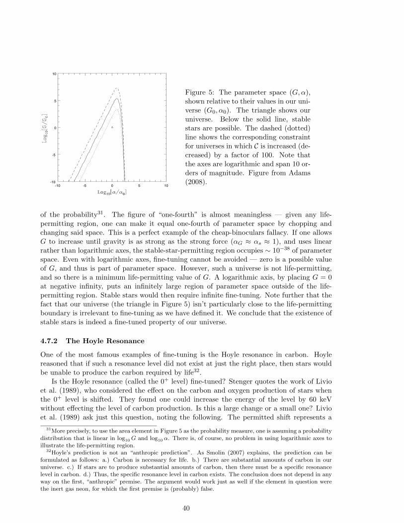
The Fine-Tuning of the Universe for Intelligent Life Luke A. Barnes Institute for Astronomy ETH Zurich Switzerland Sydney Institute for Astronomy School of Physics University of Sydney Australia June 11, 2012 Abstract The fine-tuning of the universe for intelligent life has received a great deal of attention in recent years, both in the philosophical and scientific literature. The claim is that in the space of possible physical laws, parameters and initial conditions, the set that permits the evolution of intelligent life is very small. I present here a review of the scientific literature, outlining cases of fine-tuning in the classic works of Carter, Carr and Rees, and Barrow and Tipler, as well as more recent work. To sharpen the discussion, the role of the antagonist will be played by Victor Stenger’s recent book The Fallacy of Fine-Tuning: Why the Universe is Not Designed for Us. Stenger claims that all known fine-tuning cases can be explained without the need for a multiverse. Many of Stenger’s claims will be found to be highly problematic. We will touch on such issues as the logical necessity of the laws of nature; objectivity, invariance and symmetry; theoretical physics and possible universes; entropy in cosmology; cosmic inflation and initial conditions; galaxy formation; the cosmological constant; stars and their formation; the properties of elementary particles and their effect on chemistry and the macroscopic world; the origin of mass; grand unified theories; and the dimensionality of space and time. I also provide an assessment of the multiverse, noting the significant challenges that it must face. I do not attempt to defend any conclusion based on the fine-tuning of the universe for intelligent life. This paper can be viewed as a critique of Stenger’s book, or read independently. arXiv:1112.4647v2 [physics.hist-ph] 7 Jun 2012
Transcript
The Fine-Tuning of the Universe
for Intelligent Life
Luke A. Barnes
Institute for AstronomyETH ZurichSwitzerland
Sydney Institute for AstronomySchool of Physics
University of SydneyAustralia
June 11, 2012
Abstract
The fine-tuning of the universe for intelligent life has received a great deal of attention in recentyears, both in the philosophical and scientific literature. The claim is that in the space ofpossible physical laws, parameters and initial conditions, the set that permits the evolution ofintelligent life is very small. I present here a review of the scientific literature, outlining casesof fine-tuning in the classic works of Carter, Carr and Rees, and Barrow and Tipler, as wellas more recent work. To sharpen the discussion, the role of the antagonist will be played byVictor Stenger’s recent book The Fallacy of Fine-Tuning: Why the Universe is Not Designedfor Us. Stenger claims that all known fine-tuning cases can be explained without the needfor a multiverse. Many of Stenger’s claims will be found to be highly problematic. We willtouch on such issues as the logical necessity of the laws of nature; objectivity, invariance andsymmetry; theoretical physics and possible universes; entropy in cosmology; cosmic inflationand initial conditions; galaxy formation; the cosmological constant; stars and their formation;the properties of elementary particles and their effect on chemistry and the macroscopic world;the origin of mass; grand unified theories; and the dimensionality of space and time. I alsoprovide an assessment of the multiverse, noting the significant challenges that it must face. Ido not attempt to defend any conclusion based on the fine-tuning of the universe for intelligentlife. This paper can be viewed as a critique of Stenger’s book, or read independently.
The fine-tuning of the universe for intelligent life has received much attention in recent times.Beginning with the classic papers of Carter (1974) and Carr & Rees (1979), and the extensivediscussion of Barrow & Tipler (1986), a number of authors have noticed that very smallchanges in the laws, parameters and initial conditions of physics would result in a universeunable to evolve and support intelligent life.
We begin by defining our terms. We will refer to the laws of nature, initial conditions andphysical constants of a particular universe as its physics for short. Conversely, we define a
2
‘universe’ be a connected region of spacetime over which physics is effectively constant1. Theclaim that the universe is fine-tuned can be formulated as:
FT: In the set of possible physics, the subset that permit the evolution of life isvery small.
FT can be understood as a counterfactual claim, that is, a claim about what would havebeen. Such claims are not uncommon in everyday life. For example, we can formulate theclaim that Roger Federer would almost certainly defeat me in a game of tennis as: “in theset of possible games of tennis between myself and Roger Federer, the set in which I win isextremely small”. This claim is undoubtedly true, even though none of the infinitely-manypossible games has been played.
Our formulation of FT, however, is in obvious need of refinement. What determines theset of possible physics? Where exactly do we draw the line between “universes”? How is“smallness” being measured? Are we considering only cases where the evolution of life isphysically impossible or just extremely improbable? What is life? We will press on with theour formulation of FT as it stands, pausing to note its inadequacies when appropriate. As itstands, FT is precise enough to distinguish itself from a number of other claims for which itis often mistaken. FT is not the claim that this universe is optimal for life, that it containsthe maximum amount of life per unit volume or per baryon, that carbon-based life is the onlypossible type of life, or that the only kinds of universes that support life are minor variationson this universe. These claims, true or false, are simply beside the point.
The reason why FT is an interesting claim is that it makes the existence of life in thisuniverse appear to be something remarkable, something in need of explanation. The intuitionhere is that, if ours were the only universe, and if the causes that established the physics ofour universe were indifferent to whether it would evolve life, then the chances of hitting upona life-permitting universe are very small. As Leslie (1989, pg. 121) notes, “[a] chief reasonfor thinking that something stands in special need of explanation is that we actually glimpsesome tidy way in which it might be explained”. Consider the following tidy explanations:
• This universe is one of a large number of variegated universes, produced by physicalprocesses that randomly scan through (a subset of) the set of possible physics. Even-tually, a universe will be created that is a member of the life-permitting set. Only suchuniverses can be observed, since only such universes contain observers.
• There exists a transcendent, personal creator of the universe. This entity desires tocreate a universe in which other minds will be able to form. Thus, the entity choosesfrom the set of possibilities a universe which is foreseen to evolve intelligent life2.
These scenarios are neither mutually exclusive nor exhaustive, but if either or both were truethen we would have a tidy explanation of why our universe, against the odds, supports theevolution of life.
Our discussion of the multiverse will touch on the so-called anthropic principle, which wewill formulate as follows:
1We may wish to stipulate that a given observer by definition only observes one universe. Such finer pointswill not effect our discussion
2The counter-argument presented in Stenger’s book (page 252), borrowing from a paper by Ikeda andJeffreys, does not address this possibility. Rather, it argues against a deity which intervenes to sustain life inthis universe. I have discussed this elsewhere: ikedajeff.notlong.com
3
AP: If observers observe anything, they will observe conditions that permit theexistence of observers.
Tautological? Yes! The anthropic principle is best thought of as a selection effect. Selectioneffects occur whenever we observe a non-random sample of an underlying population. Sucheffects are well known to astronomers. An example is Malmquist bias — in any survey ofthe distant universe, we will only observe objects that are bright enough to be detected byour telescope. This statement is tautological, but is nevertheless non-trivial. The penalty ofignoring Malmquist bias is a plague of spurious correlations. For example, it will seem thatdistant galaxies are on average intrinsically brighter than nearby ones.
A selection bias alone cannot explain anything. Consider the case of quasars. When firstdiscovered, quasars were thought to be a strange new kind of star in our galaxy. Schmidt(1963) measured their redshift, showing that they were more than a million times furtheraway than previously thought. It follows that they must be incredibly bright. The questionthat naturally arises is: how are quasars so luminous? The (best) answer is: because quasarsare powered by gravitational energy released by matter falling into a super-massive black hole(Zel’dovich, 1964; Lynden-Bell, 1969). The answer is not: because otherwise we wouldn’t seethem. Noting that if we observe any object in the very distant universe then it must bevery bright does not explain why we observe any distant objects at all. Similarly, AP cannotexplain why life and its necessary conditions exist at all.
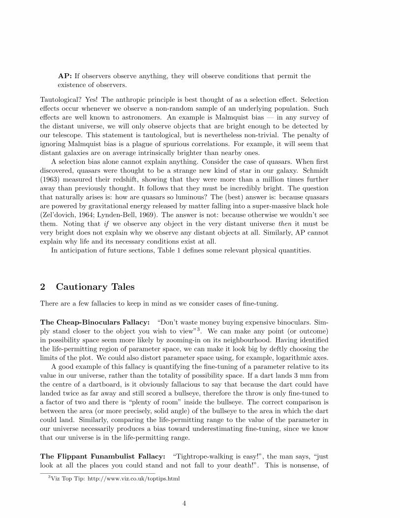
In anticipation of future sections, Table 1 defines some relevant physical quantities.
2 Cautionary Tales
There are a few fallacies to keep in mind as we consider cases of fine-tuning.
The Cheap-Binoculars Fallacy: “Don’t waste money buying expensive binoculars. Sim-ply stand closer to the object you wish to view”3. We can make any point (or outcome)in possibility space seem more likely by zooming-in on its neighbourhood. Having identifiedthe life-permitting region of parameter space, we can make it look big by deftly choosing thelimits of the plot. We could also distort parameter space using, for example, logarithmic axes.
A good example of this fallacy is quantifying the fine-tuning of a parameter relative to itsvalue in our universe, rather than the totality of possibility space. If a dart lands 3 mm fromthe centre of a dartboard, is it obviously fallacious to say that because the dart could havelanded twice as far away and still scored a bullseye, therefore the throw is only fine-tuned toa factor of two and there is “plenty of room” inside the bullseye. The correct comparison isbetween the area (or more precisely, solid angle) of the bullseye to the area in which the dartcould land. Similarly, comparing the life-permitting range to the value of the parameter inour universe necessarily produces a bias toward underestimating fine-tuning, since we knowthat our universe is in the life-permitting range.
The Flippant Funambulist Fallacy: “Tightrope-walking is easy!”, the man says, “justlook at all the places you could stand and not fall to your death!”. This is nonsense, of
(Reduced) Planck constant ~ 1.05457148 ×10⁻³⁴ m2 kg s−2
Planck mass-energy mPl =√~c/G 1.2209 ×10²² MeV
Mass of electron; proton; neutron me; mp; mn 0.511; 938.3; 939.6 MeVMass of up; down; strange quark mu; md; ms (Approx.) 2.4; 4.8; 104 MeVRatio of electron to proton mass β (1836.15)−1
Total matter mass per photon ξ ≈ 4 eVBaryonic mass per photon ξbaryon ≈ 0.61 eV
Table 1: Fundamental and derived physical and cosmological parameters, using the definitionsin Burgess & Moore (2006). Many of these quantities are listed in Tegmark et al. (2006),Burgess & Moore (2006, Table A.2) and Nakamura (2010). Unless otherwise noted, standardmodel coupling constants are evaluated at mZ , the mass of the Z particle, and hereafter wewill use Planck units: G = ~ = c = 1, unless reintroduced for clarity. Note that often in thefine-tuning literature (e.g. Carr & Rees, 1979; Barrow & Tipler, 1986, pg. 354), the low energyweak coupling constant is defined as αw ≡ GFm
2e , where GF = 1/
√2v2 = (292.8 GeV)−2 is
the Fermi constant. Using the definition of the Yukawa coupling above, we can write this asαw = Γ2
e/2√
2 ≈ 3× 10⁻¹². Note that this means that αw is independent of α2.
5
course: a tightrope walker must overbalance in a very specific direction if her path is to belife-permitting. The freedom to wander is tightly constrained. When identifying the life-permitting region of parameter space, the shape of the region is not particularly relevant. Anelongated life-friendly region is just as fine-tuned as a compact region of the same area. Thefact that we can change the setting on one cosmic dial, so long as we very carefully changeanother at the same time, does not necessarily mean that FT is false.
The Sequential Juggler Fallacy: “Juggling is easy!”, the man says, “you can throw andcatch a ball. So just juggle all five, one at a time”. Juggling five balls one-at-a-time isn’treally juggling. For a universe to be life-permitting, it must satisfy a number of constraintssimultaneously. For example, a universe with the right physical laws for complex organicmolecules, but which recollapses before it is cool enough to permit neutral atoms will notform life. One cannot refute FT by considering life-permitting criteria one-at-a-time andnoting that each can be satisfied in a wide region of parameter space. In set-theoretic terms,we are interested in the intersection of the life-permitting regions, not the union.
The Cane Toad Solution: In 1935, the Bureau of Sugar Experiment Stations was worriedby the effect of the native cane beetle on Australian sugar cane crops. They introduced 102cane toads, imported from Hawaii, into parts of Northern Queensland in the hope that theywould eat the beetles. And thus the problem was solved forever, except for the 200 millioncane toads that now call eastern Australia home, eating smaller native animals, and secretinga poison that kills any larger animal that preys on them. A cane toad solution, then, is onethat doesn’t consider whether the end result is worse than the problem itself. When presentedwith a proposed fine-tuning explainer, we must ask whether the solution is more fine-tunedthan the problem.
3 Stenger’s Case
We will sharpen the presentation of cases of fine-tuning by responding to the claims of VictorStenger. Stenger is a particle physicist, a noted speaker, and the author of a number of booksand articles on science and religion. In his latest book, “The Fallacy of Fine-Tuning: Whythe Universe is Not Designed for Us”4, he makes the following bold claim:
“[T]he most commonly cited examples of apparent fine-tuning can be readilyexplained by the application of a little well-established physics and cosmology.. . . [S]ome form of life would have occurred in most universes that could be de-scribed by the same physical models as ours, with parameters whose ranges variedover ranges consistent with those models. And I will show why we can expect tobe able to describe any uncreated universe with the same models and laws withat most slight, accidental variations. Plausible natural explanations can be foundfor those parameters that are most crucial for life. . . . My case against fine-tuningwill not rely on speculations beyond well-established physics nor on the existenceof multiple universes.” [Foft 22, 24]
Let’s be clear on the task that Stenger has set for himself. There are a great manyscientists, of varying religious persuasions, who accept that the universe is fine-tuned for
4Hereafter, “Foft x” will refer to page x of Stenger’s book.
6
life, e.g. Barrow, Carr, Carter, Davies, Dawkins, Deutsch, Ellis, Greene, Guth, Harrison,Hawking, Linde, Page, Penrose, Polkinghorne, Rees, Sandage, Smolin, Susskind, Tegmark,Tipler, Vilenkin, Weinberg, Wheeler, Wilczek5. They differ, of course, on what conclusionwe should draw from this fact. Stenger, on the other hand, claims that the universe is notfine-tuned.
4 Cases of Fine-Tuning
What is the evidence that FT is true? We would like to have meticulously examined everypossible universe and determined whether any form of life evolves. Sadly, this is currentlybeyond our abilities. Instead, we rely on simplified models and more general arguments tostep out into possible-physics-space. If the set of life-permitting universes is small amongstthe universes that we have been able to explore, then we can reasonably infer that it is unlikelythat the trend will be miraculously reversed just beyond the horizon of our knowledge.
4.1 The Laws of Nature
Are the laws of nature themselves fine-tuned? Stenger defends the ambitious claim that thelaws of nature could not have been different because they can be derived from the requirementthat they be Point-of-View Invariant (hereafter, PoVI). He says:
“. . . [In previous sections] we have derived all of classical physics, including classicalmechanics, Newton’s law of gravity, and Maxwell’s equations of electromagnetism,from just one simple principle: the models of physics cannot depend on the pointof view of the observer. We have also seen that special and general relativity followfrom the same principle, although Einstein’s specific model for general relativitydepends on one or two additional assumptions. I have offered a glimpse at howquantum mechanics also arises from the same principle, although again a few otherassumptions, such as the probability interpretation of the state vector, must beadded. . . . [The laws of nature] will be the same in any universe where no specialpoint of view is present.” [Foft 88, 91]
4.1.1 Invariance, Covariance and Symmetry
We can formulate Stenger’s argument for this conclusion as follows:
LN1. If our formulation of the laws of nature is to be objective, it must be PoVI.
LN3. Thus, “when our models do not depend on a particular point or direction in space or aparticular moment in time, then those models must necessarily contain the quantitieslinear momentum, angular momentum, and energy, all of which are conserved. Physi-cists have no choice in the matter, or else their models will be subjective, that is, willgive uselessly different results for every different point of view. And so the conservation
5References: Barrow & Tipler (1986), Carr & Rees (1979), Carter (1974), Davies (2006), Dawkins (2006),Redfern (2006) for Deutsch’s view on fine-tuning, Ellis (1993), Greene (2011), Guth (2007), Harrison (2003),Hawking & Mlodinow (2010, pg. 161), Linde (2008), Page (2011b), Penrose (2004, pg. 758), Polkinghorne &Beale (2009), Rees (1999), Smolin (2007), Susskind (2005), Tegmark et al. (2006), Vilenkin (2006), Weinberg(1994) and Wheeler (1996). See also Carr (2007).
7
principles are not laws built into the universe or handed down by deity to govern thebehavior of matter. They are principles governing the behavior of physicists.” [Foft82, emphasis original]
This argument commits the fallacy of equivocation — the term “invariant” has changed itsmeaning between LN1 and LN2. The difference is decisive but rather subtle, owing to thedifferent contexts in which the term can be used. We will tease the two meanings apart bydefining covariance and symmetry, considering a number of test cases.
Galileo’s Ship: We can see where Stenger’s argument has gone wrong with a simple ex-ample, before discussing technicalities in later sections. Consider this delightful passage fromGalileo regarding the brand of relativity that bears his name:
“Shut yourself up with some friend in the main cabin below decks on some largeship, and have with you there some flies, butterflies, and other small flying animals.Have a large bowl of water with some fish in it; hang up a bottle that emptiesdrop by drop into a wide vessel beneath it. With the ship standing still, observecarefully how the little animals fly with equal speed to all sides of the cabin. Thefish swim indifferently in all directions; the drops fall into the vessel beneath;and, in throwing something to your friend, you need throw it no more stronglyin one direction than another, the distances being equal; jumping with your feettogether, you pass equal spaces in every direction. When you have observed allthese things carefully (though doubtless when the ship is standing still everythingmust happen in this way), have the ship proceed with any speed you like, so longas the motion is uniform and not fluctuating this way and that. You will discovernot the least change in all the effects named, nor could you tell from any of themwhether the ship was moving or standing still6.”
Note carefully what Galileo is not saying. He is not saying that the situation can be viewedfrom a variety of different viewpoints and it looks the same. He is not saying that we candescribe flight-paths of the butterflies using a coordinate system with any origin, orientationor velocity relative to the ship.
Rather, Galileo’s observation is much more remarkable. He is stating that the two sit-uations, the stationary ship and moving ship, which are externally distinct are neverthelessinternally indistinguishable. We will borrow a definition from Healey (2007, Chapter 6):
“A 1-1 mapping φ : S → S of a set of situations onto itself is a strong empiricalsymmetry if and only if no two situations related by φ can be distinguished bymeans of measurements confined to each situation.”
Galileo is saying that situations that are moving at a constant velocity with respect to eachother are related by a strong empirical symmetry. There are two situations, not one. Theseare not different descriptions of the same situation, but rather different situations with thesame internal properties.
The reason why Galilean relativity is so shocking and counterintuitive7 is that there is noa priori reason to expect distinct situations to be indistinguishable. If you and your friend
6Quoted in Healey (2007, Chapter 6).7It remains so today, as evidenced by the difficulty that even good lecturers have in successfully teaching
Newtonian mechanics to undergraduates (Griffiths, 1997).
8
attempt to describe the butterfly in the stationary ship and end up with “uselessly differentresults”, then at least one of you has messed up your sums. If your friend tells you his point-of-view, you should be able to perform a mathematical transformation on your model andreproduce his model. None of this will tell you how the butterflies will fly when the ship isspeeding on the open ocean. An Aristotelian butterfly would presumably be plastered againstthe aft wall of the cabin. It would not be heard to cry: “Oh, the subjectivity of it all!”
Galilean relativity, and symmetries in general, have nothing whatsoever to do with point-of-view invariance. A universe in which Galilean relativity did not hold would not wallowin subjectivity. It would be an objective, observable fact that the butterflies would fly dif-ferently in a speeding ship. This is Stenger’s confusion: requiring objectivity in describing agiven situation does not imply a symmetry. Symmetries relate distinct-but-indistinguishablesituations.
Lagrangian Dynamics: We can see this same point in a more formal context. Lagrangiandynamics is a framework for physical theories that, while originally developed as a powerfulapproach to Newtonian dynamics, underlies much of modern physics. Relativity, quantumfield theory and even string theory can be (and often are) formulated in terms of Lagrangians.Without loss of generality, we will consider here classical Lagrangian dynamics. The methodof analysing a physical system in Lagrangian dynamics is as follows:
• Write down coordinates (qi) representing each of the degrees of freedom of your system.For example, for two beads moving along a wire, q1 can represent the position of particle1, and q2 for particle 2.
• Write down the Lagrangian (L) (classically, the kinetic minus potential energy) of thesystem in terms of time t, the coordinates qi, and their time derivatives qi.
• The equations governing how the qi change with time are found by minimising the‘action’: S =
∫Ldt. Through the wonders of calculus of variations, this is equivalent
to solving the Euler-Lagrange equation,
d
dt
(∂L
∂qi
)− ∂L
∂qi= 0 . (1)
One of the features of the Lagrangian formalism is that it is covariant. Suppose that wereturn to the first step and decide that we want to use different coordinates for our system,say si, which are expressed as functions of the old coordinates qi and t. We can then expressthe Lagrangian L in terms of t, si and si by substituting the new coordinates for the oldones. Now, what equation must we solve to minimise the action? The answer is equation1 again, but replacing q’s with s’s. In other words, it does not matter what coordinates weuse. The equations take the same form in any coordinate system, and are thus said to becovariant. Note that this is true of any Lagrangian, and any (sufficiently smooth) coordinatetransformation si(t, qj). Objectivity (and PoVI) are guaranteed.
Now, consider a specific Lagrangian L that has the following special property — thereexists a continuous family of coordinate transformations that leave L unchanged. Such atransformation is called a symmetry (or isometry) of the Lagrangian. The simplest case iswhere a particular coordinate does not appear in the expression for L. Noether’s theoremtells us that, for each continuous symmetry, there will be a conserved quantity. For example,if time does not appear explicitly in the Lagrangian, then energy will be conserved.
9
Note carefully the difference between covariance and symmetry. Both could justifiablybe called “coordinate invariance” but they are not the same thing. Covariance is a propertyof the entire Lagrangian formalism. A symmetry is a property of a particular LagrangianL. Covariance holds with respect to all (sufficiently smooth) coordinate transformations.A symmetry is linked to a particular coordinate transformation. Covariance gives us noinformation whatsoever about which Lagrangian best describes a given physical scenario.Symmetries provide strong constraints on the which Lagrangians are consistent with empiricaldata. Covariance is a mathematical fact about our formalism. Symmetries can be confirmedor falsified by experiment.
Furthermore, Noether’s theorem only links symmetry to conservation for particles andfields that obey the principle of least action. As Brading and Brown (in Brading & Castellani,2003, pg. 99) note:
“. . . in order to make the connection between a certain symmetry and an associ-ated conservation law, we must . . . involve dynamically significant information orassumptions, such as the assumption that all the fields in the theory satisfy theEuler-Lagrange equations of motion. . . . Thus, when we use Noether’s first theo-rem to connect a symmetry with a conservation law we have to put the relevantdynamical information.”
The principle of least action is not a necessary truth; neither does it follow from PoVI.Finally, the Lagrangian formalism itself is not forced upon us a priori. There are plenty ofother mathematical structures and systems lurking in the set of all possible worlds.
Symmetry and Mere Redescription: It will be useful to clarify how a theory can give“uselessly different results”. When a theoretical calculation predicts an observation, it isobviously unacceptable for the theory to give multiple answers when observation gives one.Consider, for example, describing the motion of the Earth and Sun in Newtonian mechanics.We introduce a coordinate system representing the position of each body as an element(x, y, z) ∈ R3. Calculating the period of the Earth’s orbit must not depend on our choiceof mathematical apparatus introduced to aid calculation. Changing the coordinate systemis mere redescription; the Earth in any coordinate system will still complete its orbit in365.256363 days.
Here is the crucial point: the fact that we are free to describe the system in a rotatedcoordinate system neither implies nor follows from the rotational symmetry of the system.Suppose that Newton’s law of gravitation were modified by a dipole-like term,
F = −G m1m2
|r12|2r12 (1 + αd r12 · b) , (2)
where a hatted vector is of unit length, r12 = r1− r2, αd is a dimensionless parameter, and bis a fixed unit vector. Due to the term involving b, this law is not rotationally symmetric, andthus angular momentum is not conserved. However, we are still free to use any coordinatesystem to describe they system. In particular, we are free use a Cartesian coordinate systemrotated to any orientation and our prediction of the outcome of any observation will remainthe same.
Lorentz Invariance: Let’s look more closely at some specific cases. Stenger applies hisgeneral PoVI argument to Einstein’s special theory of relativity:
10
“Special relativity similarly results from the principle that the models of physicsmust be the same for two observers moving at a constant velocity with respect toone another. . . . Physicists are forced to make their models Lorentz invariant sothey do not depend on the particular point of view of one reference frame movingwith respect to another.”
This claim is false. Physicists are perfectly free to postulate theories which are not Lorentzinvariant, and a great deal of experimental and theoretical effort has been expended to thisend. The compilation of Kostelecky & Russell (2011) cites 127 papers that investigate Lorentzviolation. Pospelov & Romalis (2004) give an excellent overview of this industry, giving anexample of a Lorentz-violating Lagrangian:
L = −bµψγµγ5ψ −1
2Hµνψσ
µνψ − kµεµναβAνAβ,α , (3)
where the fields bµ, kµ and Hµν are external vector and antisymmetric tensor backgroundsthat introduce a preferred frame and therefore break Lorentz invariance; all other symbolshave their usual meanings (e.g. Nagashima, 2010). A wide array of laboratory, astrophysicaland cosmological tests place impressively tight bounds on these fields. At the moment Lorentzinvariance is just a theoretical possibility. But that’s the point.
Take the work of Bear et al. (2000), who attempt to measure bµ using a spin maserexperiment. If Stenger were correct, this experiment would be aimed at finding objectiveevidence that physics is subjective. Thankfully, they report that the objectivity of physicshas been confirmed to a level of 10−31 GeV. Future experiments may provide convincing,reproducible, empirical evidence that physicists might as well give up.
Ironically, the best cure to Stenger’s conflation of “frame-dependent” with “subjective” isspecial relativity. The length of a rigid rod depends on the reference frame of the observer: if itis 2 metres long it its own rest frame, it will be 1 metre long in the frame of an observer passingat 87% of the speed of light8. It does not follow that the length of the rod is “subjective”,in the sense that the length of the rod is just the personal opinion of a given observer, orin the sense that these two different answers are “uselessly different”. It is an objectivefact that the length of the rod is frame-dependent. Physics is perfectly capable of studyingframe-dependent quantities, like the length of a rod, and frame-dependent laws, such as theLagrangian in Equation 3.
We can look at the “axioms” of special relativity and see whether these must hold in allpossible universes. Einstein famously proposed two postulates: the principle of relativity, thatall inertial frames are totally equivalent for the performance of all physical experiments (cf.Rindler, 2006), and the constancy of the speed of light in every inertial frame. One must alsoassume spacetime homogeneity and spatial isotropy in order to derive the Lorentz transform9.
Which of these axioms are necessarily true? None. The relativity principle isn’t evenobviously true, as the two millennia between Aristotle and Galileo demonstrate, and Galileo(and Newton) only applied the principle to mechanics; Einstein extended the principle to
8Note that it isn’t just that the rod appears to be shorter. Length contraction in special relativity is notjust an optical illusion resulting from the finite speed of light. See, for example, Penrose (1959).
9Beginning with von Ignatowsky (1910), many have attempted to derive the Lorentz transform withoutEinstein’s second postulate (see Field, 2004; Rindler, 2006; Certik, 2007, and references therein); John Stewart’s(unpublished) lecture notes inform us that: “This derivation . . . has be re-invented approximately once a decadeby physicists believing their research to be original (present author not excepted)”. Such derivations involveadditional assumptions, most commonly that the Lorentz transformations form a group.
11
all possible physical experiments. The problem with “Aristotle’s second law” — all bodiespersist in their state of rest unless acted on by an external force (Wigner, as quoted in Brading& Castellani, 2003, pg. 368) — is not that there is a lurking contradiction, nor is it that auniverse which obeyed such a law would be tossed to and fro by every physicist whim. Theproblem is that it’s empirically false. The second postulate certainly isn’t necessary — there isnothing logically contradictory about a universe that respects Galilean invariance. Similarly,the Lagrangian in Equation (3) shows that we can formulate physical theories which do notrespect translational and rotational symmetry. As Wigner warns, “Einstein’s work establishedthe [principles underlying special relativity] so firmly that we have to be reminded that theyare based only on experience”.
General Relativity: We turn now to Stenger’s discussion of gravity.
“Ask yourself this: If the gravitational force can be transformed away by go-ing to a different reference frame, how can it be “real”? It can’t. We see thatthe gravitational force is an artifact, a “fictitious” force just like the centrifugaland Coriolis forces . . . [If there were no gravity] then there would be no universe. . . [P]hysicists have to put gravity into any model of the universe that containsseparate masses. A universe with separated masses and no gravity would violatepoint-of-view invariance. . . . In general relativity, the gravitational force is treatedas a fictitious force like the centrifugal force, introduced into models to preserveinvariance between reference frames accelerating with respect to one another.”
These claims are mistaken. The existence of gravity is not implied by the existence of theuniverse, separate masses or accelerating frames.
Stenger’s view may be rooted in the rather persistent myth that special relativity cannothandle accelerating objects or frames, and so general relativity (and thus gravity) is required.The best remedy to this view is some extra homework: sit down with the excellent textbook ofHartle (2003) and don’t get up until you’ve finished Chapter 5’s “systematic way of extractingthe predictions for observers who are not associated with global inertial frames . . . in thecontext of special relativity”. Special relativity is perfectly able to preserve invariance betweenreference frames accelerating with respect to one another. Physicists clearly don’t have toput gravity into any model of the universe that contains separate masses.
We can see this another way. None of the invariant/covariant properties of general rela-tivity depend on the value of Newton’s constant G. In particular, we can set G = 0. In sucha universe, the geometry of spacetime would not be coupled to its matter-energy content,and Einstein’s equation would read Rµν = 0. With no source term, local Lorentz invarianceholds globally, giving the Minkowski metric of special relativity. Neither logical necessity norPoVI demands the coupling of spacetime geometry to mass-energy. This G = 0 universe is acounterexample to Stenger’s assertion that no gravity means no universe.
What of Stenger’s claim that general relativity is merely a fictitious force, to can be derivedfrom PoVI and “one or two additional assumptions”? Interpreting PoVI as what Einsteincalled general covariance, PoVI tells us almost nothing. General relativity is not the onlycovariant theory of spacetime (Norton, 1995). As Misner et al. (1973, pg. 302) note: “Anyphysical theory originally written in a special coordinate system can be recast in geometric,coordinate-free language. Newtonian theory is a good example, with its equivalent geometricand standard formulations. Hence, as a sieve for separating viable theories from nonviable
12
theories, the principle of general covariance is useless.” Similarly, Carroll (2003) tells us thatthe principle “Laws of physics should be expressed (or at least be expressible) in generallycovariant form” is “vacuous”.
Suppose that, feeling generous, we allow Stenger to assume the equivalence principle10,which is what he is referring to when he calls gravity a ‘fictitious force’. The problem isthat the equivalence principle applies to a limiting case: a freely falling frame, infinitesimallysmall, observed for an infinitesimally short period of time. The most we can infer/guess fromthis is that there exists a metric on spacetime which is locally Minkowskian, the curvatureof which we interpret as gravity, as well as the requirement that the coupling of matter tocurvature does not allow curvature to be measured locally (Carroll, 2003). This inference isbest described as a well-motivated suggestion rather than a rigorously derived consequence.
Now, how far are we from Einstein’s field equation? The most common next step in thederivation is to turn our attention to the aspects of gravity which cannot be transformedaway, which are not fictitious11. Two observers falling toward the centre of the Earth inside alift will be able to distinguish their state of motion from that in an empty universe by the factthat their paths are converging. Something appears to be pushing them together – a tidalfield. It follows that the presence of a genuine gravitation field, as opposed to an inertial field,can be verified by the variation of the field. From this starting point, via a generalisationof the equation of geodesic deviation from Newtonian gravity, we link the real, non-fictitiousproperties of the gravitational field to Riemann tensor and its contractions. In this respect,gravity is not a fictional force in the same sense that the centrifugal force is. We can alwaysremove the centrifugal force everywhere by transforming to an inertial frame. This cannot bedone for gravity.
We can now identify the “additional assumptions” that Stenger needs to derive generalrelativity. Given general covariance (or PoVI), the additional assumptions constitute theentire empirical content of the theory. Even if we assume the equivalence principle, weneed additional information about what the gravitational properties of matter actually do tospacetime. These are the dynamic principles of spacetime, the very reasons why Einstein’stheory can be called geometrodynamics. Stenger’s attempts to trivialise gravity thus fail. Weare free to consider the fine-tuning of gravity, both its existence and properties.
Finally, general relativity provides a perfect counterexample to Stenger’s conflation ofcovariance with symmetry. Einstein’s GR field equation is covariant — it takes the sameform in any coordinate system, and applying a coordinate transformation to a particularsolution of the GR equation yields another solution, both representing the same physicalscenario. Thus, any solution of the GR equation is covariant, or PoVI. But it does not follow
10This is generosity indeed. The fact that the two cannonballs dropped (probably apocryphally) off theTower of Pisa by Galileo hit the ground at the same time is certainly not a necessary truth; neither doesfollow from PoVI. This is an equivalence between two different experiments, not two different viewpoints. Aswith Lorentz violation, considerable theoretical and observational effort has been expended in formulating andtesting equivalence-principle-violating theories (Uzan, 2011), guided by the realisation that ‘[d]espite its name,the “Equivalence Principle” (EP) is not one of the basic principles of physics. There is nothing taboo abouthaving an observational violation of the EP’ (Damour, 2009).
11For example, Hartle (2003); D’Inverno (2004) take this approach via the Newtonian equation of geodesicdeviation. Wald (1984); Carroll (2003); Hobson et al. (2005); Rindler (2006) take a shortcut by guessing theform of the Einstein equation from the (Newtonian) Poisson equation. Misner et al. (1973) present six sets ofaxioms from which to derive Einstein’s equation, together with the warning that “[b]y now the equation tellswhat axioms are acceptable”. Most of these books also derive the equation from a variational principle, whichrelies heavily on simplicity as a guiding principle. In fact, the variational approach is the best way to explorethe “uncountable number” of ways in which general relativity could be modified (Carroll, 2003, pg. 181).
13
that a particular solution will exhibit any symmetries. There may be no conserved quantitiesat all. As Hartle (2003, pg. 176, 342) explains:
“Conserved quantities . . . cannot be expected in a general spacetime that has nospecial symmetries . . . The conserved energy and angular momentum of particleorbits in the Schwarzschild geometry12 followed directly from its time displacementand rotational symmetries. . . . But general relativity does not assume a fixedspacetime geometry. It is a theory of spacetime geometry, and there are nosymmetries that characterize all spacetimes.”
The Standard Model of Particle Physics and Gauge Invariance: We turn now toparticle physics, and particularly the gauge principle. Interpreting gauge invariance as “justa fancy technical term for point-of-view invariance” [Foft 86], Stenger says:
“If [the phase of the wavefunction] is allowed to vary from point to point in space-time, Schrodinger’s time-dependent equation . . . is not gauge invariant. However,if you insert a four-vector field into the equation and ask what that field has tobe to make everything nice and gauge invariant, that field is precisely the four-vector potential that leads to Maxwell’s equations of electromagnetism! That is,the electromagnetic force turns out to be a fictitious force, like gravity, introducedto preserve the point-of-view invariance of the system. . . . Much of the standardmodel of elementary particles also follows from the principle of gauge invariance.”[Foft 86-88]
Remember the point that Stenger is trying to make: the laws of nature are the same in anyuniverse which is point-of-view invariant.
Stenger’s discussion glosses over the major conceptual leap from global to local gaugeinvariance. Most discussions of the gauge principle are rather cautious at this point. Yang,who along with Mills first used the gauge principle as a postulate in a physical theory, com-mented that “We did not know how to make the theory fit experiment. It was our judgement,however, that the beauty of the idea alone merited attention”. Kaku (1993, pg. 11), whoprovides this quote, says of the argument for local gauge invariance:
“If the predictions of gauge theory disagreed with the experimental data, then onewould have to abandon them, no matter how elegant or aesthetically satisfyingthey were. Gauge theorists realized that the ultimate judge of any theory wasexperiment.”
Similarly, Griffiths (2008) “knows of no compelling physical argument for insisting that globalinvariance should hold locally” [emphasis original]. Aitchison & Hey (2002) says that this lineof thought is “not compelling motivation” for the step from global to local gauge invariance,and along with Pokorski (2000), who describes the argument as aesthetic, ultimately appealsto the empirical success of the principle for justification. Needless to say, these are not theviews of physicists demanding that all possible universes must obey a certain principle13.
12That is, the spacetime of a non-rotating, uncharged black hole.13See also the excellent articles by Martin and Earman in Brading & Castellani (2003). Earman, in particular,
notes that the ‘gauge principle’ is viewed by Wald and Weinberg (et al.) as a consequence of other principles,i.e. output rather than input.
14
The argument most often advanced to justify local gauge invariance is that ‘local’ symme-tries are more in line with the locality of special relativity (i.e. no faster-than-light propagationof physical causes), in that we are letting each spacetime point choose its own phase conven-tion. This argument, however, seems to contradict itself. We begin by postulating that thephase of the wavefunction is unobservable, from which follows global gauge invariance. Theidea that all spacetime points adopt the same phase convention seems contrary to locality.This leads us to local gauge invariance. But the phase of the wavefunction isn’t a physicalcause. By hypothesis, the physical universe knows nothing of the phase of the wavefunction.The very reason for global gauge invariance seems to suggest that nature needn’t be botheredby local gauge invariance.
Secondly, we note again the difference between symmetry and PoVI. A universe describedby a Lagrangian that is not locally gauge invariant is not doomed to subjectivity. Stengernotes that the Lagrangian for a free charged particle is not invariant under a local gaugetransformation — e.g. the Dirac field: L = ψ(iγµ∂µ − m)ψ. If Stenger’s claims were cor-rect, one should be able to make “uselessly different” predictions from this Lagrangian usingnothing more than a relabelling of state space. We know, however that this cannot be donebecause of the covariance of the Lagrangian formalism. Coordinate invariance is guaranteedfor any Lagrangian (that obeys the action principle), locally gauge invariant or not. This isespecially true of the phase of the wavefunction because it is unobservable in principle.
Thirdly, a technicality regarding local gauge invariance in QED. The relevant Lagrangianis:
LQED = ψ(iγµ∂µ −m)ψ − qψγµψAµ −1
4FµνF
µν (4)
The gauge argument starts with the first term on the right hand side, the Dirac field for afree electron. Noting that this term is not locally gauge invariant, we ask what term mustbe added in order to restore invariance. We postulate that the second term is required,which is describes the interaction between the electron and a field, Aµ. Noting that thisfield has the same gauge properties as the electromagnetic field, we add the third term, theMaxwellian term. The term in Fµν ≡ ∂µAν − ∂νAµ gives the source-free Maxwell equationsof electromagnetism.
A few points need to be kept in mind. a.) The second term is not unique. There areinfinitely many other gauge invariant terms which could be added. The term shown above issingled out as being the simplest, renormalisable, Lorentz and gauge invariant term. Simplicityis not necessity. b.) Local gauge invariance does not demand that we add the third term. Itis consistent with local gauge invariance that Fµν ≡ 0, which implies a non-physical, formalcoupling of the matter field to trivial gauge fields (Brading & Castellani, 2003; Healey, 2007).By adding the third term, we have promoted the gauge field to a physical field by hand. This isa plausible step, a useful heuristic, but not a logical necessity. c.) Stenger claims that Dyson(1990) “provided a derivation of Maxwell’s equations from the Lorentz force law. . . . That is,Maxwell’s equations follow from the definition of the electric and magnetic fields”. Stengerfails to mention a few crucial details of the proof. Dyson assumes the following commutationrelations: [xj , xk] = 0, m[xj , xk] = i~δjk . These are the conditions for the classical systemto be quantizable, and are highly non-trivial. Hojman & Shepley (1991) shows that theseassumptions (plus Newton’s equation mx = Fj(x, x, t)) are equivalent to the Euler-Lagrangeequations of a Lagrangian L, and gives examples of classical equations that do not fulfil theseassumptions. Also, Dyson only proves two of Maxwell’s equations, assuming that the othertwo (∇ · E = 4πρ, -∂E/∂t + ∇ × B = 4πj) can be used to define the charge and current
15
density. As a number of authors (Anderson, 1991; Brehme, 1991; Dombey, 1991; Farquhar,1991; Vaidya, 1991) were quick to point out, this is also a non-trivial assumption. In particular,in response to the comment of Dyson (1990) that Galilean and Lorentz invariance seem to becoexisting peacefully in his derivation, it is noted that Lorentz invariance has been assumed inthe “definitions”. If Dyson had chosen different definitions of the charge and current density,he could have made the equations Galilean invariant. Alternatively, had Dyson replaced Ewith E/
√1− |E|2, then Coulomb’s law would not hold. Evidently, this is no mere change of
convention.Fourthly, we must ask: what else does a gauge theory need to postulate, other than local
gauge invariance? A gauge theory needs a symmetry group. Electromagnetism is based onU(1), the weak force SU(2), the strong force SU(3), and there are grand unified theories basedon SU(5), SO(10), E8 and more. These are just the theories with a chance of describing ouruniverse. From a theoretical point of view, there are any number of possible symmetries, e.g.SU(N) and SO(N) for any integer N (Schellekens, 2008). The gauge group of the standardmodel, SU(3)× SU(2)× U(1), is far from unique.
Finally, there is a deeper point that needs to be made about observable and unobserv-able quantities in physical theories. Our foray into gauge invariance was prompted by theunobservability of the phase of the wavefunction. This is not a mathematical fact about ourtheory. One cannot derive this fact from mathematical theorems about Hilbert space. It isan empirical fact, and a highly non-trivial one. It is the claim that there is no possible exper-iment, no observation of any kind anywhere in the universe that could measure the phase ofa wavefunction. Stenger’s casual observation that the probability interpretation of the statevector in quantum mechanics is an additional assumption [Foft 88] fails to acknowledgethe empirical significance of this postulate — this is the postulate underlying global gaugeinvariance, not PoVI. Here is Brading and Brown (in Brading & Castellani, 2003, pg. 99):
“The very fact that a global gauge transformation does not lead to empiricallydistinct predictions is itself non-trivial. In other words, the freedom in our de-scriptions is no ‘mere’ mathematical freedom — it is a consequence of a physicallysignificant structural feature of the theory. The same is true in the case of globalspacetime symmetries: the fact that the equations of motion are invariant undertranslations, for example, is empirically significant.” [Emphasis original.]
All physical theories must posit a correspondence between their mathematical apparatusand the physical world that they are attempting to describe. A good illustration of thispoint is the very first gauge theory. In 1918, Weyl considered the geometry that resultsfrom extending Einstein’s theory of general relativity by allowing arbitrary rescalings of thespacetime metric at each spacetime point14, coining the term ‘gauge’ symmetry for this kindof transformation. At the heart of Weyl’s idea was the assumption that the spacetime interval(ds2) was unobservable, and had no physical significance. While Weyl’s project showed somepromising signs — the gauge field could be identified with the electromagnetic field — Einsteinsoon pointed out its central flaw. The spacetime interval was observable, in the form ofspectral lines from atoms in distant stars and nebulae.
The moral of the story is simple but profound: the line that separates observable andunobservable in a physical theories is drawn by nature, not by us. The problem with Weyl’sfirst attempt at a gauge theory is not mathematical i.e. there is no internal inconsistency.
14My account here will follow Martin (in Brading & Castellani, 2003).
16
Neither is the problem one of subjectivity, or uselessly different predictions. The problem isthat the theory makes objective, point-of-view invariant predictions that are false.
Conclusion: We can now see the flaw in Stenger’s argument. Premise LN1 should read: Ifour formulation of the laws of nature is to be objective, then it must be covariant. PremiseLN2 should read: symmetries imply conserved quantities. Since ‘covariant’ and ‘symmetric’are not synonymous, it follows that the conclusion of the argument is unproven, and we wouldargue that it is false. The conservation principles of this universe are not merely principlesgoverning our formulation of the laws of nature. Neother’s theorems do not allow us to pullphysically significant conclusions out of a mathematical hat. If you want to know whethera certain symmetry holds in nature, you need a laboratory or a telescope, not a blackboard.Symmetries tell us something about the physical universe.
Some of our comments may seem to be nit-picking over mere technicalities. On the con-trary, those attempting the noble task of attacking Hilbert’s 6th problem — to find theaxioms of physics — will be disqualified if they are found to be smuggling secret assump-tions. Nitpicking and mere technicalities are the name of the game: Russell and Whitehead’sPrincipia Mathematica proved that “1 + 1 = 2” on page 86 of Volume II. Stenger’s extraor-dinary claim that only one axiom is needed — the near-trivial requirement that our theoriesdescribe an objective reality — dies the death of a thousand overlooked assumptions. Thefolly of Stenger’s account of modern physics is most clear in his claim to be able to deduceall of classical mechanics, Newton’s law of gravity, Maxwell’s equations of electromagnetism,special relativity, general relativity, quantum mechanics, and the standard model of particlephysics from one principle. These theories are based on contradictory principles, and makecontradictory predictions, reducing Stenger’s argument to ashes.
4.1.2 Is Symmetry Enough?
Suppose that Stenger were correct regarding symmetries, that any objective description ofthe universe must incorporate them. One of the features of the universe as we currentlyunderstand it is that it is not perfectly symmetric. Indeed, intelligent life requires a measureof asymmetry. For example, the perfect homogeneity and isotropy of the Robertson-Walkerspacetime precludes the possibility of any form of complexity, including life. Sakharov (1967)famously showed that for the universe to contain sufficient amounts of ordinary baryonicmatter, interactions in the early universe must violate baryon number conservation, charge-symmetry and charge-parity-symmetry, and must spend some time out of thermal equilibrium.Supersymmetry, too, must be a broken symmetry in any life-permitting universe, since thebosonic partner of the electron (the selectron) would make chemistry impossible (see thediscussion in Susskind, 2005, pg. 250). As Pierre Curie has said, it is asymmetry that createsa phenomena.
One of the most important concepts in modern physics is spontaneous symmetry breaking(SSB). As Strocchi (2007) explains, SSB forms the basis for recent achievements in statisticalmechanics, describes collective phenomena in solid state physics, and makes possible theunification of the weak, strong and electromagnetic forces of particle physics. The power ofSSB is precisely that it allows us
“. . . to understand how the conclusions of the Noether theorem can be evaded andhow a symmetry of the dynamics cannot be realized as a mapping of the physicalconfigurations of the system.” (Strocchi, 2007, pg. 3)
17
SSB allows the laws of nature to retain their symmetry and yet have asymmetric solutions.Even if the symmetries of the laws of nature were inevitable, it would still be an open questionas to precisely which symmetries were broken in our universe and which were unbroken.
4.1.3 Changing the Laws of Nature
What if the laws of nature were different? Stenger says:
“. . . what about a universe with a different set of “laws”? There is not much wecan say about such a universe, nor do we need to. Not knowing what any of theirparameters are, no one can claim that they are fine-tuned.” [Foft 69]
In reply, fine-tuning isn’t about what the parameters and laws are in a particular universe.Given some other set of laws, we ask: if a universe were chosen at random from the setof universes with those laws, what is the probability that it would support intelligent life?If that probability is suitably (and robustly) small, then we conclude that that region ofpossible-physics-space contributes negligibly to the total life-permitting subset. It is easy tofind examples of such claims.
• A universe governed by Maxwell’s Laws “all the way down” (i.e. with no quantumregime at small scales) will not have stable atoms — electrons radiate their kineticenergy and spiral rapidly into the nucleus — and hence no chemistry (Barrow & Tipler,1986, pg. 303). We don’t need to know what the parameters are to know that life insuch a universe is plausibly impossible.
• If electrons were bosons, rather than fermions, then they would not obey the Pauliexclusion principle. There would be no chemistry.
• If gravity were repulsive rather than attractive, then matter wouldn’t clump into com-plex structures. Remember: your density, thank gravity, is 1030 times greater than theaverage density of the universe.
• If the strong force were a long rather than short-range force, then there would be noatoms. Any structures that formed would be uniform, spherical, undifferentiated lumps,of arbitrary size and incapable of complexity.
• If, in electromagnetism, like charges attracted and opposites repelled, then there wouldbe no atoms. As above, we would just have undifferentiated lumps of matter.
• The electromagnetic force allows matter to cool into galaxies, stars, and planets. With-out such interactions, all matter would be like dark matter, which can only form intolarge, diffuse, roughly spherical haloes of matter whose only internal structure consistsof smaller, diffuse, roughly spherical subhaloes.
The same idea seems to be true of laws in very different contexts. John Conway’s mar-vellous ‘Game of Life’ uses very simple rules, but allows some very complex and fascinatingpatterns. In fact, one can build a universal Turing machine. Yet the simplicity of these rulesdidn’t come for free. Conway had to search for it (Guy, 2008, pg. 37):
“His discovery of the Game of Life was effected only after the rejection of manypatterns, triangular and hexagonal lattices as well as square ones, and of manyother laws of birth and death, including the introduction of two and even threesexes. Acres of squared paper were covered, and he and his admiring entourage of
18
xmax
ymax
(x0 , y0)
(xmax , ymax)
Δy
our universe
Life permitting
range
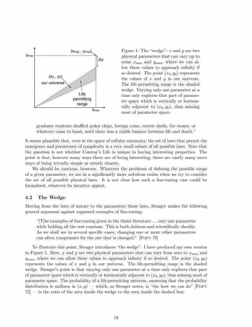
Figure 1: The “wedge”: x and y are twophysical parameters that can vary up tosome xmax and ymax, where we can al-low these values to approach infinity ifso desired. The point (x0, y0) representsthe values of x and y in our universe.The life-permitting range is the shadedwedge. Varying only one parameter at atime only explores that part of parame-ter space which is vertically or horizon-tally adjacent to (x0, y0), thus missingmost of parameter space.
graduate students shuffled poker chips, foreign coins, cowrie shells, Go stones, orwhatever came to hand, until there was a viable balance between life and death.”
It seems plausible that, even in the space of cellular automata, the set of laws that permit theemergence and persistence of complexity is a very small subset of all possible laws. Note thatthe question is not whether Conway’s Life is unique in having interesting properties. Thepoint is that, however many ways there are of being interesting, there are vastly many moreways of being trivially simple or utterly chaotic.
We should be cautious, however. Whatever the problems of defining the possible rangeof a given parameter, we are in a significantly more nebulous realm when we try to considerthe set of all possible physical laws. It is not clear how such a fine-tuning case could beformalised, whatever its intuitive appeal.
4.2 The Wedge
Moving from the laws of nature to the parameters those laws, Stenger makes the followinggeneral argument against supposed examples of fine-tuning:
“[T]he examples of fine-tuning given in the theist literature . . . vary one parameterwhile holding all the rest constant. This is both dubious and scientifically shoddy.As we shall see in several specific cases, changing one or more other parameterscan often compensate for the one that is changed.” [Foft 70]
To illustrate this point, Stenger introduces “the wedge”. I have produced my own versionin Figure 1. Here, x and y are two physical parameters that can vary from zero to xmax andymax, where we can allow these values to approach infinity if so desired. The point (x0, y0)represents the values of x and y in our universe. The life-permitting range is the shadedwedge. Stenger’s point is that varying only one parameter at a time only explores that partof parameter space which is vertically or horizontally adjacent to (x0, y0), thus missing most ofparameter space. The probability of a life-permitting universe, assuming that the probabilitydistribution is uniform in (x, y) — which, as Stenger notes, is “the best we can do” [Foft72] — is the ratio of the area inside the wedge to the area inside the dashed box.
19
4.2.1 The Wedge is a Straw Man
In response, fine-tuning relies on a number of independent life-permitting criteria. Fail anyof these criteria, and life becomes dramatically less likely, if not impossible. When parameterspace is explored in the scientific literature, it rarely (if ever) looks like the wedge. We insteadsee many intersecting wedges. Here are two examples.
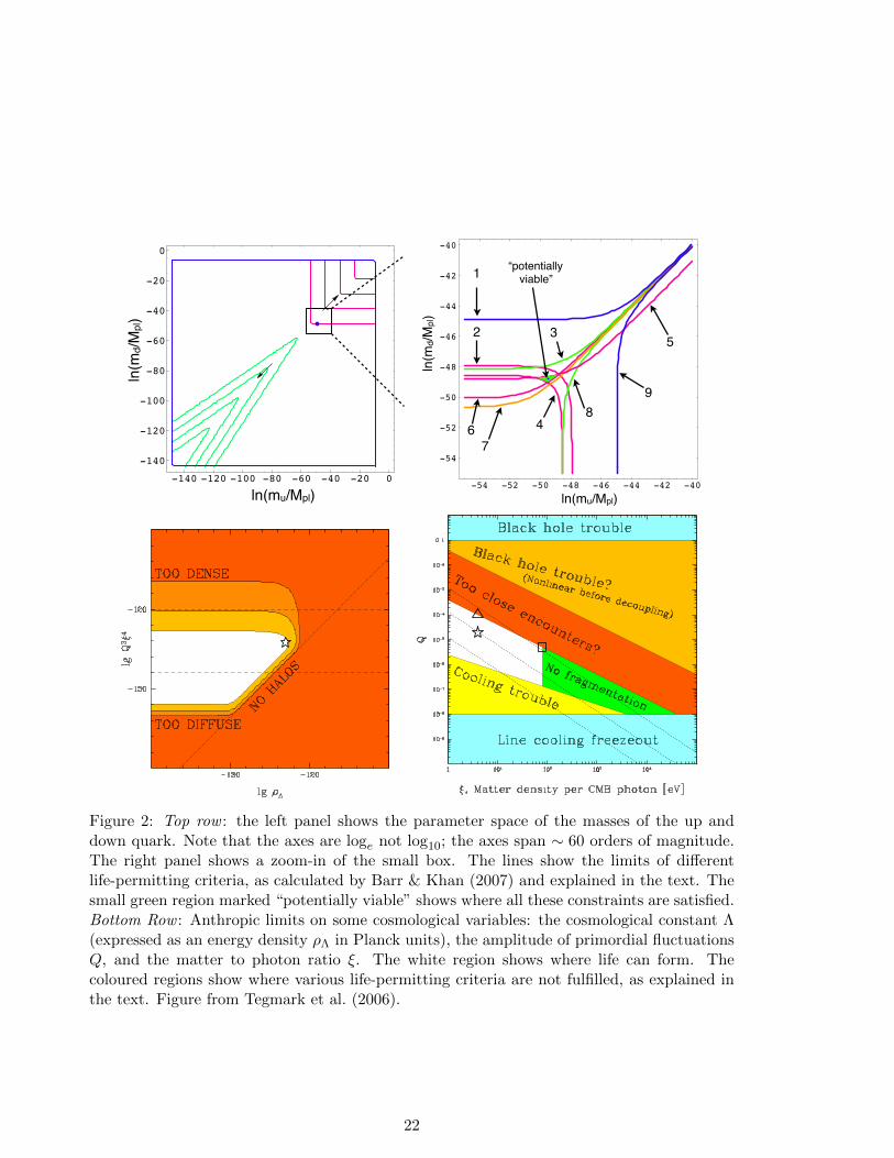
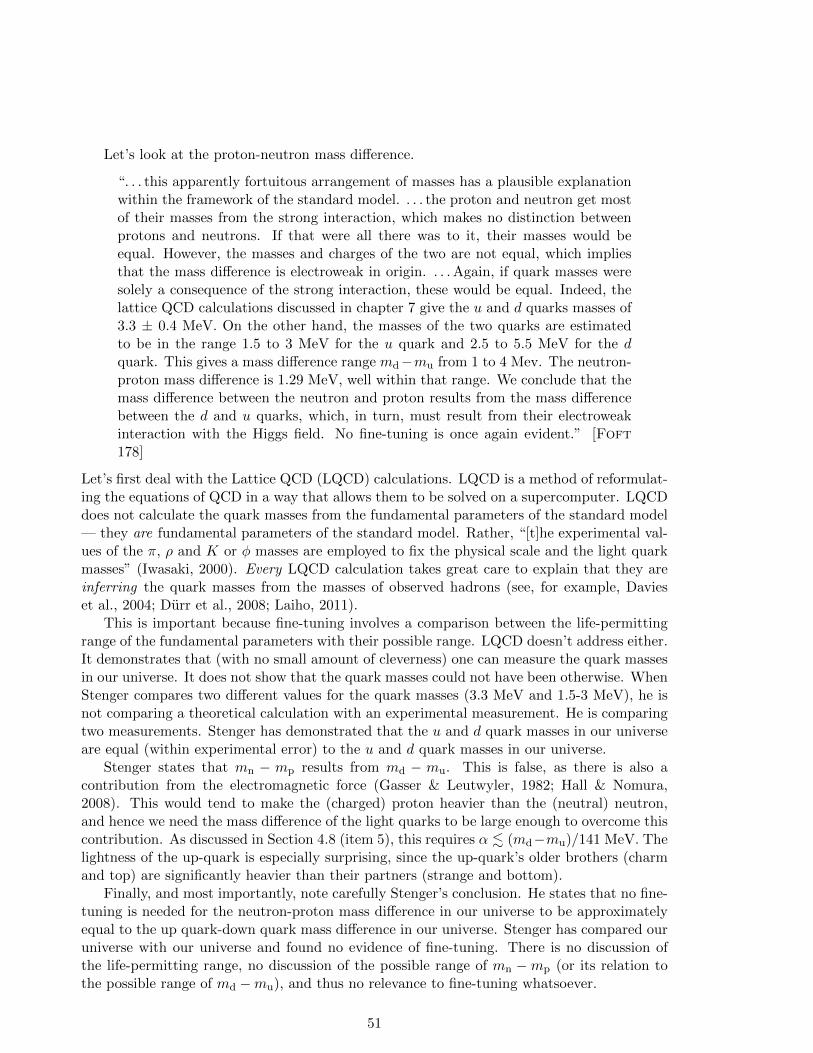
Barr & Khan (2007) explored the parameter space of a model in which up-type anddown-type fermions acquire mass from different Higgs doublets. As a first step, they vary themasses of the up and down quarks. The natural scale for these masses ranges over 60 ordersof magnitude and is illustrated in Figure 2 (top left). The upper limit is provided by thePlanck scale; the lower limit from dynamical breaking of chiral symmetry by QCD; see Barr& Khan (2007) for a justification of these values. Figure 2 (top right) zooms in on a regionof parameter space, showing boundaries of 9 independent life-permitting criteria:
1. Above the blue line, there is only one stable element, which consists of a single particle∆++. This element has the chemistry of helium — an inert, monatomic gas (above 4K) with no known stable chemical compounds.
2. Above this red line, the deuteron is strongly unstable, decaying via the strong force.The first step in stellar nucleosynthesis in hydrogen burning stars would fail.
3. Above the green curve, neutrons in nuclei decay, so that hydrogen is the only stableelement.
4. Below this red curve, the diproton is stable15. Two protons can fuse to helium-2 via avery fast electromagnetic reaction, rather than the much slower, weak nuclear pp-chain.
5. Above this red line, the production of deuterium in stars absorbs energy rather thanreleasing it. Also, the deuterium is unstable to weak decay.
6. Below this red line, a proton in a nucleus can capture an orbiting electron and becomea neutron. Thus, atoms are unstable.
7. Below the orange curve, isolated protons are unstable, leaving no hydrogen left overfrom the early universe to power long-lived stars and play a crucial role in organicchemistry.
8. Below this green curve, protons in nuclei decay, so that any atoms that formed woulddisintegrate into a cloud of neutrons.
9. Below this blue line, the only stable element consists of a single particle ∆−, whichcan combine with a positron to produce an element with the chemistry of hydrogen. A
15This may not be as clear-cut a disaster as is often asserted in the fine-tuning literature, going back toDyson (1971). MacDonald & Mullan (2009) and Bradford (2009) have shown that the binding of the diprotonis not sufficient to burn all the hydrogen to helium in big bang nucleosynthesis. For example, MacDonald &Mullan (2009) show that while an increase in the strength of the strong force by 13% will bind the diproton, a∼ 50% increase is needed to significantly affect the amount of hydrogen left over for stars. Also, Collins (2003)has noted that the decay of the diproton will happen too slowly for the resulting deuteron to be converted intohelium, leaving at least some deuterium to power stars and take the place of hydrogen in organic compounds.Finally with regard to stars, Phillips (1999, pg. 118) notes that: “It is sometimes suggested that the timescalefor hydrogen burning would be shorter if it were initiated by an electromagnetic reaction instead of the weaknuclear reaction [as would be the case is the diproton were bound]. This is not the case, because the overallrate for hydrogen burning is determined by the rate at which energy can escape from the star, i.e. by itsopacity, If hydrogen burning were initiated by an electromagnetic reaction, this reaction would proceed atabout the same rate as the weak reaction, but at a lower temperature and density.” However, stars in such auniverse would be significantly different to our own, and detailed predictions for their formation and evolutionhave not been investigated.
20
handful of chemical reactions are possible, with their most complex product being (ananalogue of) H2.
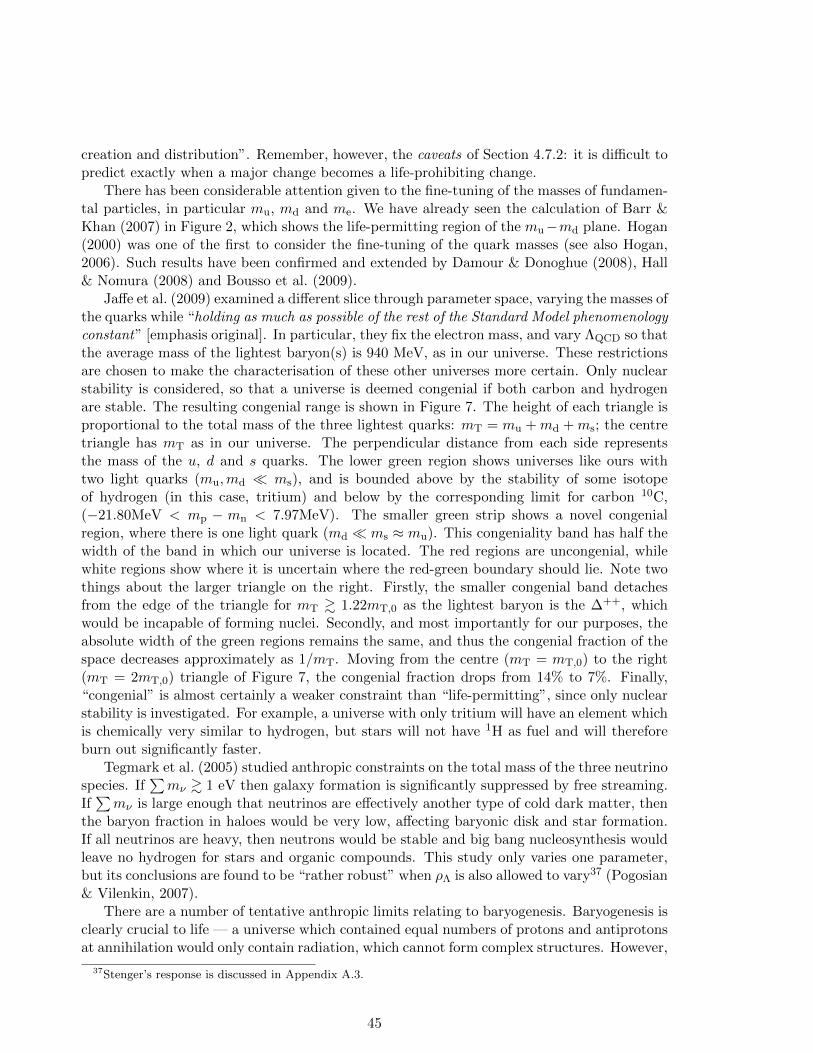
A second example comes from cosmology. Figure 2 (bottom row) comes from Tegmarket al. (2006). It shows the life-permitting range for two slices through cosmological parameterspace. The parameters shown are: the cosmological constant Λ (expressed as an energydensity ρΛ in Planck units), the amplitude of primordial fluctuations Q, and the matter tophoton ratio ξ. A star indicates the location of our universe, and the white region showswhere life can form. The left panel shows ρΛ vs. Q3ξ4. The red region shows universes thatare plausibly life-prohibiting — too far to the right and no cosmic structure forms; straytoo low and cosmic structures are not dense enough to form stars and planets; too high andcosmic structures are too dense to allow long-lived stable planetary systems. Note well thelogarithmic scale — the lack of a left boundary to the life-permitting region is because we havescaled the axis so that ρΛ = 0 is at x = −∞. The universe re-collapses before life can formfor ρΛ . −10−121 (Peacock, 2007). The right panel shows similar constraints in the Q vs. ξspace. We see similar constraints relating to the ability of galaxies to successfully form starsby fragmentation due to gas cooling and for the universe to form anything other than blackholes. Note that we are changing ξ while holding ξbaryon constant, so the left limit of the plotis provided by the condition ξ ≥ ξbaryon. See Table 4 of Tegmark et al. (2006) for a summaryof 8 anthropic constraints on the 7 dimensional parameter space (α, β,mp, ρΛ, Q, ξ, ξbaryon).
Examples could be multiplied, and the restriction to a 2D slice through parameter spaceis due to the inconvenient unavailability of higher dimensional paper. These two examplesshow that the wedge, by only considering a single life-permitting criterion, seriously distortstypical cases of fine-tuning by committing the sequential juggler fallacy (Section 2). Stengerfurther distorts the case for fine-tuning by saying:
“In the fine-tuning view, there is no wedge and the point has infinitesimal area,so the probability of finding life is zero.” [Foft 70]
No reference is given, and this statement is not true of the scientific literature. The wedge isa straw man.
4.2.2 The Straw Man is Winning
The wedge, distortion that it is, would still be able to support a fine-tuning claim. The proba-bility calculated by varying only one parameter is actually an overestimate of the probabilitycalculated using the full wedge. Suppose the full life-permitting criterion that defines thewedge is,
1− ε ≤ y/x
y0/x0≤ 1 + ε , (5)
where ε is a small number quantifying the allowed deviation from the value of y/x in ouruniverse. Now suppose that we hold x constant at its value in our universe. We conservativelyestimate the possible range of y by y0. Then, the probability of a life-permitting universeis Py = 2ε. Now, if we calculate the probability over the whole wedge, we find that Pw ≤ε/(1 + ε) ≈ ε, where we have an upper limit because we have ignored the area with y inside∆y, as marked in Figure 1. Thus16 Py ≥ Pw.
16Note that this is independent of xmax and ymax, and in particular holds in the limit xmax, ymax →∞.
21
-140 -120 -100 -80 -60 -40 -20 0xu ! ln!mu"MPl#
-140
-120
-100
-80
-60
-40
-20
0
xd!ln!m d"
MPl#
ln(mu/Mpl)
ln(m
d/Mpl)
-54 -52 -50 -48 -46 -44 -42 -40xu ! ln!mu"MPl#
-54
-52
-50
-48
-46
-44
-42
-40
xd!ln!m d"
MPl#
ln(mu/Mpl)
ln(m
d/Mpl)
“potentially viable”
2
1
4
3
76
8
5
9
Figure 2: Top row : the left panel shows the parameter space of the masses of the up anddown quark. Note that the axes are loge not log10; the axes span ∼ 60 orders of magnitude.The right panel shows a zoom-in of the small box. The lines show the limits of differentlife-permitting criteria, as calculated by Barr & Khan (2007) and explained in the text. Thesmall green region marked “potentially viable” shows where all these constraints are satisfied.Bottom Row : Anthropic limits on some cosmological variables: the cosmological constant Λ(expressed as an energy density ρΛ in Planck units), the amplitude of primordial fluctuationsQ, and the matter to photon ratio ξ. The white region shows where life can form. Thecoloured regions show where various life-permitting criteria are not fulfilled, as explained inthe text. Figure from Tegmark et al. (2006).
22
It is thus not necessarily “scientifically shoddy” to vary only one variable. Indeed, asscientists we must make these kind of assumptions all the time — the question is how accuratethey are. Under fairly reasonable assumptions (uniform probability etc.), varying only onevariable provides a useful estimate of the relevant probability. The wedge thus commits theflippant funambulist fallacy (Section 2). If ε is small enough, then the wedge is a tightrope.We have opened up more parameter space in which life can form, but we have also openedup more parameter space in which life cannot form. As Dawkins (1986) has rightly said:“however many ways there may be of being alive, it is certain that there are vastly more waysof being dead, or rather not alive”.
How could this conclusion be avoided? Perhaps the life-permitting region magically weavesits way around the regions left over from the vary-one-parameter investigation. The otheralternative is to hope for a non-uniform prior probability. One can show that a power-lawprior has no significant effect on the wedge. Any other prior raises a problem, as explainedby Aguirre in Carr (2007):
“. . . it is assumed that [the prior] is either flat or a simple power law, withoutany complicated structure. This can be done just for simplicity, but it is oftenargued to be natural. The flavour of this argument is as follows. If [the prior] is tohave an interesting structure over the relatively small range in which observers areabundant, there must be a parameter of order the observed [one] in the expressionfor [the prior]. But it is precisely the absence of this parameter that motivatedthe anthropic approach.”
In short, to significantly change the probability of a life-permitting universe, we would needa prior that centres close to the observed value, and has a narrow peak. But this simplyexchanges one fine-tuning for two — the centre and peak of the distribution.
There is, however, one important lesson to be drawn from the wedge. If we vary x only andcalculate Px, and then vary y only and calculate Py, we must not simply multiply Pw = Px Py.This will certainly underestimate the probability inside the wedge, assuming that there is onlya single wedge.
4.3 Entropy
We turn now to cosmology. The problem of the apparently low entropy of the universe is oneof the oldest problems of cosmology. The fact that the entropy of the universe is not at itstheoretical maximum, coupled with the fact that entropy cannot decrease, means that theuniverse must have started in a very special, low entropy state. Stenger replies as follows.Bekenstein (1973) and Hawking (1975) showed that a black hole has an entropy equal to aquarter of its horizon area,
SBH =A
4= πR2
S , (6)
where RS is the radius of the black hole event horizon, the Schwarzschild radius. Now, insteadof a black hole, suppose we consider an expanding universe of radius RH = c/H, where H isthe Hubble parameter. The “Schwarzschild radius” of the observable universe is
RS = 2M =8π
3ρR3
H = RH , (7)
where we have used the Friedmann equation, H2 = 8πρ/3, and ρ “is the sum of all the con-tributions to the mass/energy of the universe: matter, radiation, curvature, and cosmological
23
constant” [Foft 111]. Thus, the observable universe has entropy equal to a black hole of thesame radius. In particular, if the universe starts out at the Planck time as a sphere of radiusequal to the Planck length, then its entropy is as great as it could possibly be, equal to thatof a Planck-sized black hole.
Now, consider a region of radius R (and volume V ) inside the expanding universe. Themaximum entropy is given by SBH(R) (Equation 6), while the actual entropy is the region’sshare (by volume) of the total entropy of the observable universe. The difference betweenmaximum and actual entropy is
Smax − Sactual = πR2 − πR2H
V
VH= πR2
(1− R
RH
). (8)
Thus, the expansion of the universe opens up regions of size R, smaller than the observableuniverse. In such regions, the expansion of the universe opens up an entropy gap. “As long asR < RH , order can form without violating the second law of thermodynamics” [Foft 113].
Note that Stenger’s proposed solution requires only two ingredients — the initial, high-entropy state, and the expansion of the universe to create an entropy gap. In particular,Stenger is not appealing to inflation to solve the entropy problem. We will do the same inthis section, coming to a discussion of inflation later.
There are good reasons to be sceptical. This solution to one of the deepest problemsin physics — the origin of the second law of thermodynamics and the arrow of time — issuspiciously missing from the scientific literature. Stenger is not reporting the consensusof the scientific community; neither is he using rough approximations to summarise a morecareful, more technical calculation that has passed peer review.
Applying the Bekenstein limit to a cosmological spacetime is not nearly as straightforwardas Stenger implies. The Bekenstein limit applies to the event horizon of a black hole. TheHubble radius RH is not any kind of horizon. It is the distance at which the proper recessionvelocity of the Hubble flow is equal to the speed of light. There is no causal limit associatedwith the Hubble radius as information and particles can pass both ways, and can reach theobserver at the origin (Davis & Lineweaver, 2004). Further, given that the entropy in questionis associated with the surface area of an event horizon, it not obvious that one can distributesaid entropy uniformly over the enclosed volume, as in Equation 8.
Even in terms of the Hubble radius, Stenger’s calculation is mistaken. Stenger says thatρ is “the sum of all the contributions to the mass/energy of the universe: matter, radiation,curvature, and cosmological constant”. This is incorrect. Specifically, there is no such thingas curvature energy. The term involving the curvature in the Friedmann equation does notrepresent a form of energy; it comes from the geometry side of the Einstein equation, notthe energy-momentum side. Curvature energy is “just a notational sleight of hand” (Carroll,2003, pg. 338). Remember that the curvature in question is space curvature, not spacetimecurvature, and thus has no coordinate independent meaning. More generally, there is no suchthing as gravitational energy in general relativity (Misner et al., 1973, pg. 467). Equation7 only holds if the universe is exactly flat, and thus Stenger has at best traded the entropyproblem for the flatness problem.
What if we consider the cosmic event horizon instead of the Hubble radius? The (comovingdistance to the) event horizon in an FLRW spacetime is given by dE =
∫∞0 c dt/a(t), where
a(t) is the scale factor of the universe. This integral may not converge, in which case thereis no event horizon. In the concordance model of cosmology, it does converge thanks to thecosmological constant. Its value is around dE ≈ 20 Gpc comoving, which corresponds to a
24
physical scale of around 3× 10⁻⁵m at the Planck time. It is then not true that at the Plancktime the “Schwarzschild radius” of the universe (around 3 × 10⁻³⁵ metres) is equal to thedistance to its event horizon.
Perhaps we should follow the advice of Bekenstein (1989) and consider the particle horizonat the Planck time, defined by dp(tPl) =
∫ tPl
0 c dt/a(t). This is, in general, not equal to theHubble radius, though if the universe is radiation dominated in its earliest stages then the twoare actually equal. The problem now is somewhat deeper. The reason that we are consideringthe Planck time is that we would need a quantum theory of spacetime to be able to predictwhat happened before this time. In fact, our best guess is that classical notions of spacetimeare meaningless before tPl, to be replaced with a quantum spacetime “foam”. However, thedefinition of dp requires us to integrate a(t) from t = 0 to tPl. The very reason that weare considering the universe at tPl is therefore sufficient reason to reject the validity of ourcalculation of the particle horizon.
There is no consensus on how to correctly apply the Bekenstein limit to cosmology. Beken-stein (1989), as noted above, argued that one should apply the black hole entropy bound tothe particle horizon of the universe. Gibbons & Hawking (1977) and Davies (1988) consideredthe thermodynamic properties of cosmic event horizons; Davis et al. (2003) noted that notall FLRW spacetimes respect the generalised second law of thermodynamics. There are otherways of formulating the entropy bound on a cosmological region. For example, Brustein &Veneziano (2000) formulate the causal entropy bound on space-like hypersurfaces. The re-view of Bousso (2002) notes that “a naive generalisation of the spherical entropy bound isunsuccessful. . . . [T]he idea that the area of surfaces generally bounds the entropy in enclosedspatial volumes has proven wrong. . . . [A] general entropy bound, if found, is no triviality”.Bousso defends the covariant entropy bound, defined using light sheets in general relativity.
Further problems arise even if we assume that Stenger’s argument is correct. Stengerhas asked us to consider the universe at the Planck time, and in particular a region of theuniverse that is the size of the Planck length. Let’s see what happens to this comoving volumeas the universe expands. 13.7 billion years of (concordance model) expansion will blow upthis Planck volume until it is roughly the size of a grain of sand. A single Planck volume ina maximum entropy state at the Planck time is a good start but hardly sufficient. To makeour universe, we would need around 1090 such Planck volumes, all arranged to transition toa classical expanding phase within a temporal window 100,000 times shorter than the Plancktime17. This brings us to the most serious problem with Stenger’s reply.
Let’s remind ourselves of what the entropy problem is, as expounded by Penrose (1979).Consider our universe at t1 = one second after the big bang. Spacetime is remarkably smooth,represented by the Robertson-Walker metric to better than one part in 105. Now run the clockforward. The tiny inhomogeneities grow under gravity, forming deeper and deeper potentialwells. Some will collapse into black holes, creating singularities in our once pristine spacetime.Now suppose that the universe begins to recollapse. Unless the collapse of the universe wereto reverse the arrow of time18, entropy would continue to increase, creating more and larger
17This requirement is set by the homogeneity of our universe. Regions that transition early will expand anddilute, and so for the entire universe to be homogeneous to within Q ≈ 10−5, the regions must begin theirclassical phase within ∆t ≈ Qt.
18This seems very unlikely. Regions of the universe which have collapsed and virialised have decoupled fromthe overall expansion of the universe, and so would have no way of knowing exactly when the expansion stalledand reversed. However, as Price (1997) lucidly explains, such arguments risk invoking a double standard, asthey work just as well when applied backwards in time.
25
inhomogeneities and black holes as structures collapse and collide. If we freeze the universeat t2 = one second before the big crunch, we see a spacetime that is highly inhomogeneous,littered with lumps and bumps, and pockmarked with singularities.
Penrose’s reasoning is very simple. If we started at t1 with an extremely homogeneousspacetime, and then allowed a few billion years of entropy increasing processes to take theirtoll, and ended at t2 with an extremely inhomogeneous spacetime, full of black holes, thenwe must conclude that the t2 spacetime represents a significantly higher entropy state thanthe t1 spacetime19. We conclude that we know what a high entropy big bang spacetime lookslike, and it looks nothing like the state of our universe in its earliest stages. Why didn’t ouruniverse begin in a high entropy, highly inhomogeneous state? Why did our universe startoff in such a special, improbable, low-entropy state?
Let’s return to Stenger’s proposed solution. After introducing the relevant concepts, hesays [Foft 112]:
“. . . this does not mean that the local entropy is maximal. The entropy density ofthe universe can be calculated. Since the universe is homogeneous, it will be thesame on all scales.”
Stenger takes it for granted that the universe is homogeneous and isotropic. We can see thisalso in his use of the Friedmann equation, which assumes that spacetime is homogeneous andisotropic. Not surprisingly, once homogeneity and isotropy have been assumed, Stenger findsthat the solution to the entropy problem is remarkably easy.
We conclude that Stenger has not only failed to solve the entropy problem; he has failedto comprehend it. He has presented the problem itself as its solution. Homogeneous, isotropicexpansion cannot solve the entropy problem — it is the entropy problem. Stenger’s asser-tion that “the universe starts out with maximum entropy or complete disorder” is false. Ahomogeneous, isotropic spacetime is an incredibly low entropy state. Penrose (1989) warnedof precisely this brand of failed solution two decades ago:
“Virtually all detailed investigations [of entropy and cosmology] so far have takenthe FRW models as their starting point, which, as we have seen, totally begs thequestion of the enormous number of degrees of freedom available in the gravi-tational field . . . The second law of thermodynamics arises because there was anenormous constraint (of a very particular kind) placed on the universe at the be-ginning of time, giving us the very low entropy that we need in order to startthings off.”
Cosmologists repented of such mistakes in the 1970’s and 80’s.Stenger’s “biverse” [Foft 142] doesn’t solve the entropy problem either. Once again,
homogeneity and isotropy are simply assumed, with the added twist that instead of a lowentropy initial state, we have a low entropy middle state. This makes no difference — thereason that a low entropy state requires explanation is that it is improbable. Moving theimprobable state into the middle does not make it any more probable. As Carroll (2008) notes,“an unnatural low-entropy condition [that occurs] in the middle of the universe’s history (atthe bounce) . . . passes the buck on the question of why the entropy near what we call the bigbang was small”.20
19Recall that, if the two spacetimes can still be described on large scales by the Robertson-Walker metric,then their large scale properties will be identical, except for the sign of the Hubble parameter.
20Foft 142 tells us that Carroll has actually raised this objection to Stenger, whose reply was to point out
26
4.4 Inflation
4.4.1 Did Inflation Happen?
We turn now to cosmic inflation, which proposes that the universe underwent a period ofaccelerated expansion in its earliest stages. The achievements of inflation are truly impressive— in one fell swoop, the universe is sent on its expanding way, the flatness, horizon, andmonopole problem are solved and we have concrete, testable and seemingly correct predictionsfor the origin of cosmic structure. It is a brilliant idea, and one that continues to defy allattempts at falsification. Since life requires an almost-flat universe (Barrow & Tipler, 1986,pg. 408ff.), inflation is potentially a solution to a particularly impressive fine-tuning problem— sans inflation, the density of the universe at the Planck time must be tuned to 60 decimalplaces in order for the universe to be life-permitting.
Inflation solves this fine-tuning problem by invoking a dynamical mechanism that drivesthe universe towards flatness. The first question we must ask is: did inflation actually happen?The evidence is quite strong, though not indubitable (Turok, 2002; Brandenberger, 2011).There are a few things to keep in mind. Firstly, inflation isn’t a specific model as such; it isa family of models which share the desirable trait of having an early epoch of acceleratingexpansion. Inflation is an effect, rather than a cause. There is no physical theory that predictsthe form of the inflaton potential. Different potentials, and different initial conditions for thesame potential, will produce different predictions.
In spite of this, inflation does provide some robust predictions, that is, predictions sharedby a wide variety of inflationary potentials. The problem is that these predictions are notunique to inflation. Inflation predicts a Gaussian random field of density fluctuations, butthanks to the central limit theorem this is nothing particularly unique (Peacock, 1999, pg.342, 503). Inflation predicts a nearly scale-invariant spectrum of fluctuations, but such aspectrum was proposed for independent reasons by Harrison (1970) and Zel’dovich (1972) adecade before inflation was proposed. Inflation is a clever solution of the flatness and horizonproblem, but could be rendered unnecessary by a quantum-gravity theory of initial conditions.The evidence for inflation is impressive but circumstantial.
4.4.2 Can Inflation Explain Fine-tuning?
Note the difference between this section and the last. Is inflation itself fine-tuned? This is nomere technicality — if the solution is just as fine-tuned as the problem, then no progress hasbeen made. Inflation, to set up a life-permitting universe, must do the following21:
I1. There must be an inflaton field. To make the expansion of the universe accelerate, theremust exist a form of energy (a field) capable of satisfying the so-called Slow Roll Approx-imation (SRA), which is equivalent to requiring that the potential energy of the field ismuch greater than its kinetic energy, giving the field negative pressure.
that the arrow of time always points away from the lowest entropy point, so we can always call that point thebeginning of the universe. Once again, Stenger fails to understand the problem. The question is not why thelow entropy state was at the beginning of the universe, but why the universe was ever in a low entropy state.The second law of thermodynamics tells us that the most probable world is one in which the entropy is alwayshigh, and thus has no significant entropy gradients. This is precisely what entropy quantifies. See Price (1997,2006) for an excellent discussion of these issues.
21These requirements can be found in any good cosmology textbook, e.g. Peacock (1999); Mo et al. (2010).
27
I2. Inflation must start. There must come a time in the history of the universe when theenergy density of the inflaton field dominates the total energy density of the universe,dictating its dynamics.
I3. Inflation must last. While the inflaton field controls the dynamics of the expansion of theuniverse, we need it to obey the slow roll conditions for a sufficiently long period of time.The “amount of inflation” is usually quantified by Ne, the number of e-folds of the sizeof the universe. To solve the horizon and flatness problems, this number must be greaterthan ∼ 60.
I4. Inflation must end. The dynamics of the expansion of the universe will (if it expandsforever) eventually be dominated by the energy component with the most negative equa-tion of state w = pressure / energy density. Matter has w = 0, radiation w = 1/3, andtypically during inflation, the inflaton field has w ≈ −1. Thus, once inflation takes over,there must be some special reason for it to stop; otherwise, the universe would maintainits exponential expansion and no complex structure would form.
I5. Inflation must end in the right way. Inflation will have exponentially diluted the mass-energy density of the universe — it is this feature that allows inflation to solve themonopole problem. Once we are done inflating the universe, we must reheat the universe,i.e. refill it with ordinary matter. We must also ensure that the post-inflation fielddoesn’t possess a large, negative potential energy, which would cause the universe toquickly recollapse.
I6. Inflation must set up the right density perturbations. Inflation must result in a universethat is very homogeneous, but not perfectly homogeneous. Inhomogeneities will growvia gravitational instability to form cosmic structures. The level of inhomogeneity (Q) issubject to anthropic constraints, which we will discuss in Section 4.5.
The question now is: which of these achievements come naturally to inflation, and whichneed some careful tuning of the inflationary dials? I1 is a bare hypothesis — we know of nodeeper reason why there should be an inflaton field at all. It was hoped that the inflaton fieldcould be the Higgs field (Guth, 1981). Alas, it wasn’t to be, and it appears that the inflaton’ssole raison d’etre is to cause the universe’s expansion to briefly accelerate. There is no directevidence for the existence of the inflaton field.
We can understand many of the remaining conditions through the work of Tegmark (2005),who considered a wide range of inflaton potentials using Gaussian random fields. The po-tential is of the form V (φ) = m4
vf( φmh
), where mv and mh are the characteristic vertical andhorizontal mass scales, and f is a dimensionless function with values and derivatives of orderunity. For initial conditions, Tegmark “sprays starting points randomly across the potentialsurface”. Figure 3 shows a typical inflaton potential.
Requirement I2 will be discussed in more detail below. For now we note that the inflatonmust either begin or be driven into a region in which the SRA holds in order for the universeto inflate, as shown by the thick lines in Figure 3.
Requirement I3 comes rather naturally to inflation: Peacock (1999, pg. 337) shows thatthe requirement that inflation produce a large number of e-folds is essentially the same as therequirement that inflation happen in the first place (i.e. SRA), namely φstart mPl. Thisassumes that the potential is relatively smooth, and that inflation terminates at a value ofthe field (φ) rather smaller than its value at the start. There is another problem lurking,however. If inflation lasts for & 70 e-folds (for GUT scale inflation), then all scales inside
28
0 20 40 60
-0.01
0
0.01
Figure 3: An example of a randomly-generated inflaton potential. Thicklines show where the Slow Roll Ap-proximation holds (SRA); thin linesshow where it fails. The stars showfour characteristic initial conditions.Three-pointed: the inflaton starts out-side the SRA regions and does not re-enter, so there is no inflation. Four-pointed: successful inflation. Inflationwill have a beginning, and end, and thepost-inflationary vacuum energy is suf-ficiently small to allow the growth ofstructure. Five-pointed: inflation oc-curs, but the post-inflation field has alarge, negative potential energy, whichwould cause the universe to quickly rec-ollapse. Six-pointed: inflation neverends, and the universe contains no or-dinary matter and no structure. Figurefrom Tegmark (2005).
the Hubble radius today started out with physical wavelength smaller than the Planck scaleat the beginning of inflation (Brandenberger, 2011). The predictions of inflation (especiallythe spectrum of perturbations), which use general relativity and a semi-classical descriptionof matter, must omit relevant quantum gravitational physics. This is a major unknown —transplanckian effects may even prevent the onset of inflation.
I4 is non-trivial. The inflaton potential (or, more specifically, the region of the inflatonpotential which actually determines the evolution of the field) must have a region in whichthe slow-roll approximation does not hold. If the inflaton rolls into a local minimum (at φ0)while the SRA still holds (which requires V (φ0) m2
Pl/8π d2V/dφ2|φ0 Peacock, 1999, pg.332), then inflation never ends.
Tegmark (2005) asks what fraction of initial conditions for the inflaton field are success-ful, where success means that the universe inflates, inflation ends and the universes doesn’tthereafter meet a swift demise via a big crunch. The result is shown in Figure 4. The thickblack line shows the “success rate” of inflation, for a model with mh/mPl as shown on thex-axis and mv = 0.001mPl. (This value has been chosen to maximise the probability thatQ = Qobserved ≈ 2 × 10⁻⁵). The coloured curves show predictions for other cosmologicalparameters. The lower coloured regions are for mv = 0.001mPl; the upper coloured regionsare for mv = mh. The success rate peaks at ∼ 0.1 percent, and drops rapidly as mh increasesor decreases away from mPl. Even with a scalar field, inflation is far from guaranteed.
If inflation ends, we need its energy to be converted into ordinary matter (Condition I5).Inflation must not result in a universe filled with pure radiation or dark matter, which cannotform complex structures. Typically, the inflaton will to dump its energy into radiation. Thetemperature must be high enough to take advantage of baryon-number-violating physics forbaryogenesis, and for γ+γ → particle + antiparticle reactions to create baryonic matter, but
29
Figure 4: The thick black line showsthe “success rate” of inflation, for amodel with mh/mPl as shown on thex-axis and mv = 0.001mPl. (This valuehas been chosen to maximise the prob-ability of Q = Qobserved ≈ 2 × 10⁻⁵).The success rate is at most ∼ 0.1%.The other coloured curves show pre-dictions for other cosmological parame-ters. The lower coloured regions are formv = 0.001mPl; the upper coloured re-gions are for mv = mh. Figure adaptedfrom Tegmark (2005).
low enough not to create magnetic monopoles. With no physical model of the inflaton, thenecessary coupling between the inflaton and ordinary matter/radiation is another postulate,but not an implausible one.
Requirement I6 brought about the downfall of “old” inflation. When this version ofinflation ended, it did so in expanding bubbles. Each bubble is too small to account for thehomogeneity of the observed universe, and reheating only occurs when bubbles collide. Asthe space between the bubbles is still inflating, homogeneity cannot be achieved. New modelsof inflation have been developed which avoid this problem. More generally, the value of Qthat results from inflation depends on the potential and initial conditions. We will discuss Qfurther in Section 4.5.
Perhaps the most pressing issue with inflation is hidden in requirement I2. Inflation issupposed to provide a dynamical explanation for the seemingly very fine-tuned initial condi-tions of the standard model of cosmology. But does inflation need special initial conditions?Can inflation act on generic initial conditions and produce the apparently fine-tuned uni-verse we observe today? Hollands & Wald (2002b)22 contend not, for the following reason.Consider a collapsing universe. It would require an astonishing sequence of correlations andcoincidences for the universe, in its final stages, to suddenly and coherently convert all itsmatter into a scalar field with just enough kinetic energy to roll to the top of its potentialand remain perfectly balanced there for long enough to cause a substantial era of “deflation”.The region of final-condition-space that results from deflation is thus much smaller than theregion that does not result from deflation. Since the relevant physics is time-reversible23, wecan simply run the tape backwards and conclude that the initial-condition-space is dominatedby universes that fail to inflate.
Readers will note the similarity of this argument to Penrose’s argument from Section4.3. This intuitive argument can be formalised using the work of Gibbons et al. (1987), whodeveloped the canonical measure on the set of solutions of Einstein’s equation of GeneralRelativity. A number of authors have used the Gibbons-Hawking-Stewart canonical measureto calculate the probability of inflation; see Hawking & Page (1988), Gibbons & Turok (2008)
22See also the discussion in Kofman et al. (2002) and Hollands & Wald (2002a)23Cosmic phase transitions are irreversible in the same sense that scrambling an egg is irreversible. The time
asymmetry is a consequence of low entropy initial conditions, not the physics itself (Penrose, 1989; Hollands& Wald, 2002a).
30
and references therein. We will summarise the work of Carroll & Tam (2010), who ask whatfraction of universes that evolve like our universe since matter-radiation equality could havebegun with inflation. Crucially, they consider the role played by perturbations:
“Perturbations must be sub-dominant if inflation is to begin in the first place(Vachaspati & Trodden, 1999), and by the end of inflation only small quantumfluctuations in the energy density remain. It is therefore a necessary (althoughnot sufficient) condition for inflation to occur that perturbations be small at earlytimes. . . . the fraction of realistic cosmologies that are eligible for inflation istherefore P (inflation) ≈ 10−6.6×10⁷ .”
Carroll & Tam casually note: “This is a small number”, and in fact an overestimate. Anegligibly small fraction of universes that resemble ours at late times experience an earlyperiod of inflation. Carroll & Tam (2010) conclude that while inflation is not without itsattractions (e.g. it may give a theory of initial conditions a slightly easier target to hit at thePlanck scale), “inflation by itself cannot solve the horizon problem, in the sense of making thesmooth early universe a natural outcome of a wide variety of initial conditions”. Note thatthis argument also shows that inflation, in and of itself, cannot solve the entropy problem24.
Let’s summarise. Inflation is a wonderful idea; in many ways it seems irresistible (Liddle,1995). However, we do not have a physical model, and even we had such a model, “althoughinflationary models may alleviate the “fine tuning” in the choice of initial conditions, themodels themselves create new “fine tuning” issues with regard to the properties of the scalarfield” (Hollands & Wald, 2002b). To pretend that the mere mention of inflation makes alife-permitting universe “100 percent” inevitable [Foft 245] is naıve in the extreme, a canetoad solution. For a popular-level discussion of many of the points raised in our discussion ofinflation, see Steinhardt (2011).
4.4.3 Inflation as a Case Study
Suppose that inflation did solve the fine-tuning of the density of the universe. Is it reasonableto hope that all fine-tuning cases could be solved in a similar way? We contend not, becauseinflation has a target. Let’s consider the range of densities that the universe could have hadat some point in its early history. One of these densities is physically singled out as special —the critical density25. Now let’s note the range of densities that permit the existence of cosmicstructure in a long-lived universe. We find that this range is very narrow. Very conveniently,this range neatly straddles the critical density.
We can now see why inflation has a chance. There is in fact a three-fold coincidence — A:the density needed for life, B: the critical density, and C: the actual density of our universe areall aligned. B and C are physical parameters, and so it is possible that some physical processcan bring the two into agreement. The coincidence between A and B then creates the requiredanthropic coincidence (A and C). If, for example, life required a universe with a density (say,just after reheating) 10 times less than critical, then inflation would do a wonderful job ofmaking all universes uninhabitable.
24We should also note that Carroll & Tam (2010) argue that the Gibbons-Hawking-Stewart canonical measurerenders an inflationary solution to the flatness problem superfluous. This is a puzzling result — it would seemto show that non-flat FLRW universes are infinitely unlikely, so to speak. This result has been noted before.See Gibbons & Turok (2008) for a different point of view.
25We use the Hubble constant to specify the particular time being considered.
31
Inflation thus represents a very special case. Waiting inside the life-permitting range (L)is another physical parameter (p). Aim for p and you will get L thrown in for free. This is nottrue of the vast majority of fine-tuning cases. There is no known physical scale waiting in thelife-permitting range of the quark masses, fundamental force strengths or the dimensionalityof spacetime. There can be no inflation-like dynamical solution to these fine-tuning problemsbecause dynamical processes are blind to the requirements of intelligent life.
What if, unbeknownst to us, there was such a fundamental parameter? It would needto fall into the life-permitting range. As such, we would be solving a fine-tuning problemby creating at least one more. And we would also need to posit a physical process able todynamically drive the value of the quantity in our universe toward p.
4.5 The Amplitude of Primordial Fluctuations Q
Q, the amplitude of primordial fluctuations, is one of Martin Rees’ Just Six Numbers. In ouruniverse, its value is Q ≈ 2 × 10⁻⁵, meaning that in the early universe the density at anypoint was typically within 1 part in 100,000 of the mean density. What if Q were different?
“If Q were smaller than 10−6, gas would never condense into gravitationally boundstructures at all, and such a universe would remain forever dark and featureless,even if its initial ‘mix’ of atoms, dark energy and radiation were the same as ourown. On the other hand, a universe where Q were substantially larger than 10−5
— were the initial “ripples” were replaced by large-amplitude waves — would bea turbulent and violent place. Regions far bigger than galaxies would condenseearly in its history. They wouldn’t fragment into stars but would instead collapseinto vast black holes, each much heavier than an entire cluster of galaxies in ouruniverse . . . Stars would be packed too close together and buffeted too frequentlyto retain stable planetary systems.” (Rees, 1999, pg. 115)
Stenger has two replies. Firstly:
“[T]he inflationary model predicted that the deviation from smoothness shouldbe one part in 100,000. This prediction was spectacularly verified by the CosmicBackground Explorer (COBE) in 1992 [Foft 106] . . . While heroic attempts bythe best minds in cosmology have not yet succeeded in calculating the magnitudeof Q, inflation theory successfully predicted the angular correlation across the skythat has been observed.” [Foft 206]
Note that the first part of the quote contradicts the second part. We are first told thatinflation predicts Q = 10−5, and then we are told that inflation cannot predict Q at all.Both claims are false. A given inflationary model will predict Q, and it will only predict alife-permitting value for Q if the parameters of the inflaton potential are suitably fine-tuned.As Turok (2002) notes, “to obtain density perturbations of the level required by observations. . . we need to adjust the coupling µ [for a power law potential µφn] to be very small, ∼ 10−13
in Planck units. This is the famous fine-tuning problem of inflation”; see also Barrow &Tipler (1986, pg. 437) and Brandenberger (2011). Rees’ life-permitting range for Q impliesa fine-tuning of the inflaton potential of ∼ 10−11 with respect to the Planck scale. Tegmark(2005, particularly Figure 11) argues that on very general grounds we can conclude that life-permitting inflation potentials are highly unnatural. Susskind (2005, pg. 184) summarisesthe situation as follows:
32
“A lumpiness [Q] of about 10−5 is essential for life to get a start. But is it easy toarrange this amount of density contrast? The answer is most decidedly no! Thevarious parameters governing the inflating universe must be chosen with greatcare in order to get the desired result.”
Stenger’s second reply is to ask
“. . . is an order of magnitude fine-tuning? Furthermore, Rees, as he admits, isassuming all other parameters are unchanged. In the first case where Q is toosmall to cause gravitational clumping, increasing the strength of gravity would in-crease the clumping. Now, as we have seen, the dimensionless strength of gravityαG is arbitrarily defined. However, gravity is stronger when the masses involvedare greater. So the parameter that would vary along with Q would be the nu-cleon mass. As for larger Q, it seems unlikely that inflation would ever result inlarge fluctuations, given the extensive smoothing that goes on during exponentialexpansion.” [Foft 207]
There are a few problems here. We have a clear case of the flippant funambulist fallacy —the possibility of altering other constants to compensate the change in Q is not evidenceagainst fine-tuning. Choose Q and, say, αG at random and you are unlikely to have pickeda life-permitting pair, even if our universe is not the only life-permitting one. We also havea nice example of the cheap-binoculars fallacy. The allowed change in Q relative to its valuein our universe (“an order of magnitude”) is necessarily an underestimate of the degree offine-tuning. The question is whether this range is small compared to the possible range ofQ. Stenger seems to see this problem, and so argues that large values of Q are unlikelyto result from inflation. This claim is false, and symptomatic of Stenger’s tenuous grasp ofcosmology26. The upper blue region of Figure 4 shows the distribution of Q for the model ofTegmark (2005), using the “physically natural expectation” mv = mh. The mean value of Qranges from 10 to almost 10000.
Note that Rees only varies Q in “Just Six Numbers” because it is a popular level book.He and many others have extensively investigated the effect on structure formation of alteringa number of cosmological parameters, including Q.
• Tegmark & Rees (1998) were the first to calculate the range of Q which permits life,deriving the following limits for the case where ρΛ = 0:
α−1 ln(α−2)−16/9 αG (β/ξ)4/3Ω−2/3b . Q . α16/7α
4/7G β12/7ξ−8/7 , (9)
where these quantities are defined in Table 1, except for the cosmic baryon densityparameter Ωb, and we have omitted geometric factors of order unity. This inequalitydemonstrates the variety of physical phenomena, atomic, gravitational and cosmological,that must combine in the right way in order to produce a life-permitting universe.Tegmark & Rees also note that there is some freedom to change Q and ρΛ together.
• Tegmark et al. (2006) expanded on this work, looking more closely at the role of thecosmological constant. We have already seen some of the results from this paper in Sec-tion 4.2.1. The paper considers 8 anthropic constraints on the 7 dimensional parameterspace (α, β,mp, ρΛ, Q, ξ, ξbaryon). Figure 2 (bottom row) shows that the life-permitting
26More examples are compiled in Appendix A.
33
region is boxed-in on all sides. In particular, the freedom to increase Q and ρΛ togetheris limited by the life-permitting range of galaxy densities.
• Bousso et al. (2009) considers the 4-dimensional parameter space (β,Q, Teq, ρΛ), whereTeq is the temperature if the CMB at matter-radiation equality. The calculate theposition of what they call “catastrophic boundaries” in this space, across which theprobability of a universe being life-permitting drops dramatically. These boundariesarise from the ability of galaxies to cool and form stars, and the disruption of haloformation by the cosmological constant. They are primarily interested in using anthropiclimits to make predictions from the multiverse. Bousso & Leichenauer (2009) andBousso & Leichenauer (2010) refine these arguments using a “semianalytic” model forstar-formation as a function of cosmic time. They take particular care to consider theeffects of altering the various parameters simultaneously. While there is some freedom toincrease both Q and ρΛ while holding Q3/ρΛ constant, for Q & 10−3 vacuum dominationoccurs before recombination and stars will not form. (See also the earlier paper byGarriga et al., 1999).
• Garriga & Vilenkin (2006) discuss what they call the “Q catastrophe”: the probabilitydistribution for Q across a multiverse typically increases or decreases sharply throughthe anthropic window. Thus, we expect that the observed value of Q is very likely to beclose to one of the boundaries of the life-permitting range. The fact that we appear to bein the middle of the range leads Garriga & Vilenkin to speculate that the life-permittingrange may be narrower than Tegmark & Rees (1998) calculated. For example, theremay be a tighter upper bound due to the perturbation of comets by nearby stars and/orthe problem of nearby supernovae explosions.
• The interested reader is referred to the 90 scientific papers which cite Tegmark & Rees(1998), catalogued on the NASA Astrophysics Data System27.
The fine-tuning of Q stands up well under examination.
4.6 Cosmological Constant Λ
The cosmological constant problem is described in the textbook of Burgess & Moore (2006)as “arguably the most severe theoretical problem in high-energy physics today, as measuredby both the difference between observations and theoretical predictions, and by the lack ofconvincing theoretical ideas which address it”. A well-understood and well-tested theory offundamental physics (Quantum Field Theory — QFT) predicts contributions to the vacuumenergy of the universe that are ∼ 10120 times greater than the observed total value. Stenger’sreply is guided by the following principle:
“Any calculation that disagrees with the data by 50 or 120 orders of magnitude issimply wrong and should not be taken seriously. We just have to await the correctcalculation.” [Foft 219]
This seems indistinguishable from reasoning that the calculation must be wrong since other-wise the cosmological constant would have to be fine-tuned. One could not hope for a moreperfect example of begging the question. More importantly, there is a misunderstanding inStenger’s account of the cosmological constant problem. The problem is not that physicists
27http://TegRees.notlong.com
34
have made an incorrect prediction. We can use the term dark energy for any form of energythat causes the expansion of the universe to accelerate, including a “bare” cosmological con-stant (see Barnes et al., 2005, for an introduction to dark energy). Cosmological observationsconstrain the total dark energy. QFT allows us to calculate a number of contributions tothe total dark energy from matter fields in the universe. Each of these contributions turnsout to be 10120 times larger than the total. There is no direct theory-vs.-observation con-tradiction as one is calculating and measuring different things. The fine-tuning problem isthat these different independent contributions, including perhaps some that we don’t knowabout, manage to cancel each other to such an alarming, life-permitting degree. This is nota straightforward case of Popperian falsification.
Stenger outlines a number of attempts to explain the fine-tuning of the cosmologicalconstant.
Supersymmetry: Supersymmetry, if it holds in our universe, would cancel out some of thecontributions to the vacuum energy, reducing the required fine-tuning to one part in ∼ 1050.Stenger admits the obvious — this isn’t an entirely satisfying solution — but there is a deeperreason to be sceptical of the idea that advances in particle physics could solve the cosmologicalconstant problem. As Bousso (2008) explains:
“. . . nongravitational physics depends only on energy differences, so the standardmodel cannot respond to the actual value of the cosmological constant it sources.This implies that ρΛ = 0 [i.e. zero cosmological constant] is not a special valuefrom the particle physics point of view.”
A particle physics solution to the cosmological constant problem would be just as significanta coincidence as the cosmological constant problem itself. Further, this is not a problem thatappears only at the Planck scale. It is thus unlikely that quantum gravity will solve theproblem. For example, Donoghue (in Carr, 2007) says
“It is unlikely that there is technically natural resolution to the cosmologicalconstant’s fine-tuning problem — this would require new physics at 10−3 eV.[Such attempts are] highly contrived to have new dynamics at this extremely lowscale which modifies only gravity and not the other interactions.”
Zero Cosmological Constant: Stenger presents two ideas proporting to show that thecosmological constant may turn out to be zero. The first is the idea of “Ghost Particles”.I am not familiar enough with these ideas to provide a critique. The paper that Stengercites (Klauber, 2003) has been cited once since first being posted in 2003, and that is fromthe author himself. Stenger mentions that Andrei Linde considered similar ideas in 1984.Linde has long since abandoned these ideas, stating that the “anthropic solution” is “the onlyknown solution to the cosmological constant problem” (Linde & Vanchurin, 2010)28. This“anthropic solution” is the multiverse, combined with the principle of mediocrity, which wewill discuss shortly.
The second argument claims to show that the cosmological constant of general relativityshould be defined to be zero. He says:
28This article considers the possibility of a non-anthropic solution which relies only on very special propertiesof the multiverse measure. They do not draw any firm conclusions; they only claim to be investigating apossibility.
35
“Only in general relativity, where gravity depends on mass/energy, does an ab-solute value of mass/energy have any consequence. So general relativity (or aquantum theory of gravity) is the only place where we can set an absolute zero ofmass/ energy. It makes sense to define zero energy as the situation in which thesource of gravity, the energy momentum tensor, and the cosmological constant areeach zero.”
The second sentence contradicts the first. If gravity depends on the absolute value ofmass/energy, then we cannot set the zero-level to our convenience. It is in particle physics,where gravity is ignorable, where we are free to define “zero” energy as we like. In gen-eral relativity there is no freedom to redefine Λ. The cosmological constant has observableconsequences that no amount of redefinition can disguise.
Stenger’s argument fails because of this premise: if (Tµν = 0 ⇒ Gµν = 0) then Λ = 0.This is true as a conditional, but Stenger has given no reason to believe the antecedent.Even if we associate the cosmological constant with the “SOURCE” side of the equations,the antecedent nothing more than an assertion that the vacuum (Tµν = 0) doesn’t gravitate.
Finally, even if Stenger’s argument were successful, it still wouldn’t solve the problem.The cosmological constant problem is actually a misnomer. This section has discussed the“bare” cosmological constant. It comes purely from general relativity, and is not associatedwith any particular form of energy. The 120 orders-of-magnitude problem refers to vacuumenergy associated with the matter fields of the universe. These are contributions to Tµν .The source of the confusion is the fact that vacuum energy has the same dynamical effect asthe cosmological constant, so that observations measure an “effective” cosmological constant:Λeff = Λbare + Λvacuum. The cosmological constant problem is really the vacuum energyproblem. Even if Stenger could show that Λbare = 0, this would do nothing to address whyΛeff is observed to be so much smaller than the predicted contributions to Λvacuum.
Quintessence: Stenger recognises that, even if he could explain why the cosmological con-stant and vacuum energy are zero, he still needs to explain why the expansion of the universeis accelerating. One could appeal to an as-yet-unknown form of energy called quintessence,which has an equation of state w = p/ρ that causes the expansion of the universe to acceler-ate29 (w < −1/3). Stenger concludes that:
“. . . a cosmological constant is not needed for early universe inflation nor for thecurrent cosmic acceleration. Note this is not vacuum energy, which is assumed tobe identically zero, so we have no cosmological constant problem and no need forfine-tuning.”
In reply, it is logically possible that the cause of the universe’s acceleration is not vacuumenergy but some other form of energy. However, to borrow the memorable phrasing of Bousso(2008), if it looks, walks, swims, flies and quacks like a duck, then the most reasonable conclu-sion is not that it is a unicorn in a duck outfit. Whatever is causing the accelerated expansionof the universe quacks like vacuum energy. Quintessence is a unicorn in a duck outfit. We
29Stenger’s Equation 12.22 is incorrect, or at least misleading. By the third Friedmann equation, ρ/ρ =−3H(1+w), one cannot stipulate that the density ρ is constant unless one sets w = −1. Equation 12.22 is thusonly valid for w = −1, in which case it reduces to Equation 12.21 and is indistinguishable from a cosmologicalconstant. One can solve the Friedmann equations for w 6= −1, for example, if the universe contains onlyquintessence, is spatially flat and w is constant, then a(t) = (t/t0)2/3(1+w), where t0 is the age of the universe.
36
are discounting a form of energy with a plausible, independent theoretical underpinning infavour of one that is pure speculation.
The present energy density of quintessence must fall in the same life-permitting rangethat was required of the cosmological constant. We know the possible range of ρΛ because wehave a physical theory of vacuum energy. What is the possible range of ρQ? We don’t know,because we have no well-tested, well-understood theory of quintessence. This is hypotheticalphysics. In the absence of a physical theory of quintessence, and with the hint (as discussedabove) that gravitational physics must be involved, the natural guess for the dark energyscale is the Planck scale. In that case, ρQ is once again 120 orders of magnitude larger thanthe life-permitting scale, and we have simply exchanged the fine-tuning of the cosmologicalconstant for the fine-tuning of dark energy.
Stenger’s assertion that there is no fine-tuning problem for quintessence is false, as anumber of authors have pointed out. For example, Peacock (2007) notes that most modelsof quintessence in the literature specify its properties via a potential V (φ), and commentsthat “Quintessence . . . models do not solve the [cosmological constant] problem: the potentialsasymptote to zero, even though there is no known symmetry that requires this”. Quintessencemodels must be fine-tuned in exactly the same way as the cosmological constant (see alsoDurrer & Maartens, 2007).
Underestimating Λ: Stenger’s presentation of the cosmological constant problem fails tomention some of the reasons why this problem is so stubborn30. The first is that we knowthat the electron vacuum energy does gravitate in some situations. The vacuum polarisationcontribution to the Lamb shift is known to give a nonzero contribution to the energy ofthe atom, and thus by the equivalence principle must couple to gravity. Similar effects areobserved for nuclei. The puzzle is not just to understand why the zero point energy does notgravitate, but why it gravitates in some environments but not in vacuum. Stenger’s assertionthat the calculation of vacuum energy is wrong and can be ignored is naıve. There are certaincontexts where we know that the calculation is correct.
Secondly, a dynamical selection mechanism for the cosmological constant is made difficultby the fact that only gravity can measure ρΛ, and ρΛ only becomes dynamically importantquite recently in the history of the universe. Polchinski (2006) notes that many of the mech-anisms aimed at selecting a small value for ρΛ — the Hawking-Hartle wavefunction, the deSitter entropy and the Coleman-de Luccia amplitude for tunneling — can only explain whythe cosmological constant vanishes in an empty universe.
Inflation creates another problem for would-be cosmological constant problem solvers. Ifthe universe underwent a period of inflation in its earliest stages, then the laws of nature aremore than capable of producing life-prohibiting accelerated expansion. The solution musttherefore be rather selective, allowing acceleration in the early universe but severely limitingit later on. Further, the inflaton field is yet another contributor to the vacuum energy of theuniverse, and one with universe-accelerating pedigree. We can write a typical local minimumof the inflaton potential as: V (φ) = µ(φ− φ0)2 + V0. Post inflation, our universe settles intothe minimum at φ = φ0, and the V0 term contributes to the effective cosmological constant.We have seen this point previously: the five- and six-pointed stars in Figure 4 show universesin which the value of V0 is respectively too negative and too positive for the post-inflationaryuniverse to support life. If the calculation is wrong, then inflation is not a well-characterised
30Some of this section follows the excellent discussion by Polchinski (2006).
37
theory. If the field does not cause the expansion of the universe to accelerate, then it cannotpower inflation. There is no known symmetry that would set V0 = 0, because we do not knowwhat the inflaton is. Most proposed inflation mechanisms operate near the Planck scale, sothis defines the possible range of V0. The 120 order-of-magnitude fine-tuning remains.
The Principle of Mediocrity: Stenger discusses the multiverse solution to the cosmologi-cal constant problem, which relies on the principle of mediocrity. We will give a more detailedappraisal of this approach in Section 5. Here we note what Stenger doesn’t: an appeal to themultiverse is motivated by and dependent on the fine-tuning of the cosmological constant.Those who defend the multiverse solution to the cosmological constant problem are quite clearthat they do so because they have judged other solutions to have failed. Examples abound:
• “There is not a single natural solution to the cosmological constant problem. ... [Withthe discovery that Λ > 0] The cosmological constant problem became suddenly harder,as one could no longer hope for a deep symmetry setting it to zero.” (Arkani-Hamedet al., 2005)
• “Throughout the years many people . . . have tried to explain why the cosmologicalconstant is small or zero. The overwhelming consensus is that these attempts have notbeen successful.” (Susskind, 2005, pg. 357)
• “No concrete, viable theory predicting ρΛ = 0 was known by 1998 [when the accelerationof the universe was discovered] and none has been found since.” (Bousso, 2008)
• “There is no known symmetry to explains why the cosmological constant is either zeroor of order the observed dark energy.” (Hall & Nomura, 2008)
• “As of now, the only viable resolution of [the cosmological constant problem] is providedby the anthropic approach.” (Vilenkin, 2010)
See also Peacock (2007) and Linde & Vanchurin (2010), quoted above, and Susskind (2003).
Conclusion: There are a number of excellent reviews of the cosmological constant in thescientific literature (Weinberg, 1989; Carroll, 2001; Vilenkin, 2003; Polchinski, 2006; Durrer& Maartens, 2007; Padmanabhan, 2007; Bousso, 2008; Martin, 2012). In none will you findStenger’s particular brand of dismissiveness. The calculations are known to be correct inother contexts and so are taken very seriously. Supersymmetry won’t help. The problemcannot be defined away. The most plausible small-vacuum-selecting mechanisms don’t workin a universe that contains matter. Particle physics is blind to the absolute value of thevacuum energy. The cosmological constant problem is not a problem only at the Planck scaleand thus quantum gravity is unlikely to provide a solution. Quintessence and the inflatonfield are just more fields whose vacuum state must be sternly commanded not to gravitate,or else mutually balanced to an alarming degree.
There is, of course, a solution to the cosmological problem. There is some reason — somephysical reason — why the large contributions to the vacuum energy of the universe don’tmake it life-prohibiting. We don’t currently know what that reason is, but scientific paperscontinue to be published that propose new solutions to the cosmological constant problem(e.g. Shaw & Barrow, 2011). The point is this: however many ways there are of producinga life-permitting universe, there are vastly many more ways of making a life-prohibiting one.By the time we discover how our universe solves the cosmological constant problem, we willhave compiled a rather long list of ways to blow a universe to smithereens, or quickly crush it
38
into oblivion. Amidst the possible universes, life-permitting ones are exceedingly rare. Thisis fine-tuning par excellence.
4.7 Stars
Stars have two essential roles to play in the origin and evolution of intelligent life. Theysynthesise the elements needed by life — big bang nucleosynthesis provides only hydrogen,helium and lithium, which together can form just two chemical compounds (H2 and LiH).By comparison, Gingerich (Barrow et al., 2008, pg. 23) notes that the carbon and hydrogenalone can be combined into around 2300 different chemical compounds. Stars also provide along-lived, low-entropy source of energy for planetary life, as well as the gravity that holdsplanets in stable orbits. The low-entropy of the energy supplied by stars is crucial if life is to“evade the decay to equilibrium” (Schrodinger, 1992).
4.7.1 Stellar Stability
Stars are defined by the forces that hold them in balance. The crushing force of gravity is heldat bay by thermal and radiation pressure. The pressure is sourced by thermal reactions atthe centre of the star, which balance the energy lost to radiation. Stars thus require a balancebetween two very different forces — gravity and the strong force — with the electromagneticforce (in the form of electron scattering opacity) providing the link between the two.
There is a window of opportunity for stars — too small and they won’t be able to igniteand sustain nuclear fusion at their cores, being supported against gravity by degeneracy ratherthan thermal pressure; too large and radiation pressure will dominate over thermal pressure,allowing unstable pulsations. Barrow & Tipler (1986, pg. 332) showed that this window isopen when,
kTnuc
mec2. 2 ⇒ α2mp
me. 102 , (10)
where the first expression uses the more exact calculation of the right-hand-side by Adams(2008), and the second expression uses Barrow & Tipler’s approximation for the minimumnuclear ignition temperature Tnuc ∼ ηα2mp, where η ≈ 0.025 for hydrogen burning. Outsidethis range, stars are not stable: anything big enough to burn is big enough to blow itselfapart. Adams (2008) showed there is another criterion that must be fulfilled for stars have astable burning configuration,
~Gmeα2C
. 3.1× 10⁻⁶ , (11)
where C is a composite parameter related to nuclear reaction rates, and we have specialisedEquation 44 of Adams to the case where stellar opacity is due to Thomson scattering.
Adams combines these constraints in (G,α, C) parameter space, holding all other param-eters constant, as shown in Figure 5. Below the solid line, stable stars are possible. Thedashed (dotted) line shows the corresponding constraint for universes in which C is increased(decreased) by a factor of 100. Adams remarks that “within the parameter space shown,which spans 10 orders of magnitude in both α and G, about one-fourth of the space supportsthe existence of stars”.
Stenger [Foft 243] cites Adams’ result, but crucially omits the modifier shown. Adamsmakes no attempt to justify the limits of parameter space as he has shown them. Further,there is no justification of the use of logarithmic axes, which significantly affects the estimate
39
-10 -5 0 5 10-10
-5
0
5
10
Figure 5: The parameter space (G,α),shown relative to their values in our uni-verse (G0, α0). The triangle shows ouruniverse. Below the solid line, stablestars are possible. The dashed (dotted)line shows the corresponding constraintfor universes in which C is increased (de-creased) by a factor of 100. Note thatthe axes are logarithmic and span 10 or-ders of magnitude. Figure from Adams(2008).
of the probability31. The figure of “one-fourth” is almost meaningless — given any life-permitting region, one can make it equal one-fourth of parameter space by chopping andchanging said space. This is a perfect example of the cheap-binoculars fallacy. If one allowsG to increase until gravity is as strong as the strong force (αG ≈ αs ≈ 1), and uses linearrather than logarithmic axes, the stable-star-permitting region occupies ∼ 10−38 of parameterspace. Even with logarithmic axes, fine-tuning cannot be avoided — zero is a possible valueof G, and thus is part of parameter space. However, such a universe is not life-permitting,and so there is a minimum life-permitting value of G. A logarithmic axis, by placing G = 0at negative infinity, puts an infinitely large region of parameter space outside of the life-permitting region. Stable stars would then require infinite fine-tuning. Note further that thefact that our universe (the triangle in Figure 5) isn’t particularly close to the life-permittingboundary is irrelevant to fine-tuning as we have defined it. We conclude that the existence ofstable stars is indeed a fine-tuned property of our universe.
4.7.2 The Hoyle Resonance
One of the most famous examples of fine-tuning is the Hoyle resonance in carbon. Hoylereasoned that if such a resonance level did not exist at just the right place, then stars wouldbe unable to produce the carbon required by life32.
Is the Hoyle resonance (called the 0+ level) fine-tuned? Stenger quotes the work of Livioet al. (1989), who considered the effect on the carbon and oxygen production of stars whenthe 0+ level is shifted. They found one could increase the energy of the level by 60 keVwithout effecting the level of carbon production. Is this a large change or a small one? Livioet al. (1989) ask just this question, noting the following. The permitted shift represents a
31More precisely, to use the area element in Figure 5 as the probability measure, one is assuming a probabilitydistribution that is linear in log10G and log10 α. There is, of course, no problem in using logarithmic axes toillustrate the life-permitting region.
32Hoyle’s prediction is not an “anthropic prediction”. As Smolin (2007) explains, the prediction can beformulated as follows: a.) Carbon is necessary for life. b.) There are substantial amounts of carbon in ouruniverse. c.) If stars are to produce substantial amounts of carbon, then there must be a specific resonancelevel in carbon. d.) Thus, the specific resonance level in carbon exists. The conclusion does not depend in anyway on the first, “anthropic” premise. The argument would work just as well if the element in question werethe inert gas neon, for which the first premise is (probably) false.
40
0.7% change in the energy of the level itself. It is 3% of the energy difference between the 0+
level and the next level up in the carbon nucleus (3−). It is 16 % of the difference betweenthe energy of the 0+ state and the energy of three alpha particles, which come together toform carbon.
Stenger argues that this final estimate is the most appropriate one, quoting from Weinberg(Carr, 2007):
“We know that even-even nuclei have states that are well described as compositesof α-particles. One such state is the ground state of Be8, which is unstable againstfission into two α-particles.The same α-α potential that produces that sort ofunstable state in Be8 could naturally be expected to produce an unstable state inC12 that is essentially a composite of three α-particles, and that therefore appearsas a low-energy resonance in α-Be8 reactions. So the existence of this state doesnot seem to me to provide any evidence of fine tuning.”
As Cohen (2008) notes, the 0+ state is known as a breathing mode; all nuclei have such astate.
However, we are not quite done with assessing this fine-tuning case. The existence of the0+ level is not enough. It must have the right energy, and so we need to ask how the propertiesof the resonance level, and thus stellar nucleosynthesis, change as we alter the fundamentalconstants. Oberhummer et al. (2000a)33 have performed such calculations, combining thepredictions of a microscopic 12-body, three-alpha cluster model of 12C (as alluded to byWeinberg) with a stellar nucleosynthesis code. They conclude that:
“Even with a change of 0.4% in the strength of [nucleon-nucleon] force, carbon-based life appears to be impossible, since all the stars then would produce eitheralmost solely carbon or oxygen, but could not produce both elements.”
Schlattl et al. (2004), by the same group, noted an important caveat on their previous result.Modelling the later, post-hydrogen-burning stages of stellar evolution is difficult even formodern codes, and the inclusion of He-shell flashes seems to lessen the degree of fine-tuningof the Hoyle resonance.
Ekstrom et al. (2010) considered changes to the Hoyle resonance in the context of Pop-ulation III stars. These first-generation stars play an important role in the production ofthe elements needed by life. Ekstrom et al. (2010) place similar limits to Oberhummer et al.(2000a) on the nucleon-nucleon force, and go further by translating these limits into limits onthe fine-structure constant, α. A fractional change in α of one part in 105 would change theenergy of the Hoyle resonance enough that stars would contain carbon or oxygen at the endof helium burning but not both.
There is again reason to be cautious, as stellar evolution has not been followed to the veryend of the life of the star. Nevertheless, these calculations are highly suggestive — the mainprocess by which carbon and oxygen are synthesised in our universe is drastically curtailed bya tiny change in the fundamental constants. Life would need to hope that sufficient carbonand oxygen are synthesized in other ways, such as supernovae. We conclude that Stenger hasfailed to turn back the force of this fine-tuning case. The ability of stars in our universe toproduce both carbon and oxygen seems to be a rare talent.
33See also Oberhummer et al. (1998, 2000b); Csoto et al. (2001); Oberhummer (2001).
41
0 0.01 0.1 1 10 100 infinity0
0.01
0.1
1
10
100
infinity
→
Fine structure constant − α
elec
tron
mas
s / p
roto
n m
ass
− β 1 2 3
4. N
o or
dere
d st
ruct
ures
5. U
nsta
ble
prot
on
6. e− − e+ paircreation in atoms
7. No stars
0 0.01 0.1 1 10 100 infinity0
0.01
0.1
1
10
100
infinity
→
→
Fine structure constant − α
Str
ong
forc
e −
αs
8. S
tabl
e D
ipro
ton
5. U
nsta
ble
prot
on 6. e− − e+ paircreation in atoms
3. C
hem
ical v
s. nu
clear
9. Carbon Unstable10.
Figure 6: The life-permitting region (shown in white) in the (α, β) (left) and (α, αs) (right)parameter space, with other constants held at their values in our universe. Our universe isshown as a blue cross. These figures are similar to those of Tegmark (1998). The numberedregions and solid lines are explained in Section 4.8. The blue dot-dashed line is discussed inSection 4.8.2.
4.8 Forces and Masses
In Chapters 7-10, Stenger turns his attention to the strength of the fundamental forces andthe masses of the elementary particles. These quantities are among the most discussed inthe fine-tuning literature, beginning with Carter (1974), Carr & Rees (1979) and Barrow &Tipler (1986). Figure 6 shows in white the life-permitting region of (α, β) (left) and (α, αs)(right) parameter space34. The axes are scaled like arctan(log10[x]), so that the interval [0,∞]maps onto a finite range. The blue cross shows our universe. This figure is similar to thoseof Tegmark (1998). The various regions illustrated are as follows:
1. For hydrogen to exist — to power stars and form water and organic compounds — wemust have me < mn −mp. Otherwise, the electron will be captured by the proton toform a neutron (Hogan, 2006; Damour & Donoghue, 2008).
2. For stable atoms, we need the radius of the electron orbit to be significantly larger thanthe nuclear radius, which requires αβ/αs 1 (Barrow & Tipler, 1986, pg. 320). Theregion shown is αβ/αs < 1/1000, which Stenger adopts [Foft 244].
3. We require that the typical energy of chemical reactions is much smaller than the typicalenergy of nuclear reactions. This ensures that the atomic constituents of chemicalspecies maintain their identity in chemical reactions. This requires α2β/α2
s 1 (Barrow& Tipler, 1986, pg. 320). The region shown is α2β/α2
s < 1/1000.
4. Unless β1/4 1, stable ordered molecular structures (like chromosomes) are not stable.The atoms will too easily stray from their place in the lattice and the substance willspontaneously melt (Barrow & Tipler, 1986, pg. 305). The region shown is β1/4 < 1/3.
5. The stability of the proton requires α . (md−mu)/141 MeV, so that the extra electro-magnetic mass-energy of a proton relative to a neutron is more than counter-balancedby the bare quark masses (Hogan, 2000; Hall & Nomura, 2008).
34In the left plot, we hold mp constant, so we vary β = me/mp by varying the electron mass.
42
6. Unless α 1, the electrons in atoms and molecules are unstable to pair creation (Barrow& Tipler, 1986, pg. 297). The limit shown is α < 0.2. A similar constraint is calculatedby Lieb & Yau (1988).
7. As in Equation 10, stars will not be stable unless β & α2/100.
8. Unless αs/αs,0 . 1.003 + 0.031α/α0 (Davies, 1972), the diproton has a bound state,which affects stellar burning and big bang nucleosynthesis. (Note, however, the caveatsmentioned in Footnote 15.)
9. Unless αs . 0.3α1/2, carbon and all larger elements are unstable (Barrow & Tipler,1986, pg. 326).
10. Unless αs/αs,0 & 0.91 (Davies, 1972), the deuteron is unstable and the main nuclearreaction in stars (pp) does not proceed. A similar effect would be achieved35 unlessmd − mu + me < 3.4 MeV which makes the pp reaction energetically unfavourable(Hogan, 2000). This region is numerically very similar to Region 1 in the left plot; thedifferent scaling with the quark masses is illustrated in Figure 8.
• The grey stripe on the left of each plot shows where α < αG, rendering electric forcesweaker than gravitational ones.
• To the left of our universe (the blue cross) is shown the limit of Adams (2008) on stellarstability, Equation 11. The limit shown is α > 7.3× 10⁻⁵, as read off figure 5 of Adams(2008). The dependence on β and αs has not been calculated, and so only the limit forthe case when these parameters take the value they have in our universe is shown36.
• The upper limit shown in the right plot of Figure 6 is the result of MacDonald &Mullan (2009) that the amount of hydrogen left over from big bang nucleosynthesis issignificantly diminished when αs > 0.27. Note that this is weaker than the conditionthat the diproton be bound. The dependence on α has not been calculated, so only a1D limit is shown.
• The dashed line in the left plot shows a striking coincidence discussed by Carter (1974),namely α12β4 ∼ αG. Near this line, the universe will contain both radiative and con-vective stars. Carter conjectured that life may require both types for reasons pertainingto planet formation and supernovae. This reason is somewhat dubious, but a bettercase can be made. The same coincidence can be shown to ensure that the surface tem-perature of stars is close to “biological temperature” (Barrow & Tipler, 1986, pg. 338).In other words, it ensures that the photons emitted by stars have the right energy tobreak chemical bonds. This permits photosynthesis, allowing electromagnetic energy tobe converted into and stored as chemical energy in plants. However, it is not clear howclose to the line a universe must be to be life-permitting, and the calculation considersonly radiation dominated stars.
35As with the stability of the diproton, there is a caveat. Weinberg (in Carr, 2007) notes that if the ppreaction p+ + p+ →2 H + e+νe is rendered energetically unfavourable by changing the fundamental masses,then the reaction p+ + e− + p+ →2 H + νe will still be favourable so long as md−mu−me < 3.4 MeV. This isa weaker condition. Note, however, that the pep reaction is 400 times less likely to occur in our universe thanpp, meaning that pep stars must burn hotter. Such stars have not been simulated in the literature. Note alsothat the full effect of an unstable deuteron on stars and their formation has not been calculated. Primordialhelium burning may create enough carbon, nitrogen and oxygen to allow the CNO cycle to burn hydrogen inlater generation stars.
36Even this limit should be noted with caution, as it holds for constant C. As C appears to depend on α,the corresponding limit on α may be a different plane to the one shown in Figure 6.
43
• The left solid line shows the lower limit α > 1/180 for a grand-unified theory to unify nohigher than the Planck scale. The right solid line shows the boundary of the conditionthat protons be stable on stellar timescales (β2 > α (αG expα−1)−1, Barrow & Tipler,1986, pg. 358). These limits are based on Grand Unified Theories (GUT) and thussomewhat more speculative. We will say more about GUTs below.
• The triple-alpha constraint is not shown. The constraint on carbon production fromEkstrom et al. (2010) is −3.5 × 10⁻⁵ . ∆α/α . +1.8 × 10⁻⁵, as discussed in Section4.7.2. Note also the caveats discussed there. This only considers the change in α i.e.horizontally, and the life-permitting region is likely to be a 2D strip in both the (α, β)and (α, αs) plane. As this strip passes our universe, its width in the x-direction isone-thousandth of the width of one of the vertical black lines.
• The limits placed on α and β from chemistry are weaker than the constraints listedabove. If we consider the nucleus to be fixed in space, then the time-independent,non-relativistic Schrodinger equation scales with α2me i.e. the relative energy andproperties of the energy levels of electrons (which determine chemical bonding) areunchanged (Barrow & Tipler, 1986, pg. 533). The change in chemistry with fundamentalparameters depends on the accuracy of the approximations of an infinite mass nucleusand non-relativistic electrons. This has been investigated by King et al. (2010) whoconsidered the bond angle and length in water, and the reaction energy of a number oforganic reactions. While “drastic changes in the properties of water” occur for α & 0.08and β & 0.054, it is difficult to predict what impact these changes would have on theorigin and evolution of life.
Note that there are four more constraints on α, me and mp from the cosmological considera-tions of Tegmark et al. (2006), as discussed in Section 4.2. There are more cases of fine-tuningto be considered when we expand our view to consider all the parameters of the standardmodel of particle physics.
Agrawal et al. (1998a,b) considered the life-permitting range of the Higgs mass parameterµ2, and the corresponding limits on the vacuum expectation value (v =
√−µ2/λ), which takes
the value 246 GeV = 2 × 10⁻¹⁷mPl in our universe. After exploring the range [−mPl,mPl],they find that “only for values in a narrow window is life likely to be possible”. In Planckunits, the relevant limits are: for v > 4× 10⁻¹⁷, the deuteron is strongly unstable (see point10 above); for v > 10−16, the neutron is heavier than the proton by more than the nucleon’sbinding energy, so that even bound neutrons decay into protons and no nuclei larger thanhydrogen are stable; for v > 2 × 10⁻¹⁴, only the ∆++ particle is stable and the only stablenucleus has the chemistry of helium; for v . 2×10⁻¹⁹, stars will form very slowly (∼ 1017 yr)and burn out very quickly (∼ 1 yr), and the large number of stable nucleon species may makenuclear reactions so easy that the universe contains no light nuclei. Damour & Donoghue(2008) refined the limits of Agrawal et al. by considering nuclear binding, concluding thatunless 0.78× 10⁻¹⁷ < v < 3.3× 10⁻¹⁷ hydrogen is unstable to the reaction p+ e→ n+ ν (ifv is too small) or else there is no nuclear binding at all (if v is too large).
Jeltema & Sher (1999) combined the conclusions of Agrawal et al. and Oberhummer et al.(2000a) to place a constraint on the Higgs vev from the fine-tuning of the Hoyle resonance(Section 4.7.2). They conclude that a 1% change in v from its value in our universe wouldsignificantly affect the ability of stars to synthesise both oxygen and carbon. Hogan (2006)reached a similar conclusion: “In the absence of an identified compensating factor, increasesin [v/ΛQCD] of more than a few percent lead to major changes in the overall cosmic carbon
44
creation and distribution”. Remember, however, the caveats of Section 4.7.2: it is difficult topredict exactly when a major change becomes a life-prohibiting change.
There has been considerable attention given to the fine-tuning of the masses of fundamen-tal particles, in particular mu, md and me. We have already seen the calculation of Barr &Khan (2007) in Figure 2, which shows the life-permitting region of the mu−md plane. Hogan(2000) was one of the first to consider the fine-tuning of the quark masses (see also Hogan,2006). Such results have been confirmed and extended by Damour & Donoghue (2008), Hall& Nomura (2008) and Bousso et al. (2009).
Jaffe et al. (2009) examined a different slice through parameter space, varying the masses ofthe quarks while “holding as much as possible of the rest of the Standard Model phenomenologyconstant” [emphasis original]. In particular, they fix the electron mass, and vary ΛQCD so thatthe average mass of the lightest baryon(s) is 940 MeV, as in our universe. These restrictionsare chosen to make the characterisation of these other universes more certain. Only nuclearstability is considered, so that a universe is deemed congenial if both carbon and hydrogenare stable. The resulting congenial range is shown in Figure 7. The height of each triangle isproportional to the total mass of the three lightest quarks: mT = mu +md +ms; the centretriangle has mT as in our universe. The perpendicular distance from each side representsthe mass of the u, d and s quarks. The lower green region shows universes like ours withtwo light quarks (mu,md ms), and is bounded above by the stability of some isotopeof hydrogen (in this case, tritium) and below by the corresponding limit for carbon 10C,(−21.80MeV < mp − mn < 7.97MeV). The smaller green strip shows a novel congenialregion, where there is one light quark (md ms ≈ mu). This congeniality band has half thewidth of the band in which our universe is located. The red regions are uncongenial, whilewhite regions show where it is uncertain where the red-green boundary should lie. Note twothings about the larger triangle on the right. Firstly, the smaller congenial band detachesfrom the edge of the triangle for mT & 1.22mT,0 as the lightest baryon is the ∆++, whichwould be incapable of forming nuclei. Secondly, and most importantly for our purposes, theabsolute width of the green regions remains the same, and thus the congenial fraction of thespace decreases approximately as 1/mT. Moving from the centre (mT = mT,0) to the right(mT = 2mT,0) triangle of Figure 7, the congenial fraction drops from 14% to 7%. Finally,“congenial” is almost certainly a weaker constraint than “life-permitting”, since only nuclearstability is investigated. For example, a universe with only tritium will have an element whichis chemically very similar to hydrogen, but stars will not have 1H as fuel and will thereforeburn out significantly faster.
Tegmark et al. (2005) studied anthropic constraints on the total mass of the three neutrinospecies. If
∑mν & 1 eV then galaxy formation is significantly suppressed by free streaming.
If∑mν is large enough that neutrinos are effectively another type of cold dark matter, then
the baryon fraction in haloes would be very low, affecting baryonic disk and star formation.If all neutrinos are heavy, then neutrons would be stable and big bang nucleosynthesis wouldleave no hydrogen for stars and organic compounds. This study only varies one parameter,but its conclusions are found to be “rather robust” when ρΛ is also allowed to vary37 (Pogosian& Vilenkin, 2007).
There are a number of tentative anthropic limits relating to baryogenesis. Baryogenesis isclearly crucial to life — a universe which contained equal numbers of protons and antiprotonsat annihilation would only contain radiation, which cannot form complex structures. However,
37Stenger’s response is discussed in Appendix A.3.
45
us
ms md
mu
Figure 7: The results of Jaffe et al. (2009), showing in green the region of (mu,md,ms)parameter space that is “congenial”, meaning that at least one isotope of hydrogen andcarbon is stable. The height of each triangle is proportional to mT = mu + md + ms, withthe centre triangle having mT as in our universe. The perpendicular distance from each siderepresents the mass of the u, d and s quarks. See the text for details of the instabilities inthe red “uncongenial” regions.
we do not currently have a well-understood and well-tested theory of baryogenesis, so cautionis advised. Gould (2010) has argued that three or more generations of quarks and leptons arerequired for CP violation, which is one of the necessary conditions for baryogenesis (Sakharov,1967; Cahn, 1996; Schellekens, 2008). Hall & Nomura (2008) state that v/ΛQCD ∼ 1 isrequired “so that the baryon asymmetry of the early universe is not washed out by sphaleroneffects” (see also Arkani-Hamed et al., 2005).
Harnik et al. (2006) attempted to find a region of parameter space which is life-permittingin the absence of the weak force. With some ingenuity, they plausibly discovered one, subjectto the following conditions. To prevent big bang nucleosynthesis burning all hydrogen tohelium in the early universe, they must use a “judicious parameter adjustment” and set thebaryon to photon radio ηb = 4 × 10⁻¹². The result is a substantially increased abundanceof deuterium, ∼ 10% by mass. ΛQCD and the masses of the light quarks and leptons areheld constant, which means that the nucleon masses and thus nuclear physics is relativelyunaffected (except, of course, for beta decay) so long as we “insist that the weakless universeis devoid of heavy quarks” to avoid problems relating to the existence of stable baryons38 Λ+
c ,Λ0b and Λ+
t . Since v ∼ mPl in the weakless universe, holding the light fermion masses constantrequires the Yukawa parameters (Γe,Γu,Γd,Γs) must all be set by hand to be less than 10−20
(Feldstein et al., 2006). The weakless universe requires Ωbaryon/Ωdark matter ∼ 10−3, 100times less than in our universe. This is very close to the limit of Tegmark et al. (2006),who calculated that unless Ωbaryon/Ωdark matter & 5× 10⁻³, gas will not cool into galaxies toform stars. Galaxy formation in the weakless universe will thus be considerably less efficient,relying on rare statistical fluctuations and cooling via molecular viscosity. The proton-protonreaction which powers stars in our universe relies on the weak interaction, so stars in theweakless universe burn via proton-deuterium reactions, using deuterium left over from thebig bang. Stars will burn at a lower temperature, and probably with shorter lifetimes. Stars
38In the absence of weak decay, the weakless universe will conserve each individual quark number.
46
will still be able to undergo accretion supernovae (Type 1a), but the absence of core-collapsesupernovae will seriously affect the oxygen available for planet formation and life (Clavelli &White, 2006). Only ∼ 1% of the oxygen in our universe comes from accretion supernovae. Itis then somewhat optimistic to claim that (Gedalia et al., 2011),
p(observer|αus) ≈ p(observer|αweakless) , (12)
where αus (αweakless) represents the set of parameters of our (the weakless) universe.Note that, even if Equation 12 holds, the weakless universe at best opens up a life-permittingregion of parameter space of similar size to the region in which our universe resides. The needfor a life-permitting universe to be fine-tuned is not significantly affected.
4.8.1 The Origin of Mass
Let’s consider Stenger’s responses to these cases of fine-tuning.
Higgs and Hierarchy:
“[E]lectrons, muons, and tauons all pick up mass by the Higgs mechanism. Quarksmust pick up some of their masses this way, but they obtain most of their massesby way of the strong interaction . . . All these masses are orders of magnitudeless than the Planck mass, and no fine-tuning was necessary to make gravitymuch weaker than electromagnetism. This happened naturally and would haveoccurred for a wide range of mass values, which, after all, are just small correctionsto their intrinsically zero masses. . . . In any case, these small mass corrections donot call for any fine-tuning or indicate that our universe is in any way special.. . . [mpme/m
2Pl] is so small because the masses of the electron and the protons
are so small compared to the Planck mass, which is the only “natural” massyou can form from the simplest combination of fundamental constants.” [Foft154,156,175]
Stenger is either not aware of the hierarchy and flavour problems, or else he has solved someof the most pressing problems in particle physics and not bothered to pass this informationon to his colleagues:
Lisa Randall: [T]he universe seems to have two entirely different mass scales, and we don’tunderstand why they are so different. There’s what’s called the Planck scale, which isassociated with gravitational interactions. It’s a huge mass scale . . . 1019 GeV. Thenthere’s the electroweak scale, which sets the masses for the W and Z bosons. [∼ 100GeV] . . . So the hierarchy problem, in its simplest manifestation, is how can you havethese particles be so light when the other scale is so big. (Taubes, 2002)
Frank Wilzcek: [W]e have no . . . compelling idea about the origin of the enormous number[mPl/me] = 2.4× 10²². If you would like to humble someone who talks glibly about theTheory of Everything, just ask about it, and watch ‘em squirm (Wilczek, 2005).
Leonard Susskind: [T]he up- and down-quarks are absurdly light. The fact that they areroughly twenty thousand times lighter than particles like the Z-boson . . . needs an ex-planation. The Standard Model has not provided one. Thus, we can ask what the worldwould be like is the up- and down-quarks were much heavier than they are. Once again— disaster! (Susskind, 2005, pg. 176).
47
The problem is as follows. The mass of a fundamental particle in the standard model is setby two factors: mi = Γiv/
√2, where i labels the particle species, Γi is called the Yukawa
parameter (e.g. electron: Γe ≈ 2.9 × 10⁻⁶, up quark: Γu ≈ 1.4 × 10⁻⁵, down quark: Γd ≈2.8× 10⁻⁵), and v is the Higgs vacuum expectation value, which is the same for all particles(see Burgess & Moore, 2006, for an introduction). Note that, contra Stenger, the bare massesof the quarks are not related to the strong force39.
There are, then, two independent ways in which the masses of the basic constituents ofmatter are surprisingly small: v = 2 × 10⁻¹⁷mPl, which “is so notorious that it’s acquireda special name — the Hierarchy Problem — and spawned a vast, inconclusive literature”(Wilczek, 2006a), and Γi ∼ 10−6, which implies that, for example, the electron mass isunnaturally smaller than its (unnaturally small) natural scale set by the Higgs condensate(Wilczek, in Carr, 2007, pg. 53). This is known as the flavour problem.
Let’s take a closer look at the hierarchy problem. The problem (as ably explained byMartin, 1998) is that the Higgs mass (squared) m2
H receives quantum corrections from thevirtual effects of every particle that couples, directly or indirectly, to the Higgs field. Thesecorrections are enormous - their natural scale is the Planck scale, so that these contributionsmust be fine-tuned to mutually cancel to one part in m2
Pl/m2H ≈ 1032. Stenger’s reply is to
say that:
“. . . the masses of elementary particles are small compared to the Planck mass.No fine-tuning is required. Small masses are a natural consequence of the originof mass. The masses of elementary particles are essentially small corrections totheir intrinsically zero masses.” [Foft 187]
Here we see the problem itself presented as its solution. It is precisely the smallness of thequantum corrections wherein the fine-tuning lies. If the Planck mass is the “natural” [Foft175] mass scale in physics, then it sets the scale for all mass terms, corrections or otherwise.Just calling them “small” doesn’t explain anything.
Attempts to solve the hierarchy problem have driven the search for theories beyond thestandard model: technicolor, the supersymmetric standard model, large extra dimensions,warped compactifications, little Higgs theories and more40. The LHC will hopefully test suchtheories, which have fallen in and out of favour; technicolor, for example, is currently outof favour due to the ad hoc postulation of many new particles in complicated patterns andconflict with precision electroweak data (Wilczek, 1997; Sekhar Chivukula, 2004). In addition,a number of authors have investigated an anthropic (i.e. multiverse) solution to the hierarchyproblem (Arkani-Hamed & Dimopoulos, 2005; Arkani-Hamed et al., 2005; Feldstein et al.,2006; Hall & Nomura, 2008, 2010; Donoghue et al., 2010).
Perhaps the most popular option is supersymmetry, whereby the Higgs mass scale doesn’treceive corrections from mass scales above the supersymmetry-breaking scale ΛSM due toequal and opposite contributions from particles and their supersymmetric partner. This ties
39The most charitable reading of Stenger’s claim is that he is referring to the constituent quark model,wherein the mass-energy of the cloud of virtual quarks and gluons that surround a valence quark in a compositeparticle is assigned to the quark itself. In this model, the quarks have masses of ∼ 300 MeV. The constituentquark model is a non-relativistic phenomenological model which provides a simple approximation to the morefundamental but more difficult theory (QCD) that is useful at low-energies. It is completely irrelevant to thecases of fine-tuning in the literature concerning quark masses (e.g. Agrawal et al., 1998a; Hogan, 2000; Barr& Khan, 2007), all of which discuss the bare (or current) quark masses. In fact, even a charge of irrelevanceis too charitable — Stenger later quotes the quark masses as ∼ 5 MeV, which is the current quark mass.
40See the list of references in Arkani-Hamed et al. (2005).
48
v to ΛSM. The question now is: why is ΛSM mPl? This is known in the literature as“the µ-problem”, in reference to the parameter in the supersymmetric potential that setsthe relevant mass scale. The value of µ in our universe is probably ∼ 102 − 103 GeV. Thenatural scale for µ is mPl, and thus we still do not have an explanation for why the quarkand lepton masses are so small. Low-energy supersymmetry does not by itself explain themagnitude of the weak scale, though it protects it from radiative correction (Barr & Khan,2007). Solutions to the µ-problem can be found in the literature (see Martin, 1998, for adiscussion and references). Perhaps the best hope is that a solution similar to the mechanismthat explains the QCD scale (discussed below) will be found (Schellekens, 2008, pg. 65ff.)
We can draw some conclusions. First, Stenger’s discussion of the surprising lightness offundamental masses is woefully inadequate. To present it as a solved problem of particlephysics is a gross misrepresentation of the literature. Secondly, smallness is not sufficient forlife. Recall that Damour & Donoghue (2008) showed that unless 0.78 × 10⁻¹⁷ < v/mPl <3.3 × 10⁻¹⁷, the elements are unstable. The masses must be sufficiently small but not toosmall. Finally, suppose that the LHC discovers that supersymmetry is a (broken) symmetry ofour universe. This would not be the discovery that the universe could not have been different.It would not be the discovery that the masses of the fundamental particles must be small. Itwould at most show that our universe has chosen a particularly elegant and beautiful way tobe life-permitting.
QCD and Mass-Without-Mass: The bare quark masses, discussed above, only accountfor a small fraction of the mass of the proton and neutron. The majority of the other 95%comes from the strong force binding energy of the valence quarks. This contribution canbe written as aΛQCD, where a ≈ 4 is a dimensionless constant determined by quantumchromodynamics (QCD). In Planck units, ΛQCD ≈ 10−20mPl. The question “why is gravityso feeble?” (i.e. αG 1) is at least partly answered if we can explain why ΛQCD mPl.Unlike the bare masses of the quarks and leptons, we can answer this question from withinthe standard model.
The strength of the strong force αs is a function of the energy of the interaction. ΛQCD isthe mass-energy scale at which αs diverges. Given that the strength of the strong force runsvery slowly (logarithmically) with energy, there is a exponential relationship between ΛQCD
and the scale of grand unification mU:
ΛQCD
mU∼ e−
bαs(mU) , (13)
where b is a constant of order unity. Thus, if the QCD coupling is even moderately smallat the unification scale, the QCD scale will be a long way away. To make this work in ouruniverse, we need αs(mU) ≈ 1/25, and mU ≈ 1016 GeV (De Boer & Sander, 2004). Thecalculation also depends on the spectrum of quark flavours; see Hogan (2000), Wilczek (2002)and Schellekens (2008, Appendix C).
As an explanation for the value of the proton and neutron mass in our universe, wearen’t done yet. We don’t know how to calculate the αs(mU), and there is still the puzzleof why the unification scale is three orders of magnitude below the Planck scale. From afine-tuning perspective, however, this seems to be good progress, replacing the major miracleΛQCD/mPl ∼ 10−20 with a more minor one, αs(mU) ∼ 10−1. Such explanations have beendiscussed in the fine-tuning literature for many years (Carr & Rees, 1979; Hogan, 2000).
49
Note that this does not completely explain the smallness of the proton mass, since mp isthe sum of a number of contributions: QCD (ΛQCD), electromagnetism, the masses of thevalence quarks (mu and md), and the mass of the virtual quarks, including the strange quark,which makes a surprisingly large contribution to the mass of ordinary matter. We need all ofthe contributions to be small in order for mp to be small.
Potential problems arise when we need the proton mass to fall within a specific range,rather than just be small, since the proton mass depends very sensitively (exponentially) onαU. For example, consider Region 4 in Figure 6, β1/4 1. The constraint shown, β1/4 < 1/3would require a 20-fold decrease in the proton mass to be violated, which (using Equation 13)translates to decreasing αU by ∼ 0.003. Similarly, Region 7 will be entered if αU is increased41
by ∼ 0.008. We will have more to say about grand unification and fine-tuning below. Forthe moment, we note that the fine-tuning of the mass of the proton can be translated intoanthropic limits on GUT parameters.
Protons, Neutrons, Electrons: We turn now to the relative masses of the three mostimportant particles in our universe: the proton, neutron and electron, from which atoms aremade. Consider first the ratio of the electron to the proton mass, β, of which Stenger says:
“. . . we can argue that the electron mass is going to be much smaller than theproton mass in any universe even remotely like ours. . . . The electron gets itsmass by interacting electroweakly with the Higgs boson. The proton, a compositeparticle, gets most of its mass from the kinetic energies of gluons swirling aroundinside. They interact with one another by way of the strong interaction, leading torelatively high kinetic energies. Unsurprisingly, the proton’s mass is much higherthan the electron’s and is likely to be so over a large region of parameter space.. . . The electron mass is much smaller than the proton mass because it gets itsmass solely from the electroweak Higgs mechanism, so being less than 1.29 MeVis not surprising and also shows no sign of fine-tuning.” [Foft 164,178]
The fact that Stenger is comparing the electron mass in our universe with the electron mass inuniverses “like ours” is all the evidence one needs to conclude that Stenger doesn’t understandfine-tuning. The fact that universes like ours turn out to be rather similar to our universeisn’t particularly enlightening.
In terms of the parameters of the standard model, β ≡ me/mp ≈ Γev/aΛQCD. The small-ness of β is thus quite surprising, since the ratio of the natural mass scale of the electron andthe proton is v/ΛQCD ≈ 103. The smallness of β stems from the fact that the dimensionlessconstant for the proton is of order unity (a ≈ 4), while the Yukawa constant for the electronis unnaturally small Γe ≈ 10−6. Stenger’s assertion that the Higgs mechanism (with massscale 246 GeV) accounts for the smallness of the electron mass (0.000511 GeV) is false.
The other surprising aspect of the smallness of β is the remarkable proximity of theQCD and electroweak scales (Arkani-Hamed & Dimopoulos, 2005); in Planck units, v ≈2 × 10⁻¹⁷mPl and ΛQCD ≈ 2 × 10⁻²⁰mPl. Given that β is constrained from both above andbelow anthropically (Figure 6), this coincidence is required for life.
41A few caveats. This estimate assumes that this small change in αU will not significantly change α. Thedependence seems to be flatter than linear, so this assumption appears to hold. Also, be careful in applyingthe limits on β in Figure 6 to the proton mass, as where appropriate only the electron mass was varied. Forexample, Region 1 depends on the proton-neutron mass difference, which doesn’t change with ΛQCD and thusdoes not place a constraint on αU.
50
Let’s look at the proton-neutron mass difference.
“. . . this apparently fortuitous arrangement of masses has a plausible explanationwithin the framework of the standard model. . . . the proton and neutron get mostof their masses from the strong interaction, which makes no distinction betweenprotons and neutrons. If that were all there was to it, their masses would beequal. However, the masses and charges of the two are not equal, which impliesthat the mass difference is electroweak in origin. . . . Again, if quark masses weresolely a consequence of the strong interaction, these would be equal. Indeed, thelattice QCD calculations discussed in chapter 7 give the u and d quarks masses of3.3 ± 0.4 MeV. On the other hand, the masses of the two quarks are estimatedto be in the range 1.5 to 3 MeV for the u quark and 2.5 to 5.5 MeV for the dquark. This gives a mass difference range md−mu from 1 to 4 Mev. The neutron-proton mass difference is 1.29 MeV, well within that range. We conclude that themass difference between the neutron and proton results from the mass differencebetween the d and u quarks, which, in turn, must result from their electroweakinteraction with the Higgs field. No fine-tuning is once again evident.” [Foft178]
Let’s first deal with the Lattice QCD (LQCD) calculations. LQCD is a method of reformulat-ing the equations of QCD in a way that allows them to be solved on a supercomputer. LQCDdoes not calculate the quark masses from the fundamental parameters of the standard model— they are fundamental parameters of the standard model. Rather, “[t]he experimental val-ues of the π, ρ and K or φ masses are employed to fix the physical scale and the light quarkmasses” (Iwasaki, 2000). Every LQCD calculation takes great care to explain that they areinferring the quark masses from the masses of observed hadrons (see, for example, Davieset al., 2004; Durr et al., 2008; Laiho, 2011).
This is important because fine-tuning involves a comparison between the life-permittingrange of the fundamental parameters with their possible range. LQCD doesn’t address either.It demonstrates that (with no small amount of cleverness) one can measure the quark massesin our universe. It does not show that the quark masses could not have been otherwise. WhenStenger compares two different values for the quark masses (3.3 MeV and 1.5-3 MeV), he isnot comparing a theoretical calculation with an experimental measurement. He is comparingtwo measurements. Stenger has demonstrated that the u and d quark masses in our universeare equal (within experimental error) to the u and d quark masses in our universe.
Stenger states that mn − mp results from md − mu. This is false, as there is also acontribution from the electromagnetic force (Gasser & Leutwyler, 1982; Hall & Nomura,2008). This would tend to make the (charged) proton heavier than the (neutral) neutron,and hence we need the mass difference of the light quarks to be large enough to overcome thiscontribution. As discussed in Section 4.8 (item 5), this requires α . (md−mu)/141 MeV. Thelightness of the up-quark is especially surprising, since the up-quark’s older brothers (charmand top) are significantly heavier than their partners (strange and bottom).
Finally, and most importantly, note carefully Stenger’s conclusion. He states that no fine-tuning is needed for the neutron-proton mass difference in our universe to be approximatelyequal to the up quark-down quark mass difference in our universe. Stenger has compared ouruniverse with our universe and found no evidence of fine-tuning. There is no discussion ofthe life-permitting range, no discussion of the possible range of mn −mp (or its relation tothe possible range of md −mu), and thus no relevance to fine-tuning whatsoever.
51
4.8.2 The Strength of the Fundamental Forces
Until now, we have treated the strength of the fundamental forces, quantified by the couplingconstants α1, α2 and α3 (collectively αi), as constants. In fact, these parameters are a functionof energy due to screening (or antiscreening) by virtual particles. For example, the ‘running’of α1 with mass-energy (M) is governed (to first order) by the following equation (De Boer,1994; Hogan, 2000)
∂α−11
∂ ln(M2)= − 1
3π
∑Q2i , (14)
where the sum is over the charges Qi of all fermions of mass less than M . If we include all(and only) the particles of the standard model, then the solution is
α1(M) =1
α−11 (M0)− 14
9π ln(M2
M20
) . (15)
The integration constant, α1(M0) is set at a given energy scale M0. A similar set of equationsholds for the other constants. Stenger asks,
“What is the significance of this result for the fine-tuning question? All theclaims of the fine-tuning of the forces of nature have referred to the values ofthe force strengths in our current universe. They are assumed to be constants,but, according to established theory (even without supersymmetry), they varywith energy.” [Foft 189]
The second sentence is false by definition — a fine-tuning claim necessarily considers differentvalues of the physical parameters of our universe. Note that Stenger doesn’t explicitly answerthe question he has posed. If the implication is that those who have performed theoreticalcalculations to determine whether universes with different physics would support life havefailed to take into account the running of the coupling constants, then he should providereferences. I know of no scientific paper on fine-tuning that has used the wrong value of αifor this reason. For example, for almost all constraints involving the fine-structure constant,the relevant value is the low energy limit i.e. the fine structure constant α = 1/137. The factthat α is different at higher energies is not relevant.
Alternatively, if the implication is that the running of the constants means that one cannotmeaningfully consider changes in the αi, then this too is false. As can be seen from Equation15, the running of the coupling does not fix the integration constants. If we choose to fixthem at low energies, then changing the fine-structure constant is effected by our choice ofα1(M0) and α2(M0). The running of the coupling constants does not change the status ofthe αi as free parameters of the theory.
The running of the coupling constants is only relevant if unification at high energy fixesthe integration constants, changing their status from fundamental to derived. We thus turnto Grand Unification Theories (GUTs), of which Stenger remarks:
“[We can] view the universe as starting out in a highly symmetric state witha single, unified force [with] strength αU = 1/25. At 10−37 second, when thetemperature of the universe dropped below 3 × 10¹⁶ GeV, symmetry breakingseparated the unified force into electroweak and strong components . . . The elec-troweak force became weaker than the unified force, while the strong force became
52
stronger. . . . In short, the parameters will differ from one another at low energies,but not by orders of magnitude. . . . the relation between the force strengths isnatural and predicted by the highly successful standard model, supplemented bythe yet unproved but highly promising extension that includes supersymmetry. Ifthis turns out to be correct, and we should know in few years, then it will havebeen demonstrated that the strengths of the strong, electromagnetic, and weakinteractions are fixed by a single parameter, αU, plus whatever parameters are re-maining in the new model that will take the place of the standard model.” [Foft190]
At the risk of repetition: to show (or conjecture) that a parameter is derived rather thanfundamental does not mean that it is not fine-tuned. As Stenger has presented it, grandunification is a cane toad solution, as no attempt is made to assess whether the GUT pa-rameters are fine-tuned. All that we should conclude from Stenger’s discussion is that theparameters (α1, α2, α3) can be calculated given αU and MU. The calculation also requiresthat the masses, charges and quantum numbers of all fundamental particles be given to allowterms like
∑Q2i to be computed.
What is the life-permitting range of αU and MU? Given that the evidence for GUTsis still circumstantial, not much work has been done towards answering this question. Thepattern α3 α2 > α1 seems to be generic, since “the antiscreening or asymptotic freedomeffect is more pronounced for larger gauge groups, which have more types of virtual gluons”(Wilczek, 1997). As can be seen from Figure 6, this is a good start but hardly guarantees alife-permitting universe. The strength of the strong force at low energy increases with MU,so the smallness of MU/mpl may be “explained” by the anthropic limits on αs. If we supposethat α and αs are related linearly to αU, then the GUT would constrain the point (α, αs)to lie on the blue dot-dashed line in Figure 6. This replaces the fine-tuning of the whitearea with the fine-tuning of the line-segment, plus the constraints placed on the other GUTparameters to ensure that the dotted line passes through the white region at all.
This last point has been emphasised by Hogan (in Carr, 2007). Figure 8 shows a slicethrough parameter space, showing the electron mass (me) and the down-up quark mass dif-ference (md − mu). The condition labelled no nuclei was discussed in Section 4.8, point10. The line labelled no atoms is the same condition as point 1, expressed in terms of thequark masses. The thin solid vertical line shows “a constraint from a particular SO(10) grandunified scenario” which fixes md/me. Hogan notes:
“[I]f the SO(10) model is the right one, it seems lucky that its trajectory passesthrough the region that allows for molecules. The answer could be that even thegauge symmetries and particle content also have an anthropic explanation.”
The effect of grand unification on fine-tuning is discussed in Barrow & Tipler (1986, pg.354). They found that GUTs provided the tightest anthropic bounds on the fine structureconstant, associated with the decay of the proton into a positron and the requirement of grandunification below the Planck scale. These limits are shown in Figure 6 as solid black lines.
Regarding the spectrum of fundamental particles, Cahn (1996) notes that if the couplingsare fixed at high energy, then their value at low energy depends on the masses of particles onlyever seen in particle accelerators. For example, changing the mass of the top quark affectsthe fine-structure constant and the mass of the proton (via ΛQCD). While the dependenceon mt is not particularly dramatic, it would be interesting to quantify such anthropic limitswithin GUTs.
53
5 MeV
00
0.5 MeV
dow
n m
inus u
p q
uark
mass
electron mass
no a
tom
s (n
uclei s
wallow e
lectro
ns)
no nuclei (D unbound)
“Neutron World”
“Proton World”
SO(10) model constraint
OurWorld Figure 8: Constraints from the sta-
bility of hydrogen and deuterium, interms of the electron mass (me) andthe down-up quark mass difference(md−mu). The condition labelled nonuclei was discussed in Section 4.8,point 10. The line labelled no atomsis the same condition as point 1, ex-pressed in terms of the quark masses.The thin solid vertical line shows “aconstraint from a particular SO(10)grand unified scenario”. Figure fromHogan (in Carr, 2007).
Note also that, just as there are more than one way to unify the forces of the standardmodel — SU(5), S0(10), E8 and more — there is also more than one way to break the GUTsymmetry. I will defer to the expertise of Schellekens (2008).
“[T]here is a more serious problem with the concept of uniqueness here. Thegroups SU(5) and SO(10) also have other subgroups beside SU(3)×SU(2)×U(1).In other words, after climbing out of our own valley and reaching the hilltop ofSU(5), we discover another road leading down into a different valley (which mayor may not be inhabitable).”
In other words, we not only need the right GUT symmetry, we need to make sure it breaksin the right way.
A deeper perspective of GUTs comes from string theory — I will follow the discussion inSchellekens (2008, pg. 62ff.). Since string theory unifies the four fundamental forces at thePlanck scale, it doesn’t really need grand unification. That is, there is no particular reasonwhy three of the forces should unify first, three orders of magnitude below the Planck scale.It seems at least as easy to get the standard model directly, without bothering with grandunification. This could suggest that there are anthropic reasons for why we (possibly) live ina GUT universe. Grand unification provides a mechanism for baryon number violation andthus baryogenesis, though such theories are currently out of favour.
We conclude that anthropic reasoning seems to provide interesting limits on GUTs, thoughmuch work remains to be done in this area.
4.8.3 Conclusion
Suppose Bob sees Alice throw a dart and hit the bullseye. “Pretty impressive, don’t youthink?”, says Alice. “Not at all”, says Bob, “the point-of-impact of the dart can be explainedby the velocity with which the dart left your hand. No fine-tuning is needed.” On thecontrary, the fine-tuning of the point of impact (i.e. the smallness of the bullseye relative tothe whole wall) is evidence for the fine-tuning of the initial velocity.
54
Figure 9: Anthropic constraints on the di-mensionality of spacetime (from Tegmark,1997). UNPREDICTABLE: the be-haviour of your surroundings cannot bepredicted using only local, finite accuracydata, making storing and processing in-formation impossible. UNSTABLE: nostable atoms or planetary orbits. TOOSIMPLE: no gravitational force in emptyspace and severe topological problems forlife. TACHYONS ONLY: energy is a vec-tor, and rest mass is no barrier to particledecay. For example, a electron could de-cay into a neutron, an antiproton and aneutrino. Life is perhaps possible in verycold environments.
This flaw alone makes much of Chapters 7 to 10 of Foft irrelevant. The question of thefine-tuning of these more fundamental parameters is not even asked, making the whole dis-cussion a cane toad solution. Stenger has given us no reason to think that the life-permittingregion is larger, or possibility space smaller, than has been calculated in the fine-tuning liter-ature. The parameters of the standard model remain some of the best understood and mostimpressive cases of fine-tuning.
4.9 Dimensionality of Spacetime
A number of authors have emphasised the life-permitting properties of the particular combi-nation of one time- and three space-dimensions, going back to Ehrenfest (1917) and Whitrow(1955), summarised in Barrow & Tipler (1986) and Tegmark (1997)42. Figure 4.9 shows thesummary of the constraints on the number of space and time dimensions. The number ofspace dimensions is one of Rees “Just Six Numbers”. Foft addresses the issue:
“Martin Rees proposes that the dimensionality of the universe is one of six param-eters that appear particularly adjusted to enable life ... Clearly Rees regards thedimensionality of space as a property of objective reality. But is it? I think not.Since the space-time model is a human invention, so must be the dimensionalityof space-time. We choose it to be three because it fits the data. In the stringmodel, we choose it to be ten. We use whatever works, but that does not meanthat reality is exactly that way.” [Foft 51]
42See also Freeman (1969); Dorling (1970); Gurevich (1971), and the popular-level discussion in Hawking(1988, pg. 180).
55
In response, we do not need to think of dimensionality as a property of objective reality.We just rephrase the claim: instead of “if space were not three dimensional, then life wouldnot exist”, we instead claim “if whatever exists were not such that it is accurately describedon macroscopic scales by a model with three space dimensions, then life would not exist”.This (admittedly inelegant sentence) makes no claims about the universe being really three-dimensional. If “whatever works” was four dimensional, then life would not exist, whether thenumber of dimensions is simply a human invention or an objective fact about the universe. Wecan still use the dimensionality of space in counterfactual statements about how the universecould have been.
String theory is actually an excellent counterexample to Stenger’s claims. String theoristsare not content to posit ten dimensions and leave it at that. They must compactify all but3 + 1 of the extra dimensions for the theory to have a chance of describing our universe. Thisfine-tuning case refers to the number of macroscopic or ‘large’ space dimensions, which bothstring theory and classical physics agree to be three. The possible existence of small, compactdimensions is irrelevant.
Finally, Stenger tells us [Foft 48] that “when a model has passed many risky tests . . . wecan begin to have confidence that it is telling us something about the real world with certaintyapproaching 100 percent”. One wonders how the idea that space has three (large) dimensionsfails to meet this criterion. Stenger’s worry seems to be that the three-dimensionality of spacemay not be a fundamental property of our universe, but rather an emergent one. Our modelof space as a subset of43 R3 may crumble into spacetime foam below the Planck length. Butemergent does not imply subjective. Whatever the fundamental properties of spacetime are,it is an objective fact about physical reality — by Stenger’s own criterion — that in theappropriate limit space is accurately modelled by R3.
The confusion of Stenger’s response is manifest in the sentence: “We choose three [di-mensions] because it fits the data” [Foft 51]. This isn’t much of a choice. One is remindedof the man who, when asked why he choose to join the line for ‘non-hen-pecked husbands’,answered, “because my wife told me to”. The universe will let you choose, for example, yourunit of length. But you cannot decide that the macroscopic world has four space dimensions.It is a mathematical fact that in a universe with four spatial dimensions you could, with ajudicious choice of axis, make a left-footed shoe into a right-footed one by rotating it. Ourinability to perform such a transformation is not the result of physicists arbitrarily decidingthat, in this spacetime model we’re inventing, space will have three dimensions.
Stenger says of the parameters of physics that they are “ingredients in human-inventedmodels and while they have something to do with reality, we know not what” [Foft 68]. Heseems to be worried by the fact that the same physical theory can have a range of metaphys-ical interpretations or pictures. For example, does quantum mechanics imply Copenhagen’scollapsing wavefunctions, Everett’s constantly dividing universes or Bohm’s pilot wave? Ob-servations will not tell us. How, then, do we really know what we are doing when we allowthe fine-structure constant to vary?
The answer to this question is: we don’t, but it doesn’t matter. These metaphysical pic-tures are not arbitrary — they must reproduce our observations. They must all have the samephenomenology. The fundamental constants of nature are part of this phenomenology. Theyare not just fixed by observation; they can only be fixed by observation. These parameters arethus not tied to any particular metaphysic, and thus the fine-tuning of the universe cannot
43Or perhaps Euclidean space E3, or Minkowskian spacetime.
56
be dispensed by adopting a different philosophy of science. We do not need to know what thefine-structure constant really is to reasonably suppose its value is not a necessary truth andto predict what the universe would be like if it were different.
5 The Multiverse
On Boxing Day, 2002, Powerball announced that Andrew J. Whittaker Jr. of West Virginiahad won $314.9 million in their lottery. The odds of this event are 1 in 120,526,770. How couldsuch an unlikely event occur? Should we accuse Mr Whittaker of cheating? Probably not,because a more likely explanation is that a great many different tickets were sold, increasingthe chances that someone would win.
The multiverse is just such an explanation. Perhaps there are more universes out there(in some sense), sufficiently numerous and varied that it is not too improbable that at leastone of them would be in the life-permitting subset of possible-physics-space. And, just asPowerball wouldn’t announce that “Joe Smith of Chicago didn’t win the lottery today”, sothere is no one in the life-prohibiting universes to wonder what went wrong.
Stenger says [Foft 24] that he will not need to appeal to a multiverse in order to explainfine-tuning. He does, however, keep the multiverse close in case of emergencies.
“Cosmologists have proposed a very simple solution to the fine-tuning problem.Their current models strongly suggest that ours is not the only universe but partof a multiverse containing an unlimited number of individual universes extendingan unlimited distance in all directions and for an unlimited time in the past andfuture. . . . Modern cosmological theories do indicate that ours is just one of anunlimited number of universes, and theists can give no reason for ruling themout.” [Foft 22, 42]
Firstly, the difficulty in ruling out multiverses speaks to their unfalsifiability, rather thantheir steadfastness in the face of cosmological data. There is very little evidence, one wayor the other. More importantly, if Stenger has found no reasons for ruling out multiversesin the theist literature then perhaps he should read the scientific literature. Even their mostenthusiastic advocate isn’t as certain about the existence of a multiverse as Stenger suggests.
A multiverse is not part of nor a prediction of the concordance model of cosmology. Itis the existence of small, adiabatic, nearly-scale invariant, Gaussian fluctuations in a very-nearly-flat FLRW model (containing dark energy, dark matter, baryons and radiation) thatis strongly suggested by the data. Inflation is one idea of how to explain this data. Sometheories of inflation, such as chaotic inflation, predict that some of the properties of universesvary from place to place. Carr & Ellis (2008) write:
“[Ellis:] A multiverse is implied by some forms of inflation but not others. Inflationis not yet a well defined theory and chaotic inflation is just one variant of it.. . . the key physics involved in chaotic inflation (Coleman-de Luccia tunnelling)is extrapolated from known and tested physics to quite different regimes; thatextrapolation is unverified and indeed unverifiable. The physics is hypotheticalrather than tested. We are being told that what we have is “known physics →multiverse”. But the real situation is “known physics → hypothetical physics →multiverse” and the first step involves a major extrapolation which may or maynot be correct.”
57
Stenger fails to distinguish between the concordance model of cosmology, which has excellentempirical support but in no way predicts a multiverse, and speculative models of the earlyuniverse, only some of which predict a multiverse, all of which rely on hypothetical physics,and none of which have unambiguous empirical support, if any at all.
5.1 How to Make A Multiverse
What does it take to specify a multiverse? Following Ellis et al. (2004), we need to:
• Determine the set of possible universes M.
• Characterise each universe in M by a set P of distinguishing parameters p, beingcareful to create equivalence classes of physically identical universes with different p.The parameters p will need to specify the laws of nature, the parameters of those lawsand the particular solution to those laws that describes the given member m of M,which usually involves initial or boundary conditions.
• Propose a distribution function f(m) on M, specifying how many times each possibleuniverse m is realised. Note that simply saying that all possibilities exist only tells usthat f(m) > 0 for all m in M. It does not specify f(m).
• A distribution function over continuous parameters needs to be defined relative to ameasure π which assigns a probability space volume to each parameter increment.
• We would also like to know the set of universes which allow the existence of consciousobservers — the anthropic subset.
As Ellis et al. (2004) point out, any such proposal will have to deal with the problemsof what determines M, f(m), π, actualized infinities (in M, f(m) and the spatial extentof universes) and non-renormalisability, the parameter dependence and non-uniqueness of π,and how one could possibly observationally confirm any of these quantities. If some meta-lawis proposed to physically generate a multiverse, then we need to postulate not just a.) thatthe meta-law holds in this universe, but b.) that it holds in some pre-existing metaspacebeyond our universe. There is no unambiguous evidence in favour of a.) for any multiverse,and b.) will surely forever hold the title of the most extreme extrapolation in all of science,if indeed it can be counted as part of science. We turn to this topic now.
5.2 Is it Science?
Could a multiverse proposal ever be regarded as scientific? Foft 228 notes the similaritybetween undetectable universes and undetectable quarks, but the analogy is not a good one.The properties of quarks — mass, charge, spin, etc. — can be inferred from measurements.Quarks have a causal effect on particle accelerator measurements; if the quark model werewrong, we would know about it. In contrast, we cannot observe any of the properties ofa multiverse M, f(m), π, as they have no causal effect on our universe. We could becompletely wrong about everything we believe about these other universes and no observationcould correct us. The information is not here. The history of science has repeatedly taught usthat experimental testing is not an optional extra. The hypothesis that a multiverse actuallyexists will always be untestable.
The most optimistic scenario is where a physical theory, which has been well-tested inour universe, predicts a universe-generating mechanism. Even then, there would still be
58
questions beyond the reach of observation, such as whether the necessary initial conditionsfor the generator hold in the metaspace, and whether there are modifications to the physicaltheory that arise at energy scales or on length scales relevant to the multiverse but beyondtesting in our universe. Moreover, the process by which a new universe is spawned almostcertainly cannot be observed.
5.3 The Principle of Mediocrity
One way of testing a particular multiverse proposal is the so-called principle of mediocrity.This is a self-consistency test — it cannot pick out a unique multiverse as the ‘real’ multiverse— but can be quite powerful. We will present the principle using an illustration. Boltzmann(1895), having discussed the discovery that the second law of thermodynamics is statisticalin nature, asks why the universe is currently so far from thermal equilibrium. Perhaps,Boltzmann says, the universe as a whole is in thermal equilibrium. From time to time,however, a random statistical fluctuation will produce a region which is far from equilibrium.Since life requires low entropy, it could only form in such regions. Thus, a randomly chosenregion of the universe would almost certainly be in thermal equilibrium. But if one were totake a survey of all the intelligent life in such a universe, one would find them all scratchingtheir heads at the surprisingly low entropy of their surroundings.
It is a brilliant idea, and yet something is wrong44. At most, life only needs a low entropyfluctuation a few tens of Mpc in size — cosmological structure simulations show that the restof the universe has had virtually no effect on galaxy/star/planet/life formation where we are.And yet, we find ourselves in a low entropy region that is tens of thousands of Mpc in size,as far as our telescopes can see.
Why is this a problem? Because the probability of a thermal fluctuation decreases ex-ponentially with its volume. This means that a random observer is overwhelmingly likely toobserve that they are in the smallest fluctuation able to support an observer. If one were totake a survey of all the life in the multiverse, an incredibly small fraction would observe thatthey are inside a fluctuation whose volume is at least a billion times larger than their exis-tence requires. In fact, our survey would find vastly many more observers who were simplyisolated brains that fluctuated into existence preloaded with false thoughts about being ina large fluctuation. It is more likely that we are wrong about the size of the universe, thatthe distant galaxies are just a mirage on the face of the thermal equilibrium around us. TheBoltzmann multiverse is thus definitively ruled out.
5.4 Coolness and the Measure Problem
Do more modern multiverse proposals escape the mediocrity test? Tegmark (2005) discusseswhat is known as the coolness problem, also known as the youngness paradox. Suppose thatinflation is eternal, in the sense (Guth, 2007) the universe is always a mix of inflating andnon-inflating regions. In our universe, inflation ended 13.7 billion years ago and a periodof matter-dominated, decelerating expansion began. Meanwhile, other regions continued toinflate. Let’s freeze the whole multiverse now, and take our survey clipboard around to allparts of the multiverse. In the regions that are still inflating, there is almost no matter andso there will be no life. So we need to look for life in the parts that have stopped inflating.Whenever we find an intelligent life form, we’ll ask a simple question: how long ago did your
44Actually, there are several things wrong, not least that such a scenario is unstable to gravitational collapse.
59
part of the universe stop inflating? Since the temperature of a post-inflation regions is at itshighest just as inflation ends and drops as the universe expands, we could equivalently ask:what is the temperature of the CMB in your universe?
The results of this survey would be rather surprising: an extremely small fraction of life-permitting universes are as old and cold as ours. Why? Because other parts of the universecontinued to inflate after ours had stopped. These regions become exponentially larger, andthus nucleate exponentially more matter-dominated regions, all of which are slightly youngerand warmer than ours. There are two effects here: there are many more younger universes,but they will have had less time to make intelligent life. Which effect wins? Are there moreintelligent observers who formed early in younger universes or later in older universes? Itturns out that the exponential expansion of inflation wins rather comfortably. For everyobserver in a universe as old as ours, there are 101038 observers who live in a universe thatis one second younger. The probability of observing a universe with a CMB temperature of2.75 K or less is approximately 1 in 101056 .
Alas! Is this the end of the inflationary multiverse as we know it? Not necessarily.The catch comes in the seemingly innocent word now. We are considering the multiverseat a particular time. But general relativity will not allow it — there is no unique way tospecify “now”. We can’t just compare our universe with all the other universes in existence“now”. But we must be able to compare the properties of our universe with some subsetof the multiverse — otherwise the multiverse proposal cannot make predictions. This is the“measure problem” of cosmology, on which there is an extensive literature — Page (2011a)lists 70 scientific papers. As Linde & Noorbala (2010) explains, one of the main problems isthat “in an eternally inflating universe the total volume occupied by all, even absolutely raretypes of the ‘universes’, is indefinitely large”. We are thus faced with comparing infinities. Infact, even if inflation is not eternal and the universe is finite, the measure problem can stillparalyse our analysis.
The moral of the coolness problem is not that the inflationary multiverse has been falsified.Rather, it is this: no measure, no nothing. For a multiverse proposal to make predictions, itmust be able to calculate and justify a measure over the set of universes it creates. The predic-tions of the inflationary multiverse are very sensitive to the measure, and thus in the absenceof a measure, we cannot conclude that it survives the test of the principle of mediocrity.
5.5 Our Island in the Multiverse
A closer look at our island in parameter space reveals a refinement of the mediocrity test, asdiscussed by Aguirre in Carr (2007); see also Bousso et al. (2009). It is called the “principleof living dangerously”: if the prior probability for a parameter is a rapidly increasing (ordecreasing) function, then we expect the observed value of the parameter to lie near the edge ofthe anthropically allowed range. One particular parameter for which this could be a problem isQ, as discussed in Section 4.5. Fixing other cosmological parameters, the anthropically allowedrange is 10−6 . Q . 10−4, while the observed value is ∼ 10−5. Thus, Q isn’t particularlyclose to either edge of the anthropically allowed range. As pointed out in Graesser et al.(2004) and Feldstein et al. (2005), this creates problems for inflationary multiverses, whichare either fine-tuned to have the prior for Q to peak near the observed value, or else are steepfunctions of Q in the anthropic range.
The discovery of another life-permitting island in parameter space potentially creates aproblem for the multiverse. If the other island is significantly larger than ours (for a given
60
multiverse measure), then observers should expect to be on the other island. An example isthe cold big bang, as described by Aguirre (2001). Aguirre’s aim in the paper is to providea counterexample to what he calls the anthropic program: “the computation of P [the prob-ability that a randomly chosen observer measures a given set of cosmological parameters]; ifthis probability distribution has a single peak at a set [of parameters] and if these are nearthe measured values, then it could be claimed that the anthropic program has ‘explained’ thevalues of the parameters of our cosmology”. Aguirre’s concern is a lack of uniqueness.
The cold big bang (CBB) is a model of the universe in which the (primordial) ratio ofphotons to baryons is ηγ ∼ 1. To be a serious contender as a model of our universe (in whichηγ ∼ 109) there would need to be an early population of luminous objects e.g. PopIII stars.Nucleosynthesis generally proceeds further than in our universe, creating an approximatelysolar metalicity intergalactic medium along with a 25% helium mass fraction45. Structureformation is not suppressed by CMB radiation pressure, and thus stars and galaxies requirea smaller value of Q.
How much of a problem is the cold big bang to a multiverse explanation of cosmologicalparameters? Particles and antiparticles pair off and mutually annihilate to photons as theuniverse cools, so the excess of particles over antiparticles determines the value of ηγ . We arethus again faced with the absence of a successful theory of baryogenesis and leptogenesis. Itcould be that small values of ηγ , which correspond to larger baryon and lepton asymmetry,are very rare in the multiverse. Nevertheless, the conclusion of Aguirre (2001) seems sound:“[the CBB] should be discouraging for proponents of the anthropic program: it implies thatit is quite important to know the [prior] probabilities P , which depend on poorly constrainedmodels of the early universe”.
Does the cold big bang imply that cosmology need not be fine-tuned to be life-permitting?Aguirre (2001) claims that ξ(ηγ ∼ 1, 10−11 < Q < 10−5) ∼ ξ(ηγ ∼ 109, 10−6 < Q < 10−4),where ξ is the number of solar mass stars per baryon. At best, this would show that thereis a continuous life-permitting region, stretching along the ηγ axis. Various compensatingfactors are needed along the way — we need a smaller value of Q, which renders atomiccooling inefficient, so we must rely on molecular cooling, which requires higher densities andmetalicities, but not too high or planetary orbits will be disrupted collisions (whose frequencyincreases as η−4
γ Q7/2). Aguirre (2001) only considers the case ηγ ∼ 1 in detail, so it is notclear whether the CBB island connects to the HBB island (106 . ηγ . 1011) investigated byTegmark & Rees (1998). Either way, life does not have free run of parameter space.
5.6 Boltzmann’s Revenge
The spectre of the demise of Boltzmann’s multiverse haunts more modern cosmologies intwo different ways. The first is the possibility of Boltzmann brains. We should be waryof any multiverse which allows for single brains, imprinted with memories, to fluctuate intoexistence. The worry is that, for every observer who really is a carbon-based life form whoevolved on a planet orbiting a star in a galaxy, there are vastly more for whom this is all a
45Stenger states that “[t]he cold big-bang model shows that we don’t necessarily need the Hoyle resonance,or even significant stellar nucleosynthesis, for life”. It shows nothing of the sort. The CBB does not alternuclear physics and thus still relies on the triple-α process to create carbon in the early universe; see the moredetailed discussion of CBB nucleosynthesis in Aguirre (1999, pg. 22). Further, CBB does not negate the needfor long-lived, nuclear-fueled stars as an energy source for planetary life. Aguirre (2001) is thus justifiablyeager to demonstrate that stars will plausibly form in a CBB universe.
61
passing dream, the few, fleeting fancies of a phantom fluctuation. This could be a problemin our universe — if the current, accelerating phase of the universe persists arbitrarily intothe future, then our universe will become vacuum dominated. Observers like us will die out,and eventually Boltzmann brains, dreaming that they are us, will outnumber us. The mostserious problem is that, unlike biologically evolved life like ourselves, Boltzmann brains donot require a fine-tuned universe. If we condition on observers, rather than biological evolvedlife, then the multiverse may fail to predict a universe like ours. The multiverse would notexplain why our universe is fine-tuned for biological life (R.Collins, forthcoming).
Another argument against the multiverse is given by Penrose (2004, pg. 763ff). As withthe Boltzmann multiverse, the problem is that this universe seems uncomfortably roomy.
“. . . do we really need the whole observable universe, in order that sentient lifecan come about? This seems unlikely. It is hard to imagine that even anythingoutside our galaxy would be needed . . . Let us be very generous and ask that aregion of radius one tenth of the . . . observable universe must resemble the uni-verse that we know, but we do not care about what happens outside that radius. . . Assuming that inflation acts in the same way on the small region [that inflatedinto the one-tenth smaller universe] as it would on the somewhat larger one [thatinflated into ours], but producing a smaller inflated universe, in proportion, wecan estimate how much more frequently the Creator comes across the smaller thanthe larger regions. The figure is no better than 1010123 . You see what an incredibleextravagance it was (in terms of probability) for the Creator to bother to producethis extra distant part of the universe, that we don’t actually need . . . for ourexistence.”
In other words, if we live in a multiverse generated by a process like chaotic inflation, then forevery observer who observes a universe of our size, there are 1010123 who observe a universethat is just 10 times smaller. This particular multiverse dies the same death as the Boltzmannmultiverse. Penrose’s argument is based on the place of our universe in phase space, and isthus generic enough to apply to any multiverse proposal that creates more small universedomains than large ones. Most multiverse mechanisms seem to fall into this category.
5.7 Conclusion
A multiverse generated by a simple underlying mechanism is a remarkably seductive idea. Themechanism would be an extrapolation of known physics, that is, physics with an impressiverecord of explaining observations from our universe. The extrapolation would be natural,almost inevitable. The universe as we know it would be a very small part of a much largerwhole. Cosmology would explore the possibilities of particle physics; what we know as particlephysics would be mere by-laws in an unimaginably vast and variegated cosmos. The multiversewould predict what we expect to observe by predicting what conditions hold in universes ableto support observers.
Sadly, most of this scenario is still hypothetical. The goal of this section has been todemonstrate the mountain that the multiverse is yet to climb, the challenges that it mustface openly and honestly. The multiverse may yet solve the fine-tuning of the universe forintelligent life, but it will not be an easy solution. “Multiverse” is not a magic word that willmake all the fine-tuning go away. For a popular discussion of these issues, see Ellis (2011).
62
6 Conclusions and Future
We conclude that the universe is fine-tuned for the existence of life. Of all the ways that thelaws of nature, constants of physics and initial conditions of the universe could have been,only a very small subset permits the existence of intelligent life.
Will future progress in fundamental physics solve the problem of the fine-tuning of theuniverse for intelligent life, without the need for a multiverse? There are a few ways that thiscould happen. We could discover that the set of life-permitting universes is much larger thanpreviously thought. This is unlikely, since the physics relevant to life is low-energy physics,and thus well-understood. Physics at the Planck scale will not rewrite the standard model ofparticle physics. It is sometimes objected that we do not have an adequate definition of ‘anobserver’, and we do not know all possible forms of life. This is reason for caution, but nota fatal flaw of fine-tuning. If the strong force were weaker, the periodic table would consistof only hydrogen. We do not need a rigorous definition of life to reasonably conclude that auniverse with one chemical reaction (2H → H2) would not be able to create and sustain thecomplexity necessary for life.
Alternatively, we could discover that the set of possible universes is much smaller thanwe thought. This scenario is much more interesting. What if, when we really understandthe laws of nature, we will realise that they could not have been different? We must beclear about the claim being made. If the claim is that the laws of nature are fixed by logicaland mathematical necessity, then this is demonstrably wrong — theoretical physicists find itrather easy to describe alternative universes that are free from logical contradiction (Davies,in Manson, 2003). The category of “physically possible” isn’t much help either, as the lawsof nature tell us what is physically possible, but not which laws are possible.
It is not true that fine-tuning must eventually yield to the relentless march of science. Fine-tuning is not a typical scientific problem, that is, a phenomenon in our universe that cannotbe explained by our current understanding of physical laws. It is not a gap. Rather, we areconcerned with the physical laws themselves. In particular, the anthropic coincidences are notlike, say, the coincidence between inertial mass and gravitational mass in Newtonian gravity,which is a coincidence between two seemingly independent physical quantities. Anthropiccoincidences, on the other hand, involve a happy consonance between a physical quantityand the requirements of complex, embodied intelligent life. The anthropic coincidences areso arresting because we are accustomed to thinking of physical laws and initial conditions asbeing unconcerned with how things turn out. Physical laws are material and efficient causes,not final causes. There is, then, no reason to think that future progress in physics will rendera life-permitting universe inevitable. When physics is finished, when the equation is writtenon the blackboard and fundamental physics has gone as deep as it can go, fine-tuning mayremain, basic and irreducible.
Perhaps the most optimistic scenario is that we will eventually discover a simple, beautifulphysical principle from which we can derive a unique physical theory, whose unique solutiondescribes the universe as we know it, including the standard model, quantum gravity, and(dare we hope) the initial conditions of cosmology. While this has been the dream of physicistsfor centuries, there is not the slightest bit of evidence that this idea is true. It is almostcertainly not true of our best hope for a theory of quantum gravity, string theory, which has“anthropic principle written all over it” (Schellekens, 2008). The beauty of its principles hasnot saved us from the complexity and contingency of the solutions to its equations. Beautyand simplicity are not necessity.
63
Finally, it would be the ultimate anthropic coincidence if beauty and complexity in themathematical principles of the fundamental theory of physics produced all the necessary low-energy conditions for intelligent life. This point has been made by a number of authors, e.g.Carr & Rees (1979) and Aguirre (2005). Here is Wilczek (2006b):
“It is logically possible that parameters determined uniquely by abstract theo-retical principles just happen to exhibit all the apparent fine-tunings required toproduce, by a lucky coincidence, a universe containing complex structures. Butthat, I think, really strains credulity.”
A Stenger on Cosmology
In this appendix we will correct some of Stenger’s statements about modern cosmology. Forexample, Stenger states that “the universe hovers between eventual collapse and eternal ex-pansion . . . at the critical density ρc = 3H2/8πG. Note that this does not apply just for k = 0,as is often thought. Curvature mass can contribute” [Foft 103]. One mark for the correctequation, maybe, but the rest is wrong. Critical density only separates collapse from expan-sion in universes with no cosmological constant; see Figure 3.5 of Peacock (1999, pg. 83).The condition k = 0 defines the critical density. The “curvature mass” doesn’t contributeto the critical density — nothing contributes to the critical density. Critical density specifieshow much total density (ρ) is needed to make the universe spatially flat. The curvature termdoesn’t contribute to the total density since it isn’t a form of energy, and Ω ≡ ρ/ρc wouldthen equal one by definition in all universes, rendering it useless as a cosmological parameter.
A.1 The Hubble Parameter and The Age of the Universe
The flatness problem can be restated as a constraint on the expansion rate of the universe,as follows. We can rewrite the Friedmann equation, H2 = 8πGρ/3− kc2/R2 as,
1− Ω
Ω= − 3kc2
8πGρR2, (16)
where R is the radius of the universe, k = −1, 0, 1 in an open, flat and closed universerespectively, ρ is the total density, Ω ≡ ρ/ρc, and ρc ≡ 3H2/8πG is the critical density, thatis, the density which gives the universe a flat geometry. If we compare the density parameterΩ at some early time Ωi (during radiation domination) to its value today Ω0, we find
1−ΩiΩi
1−Ω0Ω0
=ρ0R
20
ρiR2i
≡ εi . (17)
If we evaluate εi at nucleosynthesis (∼ 1 second), which is the earliest time at which we haveobservational data confirming the big bang model, then ε1 ≈ 10−16. If we instead choose thePlanck time, which is the earliest time to which the model can be consistently extrapolated,εPl ≈ 10−60. Given that Ω0 is within an order of magnitude of unity, it follows that∣∣∣∣1− Ωi
Ωi
∣∣∣∣ . εi . (18)
64
Ωi must be fine-tuned to be within 1±εi. To express this limit in terms of the expansion rate,let Hi be the value of the Hubble parameter at the initial time. Define the critical expansionrate via H2
i,c ≡ 8πGρi/3. Then, Equation (18) can be rewritten as∣∣∣∣∣H2i −H2
i,c
H2i,c
∣∣∣∣∣ . εi ⇒∣∣∣∣Hi −Hi,c
Hi,c
∣∣∣∣ . εi2. (19)
Hence, the expansion rate of the universe one second after the big bang must be fine-tuned toone part in 1016. Hawking (1988) notes that inflation, if it happened, would explain why theexpansion rate was so close to critical. Stenger then tries to “show how that comes about”.
“The fractional rate of expansion of the universe is called the Hubble parameter.. . . [T]he age of the universe is given by the reciprocal of the Hubble parameter.. . . [I]t wouldn’t matter much whether the universe is 13.7 billion years old, or 12.7or 14.7, so it is hardly fine-tuned. If the universe were only 1.37 billion years old,then life on Earth or elsewhere would not yet have formed; but it might eventually.If the universe were 137 billion years old, life may have long ago died away; but itstill could have happened. Once again, the apologists’ blinkered perspective causesthem to look at our current universe and assume that this is the only universethat could have life, and that carbon-based life is the only possible form of life.In any case, it is clear that the expansion rate of the universe is not fine-tuned to‘one part in a hundred thousand million million’.” [Foft 203-4]
This is sophomorically wrong. The fine-tuning of the expansion rate relates to Hi, not H0.They are not equal since H changes with time, and H0 does not appear in Equation (19). Itis the initial condition that needs to be fine-tuned, not the value today. No one is claimingthat the expansion rate today is fine-tuned to 1016, much less that the age of the universeis fine-tuned. In fact, the age of the universe is part of the problem: as Hawking says, ifHi one second after the big bang were different by “one part in a hundred thousand millionmillion”, the universe would have recollapsed before it reached 13.7 billion years old. Notethat Stenger’s explanation has nothing to do with inflation, so he is not expounding Hawking’ssolution, he is contradicting it.
A.2 The Parameters of the Concordance Model
The discussion of Q in Foft discusses a number of cosmological parameters:
“[T]he concordance model is still being perfected. The version published by MaxTegmark, Matias Zaldarriaga and Andrew Hamilton in 200046 has [11] parameters.. . . [T]he fact that [these parameters] can be fit to the data . . . is a testimony to theincredible precision of the WMAP satellite experiment. Fine-tuners do not knowwhat to make of that and have simplified their claims to the single parameter Q.”[Foft 209]
The classic paper on the fine-tuning of Q is Tegmark & Rees (1998), with a more completecalculation in Tegmark et al. (2006). In the quote above, Stenger is claiming that Tegmark& Rees (1998) and Tegmark et al. (2006) cannot handle the results of Tegmark et al. (2001).
46The paper was actually published in 2001.
65
Deja vu? The first author of these papers is the same person, Max Tegmark of MIT. Stengerhas accomplished that most rare of logical fallacies, a self-refuting ad hominem. The secondauthor of Tegmark & Rees (1998) is Lord Baron Professor Sir Martin Rees, AstronomerRoyal, former President of the Royal Society, Professor of Cosmology and Astrophysics at theUniversity of Cambridge, and Master of Trinity College. The claim that he doesn’t “knowwhat to make of” WMAP is preposterous. Rees wrote many of the watershed papers inthe field of cosmological structure formation (e.g. Rees & Ostriker, 1977; White & Rees,1978) and has led the field for four decades. Stenger’s reply, on the other hand, conclusivelydemonstrates his ignorance of the literature; see Section 4.5.
Stenger’s discussion of the status of inflation in modern cosmology is similarly flawed:
“. . . [T]he total density of matter and the expansion rate, two parameters thatapologists claim are fine-tuned to incredible precision . . . are not listed as parame-ters of [the concordance model in Tegmark et al. (2001)] to be fit to the data. Theyare already assumed in the model to have the critical values given by inflation.”[Foft 208]
Again, not correct and not relevant. The paper in question lists Ωk as one of the parametersto be fit; it does not assume that Ωk = 0 as predicted by inflation. The total density is nota free parameter because each of its components are fit. Even if the relevant expansion ratewas the expansion rate today (H0), this is not listed because it cannot be inferred from theCMB alone. A range for H0 is inferred from other measurements and assumed as a prior.Inflation does not predict H0.
At a deeper level, Stenger’s response completely misses the point of fine-tuning. Themeasurement of the parameters of the concordance model gives their value in our universe,today. Fine-tuning is about how the initial conditions could have been life-prohibitivelydifferent in other possible universes.
A.3 Neutrino Masses
Concerning anthropic limits on the neutrino mass, Stenger complains that they
“assume that the number of neutrinos in the universe is fixed. It is not. Neutrinos. . . form [a gas] of free (noninteracting) particles with fixed total energy. . . . Iftheir total energy is E, the total number of neutrinos will depend on their masses.Decrease the masses, and the number increases; increase the masses, and thenumber decreases.” [Foft 179-180]
Any good cosmology textbook will explain why Stenger is mistaken; here is one of the best(Peacock, 1999, pg. 281).
“The consequences of giving [neutrinos] a mass are easily worked out provided themass is small enough. If this is the case, then the neutrinos were ultrarelativisticat decoupling and their statistics were those of massless particles. As the uni-verse expands to kT < mνc
2, the total number of neutrinos is preserved. . . . Wetherefore obtain the present-day mass density in neutrinos just by multiplying thezero-mass number density by mν .”
In short, the number of neutrinos (per comoving volume) does not change after the neutrinoshave stopped interacting with electrons in the very early universe (i.e. decoupling). For small
66
masses, (mν . 1 MeV), the neutrinos will be effectively massless at decoupling, meaningthat the number of neutrinos is independent of their mass. This is precisely the oppositeof what Stenger says. Readers may wish to speculate on the (perhaps ironic) reason whyStenger is able to claim in the preface that he “will present detailed new information notpreviously published in any book or scientific article” [Foft 22]. The case where neutrinosare non-relativistic (mν & 1 MeV) is discussed in Tegmark et al. (2005). Very heavy neutrinosoverclose the universe, result in no hydrogen left over from the big bang, and affect the abilityof supernovae to blow off their envelope.
Further, even if Stenger were correct, it wouldn’t matter to fine-tuning. The statement“if we hold the total energy constant, then neutrino masses wouldn’t affect cosmology” isonly relevant if we have some reason to think that the total energy in neutrinos is the samein all possible universes. The whole point of fine-tuning is that we are considering differentuniverses. As such, we are perfectly entitled to hold the number of neutrinos fixed if we sodesire. If Stenger knows of a deep physical reason why Ων is the same in all possible universes,then we cosmologists would love to know.
A.4 Charge Neutrality
The universe, to the best of our knowledge, is electrically neutral. If the ratio of the numberof protons to electrons in an astronomical body were different from unity by one part inα/αG ≈ 1037, then electrical repulsion would win out over gravitational attraction, and thebody would not be stable. No body could be held together by gravity. Stenger’s reply:
“[T]he number of electrons exactly equals the number of protons for a very simplereason: as far as we can tell, the universe is electrically neutral, so the two particlesmust balance because they have opposite charge. No fine-tuning happened here.The ratio is determined by conservation of charge, a fundamental law of physics.. . . Note that if the universe came from nothing, its total charge should be zero.”[Foft 205]
This reply fails, though we will present a successful one below. Charge conservation followsfrom gauge invariance, but gauge invariance does not follow from “point of view invariance”as Stenger claims; see our discussion in Section 4.1.1. Further, the ratio of positive to negativecharge in the universe is not determined by charge conservation. Charge conservation doesn’ttell us what the total charge (quniverse) of the universe is, only that it doesn’t change. Similarly,protons and electrons do not balance because they have opposite charge. This argument mightwork for protons and antiprotons, but that’s the surprising thing about electrical neutralityin our universe — we manage it with two very different types of particles, subject to verydifferent physics. We need the excess of protons over antiprotons to be equal to the excess ofelectrons over positrons, which implies a link between baryogenesis and leptogenesis.
The claim regarding a universe coming from nothing is either nonsensical or a non-explanation. If we use the dictionary definition of ‘nothing’ — not anything — then a universecoming from nothing is as impossible as a universe created by a married bachelor. Nothingis not a type of thing, and thus has no properties. If you’re talking about something fromwhich a universe can come, then you aren’t talking about nothing. ‘Nothing’ has no chargein the same sense that the C-major scale has no charge — it doesn’t have the property at all.Alternatively, one could claim that the universe could have come from nothing by creativelyredefining ‘nothing’. ‘Nothing’ must become a type of something, a something with the rather
67
spectacular property of being able to create the entire known universe. It’s an odd thing tocall ‘nothing’ — I wouldn’t complain if I got one for Christmas. The charge neutrality ofour universe then follows from the charge neutrality of ‘nothing’. The charge neutrality ofwhatever ‘nothing’ happens to be is simply assumed.
However, charge neutrality is not a good case of fine-tuning for two reasons. We do nothave a well-understood theory of baryogenesis or leptogenesis, so we do not know how theproton to electron ratio would change if the fundamental constants were different. We wouldlike to be able to successfully predict the degree of baryon and lepton asymmetry in ouruniverse before we have enough confidence in the relevant physics to predict what wouldhappen in other universes.
Further, in the absence of a theory of baryogenesis and leptogenesis, we can guess thata process that creates an electrically neutral universe may not need fine-tuning. The life-permitting range of quniverse includes a “natural” number: zero. Universes with quniverse = 0are in some sense special in possibility space, whether or not they permit life. We are notjustified in proposing that quniverse = 0 is just as likely as some other value of quniverse.
A.5 Of G and αG
Stenger argues that gravity is not fine-tuned because the value given to G depends on thesystem of units that we choose. This is true, but does not imply that G is “determined bywhatever units we work in” [Foft 235]. As an analogy, if you wish to be 100 lucs tall, youneed only define a new unit known as the luc. But it does not follow that your height isdetermined by the metric system. Similarly, the SI system of units does not determine thatG = 6.673 × 10⁻¹¹ kg−1 m3 s−2. Unless we use G to define our units, the value of G is acontingent fact, and universes with different G would evolve differently.
Stenger also claims that αG is arbitrary, since it depends on the mass scale chosen inits definition. We have used the proton mass. This only makes αG arbitrary if the protonmass is an arbitrary choice. It clearly isn’t, since the proton is the lightest and thus moststable hadron. It is αG, and not an analogous constant using some other mass scale, thatdetermines the characteristic sizes of planets, brown dwarfs, stars and white dwarfs, andplays a significant role in galaxy formation (Silk, 1977; Carr & Rees, 1979; Press et al., 1983).
For example, the number of particles in a star is ∼ α−3/2G . In any universe in which these
quantities can be defined, the ratio (squared) of the lightest hadron mass to the Planck massis anything but arbitrary. If the composite nature of mp bothers you, then use ΛQCD. Itmakes little difference.
B MonkeyGod
In Chapter 13, Stenger argues against the fine-tuning of the universe for intelligent life usingthe results of a computer code, subtly named MonkeyGod. It is a Monte Carlo code, whichchooses values of certain parameters from a given probability density function (PDF) andthen calculates whether a universe with those parameters would support life. The parametersvaried in the code are (α, αs,mp,me). Stenger considers the following life-permitting criteria.
MG1. Radius of electron orbit > 1000 × radius of nucleus.
MG2. Energy of electron in atom < 1000 × energy of nuclear binding energy.
MG3. For stable nuclei, α < 11.8αs.
68
MG4. Long-lived stars, tstar > 10 billion years.
MG5. Maximum mass of stars, > 10 × maximum mass of planet.
MG6. Maximum mass of planet, > 10 × minimum mass of planet.
MG7. Length of a planetary day, Tday > 10 hours.
MG8. Length of planetary year, Tyear > 100 days.
Of these eight criteria, three are incorrect, two are irrelevant, and one is insufficient. Plentymore are missing. Most importantly, all manner of cherry-picked assumptions are lurking outof sight, and the whole exercise exemplifies the cheap-binoculars fallacy.
We’ll begin with the irrelevant. The length of a day and a year are not life-permittingcriteria. I know of no fine-tuning article in the scientific literature defends such a limit, andfor good reason — the origin and survival of primitive forms of life probably wouldn’t beaffected by a shorter day or year. Plausibly, only larger organisms and ecosystems would beinfluenced. The most we should conclude from this is that evolution would favour differenttypes of organisms to those we find on Earth47. Thus, while the length of a day and yearare discussed by Press et al. (1983) and Barrow & Tipler (1986), it is only to illustratethat “there exist invariant properties of the natural world and its elementary componentswhich render inevitable the gross size and structure of almost all its composite objects”.No anthropic constraint is derived. Furthermore, one cannot change the length of a day/yearwithout changing the fundamental constants, which themselves set the timescales for chemical,thermodynamic and gravitational interactions. Thus, using a fixed upper-bound for Tday andTyear (10 hours and 100 days respectively) is almost meaningless. The same criticism appliesto the upper limit for tstar.
MG5 is insufficient, meaning that Stenger has inexplicably chosen a weaker constraintover a stronger one. The stronger (and more obvious) constraint is that the maximum massof a star should be greater than the minimum mass of a star, as we saw earlier (Equation 10and Figure 6). Stenger draws his equations from Press et al. (1983), comparing equation (34)with (21), ignoring equation (32).
The first incorrect criterion is MG2; the factor of 1000 should be 1/1000. This is region3 in Figure 6, and stems from the fact that we need the typical energy of chemical reactionsto be much smaller than typical nuclear energies. MG1 and (the correct version of) MG2are similar, and the resulting life-permitting fractions that Stenger lists [Foft 244] are verysimilar, which suggests that this is an error in the text but not in the code. MG3 is alsoincorrect. The correct equation in Barrow & Tipler (1986, pg. 326) is α < 11.8α2
s.The error in MG5 stems from Stenger’s equation (13.7), which reads
tstar =Mstarc
2
L, (20)
where L is the luminosity (energy radiated per unit time) of the star, and Mstar is its mass.This is not the main-sequence lifetime of a star. Stenger cites equation (34) of Carr & Rees(1979) as an estimate for tstar. However, Carr & Rees say that this is the “timescale . . . overwhich an object of luminosity LE would radiate away its entire rest mass”. The estimate forthe main-sequence lifetime of a star is their equation (35), which includes an extra factor to
47In fact, a stronger (though still not conclusive) case could be made for an upper limit on Tday and Tyear; forexample, Tday can be made to be effectively infinite by tidal locking, wherein one side of the planet constantlyfaces the star. On such a planet, one side would boil while the other froze.
69
quantify “the fraction of a star’s rest mass that can be released through nuclear burning”.Note that it is the top line of Equation (20) that is incorrect; Stenger’s new estimate for Ldoesn’t correct this problem.
How significant is this extra factor, typically denoted ε ≈ 0.007 in modern textbook deriva-tions of tstar (Padmanabhan, 2000, pg. 30)? It is one of Martin Rees’ “Just Six Numbers”.It reduces typical stellar lifetimes by two orders of magnitude in our universe. It depends onthe strong force (and the pion mass), so that Rees can translate the fine-tuning of the strongforce into limits on ε. If ε were 0.006, deuterium would be unstable, meaning that stars wouldbe unable to produce larger elements. Only hydrogen, no chemistry, no planets, no complexstructures. If ε were 0.008, no hydrogen would have survived the big bang. Stars that aren’tfuelled by hydrogen have their lifetimes reduced by a factor of at least 30. Note that Reesonly varies one parameter because “Just Six Numbers” is a popular level book. As we saw inSection 4.2.2, this is not a “mistake” [Foft 185], and the literature cited in Section 4.8 doesnot make this assumption.
Many of the most widely discussed fine-tuning criteria are missing from Stenger’s list.There are no cosmological limits, from big bang nucleosynthesis or from galaxy and starformation. The stability of hydrogen to electron capture, the stability of the proton againstdecay into a neutron, the limit on β for stable structures, electron-positron pair instability forlarge α, stellar stability, the triple-α process, and the binding and unbinding of the diprotonand deuteron are not included. As can be seen from Figure 6, these are amongst the tightestlimits in parameter space.
The most serious problem with MonkeyGod is the probability distribution function (PDF).The first step in the Monte Carlo algorithm is to choose a value for the point in parameterspace x ≡ (α, αs,mp,me) from a function p(x), which gives the probability of a universebeing formed with parameters in the range (x,x + dx), per unit dx. The functional form ofp (including the range of possible values48) is crucial. The set of possible choices for p is theset of functions p : R4 → R|
∫p(x) dx = 1, p(x0) 6= 0. This leaves plenty of options. Given
any set of life-permitting criteria, no matter how narrow or broad, one can always find a psuch that the life-permitting fraction flife has the value of your choosing. You can make lifecertain or impossible, or anything in between. If we have no confidence in p, then we canhave no confidence in flife.
Stenger chooses the same, independent PDF for each parameter x:
pi(x) dx = A d(log10 x) for x ∈ (10−ax0, 10ax0) , (21)
and zero otherwise, where A is a normalisation constant, x0 is the value of the parameter xin our universe, and two values of the constant a are considered, a = 1, 5. The function p(x)is the product of the individual pi.
Firstly, Stenger not only makes no attempt to justify his use of a logarithmic prior, he hascontradicted his earlier statement that a uniform prior is “the best we can do” [Foft 72]. Alogarithmic prior spuriously inflates the value of flife by over-representing very small valuesof a parameter. This point alone renders MonkeyGod ’s calculations meaningless.
Secondly, the range of x is centred (logarithmically) on the its value in our universe.A better example of the cheap binoculars fallacy could not be invented. The range of xis supposed to represent the range of possible values of x, independently of which values
48More precisely, we should pay careful attention to the boundary of the support of p, that is, set of pointswhere the function is non-zero.
70
are life-permitting. To focus attention on our universe is to introduce a selection bias intothe calculation of flife. Our universe, you may have noticed, is life-permitting, and thusMonkeyGod ’s sample range is necessarily biased towards life-permitting universes. It’s thesame mistake as trying to find out which party will win the next US federal election by takinga survey at the Republican National Convention.
Finally, Stenger attempts to justify his choice of the parameter a in Equation (21), whichdetermines how many orders of magnitude the parameters are varied. He says
“. . . the standard model of physics and its promising extension, the minimumsupersymmetric standard model (MSSM), predict a connection between the forcestrength parameters. . . . they are not independent variables, and it is unreasonableto expect them to differ by as much as five or ten orders of magnitude at lowenergies. Furthermore, . . . the particle masses are constrained by known, well-established physics. Again, we would not expect the masses of the proton andelectron to differ by many orders of magnitude. . . . I present two sets of results:one set where the parameters are varied by ten orders of magnitude, and one setwhere they are varied by two orders of magnitude. Both cases are far more thanthe differences expected in the standard model.” [Foft 243]
As explained in Section 4.8, this is nonsense. There are no “differences expected in thestandard model” because these are fundamental parameters. Their values are not determinedby the standard model. They can only be measured, not derived. Stenger seems to bereferring to the experimental limits on the parameters of the standard model. If that is thecase, then this is the coup de grace: Stenger has spent 300 pages criticising an idea whosevery definition he does not understand. Once again: fine-tuning calculations compare thelife-permitting subset with the possible range. Experimental limits are not relevant.
As for the MSSM, the fact that some of the parameters of the standard model mightbe able to be derived from more fundamental parameters does not mean that they couldn’thave been different, or that they are not fine-tuned. It means that we should consider thevariation the more fundamental parameters. A change in αU of ∼ 0.002 will change theproton mass by an order of magnitude. The proton mass varies linearly with MU. We canchange the electron and quarks masses by changing either v or Γi, none of which are fixed bythe standard model or MSSM. Further, Stenger has argued that the masses of fundamentalparticles are intrinsically zero. If one uses a logarithmic prior, and zero masses are possiblebut not life-permitting, then the life-permitting fraction is zero. See also the discussion of thecoupling constants in Section 4.8.2.
We conclude that MonkeyGod is so deeply flawed that its results are meaningless.
References
Adams F. C., 2008, Journal of Cosmology and Astroparticle Physics, 2008, 010Agrawal V., Barr S. M., Donoghue J. F., Seckel D., 1998a, Physical Review Letters, 80, 1822—, 1998b, Physical Review D, 57, 5480Aguirre A., 1999, The Astrophysical Journal, 521, 17—, 2001, Physical Review D, 64, 083508—, 2005, ArXiv e-prints: astro-ph/0506519Aitchison I., Hey A., 2002, Gauge Theories in Particle Physics: Volume 1 - From Relativistic
Quantum Mechanics to QED, 3rd edn. Taylor & Francis, New York
71
Anderson J. L., 1991, American Journal of Physics, 59, 86Arkani-Hamed N., Dimopoulos S., 2005, Journal of High Energy Physics, 2005, 073Arkani-Hamed N., Dimopoulos S., Kachru S., 2005, ArXiv e-prints: hep-th/0501082Barnes L. A., Francis M. J., Lewis G. F., Linder E. V., 2005, Publications of the Astronomical
Society of Australia, 22, 315Barr S. M., Khan A., 2007, Physical Review D, 76, 045002Barrow J. D., Morris S. C., Freeland S. J., Harper, C. L. J., eds., 2008, Fitness of the Cosmos
for Life: Biochemistry and Fine-Tuning. Cambridge University PressBarrow J. D., Tipler F. J., 1986, The Anthropic Cosmological Principle. Oxford: Clarendon
PressBear D., Stoner R., Walsworth R., Kostelecky V., Lane C., 2000, Physical Review Letters,
85, 5038Bekenstein J. D., 1973, Physical Review D, 7, 2333—, 1989, International Journal of Theoretical Physics, 28, 967Boltzmann L., 1895, Nature, 51, 413Bousso R., 2002, Reviews of Modern Physics, 74, 825—, 2008, General Relativity and Gravitation, 40, 607Bousso R., Hall L., Nomura Y., 2009, Physical Review D, 80, 063510Bousso R., Leichenauer S., 2009, Physical Review D, 79, 063506—, 2010, Physical Review D, 81, 063524Bradford R. A. W., 2009, Journal of Astrophysics and Astronomy, 30, 119Brading K., Castellani E., eds., 2003, Symmetries in Physics: Philosophical Reflections. Cam-
bridge University PressBrandenberger R. H., 2011, ArXiv e-prints: 1103.2271Brehme R. W., 1991, American Journal of Physics, 59, 85Brustein R., Veneziano G., 2000, Physical Review Letters, 84, 5695Burgess C., Moore G., 2006, The Standard Model: A Primer. Cambridge University PressCahn R., 1996, Reviews of Modern Physics, 68, 951Carr B. J., ed., 2007, Universe or Multiverse? Cambridge University Press, Cambridge, UKCarr B. J., Ellis G. F. R., 2008, Astronomy & Geophysics, 49, 2.29Carr B. J., Rees M. J., 1979, Nature, 278, 605Carroll S. M., 2001, Living Reviews in Relativity, 4, 1—, 2003, Spacetime and Geometry: An Introduction to General Relativity. Benjamin Cum-
mings, San Francisco—, 2008, Scientific American, 298, 48Carroll S. M., Tam H., 2010, ArXiv e-prints: 1007.1417Carter B., 1974, in IAU Symposium, Vol. 63, Confrontation of Cosmological Theories with
Observational Data, Longair M. S., ed., D. Reidel, Dordrecht, pp. 291–298Certik O., 2007, ArXiv e-prints: 0710.3398Clavelli L., White R. E., 2006, ArXiv e-prints: hep-ph/0609050Cohen B. L., 2008, The Physics Teacher, 46, 285Collins R., 2003, in The Teleological Argument and Modern Science, Manson N., ed., Rout-
ledge, London, p. 178Csoto A., Oberhummer H., Schlattl H., 2001, Nuclear Physics A, 688, 560Damour T., 2009, Space Science Reviews, 148, 191Damour T., Donoghue J. F., 2008, Physical Review D, 78, 014014Davies C., Follana E., Gray A., Lepage G., Mason Q., Nobes M., Shigemitsu J., Trottier H.,
72
Wingate M., Aubin C., Bernard C., Burch T., DeTar C., Gottlieb S., Gregory E., HellerU., Hetrick J., Osborn J., Sugar R., Toussaint D., Pierro M., El-Khadra A., Kronfeld A.,Mackenzie P., Menscher D., Simone J., 2004, Physical Review Letters, 92, 2
Davies P. C. W., 1972, Journal of Physics A: General Physics, 5, 1296—, 1988, Classical and Quantum Gravity, 5, 1349—, 2006, The Goldilocks Enigma: Why Is the Universe Just Right for Life? Allen Lane,
LondonDavis T. M., Davies P. C. W., Lineweaver C. H., 2003, Classical and Quantum Gravity, 20,
2753Davis T. M., Lineweaver C. H., 2004, Publications of the Astronomical Society of Australia,
21, 97Dawkins R., 1986, The Blind Watchmaker. W. W. Norton & Company, Inc., New York—, 2006, The God Delusion. Houghton Mifflin Harcourt, New YorkDe Boer W., 1994, Progress in Particle and Nuclear Physics, 33, 201De Boer W., Sander C., 2004, Physics Letters B, 585, 276D’Inverno R., 2004, Introducing Einstein’s Relativity. Oxford University Press, USADombey N., 1991, American Journal of Physics, 59, 85Donoghue J. F., Dutta K., Ross A., Tegmark M., 2010, Physical Review D, 81, 7Dorling J., 1970, American Journal of Physics, 38, 539Durr S., Fodor Z., Frison J., Hoelbling C., Hoffmann R., Katz S. D., Krieg S., Kurth T.,
Lellouch L., Lippert T., Szabo K. K., Vulvert G., 2008, Science (New York, N.Y.), 322,1224
Durrer R., Maartens R., 2007, General Relativity and Gravitation, 40, 301Dyson F. J., 1971, Scientific American, 225, 51—, 1990, American Journal of Physics, 58, 209Ehrenfest P., 1917, Proceedings of the Amsterdam Academy, 20, 200Ekstrom S., Coc A., Descouvemont P., Meynet G., Olive K. A., Uzan J.-P., Vangioni E.,
2010, Astronomy and Astrophysics, 514, A62Ellis G. F. R., 1993, in The Anthropic Principle, Bertola F., Curi U., eds., pp. 27–32—, 2011, Scientific American, 305, 38Ellis G. F. R., Kirchner U., Stoeger W. R., 2004, Monthly Notices of the Royal Astronomical
Society, 347, 921Farquhar I. E., 1991, American Journal of Physics, 59, 87Feldstein B., Hall L., Watari T., 2005, Physical Review D, 72, 123506—, 2006, Physical Review D, 74, 095011Field J. H., 2004, ArXiv e-prints: physics/0410262Freeman I. M., 1969, American Journal of Physics, 37, 1222Garriga J., Livio M., Vilenkin A., 1999, Physical Review D, 61, 023503Garriga J., Vilenkin A., 2006, Progress of Theoretical Physics Supplement, 163, 245Gasser J., Leutwyler H., 1982, Physics Reports, 87, 77Gedalia O., Jenkins A., Perez G., 2011, Physical Review D, 83, 11Gibbons G. W., Hawking S. W., 1977, Physical Review D, 15, 2738Gibbons G. W., Hawking S. W., Stewart J. M., 1987, Nuclear Physics B, 281, 736Gibbons G. W., Turok N., 2008, Physical Review D, 77, 063516Gould A., 2010, ArXiv e-prints: 1011.2761Graesser M. L., Hsu S. D. H., Jenkins A., Wise M. B., 2004, Physics Letters B, 600, 15Greene B., 2011, The Hidden Reality: Parallel Universes and the Deep Laws of the Cosmos.
73
Knopf, New YorkGriffiths D. J., 1997, American Journal of Physics, 65, 1141—, 2008, Introduction to Elementary Particles. Wiley-VCH, WeinheimGurevich L., 1971, Physics Letters A, 35, 201Guth A. H., 1981, Physical Review D, 23, 347—, 2007, Journal of Physics A: Mathematical and Theoretical, 40, 6811Guy R. K., 2008, in Mathematical people: profiles and interviews, 2nd edn., Albers D. J.,
Alexanderson G. L., eds., A K Peters LtdHall L., Nomura Y., 2008, Physical Review D, 78, 035001—, 2010, Journal of High Energy Physics, 2010, 3Harnik R., Kribs G., Perez G., 2006, Physical Review D, 74, 035006Harrison E. R., 1970, Physical Review D, 1, 2726—, 2003, Masks of the Universe, 2nd edn. Cambridge University PressHartle J. B., 2003, Gravity: An Introduction to Einstein’s General Relativity. Addison Wesley,
San Francisco, CA, USAHawking S. W., 1975, Communications In Mathematical Physics, 43, 199—, 1988, A Brief History of Time. Bantam, TorontoHawking S. W., Mlodinow L., 2010, The Grand Design. BantamHawking S. W., Page D. N., 1988, Nuclear Physics B, 298, 789Healey R., 2007, Gauging What’s Real: The Conceptual Foundations of Gauge Theories.
Oxford University Press, USA, New YorkHobson M. P., Efstathiou G. P., Lasenby A. N., 2005, General Relativity: An Introduction
for Physicists. Cambridge University PressHogan C. J., 2000, Reviews of Modern Physics, 72, 1149—, 2006, Physical Review D, 74, 123514Hojman S. A., Shepley L. C., 1991, Journal of Mathematical Physics, 32, 142Hollands S., Wald R. M., 2002a, ArXiv e-prints: hep-th/0210001—, 2002b, General Relativity and Gravitation, 34, 2043Iwasaki Y., 2000, Progress of Theoretical Physics Supplement, 138, 1Jaffe R., Jenkins A., Kimchi I., 2009, Physical Review D, 79, 065014Jeltema T., Sher M., 1999, Physical Review D, 61, 017301Kaku M., 1993, Quantum Field Theory: A Modern Introduction. Oxford University Press,
New YorkKing R. A., Siddiqi A., Allen W. D., Schaefer H. F. I., 2010, Physical Review A, 81, 042523Klauber R. D., 2003Kofman L., Linde A., Mukhanov V., 2002, Journal of High Energy Physics, 2002, 057Kostelecky V., Russell N., 2011, Review of Modern Physics, 83, 11Laiho J., 2011, ArXiv e-prints: 1106.0457Leslie J., 1989, Universes. Routledge, LondonLiddle A., 1995, Physical Review D, 51, R5347Lieb E., Yau H.-T., 1988, Physical Review Letters, 61, 1695Linde A., 2008, in Lecture Notes in Physics, Vol. 738, Inflationary Cosmology, Lemoine M.,
Martin J., Peter P., eds., Springer, Berlin, HeidelbergLinde A., Noorbala M., 2010, Journal of Cosmology and Astroparticle Physics, 2010, 8Linde A., Vanchurin V., 2010, ArXiv e-prints: 1011.0119Livio M., Hollowell D., Weiss A., Truran J. W., 1989, Nature, 340, 281Lynden-Bell D., 1969, Nature, 223, 690
74
MacDonald J., Mullan D. J., 2009, Physical Review D, 80, 043507Manson N. A., ed., 2003, God and Design: The Teleological Argument and Modern Science.
RoutledgeMartin J., 2012, ArXiv e-prints: 1205.3365Martin S. P., 1998, in Perspectives on Supersymmetry, Kane G. L., ed., World Scientific
Publishing, SingaporeMisner C. W., Thorne K. S., Wheeler J. A., 1973, Gravitation. W.H. Freeman and Co, San
FranciscoMo H., van den Bosch F. C., White S. D. M., 2010, Galaxy Formation and Evolution. Cam-
bridge University PressNagashima Y., 2010, Elementary Particle Physics: Volume 1: Quantum Field Theory and
Particles. Wiley-VCHNakamura K., 2010, Journal of Physics G: Nuclear and Particle Physics, 37, 075021Norton J. D., 1995, Erkenntnis, 42, 223Oberhummer H., 2001, Nuclear Physics A, 689, 269Oberhummer H., Csoto A., Schlattl H., 2000a, in The Future of the Universe and the Future
of our Civilization., V. Burdyuzha, Khozin G., eds., World Scientific Publishing—, 2000b, Science, 289, 88Oberhummer H., Pichler R., Csoto A., 1998, ArXiv e-prints: nucl-th/9810057Padmanabhan T., 2000, Theoretical Astrophysics: Volume 1, Astrophysical Processes. Cam-
bridge University Press—, 2007, General Relativity and Gravitation, 40, 529Page D. N., 2011a, Journal of Cosmology and Astroparticle Physics, 2011, 031—, 2011b, ArXiv e-prints: 1101.2444Peacock J. A., 1999, Cosmological Physics. Cambridge University Press, Cambridge, UK—, 2007, Monthly Notices of the Royal Astronomical Society, 379, 1067Penrose R., 1959, Mathematical Proceedings of the Cambridge Philosophical Society, 55, 137—, 1979, in General Relativity: An Einstein centenary survey, Hawking S. W., Israel W.,
eds., Cambridge University Press, Cambridge, pp. 581–638—, 1989, Annals of the New York Academy of Sciences, 571, 249—, 2004, The Road to Reality: A Complete Guide to the Laws of the Universe. Vintage,
LondonPhillips A. C., 1999, The Physics of Stars, 2nd Edition. Wiley, ChichesterPogosian L., Vilenkin A., 2007, Journal of Cosmology and Astroparticle Physics, 2007, 025Pokorski S., 2000, Gauge Field Theories. Cambridge University Press, Cambridge, UKPolchinski J., 2006, ArXiv e-prints: hep-th/0603249Polkinghorne J. C., Beale N., 2009, Questions of Truth: Fifty-One Responses to Questions
about God, Science, and Belief. Westminster John Knox Press, Louisville, KentuckyPospelov M., Romalis M., 2004, Physics Today, 57, 40Press W. H., Lightman A. P., Peierls R., Gold T., 1983, Philosophical Transactions of the
Royal Society A: Mathematical, Physical and Engineering Sciences, 310, 323Price H., 1997, in Time’s Arrows Today: Recent Physical and Philosophical Work on the
Direction of Time, Savitt S. F., ed., Cambridge University Press—, 2006, Time and Matter - Proceedings of the International Colloquium on the Science of
Time, 209Redfern M., 2006, The Anthropic Universe. ABC Radio National,
Rees M. J., 1999, Just Six Numbers: The Deep Forces that Shape the Universe. Basic Books,New York
Rees M. J., Ostriker J. P., 1977, Royal Astronomical Society, 179, 541Rindler W., 2006, Relativity: Special, General, and Cosmological, 2nd edn. Oxford University
Press, New YorkSakharov A. D., 1967, Journal of Experimental and Theoretical Physics Letters, 5, 24Schellekens A. N., 2008, Reports on Progress in Physics, 71, 072201Schlattl H., Heger A., Oberhummer H., Rauscher T., Csoto A., 2004, Astrophysics and Space
Science, 291, 27Schmidt M., 1963, Nature, 197, 1040Schrodinger E., 1992, What Is Life? Cambridge University PressSekhar Chivukula R., 2004, ArXiv e-prints: hep-ph/0411198Shaw D., Barrow J. D., 2011, Physical Review D, 83, 4Silk J., 1977, Nature, 265, 710Smolin L., 2007, in Universe or Multiverse?, Carr B., ed., Cambridge University PressSteinhardt P. J., 2011, Scientific American, 304, 36Strocchi F., 2007, Symmetry Breaking. Springer, Berlin, HeidelbergSusskind L., 2003, in ArXiv e-prints: hep-th/0302219—, 2005, The Cosmic Landscape: String Theory and the Illusion of Intelligent Design. Little,
Brown and Company, New YorkTaubes G., 2002, Interview with Lisa Randall. ESI Special Topics, http://www.esi-
topics.com/brane/interviews/DrLisaRandall.htmlTegmark M., 1997, Classical and Quantum Gravity, 14, L69—, 1998, Annals of Physics, 270, 1—, 2005, Journal of Cosmology and Astroparticle Physics, 2005, 001Tegmark M., Aguirre A., Rees M. J., Wilczek F., 2006, Physical Review D, 73, 023505Tegmark M., Rees M. J., 1998, The Astrophysical Journal, 499, 526Tegmark M., Vilenkin A., Pogosian L., 2005, Physical Review D, 71, 103523Tegmark M., Zaldarriaga M., Hamilton A. J. S., 2001, Physical Review D, 63Turok N., 2002, Classical and Quantum Gravity, 19, 3449Uzan J.-P., 2011, Living Reviews in Relativity, 14Vachaspati T., Trodden M., 1999, Physical Review D, 61, 023502Vaidya A., 1991, Physics Letters A, 153, 265Vilenkin A., 2003, in Astronomy, Cosmology and Fundamental Physics, Shaver P., Dilella L.,
Gimene A., eds., Springer Verlag, Berlin—, 2006, ArXiv e-prints: hep-th/0610051—, 2010, Journal of Physics: Conference Series, 203, 012001von Ignatowsky W., 1910, Physikalische Zeitschrift, 11, 172Wald R. M., 1984, General relativity. University of Chicago Press, ChicagoWeinberg S., 1989, Reviews of Modern Physics, 61, 1—, 1994, Scientific American, 271, 44Wheeler J. A., 1996, At Home in the Universe. AIP Press, New YorkWhite S. D. M., Rees M. J., 1978, Royal Astronomical Society, 183, 341Whitrow G. J., 1955, The British Journal for the Philosophy of Science, VI, 13Wilczek F., 1997, in Critical Dialogues in Cosmology, Turok N., ed., World Scientific Pub-
lishing, Singapore, p. 571—, 2002, ArXiv e-prints: hep-ph/0201222
76
—, 2005, Physics Today, 58, 12—, 2006a, Physics Today, 59, 10—, 2006b, Physics Today, 59, 10Zel’dovich Y. B., 1964, Soviet Physics Doklady, 9, 195—, 1972, Monthly Notices of the Royal Astronomical Society, 160, 1P