THE FINITE ELEMENT APPROXIMATION OF SEMILINEAR ELLIPTIC PARTIAL DIFFERENTIAL EQUATIONS WITH CRITICAL EXPONENTS IN THE CUBE * C. J. BUDD † , A. R. HUMPHRIES ‡ , AND A. J. WATHEN § SIAM J. SCI. COMPUT. c 1999 Society for Industrial and Applied Mathematics Vol. 20, No. 5, pp. 1875–1904 Abstract. We consider the finite element solution of the parameterized semilinear elliptic equation Δu + λu + u 5 =0,u > 0, where u is defined in the unit cube and is 0 on the boundary of the cube. This equation is important in analysis, and it is known that there is a value λ 0 > 0 such that no solutions exist for λ<λ 0 . By solving a related linear equation we obtain an upper bound for λ 0 which is also conjectured to be an estimate for its value. We then present results on computations on the full nonlinear problem. Using formal asymptotic methods we derive an approximate description of u which is supported by the numerical calculations. The asymptotic methods also give sharp estimates both for the error in the finite element solution when λ>λ 0 and for the form of the spurious numerical solutions which are known to exist when λ<λ 0 . These estimates are then used to post-process the numerical results to obtain a sharp estimate for λ 0 which agrees with the conjectured value. Key words. semilinear elliptic partial differential equations, finite element method, critical Sobolev exponent, spurious solutions, matched asymptotic expansion AMS subject classifications. 35J60, 65N30, 46E35, 65N12, 41A60 PII. S1064827596312134 1. Introduction. 1.1. Preliminaries. An important class of parameterized semilinear elliptic par- tial differential equations with solutions which develop isolated singularities as the parameter varies is given by the system Δu + λu + u 5 =0 on Ω ⊂ R 3 , u> 0 in Ω, u =0 on ∂ Ω, (1.1) where Ω is a bounded domain in R 3 . For this problem there exist domains Ω and a parameter λ 0 > 0 such that kuk ∞ →∞ as λ → λ 0 with no (positive) solution existing when λ<λ 0 . Our studies focus on the finite element approximation of u close to this singularity, calculating λ 0 accurately and deriving sharp error estimates which also describe the behavior of the numerical solutions when λ<λ 0 . The model problem (1.1) was introduced by Brezis and Nirenberg in the seminal paper [2] as a special case of the more general problem Δu + f (u; λ)=0 on Ω ⊂ R n , n > 3, u> 0 in Ω, u =0 on ∂ Ω, (1.2) * Received by the editors November 18, 1996; accepted for publication (in revised form) October 15, 1997; published electronically May 18, 1999. This work was supported by the Engineering and Physical Sciences Research Council, UK, through grants GR/H63456 and GR/J75258. http://www.siam.org/journals/sisc/20-5/31213.html † School of Mathematics, University of Bath, Claverton Down, Bath BA2 7AY, UK (cjb@ maths.bath.ac.uk). ‡ Centre for Mathematical Analysis and its Applications, School of Mathematical Sciences, Uni- versity of Sussex, Brighton, BN1 9QH, UK ([email protected]). § Oxford University Computing Laboratory, Wolfson Building, Parks Road, Oxford OX1 3QD, UK ([email protected]). 1875
Transcript
THE FINITE ELEMENT APPROXIMATION OF SEMILINEAR
ELLIPTIC PARTIAL DIFFERENTIAL EQUATIONS WITH
CRITICAL EXPONENTS IN THE CUBE∗
C. J. BUDD† , A. R. HUMPHRIES‡ , AND A. J. WATHEN§
Abstract. We consider the finite element solution of the parameterized semilinear ellipticequation ∆u + λu + u5 = 0, u > 0, where u is defined in the unit cube and is 0 on the boundaryof the cube. This equation is important in analysis, and it is known that there is a value λ0 > 0such that no solutions exist for λ < λ0. By solving a related linear equation we obtain an upperbound for λ0 which is also conjectured to be an estimate for its value. We then present resultson computations on the full nonlinear problem. Using formal asymptotic methods we derive anapproximate description of u which is supported by the numerical calculations. The asymptoticmethods also give sharp estimates both for the error in the finite element solution when λ > λ0
and for the form of the spurious numerical solutions which are known to exist when λ < λ0. Theseestimates are then used to post-process the numerical results to obtain a sharp estimate for λ0 whichagrees with the conjectured value.
1.1. Preliminaries. An important class of parameterized semilinear elliptic par-tial differential equations with solutions which develop isolated singularities as theparameter varies is given by the system
∆u+ λu+ u5 = 0 on Ω ⊂ R3,
u > 0 in Ω,u = 0 on ∂Ω,
(1.1)
where Ω is a bounded domain in R3. For this problem there exist domains Ω and a
parameter λ0 > 0 such that ‖u‖∞ → ∞ as λ→ λ0 with no (positive) solution existingwhen λ < λ0. Our studies focus on the finite element approximation of u close to thissingularity, calculating λ0 accurately and deriving sharp error estimates which alsodescribe the behavior of the numerical solutions when λ < λ0.
The model problem (1.1) was introduced by Brezis and Nirenberg in the seminalpaper [2] as a special case of the more general problem
∆u+ f(u;λ) = 0 on Ω ⊂ Rn, n > 3,
u > 0 in Ω,u = 0 on ∂Ω,
(1.2)
∗Received by the editors November 18, 1996; accepted for publication (in revised form) October15, 1997; published electronically May 18, 1999. This work was supported by the Engineering andPhysical Sciences Research Council, UK, through grants GR/H63456 and GR/J75258.
http://www.siam.org/journals/sisc/20-5/31213.html†School of Mathematics, University of Bath, Claverton Down, Bath BA2 7AY, UK (cjb@
maths.bath.ac.uk).‡Centre for Mathematical Analysis and its Applications, School of Mathematical Sciences, Uni-
versity of Sussex, Brighton, BN1 9QH, UK ([email protected]).§Oxford University Computing Laboratory, Wolfson Building, Parks Road, Oxford OX1 3QD,
1876 C. J. BUDD, A. R. HUMPHRIES, AND A. J. WATHEN
where the function f(u;λ) has the property that as u → ∞ there exists a strictlypositive constant C such that
f(u;λ)u−pc → C, where pc ≡n+ 2
n− 2, n > 3.(1.3)
The value pc is called the critical Sobolev exponent for Rn, n > 3, and f is said to
grow at a critical rate. The most subtle behavior is observed in the case of n = 3 andpc = 5, which is that studied in this paper.
The study of (1.1) and (1.2) was originally motivated by the Yamabe problem ofconstructing a manifold of a given curvature, which requires the solution of a criticalproblem related to (1.1) and (1.2) on a Riemannian manifold; it also has applicationsin the study of stellar structure. However, the challenges posed by (1.1) and (1.2)are such that these equations have been studied as problems in analysis and haveprovided a rich source of open and fascinating problems. The reason for this richnessis that if the function f grows more slowly than the critical rate, then variationaltechniques may be used in the analysis of (1.2); however, these techniques breakdown for critically growing nonlinearities. This leads to delicate questions concerningthe existence (in particular the value of λ0 at which solutions cease to exist), theuniqueness, and the regularity of the solutions. The analytic investigations of thesolution branch (λ, u) of (1.1) have mostly concentrated upon radially symmetricsolutions in the sphere and these investigations have led to many conjectures aboutthe behavior in more general domains. The first purpose of this paper is to apply thefinite element method to perform a numerical study of the branch (λ,Uh) of discretesolutions of a weak form of (1.1) when Ω is the unit cube. For this investigationwe consider for simplicity piecewise trilinear functions defined on a uniform mesh ofelement size h. Experiments with higher order elements on symmetric domains [5]have shown that these do not offer any significant advantage over linear elementsfor the rejection of spurious solutions. Uniformity of the mesh allows the use of aneffective extrapolation procedure for post-processing the results. We give numericalevidence to support some outstanding conjectures on the value of λ0, the uniquenessof the solution, and the behavior of the solution as it becomes more singular in thelimit of λ→ λ0.
Because the finite element method is based upon variational ideas, it inherits manyof the interesting structures of the continuous problem related to the breakdown of thevariational method. Consequently, its application to solving (1.1) is delicate, and weneed to introduce several new ideas to determine the solution accurately and to obtaingood error estimates for ‖Uh − u‖∞. Difficulties arise for two reasons. First, both uand ∆u become unbounded as λ approaches λ0. Second, the differential operator Lλ
derived by linearizing (1.1) about the solution and defined by
Lλϕ = ∆ϕ+ λϕ+ 5u4ϕ, ϕ|∂Ω = 0,(1.4)
is known to have an inverse which itself becomes unbounded in the L∞ operatornorm as λ → λ0 [4]. Estimates of the error ‖Uh − u‖∞ in the solution of (1.1) arepresented in [9], [8]. These are proportional to the product of ‖∆u‖∞ and ‖L−1‖∞and consequently are very large as λ → λ+
0 . Furthermore, variational argumentsprove that spurious numerical solutions of (1.1) exist when λ 6 λ0. Unlike convergentsolutions, the maximum norm of the spurious solutions grows without bound as h→ 0.However, we show that this growth is slow, being proportional to h−1/4. The spurioussolutions lie on the same continuous solution branch as those which converge to u
FEM FOR SEMILINEAR ELLIPTIC PDEs WITH CRITICAL EXPONENTS 1877
0 10 20 300
5
10
15
h = 1/100
h = 1/90
h = 1/80h = 1/70
h = 1/60
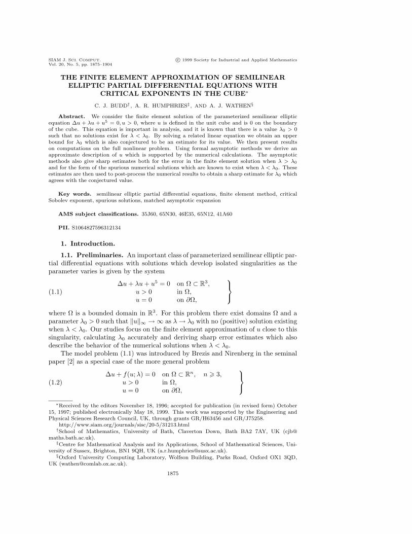
Fig. 1.1. Graph of ‖Uh‖∞ against λ, for grids varying between h = 1/60 and h = 1/100, with
λ0 indicated by the vertical line.
under mesh refinement and are almost indistinguishable from them if λ0 is unknown.Consequently, the range of existence of the true solutions is hard to determine.
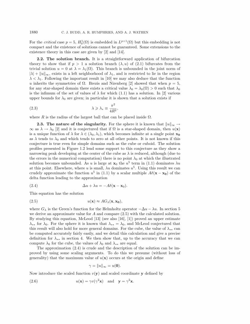
In Figure 1.1 we present a graph of the infinity norm of the discrete solution Uh
as a function of λ and also indicate a value of λ0 = 7.5045 which is conjectured fromfurther computations in this paper. This graph was obtained for a solution of (1.1) onthe unit cube 0 6 x, y, z 6 1 using the finite element method with piecewise trilinearbasis functions defined over cubes of side h = 1/60, . . . , 1/100. Observe that each ofthe curves looks smooth with no significant hint of singular behavior occurring closeto λ0.
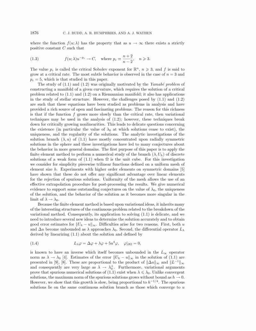
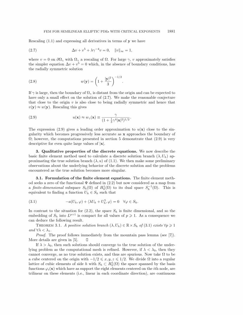
In Figure 1.2 we present a cross section of the resulting solution taken in the planez = 1/2 with h = 1/100 for λ = (a) 20, (b) 15, (c) 7.5045, (d) 0. In this graph figures(a) and (b) are approximations to true solutions, (d) is certainly spurious, and furthercomputations strongly imply that (c) is also spurious. From these figures we observethat each of these figures exhibits a peak forming in the center of the cube whichgrows as λ is reduced. Although the peak in (c) and (d) is higher than those in (a)and (b), its appearance does not appear to be significantly different (i.e., it appearswell resolved by the mesh) and it is very hard a priori to distinguish from numericalevidence alone between the true and spurious solutions.
As the singularity forms it is computationally impossible to use a fine enoughuniform mesh to resolve its structure, and indeed the employment of a fixed meshultimately leads to the spurious solutions. This suggests that an adaptive approachwhich places a higher density of mesh points close to the singularity should be taken.Such methods are hard to implement in three dimensions; moreover, they typicallymake use of an a priori or a posteriori estimate of the local truncation and these esti-mates are not sharp for (1.1) due to the unboundedness of ‖L−1
λ ‖∞. Some preliminarycomputations of radially symmetric solutions of (1.1) reported in [6] demonstrate that
1878 C. J. BUDD, A. R. HUMPHRIES, AND A. J. WATHEN
(c)
(a)
(d)
(b)-0.4 -0.2 0.0 0.2 0.4-0.4-0.20.00.20.40
2
4
6
8
10
12
-0.4 -0.2 0.0 0.2 0.4-0.4-0.20.00.20.40
2
4
6
8
10
12
-0.4 -0.2 0.0 0.2 0.4-0.4-0.20.00.20.40
2
4
6
8
10
12
-0.4 -0.2 0.0 0.2 0.4-0.4-0.20.00.20.40
2
4
6
8
10
12
Fig. 1.2. Cross section of the numerical solution Uh through center of cube with h = 1/100 and
adaptive methods based upon local truncation or a posteriori error estimates are notparticularly accurate and still admit spurious solutions. As a consequence, we adopta different approach here by looking at the solution on a uniform mesh and use formalasymptotic methods, scaling arguments, and an approximation result (in Lemma 6.1)to obtain sharp estimates of both the convergent and the spurious solutions. By usingsufficiently fine meshes these estimates are descriptive and can be used to post-processthe numerical solution to give a much more accurate solution of (1.1) and an estimateof λ0. We show that if λ is close to but greater than λ0, then there is a constant Csuch that if h is sufficiently small (in particular if h2‖Uh‖8
∞ is small), then∣
∣‖u‖∞ − ‖Uh‖∞∣
∣
‖Uh‖∞≈ Ch2‖Uh‖8
∞2λ
.(1.5)
Observe the rapid growth in this estimate as ‖Uh‖∞ increases. If h satisfies the lessrestrictive requirement that h2‖Uh‖4
∞ is small, then
‖u‖∞ ≈ ‖Uh‖∞√
1 − Ch2‖Uh‖8/λ,(1.6)
which reduces to (1.5) in the limit of small h. In contrast, if λ = λ0 so that thenumerical solution is spurious we have that
‖Uh‖∞ ≈(
λ0
C
)1/8
h−1/4(1.7)
so that ‖Uh‖∞ grows slowly as h decreases. The value of C depends upon the elementsused but not upon the domain and can be calculated a priori. Consequently, theseresults have immediate extensions to problems with more complex geometries.
FEM FOR SEMILINEAR ELLIPTIC PDEs WITH CRITICAL EXPONENTS 1879
Although the restriction that h2‖Uh‖4∞ be small means that we must use a moder-
ately fine mesh for these results to be sharp when ‖Uh‖∞ is large, the restriction is nottoo severe and we are able to perform computations with such meshes for which (1.6)is sharp. Using this formula we derive in section 7 a procedure for post-processingthe results to obtain a more accurate value for ‖u‖∞ and hence to estimate λ0. Thispost-processing can be applied to results for more complex domains and for moregeneral nonlinearities which grow at the critical rate. The post-processing procedureis much easier to apply and more effective than the use of adaptive methods, giv-ing accurate numerical approximations and rejecting spurious solutions while usingmeshes for which computations are feasible.
As an application of these methods we give computational evidence to support aconjecture made by McLeod [13] that λ0 is equal to a value λ∗∗ obtained by solving arelated linear problem. (This is the value of λ indicated in Figure 1.1.) We also givestrong evidence to show that the solutions in the cube are unique and have a highdegree of radial symmetry away from the boundary.
The layout of the remainder of this paper is as follows. In section 2 we give a briefsummary of the significant analytic results and conjectures concerning (1.1) and inparticular describe the form of the developing singularity. In section 3 we derive thefinite element method and state some known results on its convergence. In section 4we apply this method to solve a linear problem which approximates (1.1) when u islarge. This gives both an upper bound and an estimate λ∗∗ for λ0. In section 5 wecompute solutions for the full problem (1.1) and present the results, indicating thatfor sufficiently fine meshes the solutions obey a scaling law. In section 6 we applyformal asymptotic techniques to derive an improved description of both u and Uh.Finally, in section 7, we use the asymptotic formula to derive the estimates (1.5),(1.6), (1.7) and then apply (1.6) to post-process the numerical results to obtain amore accurate description of the solution.
2. The qualitative form of the analytic solution branch.
2.1. Existence. We define bilinear operators a(u, v) and 〈u, v〉 by
a(u, v) =
∫
Ω
∇u.∇v dΩ and 〈u, v〉 =
∫
Ω
uv dΩ
and denote by H10 (Ω) the usual Sobolev space of functions vanishing on the boundary
of Ω with norm defined by ‖u‖2H1
0
= a(u, u). Furthermore, let λ1(Ω) be the small-
est eigenvalue, with positive eigenfunction vanishing on the boundary of Ω, of thedifferential operator −∆. A weak solution u ∈ H1
0 (Ω) of the general problem
∆u+ λu+ up = 0 on Ω ⊂ R3,
u > 0 in Ω,u = 0 on ∂Ω
(2.1)
is a zero of the function Ψ : H10 (Ω) → H−1(Ω) defined by
Ψ(u)ϕ = −a(u, ϕ) + 〈λu+ up, ϕ〉.(2.2)
If λ < λ1, then a sufficient condition (see, for example, [7]) for the existence of such a(nontrivial) weak solution is that H1
0 (Ω) is compactly embedded in Lp+1(Ω). For thesubcritical case p < 5, this condition holds and the variational approach predicts thatsolutions of (1.1) exist for all λ < λ1. The theory for this case is reviewed in Lions [11].
1880 C. J. BUDD, A. R. HUMPHRIES, AND A. J. WATHEN
For the critical case p = 5, H10 (Ω) is embedded in Lp+1(Ω) but this embedding is not
compact and the existence of solutions cannot be guaranteed. Some extensions to theexistence theory in this case are given by [2] and [14].
2.2. The solution branch. It is a straightforward application of bifurcationtheory to show that if p > 1 a solution branch (λ, u) of (2.1) bifurcates from thetrivial solution u = 0 at λ = λ1(Ω). This branch is unbounded in the joint norm of|λ| + ‖u‖∞, exists in a left neighborhood of λ1, and is restricted to lie in the regionλ < λ1. Following the important result in [10] we may also deduce that the functionu inherits the symmetries of Ω. Brezis and Nirenberg [2] showed that when p = 5,for any star-shaped domain there exists a critical value λ0 = λ0(Ω) > 0 such that λ0
is the infimum of the set of values of λ for which (1.1) has a solution. In [2] variousupper bounds for λ0 are given; in particular it is shown that a solution exists if
λ > λ∗ ≡ π2
4R2,(2.3)
where R is the radius of the largest ball that can be placed inside Ω.
2.3. The nature of the singularity. For the sphere it is known that ‖u‖∞ →∞ as λ → λ0 [2] and it is conjectured that if Ω is a star-shaped domain, then u(x)is a unique function of λ for λ ∈ (λ0, λ1), which becomes infinite at a single point x0
as λ tends to λ0 and which tends to zero at all other points. It is not known if thisconjecture is true even for simple domains such as the cube or cuboid. The solutionprofiles presented in Figure 1.2 lend some support to this conjecture as they show anarrowing peak developing at the center of the cube as λ is reduced, although (due tothe errors in the numerical computation) there is no point λ0 at which the illustratedsolution becomes unbounded. As u is large at x0 the u5 term in (1.1) dominates λuat this point. Elsewhere, where u is small, λu dominates u5. Using this result we cancrudely approximate the function u5 in (1.1) by a scalar multiple Aδ(x − x0) of thedelta function leading to the approximation
∆u+ λu = −Aδ(x − x0).(2.4)
This equation has the solution
u(x) ≈ AGλ(x,x0),(2.5)
where Gλ is the Green’s function for the Helmholtz operator −∆u− λu. In section 5we derive an approximate value for A and compare (2.5) with the calculated solution.By studying this equation, McLeod [13] (see also [16], [1]) proved an upper estimateλ∗∗ for λ0. For the sphere it is known that λ∗∗ = λ0, and McLeod conjectured thatthis result will also hold for more general domains. For the cube, the value of λ∗∗ canbe computed accurately fairly easily, and we detail this calculation and give a precisedefinition for λ∗∗ in section 4. We then show that, up to the accuracy that we cancompute λ0 for the cube, the values of λ0 and λ∗∗ are equal.
The approximation (2.4) is crude and the description of the solution can be im-proved by using some scaling arguments. To do this we presume (without loss ofgenerality) that the maximum value of u(x) occurs at the origin and define
γ = ‖u‖∞ = u(0).
Now introduce the scaled function v(y) and scaled coordinate y defined by
u(x) = γv(γ2x) and y = γ2x.(2.6)
FEM FOR SEMILINEAR ELLIPTIC PDEs WITH CRITICAL EXPONENTS 1881
Rescaling (1.1) and expressing all derivatives in terms of y we have
∆v + v5 + λγ−4v = 0, ‖v‖∞ = 1,(2.7)
where v = 0 on ∂Ωγ with Ωγ a rescaling of Ω. For large γ, v approximately satisfiesthe simpler equation ∆v + v5 = 0 which, in the absence of boundary conditions, hasthe radially symmetric solution
w(y) =
(
1 +|y|23
)−1/2
.(2.8)
If γ is large, then the boundary of Ωγ is distant from the origin and can be expected tohave only a small effect on the solution of (2.7). We make the reasonable conjecturethat close to the origin v is also close to being radially symmetric and hence thatv(y) ≈ w(y). Rescaling this gives
u(x) ≈ wγ(x) ≡ γ
(1 + 13γ
4|x|2)1/2 .(2.9)
The expression (2.9) gives a leading order approximation to u(x) close to the sin-gularity which becomes progressively less accurate as x approaches the boundary ofΩ; however, the computations presented in section 5 demonstrate that (2.9) is verydescriptive for even quite large values of |x|.
3. Qualitative properties of the discrete equations. We now describe thebasic finite element method used to calculate a discrete solution branch (λ,Uh) ap-proximating the true solution branch (λ, u) of (1.1). We then make some preliminaryobservations about the underlying behavior of the discrete solution and the problemsencountered as the true solution becomes more singular.
3.1. Formulation of the finite element equations. The finite element meth-od seeks a zero of the functional Ψ defined in (2.2) but now considered as a map froma finite-dimensional subspace Sh(Ω) of H1
0 (Ω) to its dual space S−1h (Ω). This is
equivalent to finding a function Uh ∈ Sh such that
−a(Uh, ϕ) + 〈λUh + U5h , ϕ〉 = 0 ∀ϕ ∈ Sh.(3.1)
In contrast to the situation for (2.2), the space Sh is finite dimensional, and so theembedding of Sh into Lp+1 is compact for all values of p > 1. As a consequence wecan deduce the following result.
Theorem 3.1. A positive solution branch (λ,Uh) ∈ R×Sh of (3.1) exists ∀p > 1and ∀λ < λ1.
Proof. The proof follows immediately from the mountain pass lemma (see [7]).More details are given in [5].
If λ > λ0, then such solutions should converge to the true solution of the under-lying problem as the computational mesh is refined. However, if λ < λ0, then theycannot converge, as no true solution exists, and thus are spurious. Now take Ω to bea cube centered on the origin with −1/2 6 x, y, z 6 1/2. We divide Ω into a regularlattice of cubic elements of side h with Sh ⊂ H1
0 (Ω) the space spanned by the basisfunctions ϕi(x) which have as support the eight elements centered on the ith node, aretrilinear on these elements (i.e., linear in each coordinate direction), are continuous
1882 C. J. BUDD, A. R. HUMPHRIES, AND A. J. WATHEN
across the element boundaries, take the value 1 at the ith node, and are zero at allother nodes. Thus we may represent Uh(x) as
For this calculation, the simple polynomial nature of the nonlinearity means thatall integrals can be evaluated exactly by using Gaussian quadrature on each elementwith four integration points in each coordinate direction. The finite element methodthus reduces the problem (3.1) to solving N coupled (nonlinear) equations for theunknowns U = [U1, . . . , Un]T ∈ R
n and we rewrite (3.2) as
KU = λAU + G(U),(3.3)
where Kij = a(ϕi, ϕj), Aij = 〈ϕi, ϕj〉, and [G(U)]i = 〈U5h , ϕi〉. By solving (3.3) we
can thus find a branch (λ,Uh) of solutions of the discrete weak equation (3.1). Thearguments presented in [15] show that the branch so computed satisfies
‖Uh‖∞ < Ch−1/2,
where C depends upon the domain, but not on λ, h, or Uh.As will be clear in section 5, it is necessary to take N ≈ 106 nodes, which leads
to severe computational difficulties in solving the algebraic systems. Our techniquefor finding the solution is to exploit the natural homotopy parameter λ and solve(3.3) by numerical continuation in this parameter given a suitable starting point, andmaking small reductions in λ at each step. For each such step we solve (3.3) by usinga pseudo-Newton method for which the Jacobian of the problem is approximated bya related matrix with reduced memory allocation. These pseudo-Jacobian matricesare symmetric but not positive definite. The resulting linear systems are then solvedby using the conjugate gradient method without preconditioning. There are two rea-sons why preconditioning is not used. First, standard preconditioners are ineffectivebecause the pseudo-Jacobian matrices are not positive definite, and second, the un-conditioned method converges relatively quickly. For an unpreconditioned system ifthe indefiniteness causes difficulties with the convergence of the conjugate gradient(CG) method, then this is readily seen. Although CG is robust only for positive defi-nite systems, we found no convergence difficulties for our (mildly) indefinite problems.For example, on a mesh of 1003 = 106 elements making a step of ∆λ = 0.5 betweensuccessive values of λ, on average only 1.32 iterations of the Newton method and 210inner iterations of the CG method are needed to obtain a convergent solution at eachstep.
3.2. Starting the branch. An application of standard bifurcation theory tothe discrete problem (3.3) implies that there is a bifurcation of a nontrivial solutionbranch from the zero solution at the value λ = λ1, h, where λ1, h is the smallestgeneralized eigenvalue of the system linearized about U = 0 satisfying
Kψ1, h = λAψ1, h
FEM FOR SEMILINEAR ELLIPTIC PDEs WITH CRITICAL EXPONENTS 1883
with a nonzero vector ψ1, h. This equation is a discretization of the Helmholtz equation−∆ψ1 = λψ1, ψ = 0 if x ∈ ∂Ω satisfied (for nonzero ψ) when λ = λ1(Ω) and fromstandard results in approximation theory we have that λ1 < λ1, h = λ1 + O(h2). Forthe unit cube λ1 = 3π2 and
ψ1(x) = ψ1(x, y, z) = cos(πx) cos(πy) cos(πz).
Taking λ = λ1 initially and setting Uh = ψ1 with ψ1 the interpolant of ψ1 in Sh proveda sufficiently accurate initial guess to allow rapid convergence onto the solution branch.
3.3. Convergence of the numerical method. The study of the convergenceof the discretizations of general semilinear equations is not new. An overall theory(based upon the implicit function theorem or on concepts of nonlinear stability) hasbeen developed for the numerical approximation of isolated solutions of problemsof the form (1.1) for fairly general functions f(u;λ). Good references to this workare given in the monograph by Crouzeix and Rappaz [8] and also in the papers byLopez-Marcos and Sanz-Serna [12] and Dobrowolski and Rannacher [9]. Such resultstypically assume that a solution Uh has been constructed in a neighborhood of thetrue solution u and look at the convergence of Uh to u as the mesh is refined. Forpiecewise linear finite elements, we have [9]
‖Uh − u‖∞ < B∞(u)h2 log(1/h), ‖Uh − u‖H1
0
< BH(u)h as h→ 0.(3.4)
In Lopez-Marcos and Sanz-Serna [12] it is also shown that there exist neighborhoodsof u (called stability balls) in which Uh both exists and is unique. In Murdoch andBudd [15] these results were applied directly to problems of the form (1.1) and it wasshown that the radii of the stability balls were mesh dependent and that spurioussolutions could exist outside them. For the estimates of ‖Uh − u‖∞ the constantB∞(u) is proportional both to ‖∆u‖∞ = ‖λu+ u5‖∞ and to the infinity norm of theoperator L−1
λ defined in (1.4). Because both are unbounded as λ → λ0 the aboveestimate is hard to apply, and descriptive only when h is very small. Consequently,the result (3.4) does not give a completely satisfactory account of the convergence ofa numerical method for (1.1).
3.4. Spurious solutions of the numerical method. A secondary difficultyarises with spurious solutions when λ < λ0. Obviously, it is important to distinguishsuch solutions from convergent approximations to solutions of (1.1). In particular,they diverge to infinity in L∞(Ω) as the mesh is refined but remain bounded inother norms. Indeed, we observe spurious solutions of (1.1) which remain boundedin H1
0 (Ω) under mesh refinement and tend to zero in L2(Ω). As mentioned in theintroduction, the divergence in L∞ as the mesh is refined can be very slow; typicallyfor spurious solutions of (1.1) we will see that ‖Uh‖∞ ∼ h−1/4 ∼ N1/12 where Nis the number of computational nodes. With such a slow rate of divergence it isnot computationally feasible to use fine enough meshes to clearly distinguish betweena slowly growing spurious solution and a convergent solution. This motivates thecalculations in section 6 where asymptotic methods are used to distinguish betweenthe two types of solution.
3.5. Resolution of the singularity. The main difficulty posed to the numericalmethod is an adequate resolution of the singularity as λ → λ0. A preliminary erroranalysis can be made by considering the rescaling (2.6) which can also be applied tothe finite element discretization. In particular, suppose that
γ = ‖Uh‖∞, y = γ2x and Uh(x) = γVH(γ2x),(3.5)
1884 C. J. BUDD, A. R. HUMPHRIES, AND A. J. WATHEN
where
H = γ2h.(3.6)
Under this rescaling VH(y) belongs to the space of functions spanned by piecewisetrilinear basis functions defined on cubes of side H. In the rescaled variables, we haveconjectured that close to its peak the rescaled function v(y) has the approximate form
v(y) ≈ 1/(1 + |y|2/3)1/2.
For VH to approximate this function it is clearly necessary thatH 1. Standard errorestimates then imply that we can approximate v(y) to an accuracy of O(H2) by usingpiecewise linear elements and hence, on the original mesh, we can approximate therescaled function wγ(x) to an accuracy of O(h2γ5). Thus, a necessary condition foran accurate numerical solution of (1.1) is that H is small. Now observe that whereash is known, the value of H can only be determined subsequent to the computation.Moreover, the condition of H being small is not sufficient since we have no a prioriguarantee that the value of γ itself is correct. Thus, although the numerical methodmay be able to resolve the profile of the singularity, it may get its maximum valuewrong. This turns out to be a second principal source of error, and we return to thisin sections 5 and 6.
4. Critical values of λ derived from the linear Green’s function.
4.1. McLeod’s conjecture. For our first investigations of the solutions of thenonlinear partial differential equation problem (1.1) we study the solutions of therelated linear problem (2.4) approximating (1.1) when u is large. A numerical studyof this problem is rather simpler than that for (1.1) and yet gives insight into thebehavior of the large solutions and affords the possibility of determining the range ofexistence of the solutions of (1.1) without solving the fully nonlinear problem.
For general x, y the Green’s function for the Helmholtz operator satisfies theequation
∆Gλ(x,y) + λGλ(x,y) = −δ(x − y), x ∈ Ω,Gλ(x,y) = 0, x ∈ ∂Ω
(4.1)
(where all spatial derivatives are expressed in terms of x). Since
∆
(
1
4π|x − y|
)
= −δ(x − y)(4.2)
we may write
Gλ(x,y) =1
4π|x − y| + gλ(x,y),(4.3)
where the continuous but nonsmooth function gλ(x,y) is called the regular part ofthe Green’s function. It follows from (4.1) and (4.3) that
∆gλ(x,y) + λgλ(x,y) = − λ
4π|x − y| , x ∈ Ω,
gλ(x,y) = − 1
4π|x − y| , x ∈ ∂Ω.
(4.4)
FEM FOR SEMILINEAR ELLIPTIC PDEs WITH CRITICAL EXPONENTS 1885
Following Brezis [1] we define the function ϕλ(x) ≡ gλ(x,x). McLeod [13] and Schoen[16] showed independently that if ϕλ(x) > 0 for some point x in Ω, then (1.1) has asolution. In [1] it is shown that ϕλ(x) increases with λ and hence there is a uniqueλ = λ∗∗ and an x0 ∈ Ω, such that
max(ϕλ(x):x ∈ Ω) = ϕλ(x0) = 0 if λ = λ∗∗.
Hence we have the following result.Lemma 4.1. The problem (1.1) has a solution if λ > λ∗∗.McLeod conjectured that λ∗∗ = λ0. Strong numerical evidence supporting this
conjecture is presented in the rest of this paper.It is clear from the discussion above that a numerical computation of the function
gλ(x,y) and hence of ϕλ(x) has the potential of giving much insight into the solutionsof (1.1). This computation requires the solution of a linear problem, which can bedetermined with great accuracy at relatively little cost. In cuboid domains centered onthe origin, symmetry arguments imply that x0 = 0 and hence we need only computeϕλ(0).
Equation (4.4) has a singularity as |x − y| → 0 making computation difficult.Consequently, we solve a related problem which removes this singularity. In contrastto (4.3) we write
Gλ(x,y) = θλ(x,y) + hλ(x,y), where θλ(x,y) =cos(λ1/2|x − y|)
4π|x − y| .(4.5)
A simple calculation shows that
∆θλ(x,y) + λθλ(x,y) = −δ(x − y),(4.6)
and substituting (4.5) into (4.1) and using (4.6) we obtain
∆hλ(x,y) + λhλ(x,y) = 0, x ∈ Ω,hλ(x,y) = −θλ(x,y), x ∈ ∂Ω.
(4.7)
If y /∈ ∂Ω, then the function θλ is smooth on the boundary of ∂Ω. Thus, if λ < λ1,standard results from the theory of elliptic partial differential equations predict thatthe function hλ exists and is smooth in the interior of Ω. Finally, using (4.3) and (4.5)it follows that
gλ(x,y) =1
4π|x − y|(
cos(λ1/2|x − y|) − 1)
+ hλ(x,y).(4.8)
To compute λ∗∗ for cuboid domains with x0 = 0 we solve (4.7) for hλ(x, 0) usingthe finite element method with the same mesh and basis functions as in section 3.Letting x → 0 in (4.8) then gives
ϕλ(0) = gλ(0,0) = hλ(0,0).(4.9)
The value of λ∗∗ is determined by using path following in λ and interval bisectionto find the unique value for which ϕλ∗∗
(0) = 0. We note that as the function hλ issmooth, then standard error estimates of the form (3.4) from the theory of the finiteelement method may be applied to estimate the accuracy of the above computation.As the value of θλ on ∂Ω depends smoothly upon λ, as does the inverse of the linearoperator in (4.8), the constants implied in these calculations (unlike those in thecalculation of the nonlinear equation) are largely independent of λ, and consequentlywe predict a consistently accurate solution.
1886 C. J. BUDD, A. R. HUMPHRIES, AND A. J. WATHEN
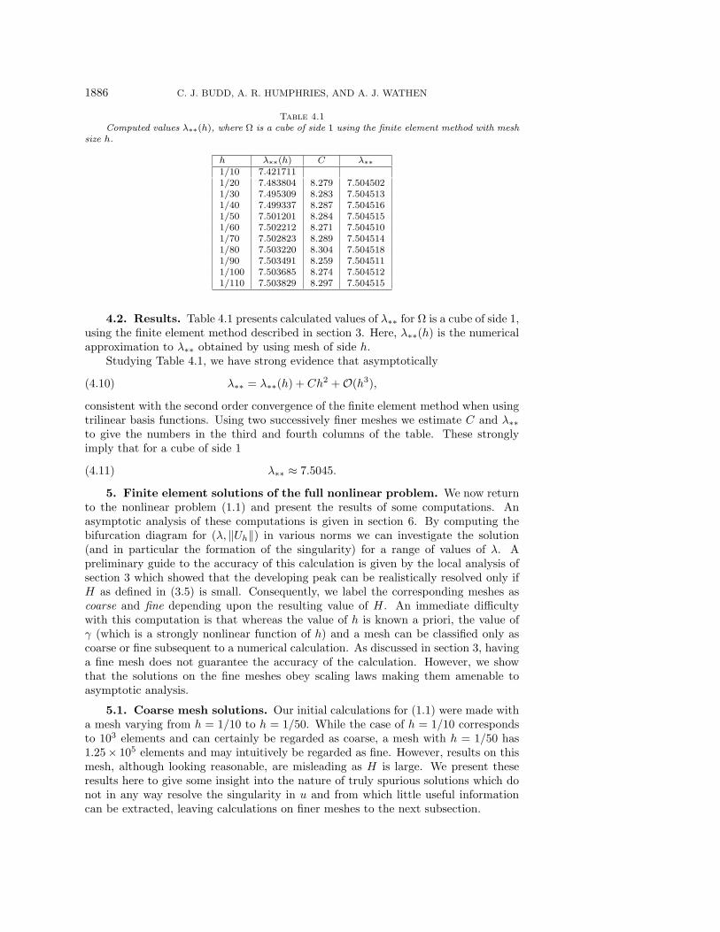
Table 4.1
Computed values λ∗∗(h), where Ω is a cube of side 1 using the finite element method with mesh
4.2. Results. Table 4.1 presents calculated values of λ∗∗ for Ω is a cube of side 1,using the finite element method described in section 3. Here, λ∗∗(h) is the numericalapproximation to λ∗∗ obtained by using mesh of side h.
Studying Table 4.1, we have strong evidence that asymptotically
λ∗∗ = λ∗∗(h) + Ch2 + O(h3),(4.10)
consistent with the second order convergence of the finite element method when usingtrilinear basis functions. Using two successively finer meshes we estimate C and λ∗∗to give the numbers in the third and fourth columns of the table. These stronglyimply that for a cube of side 1
λ∗∗ ≈ 7.5045.(4.11)
5. Finite element solutions of the full nonlinear problem. We now returnto the nonlinear problem (1.1) and present the results of some computations. Anasymptotic analysis of these computations is given in section 6. By computing thebifurcation diagram for (λ, ‖Uh‖) in various norms we can investigate the solution(and in particular the formation of the singularity) for a range of values of λ. Apreliminary guide to the accuracy of this calculation is given by the local analysis ofsection 3 which showed that the developing peak can be realistically resolved only ifH as defined in (3.5) is small. Consequently, we label the corresponding meshes ascoarse and fine depending upon the resulting value of H. An immediate difficultywith this computation is that whereas the value of h is known a priori, the value ofγ (which is a strongly nonlinear function of h) and a mesh can be classified only ascoarse or fine subsequent to a numerical calculation. As discussed in section 3, havinga fine mesh does not guarantee the accuracy of the calculation. However, we showthat the solutions on the fine meshes obey scaling laws making them amenable toasymptotic analysis.
5.1. Coarse mesh solutions. Our initial calculations for (1.1) were made witha mesh varying from h = 1/10 to h = 1/50. While the case of h = 1/10 correspondsto 103 elements and can certainly be regarded as coarse, a mesh with h = 1/50 has1.25× 105 elements and may intuitively be regarded as fine. However, results on thismesh, although looking reasonable, are misleading as H is large. We present theseresults here to give some insight into the nature of truly spurious solutions which donot in any way resolve the singularity in u and from which little useful informationcan be extracted, leaving calculations on finer meshes to the next subsection.
FEM FOR SEMILINEAR ELLIPTIC PDEs WITH CRITICAL EXPONENTS 1887
0 10 20 300
5
10
15
λ
‖Uh‖∞
10
20
30
40
50
Fig. 5.1. Bifurcation diagram of ‖Uh‖∞ against λ for coarse grids varying between h = 1/10and h = 1/50.
From Figure 5.1 it is evident that a solution branch of the numerical discretizationexists for all λ < λ1. A steep gradient forms in each figure and the value of λ at whichthis occurs decreases as the mesh is refined. This gives the misleading picture thatλ0 is close to zero. However, we observe that as the mesh is refined, there is littleagreement among any of the curves when λ 6 13 and the structures observed for thisrange of λ should be viewed with suspicion. A qualitative indication of this is thenonmonotonicity of the graph of ‖Uh‖∞ under mesh refinement, leading to a braidingstructure in the bifurcation diagram.
A useful measure of the error of the solution is given by the value of H whenλ = λ∗∗. In particular we have H = 4.914 if h = 1/10 and H = 1.157 if h = 1/50.
5.2. Bifurcation diagrams for the fine mesh solutions in various norms.
We now look at computations on finer meshes for which H takes smaller values thanpreviously and for which the results obey a detectable asymptotic scaling law as h→ 0.
5.2.1. The maximum norm. A plot of ‖Uh‖∞ against λ for values of themesh size from h = /60 to h = 1/100 (106 elements) was presented in Figure 1.1. Thesolution branches for all these meshes agree for λ ' 12, and for smaller values of λthis figure is strikingly different from Figure 5.1. Excepting the case of the h = 1/60branch near λ = 0, we see that the value of ‖Uh‖∞ is monotonically increasing asthe mesh is refined, avoiding the braiding seen earlier. In this case the value ofH when λ = λ∗∗ decreases from H = 1.032 when h = 1/60 to H = 0.774 whenh = 1/100. Although this value is still not very small, it appears to be small enoughfor the asymptotic theory we will develop to be descriptive. It is revealing to also plot1/‖Uh‖2
∞. This is given in Figure 5.2.
For the sphere it is shown in [4], [3] that 1/‖u‖2∞ is proportional to λ − λ0 if
λ is close to λ0. In Figure 5.2 we see that the corresponding curve for 1/‖Uh‖2∞ in
1888 C. J. BUDD, A. R. HUMPHRIES, AND A. J. WATHEN
0 5 10 150.00
0.02
0.04
0.06
Fig. 5.2. Bifurcation diagram of 1/‖Uh‖2∞ against λ for grids varying between h = 1/60 and
h = 1/100. For moderate values of λ (λ ∈ [5, 10]) the value of 1/‖Uh‖2∞ decreases monotonically as
the mesh is refined.
Table 5.1
Computed values of ‖Uh‖∞ for various values of λ and various mesh sizes.
the cube is approximately linear for 12 < λ < 15 but departs from linearity as λ isreduced. Extrapolating the linear section gives an intercept (indicated) at a value ofλ close to λ∗∗. In section 7 we will demonstrate much stronger reasons for believingthat λ0 = λ∗∗. In Table 5.1 we present a table of ‖Uh‖∞ for various values of λbetween 0 and 10, with mesh sizes between h = 1/10 and h = 1/100. For any fixedvalue of λ in the table the value of ‖Uh‖∞ is ultimately monotonically increasing asthe mesh is refined; however, the smaller the value of λ, the finer the mesh must betaken before this monotonicity is observed and any scaling law becomes apparent.
Table 5.1 clearly indicates the difficulties in determining the difference betweena convergent and a spurious solution. For λ > λ∗∗ = 7.5045, Lemma 4.1 gives theexistence of a solution of (1.1) and consequently Uh will converge toward this solutionas h→ 0. However, it is almost impossible from an a priori inspection to differentiate
FEM FOR SEMILINEAR ELLIPTIC PDEs WITH CRITICAL EXPONENTS 1889
0.00 0.02 0.04 0.06 0.08 0.104
6
8
10
12
67
89
10
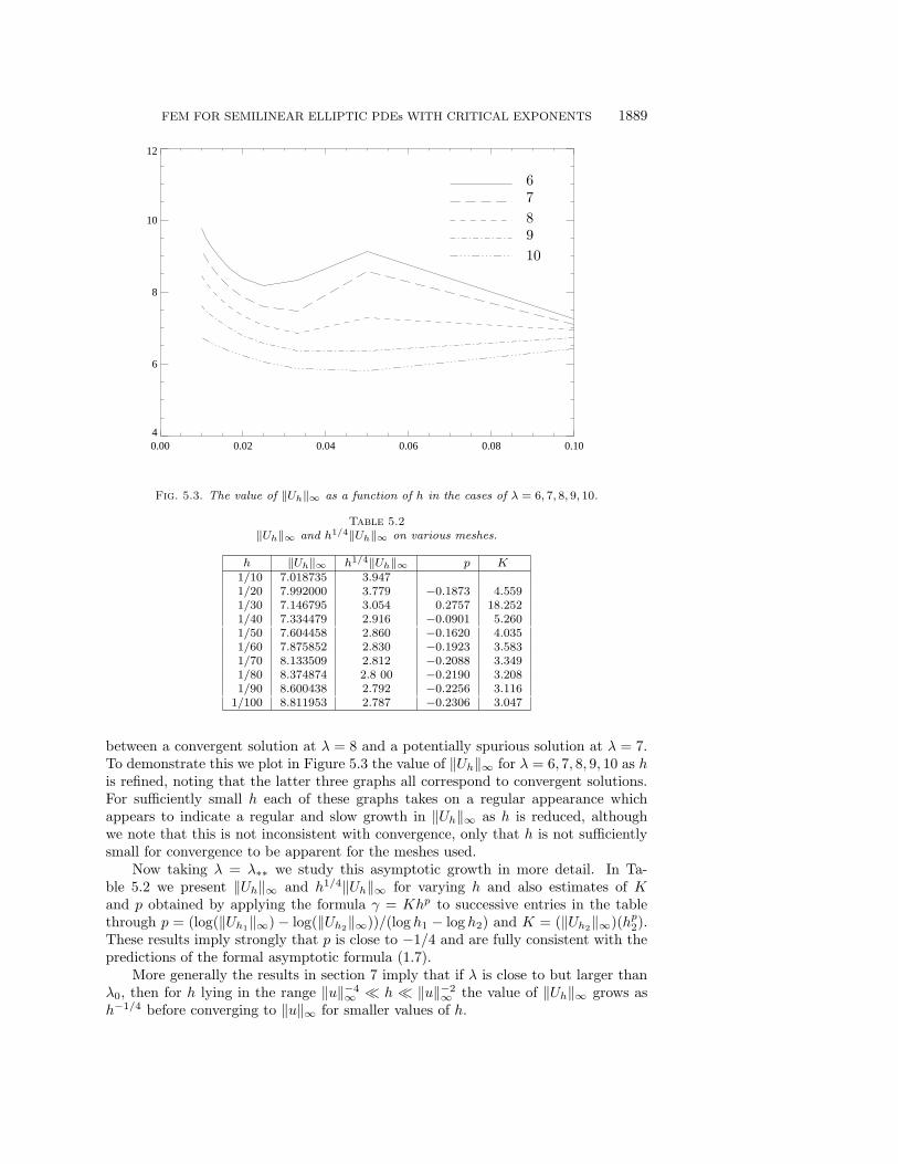
Fig. 5.3. The value of ‖Uh‖∞ as a function of h in the cases of λ = 6, 7, 8, 9, 10.
between a convergent solution at λ = 8 and a potentially spurious solution at λ = 7.To demonstrate this we plot in Figure 5.3 the value of ‖Uh‖∞ for λ = 6, 7, 8, 9, 10 as his refined, noting that the latter three graphs all correspond to convergent solutions.For sufficiently small h each of these graphs takes on a regular appearance whichappears to indicate a regular and slow growth in ‖Uh‖∞ as h is reduced, althoughwe note that this is not inconsistent with convergence, only that h is not sufficientlysmall for convergence to be apparent for the meshes used.
Now taking λ = λ∗∗ we study this asymptotic growth in more detail. In Ta-ble 5.2 we present ‖Uh‖∞ and h1/4‖Uh‖∞ for varying h and also estimates of Kand p obtained by applying the formula γ = Khp to successive entries in the tablethrough p = (log(‖Uh1
‖∞) − log(‖Uh2‖∞))/(log h1 − log h2) and K = (‖Uh2
‖∞)(hp2).These results imply strongly that p is close to −1/4 and are fully consistent with thepredictions of the formal asymptotic formula (1.7).
More generally the results in section 7 imply that if λ is close to but larger thanλ0, then for h lying in the range ‖u‖−4
∞ h ‖u‖−2∞ the value of ‖Uh‖∞ grows as
h−1/4 before converging to ‖u‖∞ for smaller values of h.
1890 C. J. BUDD, A. R. HUMPHRIES, AND A. J. WATHEN
0 10 20 300
1
2
3
4
5
Fig. 5.4. Bifurcation diagram of ‖Uh‖H1
0
against λ, for grids varying between h = 1/10 and
h = 1/100. The value of ‖Uh‖H1
0
is monotonically decreasing as the mesh is refined.
5.2.2. The Sobolev norm. In Figure 5.4 we display the solution branches inthe H1
0 (Ω) norm. We note from this figure that the values of ‖Uh‖H1
0
appear to
converge (to a value between 3.5 and 4) as h → 0. Also away from the bifurcationpoint ‖Uh‖H1
0
is roughly constant as λ is varied, although its maximum norm γ is
changing. Observe that if wγ(x) is defined as in (2.9), then
‖wγ‖H1(R3) =33/4π
2= 3.58063,(5.1)
which is both independent of γ and close to the converged value. As the greatestcontribution to the Sobolev norm of both u and of wγ comes from the contributiondue to the peak, this result is consistent with the conjecture made in section 2 thatin the peak u is closely approximated by wγ .
5.3. The form of the solution. From the calculations on the fine meshes wemay draw some preliminary conclusions as to the form of the solution, in particularevidence for uniqueness, singularity, and symmetry. We summarize these here.
5.3.1. Uniqueness. An initial, simple, but important observation for the cube isthat the solution branch bifurcates monotonically to the left, so that ‖Uh‖∞ increasesas λ decreases. In particular, there are no fold bifurcations or transcritical bifurcationson the branch and the solutions on the main branch appear to be unique for all valuesof λ < λ1. All attempts to find additional solutions by starting from a point fardistant from the main branch failed to give anything new. Accordingly, we make theconjecture that the solutions of (1.1) are unique in cuboid domains.
5.3.2. The behavior close to the peak. In section 2 we discussed two de-scriptions of the approximation, namely, approximating u5 by a delta function and
FEM FOR SEMILINEAR ELLIPTIC PDEs WITH CRITICAL EXPONENTS 1891
0.0 0.2 0.4 0.6 0.8 1.00
2
4
6
8
10
Uh.
4π√
3
γGλ∗∗
(x, 0).
wγ .
•
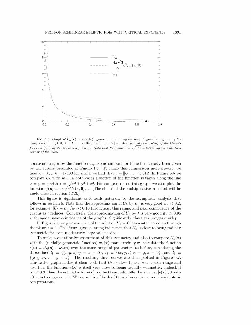
Fig. 5.5. Graph of Uh(x) and wγ(r) against r = |x| along the long diagonal x = y = z of the
cube, with h = 1/100, λ = λ∗∗ = 7.5045, and γ = ‖Uh‖∞. Also plotted is a scaling of the Green’s
function (4.3) of the linearized problem. Note that the point r =√
3/4 = 0.866 corresponds to a
corner of the cube.
approximating u by the function wγ . Some support for these has already been givenby the results presented in Figure 1.2. To make this comparison more precise, wetake λ = λ∗∗, h = 1/100 for which we find that γ ≡ ‖U‖∞ = 8.812. In Figure 5.5 wecompare Uh with wγ . In both cases a section of the function is taken along the line
x = y = z with r =√
x2 + y2 + z2. For comparison on this graph we also plot thefunction f(x) ≡ 4π
√3Gλ(x,0)/γ. (The choice of the multiplicative constant will be
made clear in section 5.3.3.)This figure is significant as it leads naturally to the asymptotic analysis that
follows in section 6. Note that the approximation of Uh by wγ is very good if r < 0.2,for example, |Uh −wγ |/wγ < 0.15 throughout this range, and near coincidence of thegraphs as r reduces. Conversely, the approximation of Uh by f is very good if r > 0.05with, again, near coincidence of the graphs. Significantly, these two ranges overlap.
In Figure 5.6 we give a section of the solution Uh with associated contours throughthe plane z = 0. This figure gives a strong indication that Uh is close to being radiallysymmetric for even moderately large values of x.
To make a quantitative assessment of this symmetry and also to compare Uh(x)with the (radially symmetric function) wγ(x) more carefully we calculate the functione(x) ≡ Uh(x) − wγ(x) over the same range of parameters as before, considering thethree lines l1 ≡ (x, y, z): y = z = 0, l2 ≡ (x, y, z):x = y, z = 0, and l3 ≡(x, y, z):x = y = z. The resulting three curves are then plotted in Figure 5.7.This latter graph makes it clear both that Uh is close to wγ over a wide range andalso that the function e(x) is itself very close to being radially symmetric. Indeed, if|x| < 0.3, then the estimates for e(x) on the three radii differ by at most |e(x)|/8 withoften better agreement. We make use of both of these observations in our asymptoticcomputations.
1892 C. J. BUDD, A. R. HUMPHRIES, AND A. J. WATHEN
-0.4-0.2
0.00.2
0.4
-0.4
-0.2
0.0
0.2
0.40
2
4
6
8
10
-0.4-0.2
0.00.2
0.4
-0.4
-0.2
0.0
0.2
0.4
Fig. 5.6. A cross section of Uh through center of cube with h = 1/100 and λ = λ∗∗ = 7.5045,with a contour plot which clearly shows the radial symmetry of the solution in the center of the
domain.
5.3.3. Behavior away from the peak. It is clear from Figure 5.5 that awayfrom the peak that Uh is close to 4π
√3Gλ/γ. This is consistent with the approximation
for u given in (2.4) for which we had u = AGλ(x,0). From section 4 we have that
Gλ(x,0) =1
4π|x| + gλ(x,0).(5.2)
Now if γ is large, γ2|x| is large, and |x| is small, then
wγ(x) ≈√
3
γ|x| and AGλ(x,0) ≈ A
4π|x| ,
so the two approximate descriptions of u agree to leading order if
A ≈ A1 ≡ 4π√
3
γ,
leading to the choice made in Figure 5.5. By making a small change to this result andtaking A = 1.012 × 4π
√3/γ, then the agreement is even better, with the functions
nearly coinciding. The reason for this small correction will be made evident in thenext section. A comparison is made in Figure 5.8 of the difference between these twofunctions in this case along the three radii taken before.
From this discussion we infer the following description of Uh if γ is large.• There is an (inner) region |x| < r1 such that Uh is close to the radially sym-
metric function wγ . Furthermore, the departure of Uh from radial symmetryis much smaller than the difference |Uh − wγ |.
• There is an (outer) region |x| > r2 such that u is close to AGλ for appropri-ate A.
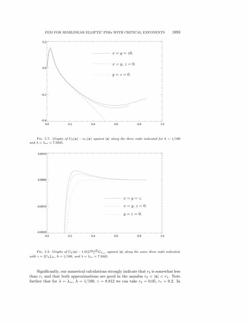
FEM FOR SEMILINEAR ELLIPTIC PDEs WITH CRITICAL EXPONENTS 1893
0.0 0.2 0.4 0.6 0.8 1.0-0.4
-0.2
0.0
0.2
x = y = z0.
x = y, z = 0.
y = z = 0.
Fig. 5.7. Graphs of Uh(x) − wγ(x) against |x| along the three radii indicated for h = 1/100and λ = λ∗∗ = 7.5045.
0.0 0.2 0.4 0.6 0.8 1.0-0.0020
-0.0010
0.0000
0.0010
x = y = z.
x = y, z = 0.
y = z = 0.
Fig. 5.8. Graphs of Uh(x) − 1.012 4π√
3γ
Gλ∗∗against |x| along the same three radii indicated,
with γ = ‖Uh‖∞, h = 1/100, and λ = λ∗∗ = 7.5045.
Significantly, our numerical calculations strongly indicate that r2 is somewhat lessthan r1 and that both approximations are good in the annulus r2 < |x| < r1. Notefurther that for λ = λ∗∗, h = 1/100, γ = 8.812 we can take r2 = 0.05, r1 = 0.2. In
1894 C. J. BUDD, A. R. HUMPHRIES, AND A. J. WATHEN
the rescaled variable y = γ2x we have γ2r2 = 3.87 and γ2r1 = 15.49, so that, whiler1 is small, in the rescaled variables the corresponding value is relatively large. Thisis important for the analysis in the next section.
6. Asymptotics of the discrete solution for large γ. Motivated by theabove calculations, we now develop a descriptive asymptotic theory. The results ofthe numerical calculations reported in the previous section have allowed us to drawsome preliminary conclusions about the form of the solutions of (1.1) but are imprecisedue to the relative coarseness of the discretization. To continue our discussion we nowmake a formal asymptotic calculation of the nature of the numerical discretization.This calculation then allows us to post-process the numerical results to obtain a moreaccurate picture of the form of the solution. This calculation extends those given in[15] and [5].
The principal errors in the numerical approximation occur when u is large and hasa large gradient. This occurs at the peak, precisely when u is well approximated bywγ with γ = ‖u‖∞. Our computations have also shown that the discrete function Uh
is close to wγ if now γ = ‖Uh‖∞. Thus we will proceed by calculating the differencebetween Uh and wγ and using this calculation to estimate ‖Uh‖∞. To obtain anasymptotic description of the piecewise linear function Uh we require a piecewiselinear approximation of wγ . A convenient such function is the interpolant Wγ, h(x)to wγ(x), which is the piecewise linear function coinciding with wγ(x) on the nodesof the mesh. Provided that H is small, the functions wγ and Wγ, h are close. Todo this we consider a representation of the function Uh(x) on an inner and an outerregion, such that on the inner region |x| is small and the function u is large and veryclose to being radially symmetric. Conversely, the outer region excludes the originbut extends to the boundary of Ω. These regions intersect in an annulus r1 < |x| < r2in which |x| is small but γ2|x| is large.
6.1. The inner region. We rescale the functions so that Uh(x) = γVH(γ2x),introduce the rescaled variable y = γ2x, and define Wγ, h(x) = γW1, H(γ2x), wherenow W1, H(y) is the piecewise linear interpolant of the function w1(y) on a uniformmesh of size H. Now, express the function VH(y) in an asymptotic series so that
VH(y) = V1, H(y) + γ−4V2, H(y) + · · · .
By construction, for each basis function ϕi(x) ∈ Sh, we have the identity
−a(Uh, ϕi) + λ〈Uh, ϕi〉 + 〈U5h , ϕi〉 = 0.
Suppose that ϕi,H(y) is defined to be ϕi(x) expressed on the rescaled mesh and thatall quadratures are now calculated with respect to y. We have
−a(VH , ϕi,H) +λ
γ4〈VH , ϕi,H〉 + 〈V 5
H , ϕi,H〉 = 0.
Substituting the asymptotic expression for VH into the above gives equations for V1, H ,V2, H , etc. For V1, H to satisfy the leading order equation exactly we would require
−a(V1, H , ϕi,H) + 〈V 51, H , ϕi,H〉 = 0.(6.1)
In fact, (6.1) has the solution w1(y) given in (2.9), but this function is not piecewiselinear. Instead we take V1, H to be the interpolant W1, H and introduce a small
FEM FOR SEMILINEAR ELLIPTIC PDEs WITH CRITICAL EXPONENTS 1895
discretization error into the leading order expression, which enters into the calculationof the function V2, H . This error can be expressed in terms of a residual Ri, where
Ri ≡ −a(W1, H , ϕi,H) + 〈W 51, H , ϕi,H〉.
Subtracting the identity (6.1) satisfied by w1 gives
Ri = −a(W1, H − w1, ϕi,H) + 〈W 51, H − w5
1, ϕi,H〉.(6.2)
Now looking at the next term in the asymptotic expansion for VH and using (6.2)we have
−a(V2, H , ϕi,H) + 5〈W 41, HV2, H , ϕi,H〉 = −λ〈W1, H , ϕi,H〉 + γ4Ri.(6.3)
As w1(y) is a smooth function of y and, for small H, the function w1 is closelyapproximated by its interpolant W1, H , we can use results from interpolation theoryto estimate the magnitude of Ri. In particular we use the following result.
Lemma 6.1. Let u(x) ∈ C4(Ω) be an arbitrary function of x ∈ R3, UH its
piecewise linear interpolant on a uniform mesh of size H, and f(u) a differentiable
function of u. Now, consider an element E comprising eight adjacent cubes, each of
side H, centered on the origin x ≡ (x, y, z) = (0, 0, 0), with
ϕH(x) =
(
1 − |x|H
)(
1 − |y|H
)(
1 − |z|H
)
, x ∈ E , ϕH(x) = 0 otherwise
the standard basis function on this element. Then there are constants K1 and K2
independent of u and H, such that if H is sufficiently small, then
Proof. Suppose first that aE ≡ a(u− UH , ϕH) = ax+ ay + az, where
ax =
∫ H
z=−H
∫ H
y=−H
∫ H
x=−H
(ux − UH,x)ϕH, x dx dy dz,(6.7)
with similar expressions for ay and az. Using the expression for ϕH(x) and integrating(6.7) we have
ax =1
H
∫ H
z=−H
∫ H
y=−H
(
[u− UH ]0−H − [u− UH ]H0)
(
1 − |y|H
)(
1 − |z|H
)
dy dz
= − 1
H
∫ H
z=−H
∫ H
y=−H
(
(u(H, y, z) − UH(H, y, z)) − 2(u(0, y, z) − UH(0, y, z))
+ (u(−H, y, z) − UH(−H, y, z)))
(
1 − |y|H
)(
1 − |z|H
)
dy dz.(6.8)
1896 C. J. BUDD, A. R. HUMPHRIES, AND A. J. WATHEN
By the uniqueness and linearity of interpolation, it follows that if u is an odd functionof y or of z, then so is UH . In the identity (6.8) the integration of all such oddfunctions vanishes. Thus we presume that the functions u(H, y, z), etc., are even in yand z so that locally the function u has the expansion
where the implied constant in the orderH4 terms is bounded by a multiple of (|uyyyy|+|uyyzz| + |uzzzz| + O(H2)). From these point values we can calculate UH . This thengives
u(H, y, z) = p(H) + q(H)y2 + r(H)z2 + O(H4),
UH(H, y, z) = p(H) + q(H)Hy + r(H)Hz + O(H4),
so that
u(H, y, z) − UH(H, y, z) = q(H)y(y −H) + r(H)z(z −H) + O(H4).
Similar expressions apply when 0 6 y, z 6 H and x = 0 or x = −H. Thus, over theset 0 6 y, z 6 H the contribution to the integral in (6.8) is given by
− 1
2H
∫ H
0
∫ H
0
[
y(y −H)(
uyy(H, 0, 0) − 2uyy(0, 0, 0) + uyy(−H, 0, 0))
+ z(z −H)(
uzz(H, 0, 0) − 2uzz(0, 0, 0) + uzz(−H, 0, 0))
+ O(H4)]
(
1 − y
H
)(
1 − z
H
)
dy dz
= − 1
2H
∫ H
0
∫ H
0
[
y(y −H)(
H2uyyxx(0, 0, 0) + O(H4))
+ z(z −H)(
H2uzzxx(0, 0, 0) + O(H4))
+ O(H4)]
(
1 − y
H
)(
1 − z
H
)
dy dz
= O(H5).
FEM FOR SEMILINEAR ELLIPTIC PDEs WITH CRITICAL EXPONENTS 1897
Here the implied constant in the order term is bounded by a multiple of (|uyyxx| +|uzzxx|+ |uyyyy|+ |uyyzz|+ |uzzzz|+O(H2)). Repeating this argument for the differentranges of y and z and then for ay and az gives (6.5).
Now, let bE = |〈f(u) − f(UH), ϕH〉|. As u and UH are close if H is small, we canestimate this by b 6 maxE|fu(u)||u − UH |〈1, ϕH〉. Now, standard results frominterpolation theory imply that there is a constant K independent of u such that
maxE
|u− UH | < KH2 maxE
|uxx| + |uyy| + |uzz|.
As 〈1, ϕH〉 < 4H3, this gives bE < H5B with B defined in (6.6).Combining these expressions gives the result in the lemma.To apply this result to calculate Ri, we take u = w1, f(u) = u5 and note that the
choice of the origin as being the center of the element was quite arbitrary.Now we consider again (6.3). For large s= |y|, w1(y)≈
√3/s so that 〈W1, H ,
ϕi,H〉 = O(H3/s). Now the second derivatives of w1 vary as 1/s3, and the fourthderivatives as 1/s5. Suppose that we look at the value of Ri corresponding to anelement centered on y. We can thus estimate that the corresponding values of Ai andBi from (6.5), (6.6) to be
Ai <α
|y|5 , Bi <β
|y|7 ,(6.9)
where α and β are bounded independently of i. For this range we have 〈W1, H , ϕi,H〉 Ri provided that H3/s γ4H5/s5, which is satisfied if s4 γ4H2, i.e., if r h.Assuming this is the case (consistently with our numerical observations), we have thatto a very good approximation
−a(V2, H , ϕi,H) = −⟨
λ√
3
s, ϕi,H
⟩
.
This equation is the weak form of
∆v = −λ√
3
s,
which has the solution
v(s) =a
s+ b− λ
√3
2s.
For large y this solution is smooth and has small second derivative terms proportionalto 1/s3. The discrete solution is consequently a perturbation with discretization errorproportional to H2/s3. Hence there are constants aH , bH such that
V2, H(y) =
(
aH|y| + bH − λ
√3|y|2
)
(
1 + O(H2/|s|2))
.(6.10)
We use quadrature to estimate the value of the constant bH . A direct calculationshows that the function
ψ(y) ≡ (1 − |y|23 )
(1 + |y|23 )3/2
=∂wγ
∂γevaluated at γ = 1
1898 C. J. BUDD, A. R. HUMPHRIES, AND A. J. WATHEN
satisfies the partial differential equation
∆ψ + 5w41ψ = 0.
Set ΨH(y) to be the piecewise linear interpolant to the function ψ(y). Differentiating(6.3) with respect to γ we have that ∀ i
−a(ΨH , ϕi,H) + 〈5W 41, HΨH , ϕi,H〉 = γ3Ti.(6.11)
The exact expression for Ti is complex, but simple scaling arguments imply that thereexists a constant C such that |Ti| < C|Ri|. (See the more detailed calculation givenin [5].) We now calculate bH by using a discrete form of the divergence theorem.Consider a cube C ⊂ Ωγ aligned with the mesh, centered on the origin, and of side2S, where S is large and an integer multiple of H. Now introduce piecewise linearfunctions ΨH and V2, H which coincide with ΨH and V2, H at all mesh points interior
to C, but which are zero on the boundary of, and exterior to, C. As both the functionsΨH , V2, H are in the span of the set of functions ϕi,H , there exist V i, Ψi such that
V2, H =∑
V iϕi,H , ΨH =∑
Ψiϕi,H .
Taking a linear combination of (6.3) and (6.11) and subtracting give
−a(V2, H , ΨH) + 〈5W 41, HV2, H , ΨH〉 + a(ΨH , V2, H) − 〈5W 4
1, HΨH , V2, H〉= −λ〈W1, H , Ψ〉 + γ4
∑
ΨiRi(y) − γ3∑
V iTi(y).(6.12)
The left-hand side of (6.12) has two contributions given by
a(ΨH , V2, H) − a(V2, H , ΨH) ≡ a(ΨH − ΨH , V2, H) − a(V2, H − V2, H ,ΨH)(6.13)
and
5(
〈W 41, HV2, H , ΨH〉 − 〈W 4
1, HΨH , V2, H〉)
≡ 5(
〈W 41, H(ΨH − ΨH), V2, H〉 − 〈W 4
1, H(V2,H − V2, H),ΨH〉)
.(6.14)
Both of these expressions have contributions only from integrals over those cubesadjacent to the boundary of C. Furthermore, for large y the terms in expression (6.13)completely dominate those in (6.14) and we need only consider their contribution to(6.12). Consider (6.13), first taking the expression
a(ΨH − ΨH , V2, H).(6.15)
Now set χ = ΨH−ΨH and t = V2, H . Then if −S < y, z < S, we have χ(S−H, y, z) =0 and χ(S, y, z) = ΨH(S, y, z). Now consider the face of C for which x = S is constant.The contribution to (6.15) from integrals over cubes adjacent to this face is
∫ S
y=−S
∫ S
z=−S
∫ S
x=S−H
(χxtx + χyty + χztz) dx dy dz.
As χ and t are piecewise linear functions, it follows that χxtx does not depend upon x.Thus
∫ S
x=S−H
χxtx dx = ΨH(S, y, z)(V2, H)x(S, y, z),(6.16)
FEM FOR SEMILINEAR ELLIPTIC PDEs WITH CRITICAL EXPONENTS 1899
where the derivative of V2, H is the value attained as x tends to S from below. Simi-larly, a direct calculation gives
∫ S
x=S−H
χyty dy dz
=H
6(ΨH)y(S, y, z)
(
2(V2, H)y(S, y, z) + (V2, H)y(S −H, y, z))
,
(6.17)
with a similar result for χztz. If we now consider the contribution over the same faceof C of the second term a(V2, H − V2, H ,ΨH) in (6.13) we obtain identical expressionsto (6.16), (6.17) but with V2H and ΨH interchanged. Subtracting the two expressionsof the form (6.17) gives
H
6
[
((ΨH)y(S −H, y, z)(V2, H)y(S, y, z)) − (ΨH)y(S, y, z)(V2, H)y(S −H, y, z)]
= O(H2).
Repeating this calculation over the faces y = S and z = S and combining these resultsgive
a(ΨH − ΨH , V2, H) − a(V2, H − V2, H ,ΨH)
=
∫
∂C
(
ΨH∇V2, H − V2, H∇ΨH
)
.dA + O(H2),(6.18)
where dA is the surface area element of the cube with outward pointing normal, andthe gradients are taken in an inner neighborhood of the boundary. The contributionto (6.18) by the term involving the constant bH is given by
∫
∂CbH∇ΨH .dA.
From the explicit form of ψ we have for large y that ∇ΨH = ∇ψ + O(H/|y|3) andhence, evaluating the integral of ∇ψ over the cube explicitly, we have
∫
∂CbH∇ΨH .dA = 4π
√3bH
(
1 + O(
1
|y|2)
+ O(
H
|y|
))
.
The other principal contribution to (6.18) is then given by the surface integral of−3λy/|y|2 which evaluates explicitly to αS, where
α = −18λ
∫ 1
−1
arctan( 1√1+t2
)√
1 + t2dt.
Returning to expression (6.12) we then have, to leading order,
4π√
3bH
(
1 + O(
1
|y|2)
+ O(
H
|y|
))
+ αS =∑
γ4ΨiHRi − γ3V iTi − 〈λW1, H , ΨH〉.
In the above, the inner product 〈λW1, H , ΨH〉 is the discrete form of the integral〈w1, ψ〉 over the cube. Again, this can be evaluated explicitly and for large S convergesto (αS + 12π
√3πλ)(1 +O(H2)). Here, the constant implied in the O(H2) term does
not involve γ. Now consider the two sums which are taken over the elements interior
1900 C. J. BUDD, A. R. HUMPHRIES, AND A. J. WATHEN
to C. As Ri decays rapidly for large |y|, both sums rapidly tend toward a finite limitas S increases; thus we may take the sums to be infinite. This sum may be evaluatednumerically by using the explicit construction for Ri over successively larger cubesand finer meshes. Note that as Ri and Ti scale as H5 and the cube C contains 8S3/H3
cubes of side H, the resulting sums scale as H2. Numerical experiments confirm thisrelation. By making a series of calculations over successively finer meshes and forcubes of increasing size we estimate that
∞∑
i=1
γ4ΨiHRi = −0.383184H2γ4 + O(H3).
Now the terms Ti each have similar magnitude to the terms Ri. Consequently, esti-mating V2, H by the dominant contribution of s we have that the sum involving Ti is,at worst, of order H2, where the implied constant does not depend upon γ and thissum is thus dominated by the terms involving Ri.
By comparing constant terms in the expression for bH we then have
bH = −0.017605H2γ4 + 3πλ+ O(H2).(6.19)
We note that this estimate for bH does not depend upon the domain, but doesdepend upon the fact that we are using cubes as elements. In principle we can alsocalculate bH for other element shapes. (In [5] a similar calculation of bH for elementscomprising concentric circles gave
bH = −0.008863H2γ4 + 3πλ+ O(H2).)
Combining our estimates and rescaling we can derive an inner expression for UH
for r small and s large of the form
Uh = γW1,H(γ2x) + γ−3
(
a
γ2|r| + bH − λ√
3
2γ2r
)
(6.20)
with bH given by (6.19).
6.2. The outer region. The analysis in the outer region is much simpler ashere the solution u is smooth and Uh(x) is a good approximation. The error made inthis approximation is proportional to h2u′′ and does not involve γ. In this region wehave (from the discussion in section 5) that
u(x) ≈ 4π√
3Gλ(x, 0)
γ=
√3
γ
(
1
r+ 4πgλ(x,0)
)
.
In [5] it is shown that
gλ(x, 0) = gλ(0, 0) − λ
8πr + O(r2);
hence, we predict that as r is reduced
Uh(x) =
√3
γ
(
1
r+ 4πgλ(0, 0) − λ
2r
)(
1 + O(
h2
r2
))
,(6.21)
where the error is small provided that r h. A more complete analysis of the errormade in this expression for the closely related radially symmetric problem term isgiven in [5].
FEM FOR SEMILINEAR ELLIPTIC PDEs WITH CRITICAL EXPONENTS 1901
6.3. Matching. The two expressions (6.20) and (6.21) can be compared in aregion where r and u are small and s is large. Expanding (6.20) gives
Uh =
√3
γr+bHγ3
+aHγ5r
− λ√
3
2γr − λ
√3r
2γ.
Comparing with (6.21) we have excellent agreement provided that
bHγ3
=4π
√3gλ(0,0)
γ.
Substituting (6.19) into this relation and rescaling give in the limit of large γ
−0.017605
3πλh2γ6 + γ−2 =
4√3λgλ(0,0) + O
(
1
γ4
)
(6.22)
for those values of h for which H 1. The expression (6.22) gives an asymptoticdescription of the value of ‖Uh‖∞. Significantly, (6.22) is satisfied by a finite value ofγ when gλ(0, 0) = 0.
(Note further that even better agreement is obtained if the multiplying factor of4π
√3/γ is replaced by 4π
√3/γ(1+aH/
√3γ4), which accounts for the small correction
noted in section 5.)
7. Conclusions from the asymptotic formulae. In this final section we nowlook at the predictions of the formula (6.22). We show that they are fully consistentwith the numerical calculations. This gives support to the validity of the approachand also allows us to extrapolate the results to obtain a more accurate picture of thesolution. These results can then be used as the basis of error estimates both for anadaptive mesh procedure and for calculations on other domains; see [6].
7.1. Divergence for λ = λ∗∗. For λ 6 λ∗∗ we have gλ(0,0) 6 0. It is possiblefor the expression (6.22) to have solutions in this case, and these grow as h is reduced.This is fully consistent with the prediction of the existence of the spurious solutions.In particular, if we set λ = λ∗∗ so that gλ(0,0) = 0, then for (6.22) to apply wemust have
γ =
(
3πλ∗∗0.017605
)1/8
h−1/4 = 2.821h−1/4,(7.1)
giving (1.7). This result is in excellent agreement with the results presented in Ta-ble 5.2. The agreement is especially good when we consider that the calculated valueof H when h = 1/100 is 0.774, which is not particularly small.
When λ < λ∗∗ the asymptotic formula predicts that γ grows like h−1/4 for mod-erate values of γ and like h−1/3 for larger values. Numerical experiments can be madeonly on feasible meshes for the moderate values, and O(h−1/4) rates of growth areindeed observed in these cases.
7.2. Convergence for λ > λ∗∗. If we substitute h = 0 into (6.22) we get anapproximation Γ for ‖Uh‖∞ such that
−0.017605
3πλh2γ6 + γ−2 ≈ Γ−2(7.2)
so that
Γ ≈ γ/√
1 − Ch2γ8/λ,(7.3)
1902 C. J. BUDD, A. R. HUMPHRIES, AND A. J. WATHEN
Fig. 7.1. The value of ‖Uh‖∞ as a function of h in the cases of ‖u‖∞ = 6, 8, 10, 16,∞.
where C = 0.0018679 giving (1.6) in the introduction. In the limit of very small h wehave
Γ − γ
γ=Cγ8h2
2λ,(7.4)
giving the result (1.5) in the introduction.Observe that h has to be taken sufficiently small so that hγ4 is small before the
(standard) error estimate (7.4) is sharp. In fact the estimate (7.3) is descriptive overthe wider range of values of h given by hγ2 small. For values of h such that hγ2 issmall but hγ4 is not small, the formula predicts that γ should again grow like h−1/4
consistent with the results presented in Figure 5.3. It is of interest to compare thepredictions of (7.3) with the results in Figure 5.3. Accordingly, we set λ = λ∗∗, takea sequence of values of Γ = 6, 8, 10, 16,∞ (where the latter case is equivalent to usingthe formula (7.1)), and calculate γ as a function of h as h is reduced. This calculationgives the graph presented in Figure 7.1, which is directly comparable with Figure 5.3,and shows close similarity to it, provided that h is sufficiently small.
To compare (7.3) more precisely with the calculated values, we consider the for-mula
Γ =γ
√
1 − Ch2γ8/λ
to be exact for calculations on the two successive meshes given by h = 1/90 andh = 1/100 and use this to estimate C. The resulting estimates of C when λ is closeto λ∗∗ are given in Table 7.1.
These values are again in good agreement with the asymptotic formula—especiallythat given when λ = 8.
FEM FOR SEMILINEAR ELLIPTIC PDEs WITH CRITICAL EXPONENTS 1903
5 10 15 200.00
0.02
0.04
0.06
0.08
0.10
0.12
1/Γ2, h = 1/100
1/γ2, h = 1/50
1/γ2, h = 1/100.
1/‖ • ‖2∞
λ
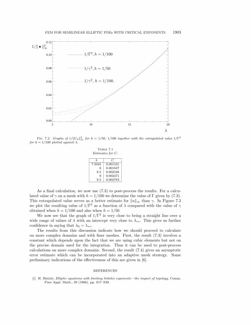
Fig. 7.2. Graphs of 1/‖Uh‖2∞ for h = 1/50, 1/100 together with the extrapolated value 1/Γ2
for h = 1/100 plotted against λ.
Table 7.1
Estimates for C.
λ C7.5045 0.001531
8 0.0018478.5 0.002168
9 0.0024719.5 0.002783
As a final calculation, we now use (7.3) to post-process the results. For a calcu-lated value of γ on a mesh with h = 1/100 we determine the value of Γ given by (7.3).This extrapolated value serves as a better estimate for ‖u‖∞ than γ. In Figure 7.2we plot the resulting value of 1/Γ2 as a function of λ compared with the value of γobtained when h = 1/100 and also when h = 1/50.
We now see that the graph of 1/Γ2 is very close to being a straight line over awide range of values of λ with an intercept very close to λ∗∗. This gives us furtherconfidence in saying that λ0 = λ∗∗.
The results from this discussion indicate how we should proceed to calculateon more complex domains and with finer meshes. First, the result (7.3) involves aconstant which depends upon the fact that we are using cubic elements but not onthe precise domain used for the integration. Thus it can be used to post-processcalculations on more complex domains. Second, the result (7.4) gives an asymptoticerror estimate which can be incorporated into an adaptive mesh strategy. Somepreliminary indications of the effectiveness of this are given in [6].
REFERENCES
[1] H. Brezis, Elliptic equations with limiting Sobolev exponents—the impact of topology, Comm.Pure Appl. Math., 39 (1986), pp. S17–S39.
1904 C. J. BUDD, A. R. HUMPHRIES, AND A. J. WATHEN
[2] H. Brezis and L. Nirenberg, Positive solutions of nonlinear elliptic equations involving crit-
ical Sobolev exponents, Comm. Pure Appl. Math., 36 (1983), pp. 437–477.[3] H. Brezis and L. Peletier, Asymptotics for elliptic equations involving critical growth, in
Partial Differential Equations and the Calculus of Variations, Volume I, Birkhauser, Boston,1989, pp. 149–192.
[4] C. Budd, Semilinear elliptic equations with near critical growth rates, Proc. Roy. Soc. Edin-burgh, Sect. A, 107 (1987), pp. 249–270.
[5] C. Budd and A. Humphries, Weak finite dimensional approximations of radial solutions of
semi-linear elliptic PDEs with near critical exponents, J. Asymptotic Anal., 17 (1998), pp.185–220.
[6] C. Budd and A. Humphries, Adaptive methods for semilinear elliptic equations with critical
exponents and interior singularities, Appl. Numer. Math., 26 (1998), pp. 227–240.[7] S. Chow and J. Hale, Methods of Bifurcation Theory, Springer-Verlag, New York, 1982.[8] M. Crouzeix and J. Rappaz, On Numerical Approximation in Bifurcation Theory, Springer-
Verlag, New York, 1989.[9] M. Dobrowolski and R. Rannacher, Finite element methods for nonlinear elliptic systems
of second order, Math. Nachr., 94 (1980), pp. 155–172.[10] W.-M. Gidas, B. Ni, and L. Nirenberg, Symmetry and related properties via the maximum
principle, Comm. Math. Phys., 68 (1979), pp. 209–243.[11] P. Lions, On the existence of positive solutions of semilinear elliptic equations, SIAM Rev.,
24 (1982), pp. 441–467.[12] J. Lopez-Marcos and J. Sanz-Serna, Stability and convergence in numerical analysis iii:
Linear investigation of nonlinear stability, IMA J. Numer. Anal., 8 (1986), pp. 71–84.[13] B. McLeod, A Nonlinear Elliptic Equation with Critical Sobolev Exponent, unpublished work,
1984.[14] F. Merle, L. Peletier, and J. Serrin, A bifurcation problem at a singular limit, Indiana
Univ. Math. J., 43 (1994), pp. 585–609.[15] T. Murdoch and C. Budd, Convergent and spurious solutions of nonlinear elliptic equations,
IMA J. Numer. Anal., 12 (1992), pp. 365–386.[16] R. Schoen, Conformal deformation of a Riemannian metric to constant scalar curvature,