239
The Fisher-KPP Equation and other Pulled Fronts Éric Brunet Laboratoire de Physique Statistique, É.N.S., UPMC, Paris Banff 2010 Éric Brunet (Paris) FKPP Equation Banff 2010 1 / 50

The Fisher-KPP Equation and other Pulled Fronts
Éric Brunet
Laboratoire de Physique Statistique, É.N.S., UPMC, Paris
Banff 2010
Éric Brunet (Paris) FKPP Equation Banff 2010 1 / 50
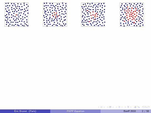
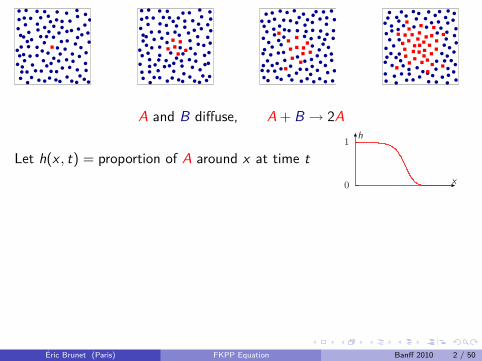
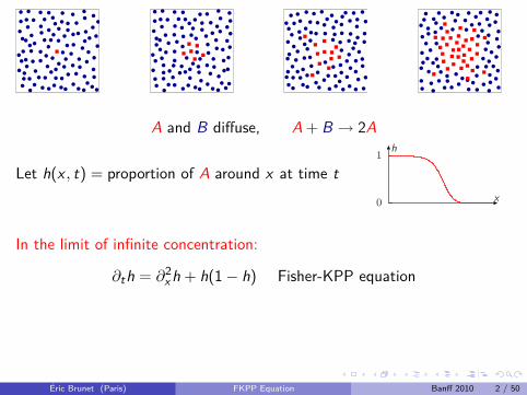
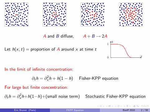
A and B diffuse, A + B → 2A
Let h(x , t) = proportion of A around x at time tx
h1
0
In the limit of infinite concentration:
∂th = ∂2x h + h(1− h) Fisher-KPP equation
For large but finite concentration:
∂th = ∂2x h+h(1−h)+(small noise term) Stochastic Fisher-KPP equation
Éric Brunet (Paris) FKPP Equation Banff 2010 2 / 50

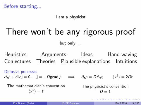
Before starting...
I am a physicist
There won’t be any rigorous proofbut only. . .
Heuristics Arguments Ideas Hand-wavingConjectures Theories Plausible explanations Intuitions
Diffusive processes∂tρ+ div j = 0, j = −Dgrad ρ =⇒ ∂tρ = D∆ρ; 〈x2〉 = 2Dt
The mathematician’s convention〈x2〉 = t
The physicist’s conventionD = 1
Éric Brunet (Paris) FKPP Equation Banff 2010 3 / 50

Before starting...
I am a physicist
There won’t be any rigorous proofbut only. . .
Heuristics Arguments Ideas Hand-wavingConjectures Theories Plausible explanations IntuitionsDiffusive processes∂tρ+ div j = 0, j = −Dgrad ρ =⇒ ∂tρ = D∆ρ; 〈x2〉 = 2Dt
The mathematician’s convention〈x2〉 = t
The physicist’s conventionD = 1
Éric Brunet (Paris) FKPP Equation Banff 2010 3 / 50

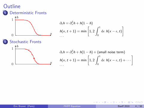
Outline1 Deterministic Fronts
x
h1
0
∂th = ∂2x h + h(1− h)
h(x , t + 1) = min[
1, 2∫ 1
0dε h(x − ε, t)
]. . .
2 Stochastic Fronts
x
h1
0
∂th = ∂2x h + h(1− h) + (small noise term)
h(x , t + 1) = min[
1, 2∫ 1
0dε h(x − ε, t) + · · ·
]. . .
3 Fronts and Branching Brownian Motion
Éric Brunet (Paris) FKPP Equation Banff 2010 4 / 50
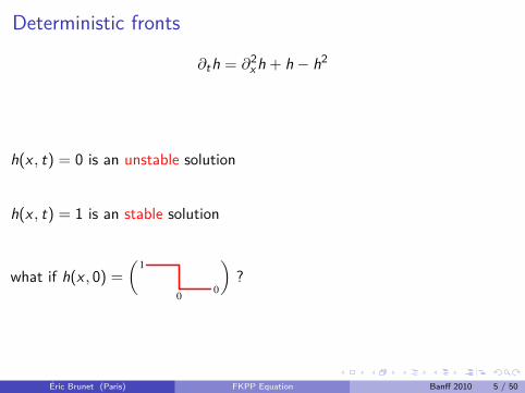
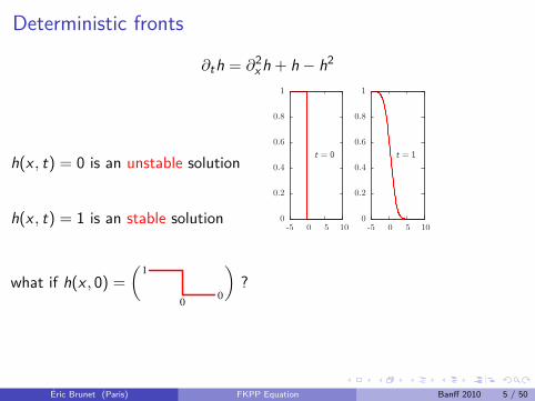
Deterministic fronts
∂th = ∂2x h + h − h2
h(x , t) = 0 is an unstable solution
h(x , t) = 1 is an stable solution
what if h(x , 0) =
(0
1
0
)?
t = 0
1050-5
1
0.8
0.6
0.4
0.2
0
t = 20t = 10t = 5
454035302520151050-5
1
0.8
0.6
0.4
0.2
0
Éric Brunet (Paris) FKPP Equation Banff 2010 5 / 50
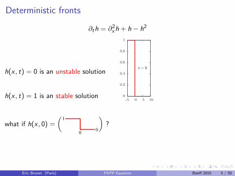
Deterministic fronts
∂th = ∂2x h + h − h2
h(x , t) = 0 is an unstable solution
h(x , t) = 1 is an stable solution
what if h(x , 0) =
(0
1
0
)?
t = 0
1050-5
1
0.8
0.6
0.4
0.2
0
t = 20t = 10t = 5
454035302520151050-5
1
0.8
0.6
0.4
0.2
0
Éric Brunet (Paris) FKPP Equation Banff 2010 5 / 50
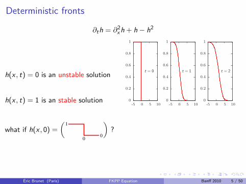
Deterministic fronts
∂th = ∂2x h + h − h2
h(x , t) = 0 is an unstable solution
h(x , t) = 1 is an stable solution
what if h(x , 0) =
(0
1
0
)?
t = 0
1050-5
1
0.8
0.6
0.4
0.2
0
t = 1
1050-5
1
0.8
0.6
0.4
0.2
0
t = 20t = 10t = 5
454035302520151050-5
1
0.8
0.6
0.4
0.2
0
Éric Brunet (Paris) FKPP Equation Banff 2010 5 / 50
Deterministic fronts
∂th = ∂2x h + h − h2
h(x , t) = 0 is an unstable solution
h(x , t) = 1 is an stable solution
what if h(x , 0) =
(0
1
0
)?
t = 0
1050-5
1
0.8
0.6
0.4
0.2
0
t = 1
1050-5
1
0.8
0.6
0.4
0.2
0
t = 2
1050-5
1
0.8
0.6
0.4
0.2
0
t = 20t = 10t = 5
454035302520151050-5
1
0.8
0.6
0.4
0.2
0
Éric Brunet (Paris) FKPP Equation Banff 2010 5 / 50

Deterministic fronts
∂th = ∂2x h + h − h2
h(x , t) = 0 is an unstable solution
h(x , t) = 1 is an stable solution
what if h(x , 0) =
(0
1
0
)?
t = 0
1050-5
1
0.8
0.6
0.4
0.2
0
t = 1
1050-5
1
0.8
0.6
0.4
0.2
0
t = 2
1050-5
1
0.8
0.6
0.4
0.2
0
t = 5
454035302520151050-5
1
0.8
0.6
0.4
0.2
0
t = 20t = 10t = 5
454035302520151050-5
1
0.8
0.6
0.4
0.2
0
Éric Brunet (Paris) FKPP Equation Banff 2010 5 / 50
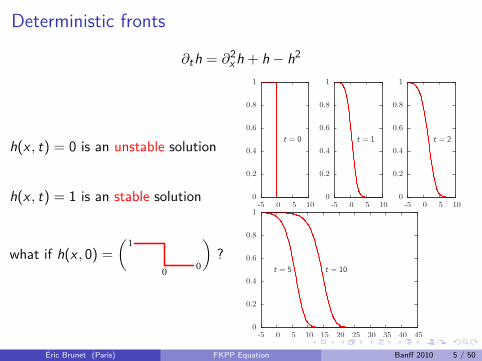
Deterministic fronts
∂th = ∂2x h + h − h2
h(x , t) = 0 is an unstable solution
h(x , t) = 1 is an stable solution
what if h(x , 0) =
(0
1
0
)?
t = 0
1050-5
1
0.8
0.6
0.4
0.2
0
t = 1
1050-5
1
0.8
0.6
0.4
0.2
0
t = 2
1050-5
1
0.8
0.6
0.4
0.2
0
t = 10t = 5
454035302520151050-5
1
0.8
0.6
0.4
0.2
0
t = 20t = 10t = 5
454035302520151050-5
1
0.8
0.6
0.4
0.2
0
Éric Brunet (Paris) FKPP Equation Banff 2010 5 / 50
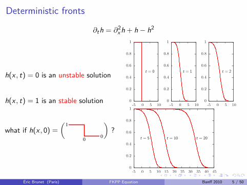
Deterministic fronts
∂th = ∂2x h + h − h2
h(x , t) = 0 is an unstable solution
h(x , t) = 1 is an stable solution
what if h(x , 0) =
(0
1
0
)?
t = 0
1050-5
1
0.8
0.6
0.4
0.2
0
t = 1
1050-5
1
0.8
0.6
0.4
0.2
0
t = 2
1050-5
1
0.8
0.6
0.4
0.2
0
t = 20t = 10t = 5
454035302520151050-5
1
0.8
0.6
0.4
0.2
0
Éric Brunet (Paris) FKPP Equation Banff 2010 5 / 50

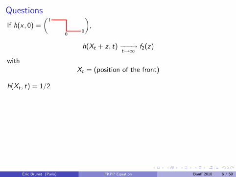
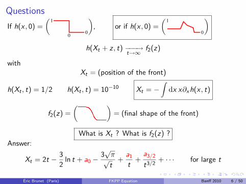
QuestionsIf h(x , 0) =
(0
1
0
),
or if h(x , 0) =
(0
1
0
)
h(Xt + z , t) −−−→t→∞
f2(z)
withXt = (position of the front)
h(Xt , t) = 1/2 h(Xt , t) = 10−10 Xt = −∫
dx x∂xh(x , t)
f2(z) =
( )= (final shape of the front)
What is Xt ? What is f2(z) ?Answer:
Xt = 2t − 32 ln t + a0 − 3√π√
t+
a1t +
a3/2t3/2 + · · · for large t
Éric Brunet (Paris) FKPP Equation Banff 2010 6 / 50
QuestionsIf h(x , 0) =
(0
1
0
),
or if h(x , 0) =
(0
1
0
)
h(Xt + z , t) −−−→t→∞
f2(z)
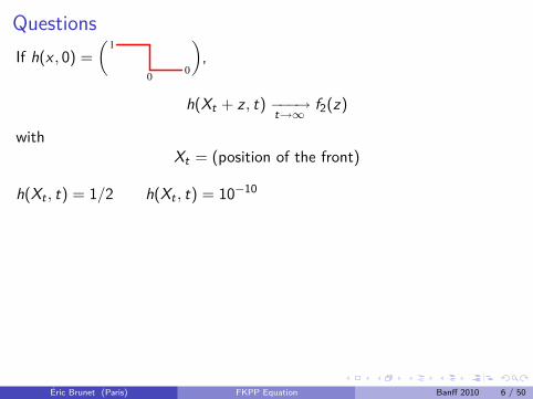
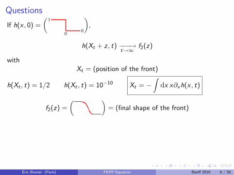
withXt = (position of the front)
h(Xt , t) = 1/2
h(Xt , t) = 10−10 Xt = −∫
dx x∂xh(x , t)
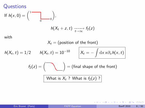
f2(z) =
( )= (final shape of the front)
What is Xt ? What is f2(z) ?Answer:
Xt = 2t − 32 ln t + a0 − 3√π√
t+
a1t +
a3/2t3/2 + · · · for large t
Éric Brunet (Paris) FKPP Equation Banff 2010 6 / 50
QuestionsIf h(x , 0) =
(0
1
0
),
or if h(x , 0) =
(0
1
0
)
h(Xt + z , t) −−−→t→∞
f2(z)
withXt = (position of the front)
h(Xt , t) = 1/2 h(Xt , t) = 10−10
Xt = −∫
dx x∂xh(x , t)
f2(z) =
( )= (final shape of the front)
What is Xt ? What is f2(z) ?Answer:
Xt = 2t − 32 ln t + a0 − 3√π√
t+
a1t +
a3/2t3/2 + · · · for large t
Éric Brunet (Paris) FKPP Equation Banff 2010 6 / 50

QuestionsIf h(x , 0) =
(0
1
0
),
or if h(x , 0) =
(0
1
0
)
h(Xt + z , t) −−−→t→∞
f2(z)
withXt = (position of the front)
h(Xt , t) = 1/2 h(Xt , t) = 10−10 Xt = −∫
dx x∂xh(x , t)
f2(z) =
( )= (final shape of the front)
What is Xt ? What is f2(z) ?Answer:
Xt = 2t − 32 ln t + a0 − 3√π√
t+
a1t +
a3/2t3/2 + · · · for large t
Éric Brunet (Paris) FKPP Equation Banff 2010 6 / 50
QuestionsIf h(x , 0) =
(0
1
0
),
or if h(x , 0) =
(0
1
0
)
h(Xt + z , t) −−−→t→∞
f2(z)
withXt = (position of the front)
h(Xt , t) = 1/2 h(Xt , t) = 10−10 Xt = −∫
dx x∂xh(x , t)
f2(z) =
( )= (final shape of the front)
What is Xt ? What is f2(z) ?
Answer:
Xt = 2t − 32 ln t + a0 − 3√π√
t+
a1t +
a3/2t3/2 + · · · for large t
Éric Brunet (Paris) FKPP Equation Banff 2010 6 / 50

QuestionsIf h(x , 0) =
(0
1
0
),
or if h(x , 0) =
(0
1
0
)
h(Xt + z , t) −−−→t→∞
f2(z)
withXt = (position of the front)
h(Xt , t) = 1/2 h(Xt , t) = 10−10 Xt = −∫
dx x∂xh(x , t)
f2(z) =
( )= (final shape of the front)
What is Xt ? What is f2(z) ?Answer:
Xt = 2t − 32 ln t + a0 − 3√π√
t+
a1t +
a3/2t3/2 + · · · for large t
Éric Brunet (Paris) FKPP Equation Banff 2010 6 / 50
QuestionsIf h(x , 0) =
(0
1
0
), or if h(x , 0) =
(0
1
0
)h(Xt + z , t) −−−→
t→∞f2(z)
withXt = (position of the front)
h(Xt , t) = 1/2 h(Xt , t) = 10−10 Xt = −∫
dx x∂xh(x , t)
f2(z) =
( )= (final shape of the front)
What is Xt ? What is f2(z) ?Answer:
Xt = 2t − 32 ln t + a0 − 3√π√
t+
a1t +
a3/2t3/2 + · · · for large t
Éric Brunet (Paris) FKPP Equation Banff 2010 6 / 50

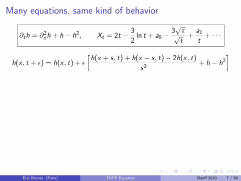
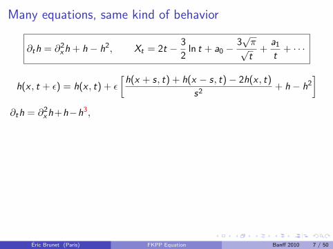
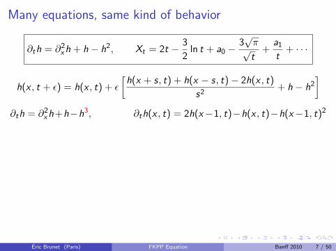
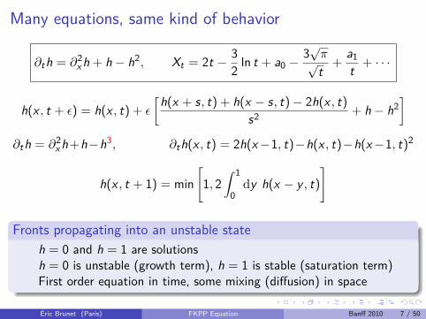
Many equations, same kind of behavior
∂th = ∂2x h + h − h2, Xt = 2t − 32 ln t + a0 − 3√π√
t+
a1t + · · ·
h(x , t + ε) = h(x , t) + ε
[h(x + s, t) + h(x − s, t)− 2h(x , t)
s2 + h − h2]
∂th = ∂2x h+h−h3, ∂th(x , t) = 2h(x−1, t)−h(x , t)−h(x−1, t)2
h(x , t + 1) = min[1, 2
∫ 1
0dy h(x − y , t)
]
Fronts propagating into an unstable stateh = 0 and h = 1 are solutionsh = 0 is unstable (growth term), h = 1 is stable (saturation term)First order equation in time, some mixing (diffusion) in space
Éric Brunet (Paris) FKPP Equation Banff 2010 7 / 50
Many equations, same kind of behavior
∂th = ∂2x h + h − h2, Xt = 2t − 32 ln t + a0 − 3√π√
t+
a1t + · · ·
h(x , t + ε) = h(x , t) + ε
[h(x + s, t) + h(x − s, t)− 2h(x , t)
s2 + h − h2]
∂th = ∂2x h+h−h3,
∂th(x , t) = 2h(x−1, t)−h(x , t)−h(x−1, t)2
h(x , t + 1) = min[1, 2
∫ 1
0dy h(x − y , t)
]
Fronts propagating into an unstable stateh = 0 and h = 1 are solutionsh = 0 is unstable (growth term), h = 1 is stable (saturation term)First order equation in time, some mixing (diffusion) in space
Éric Brunet (Paris) FKPP Equation Banff 2010 7 / 50
Many equations, same kind of behavior
∂th = ∂2x h + h − h2, Xt = 2t − 32 ln t + a0 − 3√π√
t+
a1t + · · ·
h(x , t + ε) = h(x , t) + ε
[h(x + s, t) + h(x − s, t)− 2h(x , t)
s2 + h − h2]
∂th = ∂2x h+h−h3, ∂th(x , t) = 2h(x−1, t)−h(x , t)−h(x−1, t)2
h(x , t + 1) = min[1, 2
∫ 1
0dy h(x − y , t)
]
Fronts propagating into an unstable stateh = 0 and h = 1 are solutionsh = 0 is unstable (growth term), h = 1 is stable (saturation term)First order equation in time, some mixing (diffusion) in space
Éric Brunet (Paris) FKPP Equation Banff 2010 7 / 50

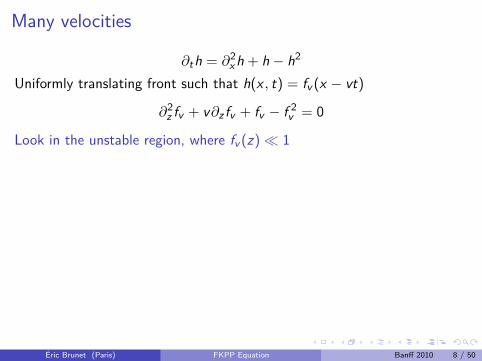
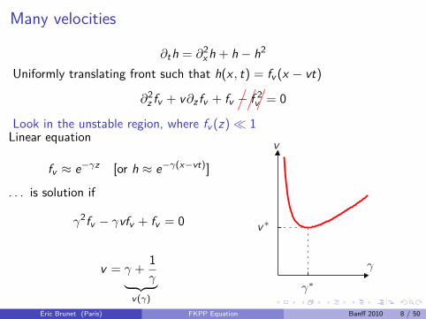
Many velocities
∂th = ∂2x h + h − h2
Uniformly translating front such that h(x , t) = fv (x − vt)
∂2z fv + v∂z fv + fv
///
− f 2v = 0
Look in the unstable region, where fv (z)� 1Linear equation
fv ≈ e−γz [or h ≈ e−γ(x−vt)]
. . . is solution if
γ2fv − γvfv + fv = 0
v = γ +1γ︸ ︷︷ ︸
v(γ)
γ
v
γ∗
v∗
Éric Brunet (Paris) FKPP Equation Banff 2010 8 / 50
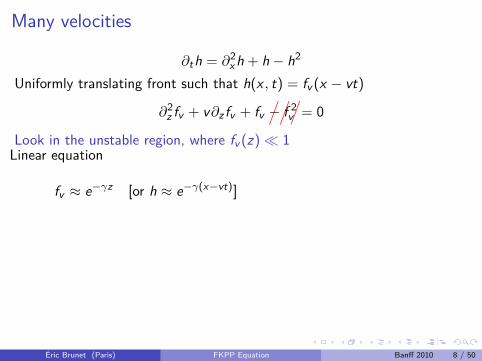
Many velocities
∂th = ∂2x h + h − h2
Uniformly translating front such that h(x , t) = fv (x − vt)
∂2z fv + v∂z fv + fv
///
− f 2v = 0
Look in the unstable region, where fv (z)� 1
Linear equation
fv ≈ e−γz [or h ≈ e−γ(x−vt)]
. . . is solution if
γ2fv − γvfv + fv = 0
v = γ +1γ︸ ︷︷ ︸
v(γ)
γ
v
γ∗
v∗
Éric Brunet (Paris) FKPP Equation Banff 2010 8 / 50

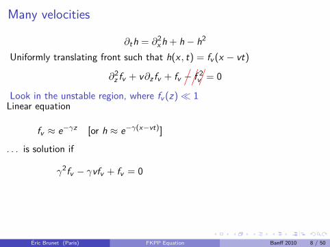
Many velocities
∂th = ∂2x h + h − h2
Uniformly translating front such that h(x , t) = fv (x − vt)
∂2z fv + v∂z fv + fv///− f 2v = 0
Look in the unstable region, where fv (z)� 1
Linear equation
fv ≈ e−γz [or h ≈ e−γ(x−vt)]
. . . is solution if
γ2fv − γvfv + fv = 0
v = γ +1γ︸ ︷︷ ︸
v(γ)
γ
v
γ∗
v∗
Éric Brunet (Paris) FKPP Equation Banff 2010 8 / 50
Many velocities
∂th = ∂2x h + h − h2
Uniformly translating front such that h(x , t) = fv (x − vt)
∂2z fv + v∂z fv + fv///− f 2v = 0
Look in the unstable region, where fv (z)� 1Linear equation
fv ≈ e−γz [or h ≈ e−γ(x−vt)]
. . . is solution if
γ2fv − γvfv + fv = 0
v = γ +1γ︸ ︷︷ ︸
v(γ)
γ
v
γ∗
v∗
Éric Brunet (Paris) FKPP Equation Banff 2010 8 / 50

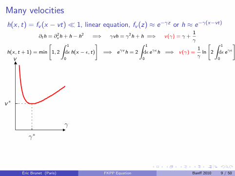
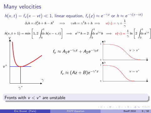
Many velocitiesh(x , t) = fv (x − vt)� 1, linear equation, fv (z) ≈ e−γz or h ≈ e−γ(x−vt)
∂th = ∂2x h + h − h2 =⇒ γvh = γ2h + h =⇒ v(γ) = γ +1γ
h(x , t + 1) = min[1, 2∫ 1
0dε h(x − ε, t)
]=⇒ eγv h = 2
∫ 1
0dε eγεh =⇒ v(γ) =
1γln[2∫ 1
0dε eγε
]
fv ≈ A1e−γ1z + A2e−γ2z v > v ∗
x
h1
0
fv ≈ (Az + B)e−γ∗z v = v ∗
x
h1
0
fv ≈ A sin(γIz + φ)e−γRz v < v ∗
x
h1
0
Fronts with v < v∗ are unstable
Éric Brunet (Paris) FKPP Equation Banff 2010 9 / 50
Many velocitiesh(x , t) = fv (x − vt)� 1, linear equation, fv (z) ≈ e−γz or h ≈ e−γ(x−vt)
∂th = ∂2x h + h − h2 =⇒ γvh = γ2h + h =⇒ v(γ) = γ +1γ
h(x , t + 1) = min[1, 2∫ 1
0dε h(x − ε, t)
]=⇒ eγv h = 2
∫ 1
0dε eγεh =⇒ v(γ) =
1γln[2∫ 1
0dε eγε
]
γ
v
γ∗
v∗
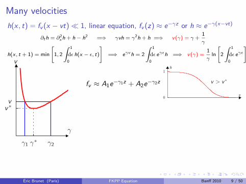
fv ≈ A1e−γ1z + A2e−γ2z v > v ∗
x
h1
0
fv ≈ (Az + B)e−γ∗z v = v ∗
x
h1
0
fv ≈ A sin(γIz + φ)e−γRz v < v ∗
x
h1
0
Fronts with v < v∗ are unstable
Éric Brunet (Paris) FKPP Equation Banff 2010 9 / 50
Many velocitiesh(x , t) = fv (x − vt)� 1, linear equation, fv (z) ≈ e−γz or h ≈ e−γ(x−vt)
∂th = ∂2x h + h − h2 =⇒ γvh = γ2h + h =⇒ v(γ) = γ +1γ
h(x , t + 1) = min[1, 2∫ 1
0dε h(x − ε, t)
]=⇒ eγv h = 2
∫ 1
0dε eγεh =⇒ v(γ) =
1γln[2∫ 1
0dε eγε
]
γ
v
γ2γ∗γ1
vv∗
fv ≈ A1e−γ1z + A2e−γ2z v > v ∗
x
h1
0
fv ≈ (Az + B)e−γ∗z v = v ∗
x
h1
0
fv ≈ A sin(γIz + φ)e−γRz v < v ∗
x
h1
0
Fronts with v < v∗ are unstable
Éric Brunet (Paris) FKPP Equation Banff 2010 9 / 50
Many velocitiesh(x , t) = fv (x − vt)� 1, linear equation, fv (z) ≈ e−γz or h ≈ e−γ(x−vt)
∂th = ∂2x h + h − h2 =⇒ γvh = γ2h + h =⇒ v(γ) = γ +1γ
h(x , t + 1) = min[1, 2∫ 1
0dε h(x − ε, t)
]=⇒ eγv h = 2
∫ 1
0dε eγεh =⇒ v(γ) =
1γln[2∫ 1
0dε eγε
]
γ
v
γ∗
v∗
fv ≈ A1e−γ1z + A2e−γ2z v > v ∗
x
h1
0
fv ≈ (Az + B)e−γ∗z v = v ∗
x
h1
0
fv ≈ A sin(γIz + φ)e−γRz v < v ∗
x
h1
0
Fronts with v < v∗ are unstable
Éric Brunet (Paris) FKPP Equation Banff 2010 9 / 50

Many velocitiesh(x , t) = fv (x − vt)� 1, linear equation, fv (z) ≈ e−γz or h ≈ e−γ(x−vt)
∂th = ∂2x h + h − h2 =⇒ γvh = γ2h + h =⇒ v(γ) = γ +1γ
h(x , t + 1) = min[1, 2∫ 1
0dε h(x − ε, t)
]=⇒ eγv h = 2
∫ 1
0dε eγεh =⇒ v(γ) =
1γln[2∫ 1
0dε eγε
]
γ
v
γ∗
v∗v
fv ≈ A1e−γ1z + A2e−γ2z v > v ∗
x
h1
0
fv ≈ (Az + B)e−γ∗z v = v ∗
x
h1
0
fv ≈ A sin(γIz + φ)e−γRz v < v ∗
x
h1
0
Fronts with v < v∗ are unstable
Éric Brunet (Paris) FKPP Equation Banff 2010 9 / 50
Many velocitiesh(x , t) = fv (x − vt)� 1, linear equation, fv (z) ≈ e−γz or h ≈ e−γ(x−vt)
∂th = ∂2x h + h − h2 =⇒ γvh = γ2h + h =⇒ v(γ) = γ +1γ
h(x , t + 1) = min[1, 2∫ 1
0dε h(x − ε, t)
]=⇒ eγv h = 2
∫ 1
0dε eγεh =⇒ v(γ) =
1γln[2∫ 1
0dε eγε
]
γ
v
γ∗
v∗
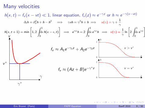
fv ≈ A1e−γ1z + A2e−γ2z v > v ∗
x
h1
0
fv ≈ (Az + B)e−γ∗z v = v ∗
x
h1
0
fv ≈ A sin(γIz + φ)e−γRz v < v ∗
x
h1
0
Fronts with v < v∗ are unstable
Éric Brunet (Paris) FKPP Equation Banff 2010 9 / 50
Linear perturbation
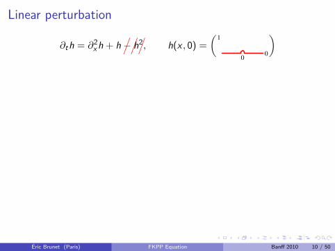
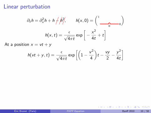
∂th = ∂2x h + h///− h2, h(x , 0) =
(1
00
)
h(x , t) =ε√4πt
exp[− x2
4t + t]
At a position x = vt + y
h(vt + y , t) =ε√4πt
exp[(
1− v2
4
)t − vy
2 −y2
4t
]
A linear perturbation movesat velocity v = v∗ (= 2)
h(2t + y , t) =ε√4πt
exp[− y − y2
4t
]At a position x = 2t − 1
2 ln t + z
h(2t − 12 ln t + z) = ε
1√4π
//
texp
[− z +
///
12 ln t − z2
4t + · · ·]
Éric Brunet (Paris) FKPP Equation Banff 2010 10 / 50

Linear perturbation
∂th = ∂2x h + h///− h2, h(x , 0) =
(1
00
)
h(x , t) =ε√4πt
exp[− x2
4t + t]
At a position x = vt + y
h(vt + y , t) =ε√4πt
exp[(
1− v2
4
)t − vy
2 −y2
4t
]
A linear perturbation movesat velocity v = v∗ (= 2)
h(2t + y , t) =ε√4πt
exp[− y − y2
4t
]At a position x = 2t − 1
2 ln t + z
h(2t − 12 ln t + z) = ε
1√4π
//
texp
[− z +
///
12 ln t − z2
4t + · · ·]
Éric Brunet (Paris) FKPP Equation Banff 2010 10 / 50

Linear perturbation
∂th = ∂2x h + h///− h2, h(x , 0) =
(1
00
)
h(x , t) =ε√4πt
exp[− x2
4t + t]
At a position x = vt + y
h(vt + y , t) =ε√4πt
exp[(
1− v2
4
)t − vy
2 −y2
4t
]
A linear perturbation movesat velocity v = v∗ (= 2)
h(2t + y , t) =ε√4πt
exp[− y − y2
4t
]
At a position x = 2t − 12 ln t + z
h(2t − 12 ln t + z) = ε
1√4π
//
texp
[− z +
///
12 ln t − z2
4t + · · ·]
Éric Brunet (Paris) FKPP Equation Banff 2010 10 / 50

Linear perturbation
∂th = ∂2x h + h///− h2, h(x , 0) =
(1
00
)
h(x , t) =ε√4πt
exp[− x2
4t + t]
At a position x = vt + y
h(vt + y , t) =ε√4πt
exp[(
1− v2
4
)t − vy
2 −y2
4t
]
A linear perturbation movesat velocity v = v∗ (= 2)
h(2t + y , t) =ε√4πt
exp[− y − y2
4t
]At a position x = 2t − 1
2 ln t + z
h(2t − 12 ln t + z) = ε
1√4π
//
texp
[− z +
///
12 ln t − z2
4t + · · ·]
Éric Brunet (Paris) FKPP Equation Banff 2010 10 / 50

Linear perturbation
∂th = ∂2x h + h///− h2, h(x , 0) =
(1
00
)
h(x , t) =ε√4πt
exp[− x2
4t + t]
At a position x = vt + y
h(vt + y , t) =ε√4πt
exp[(
1− v2
4
)t − vy
2 −y2
4t
]
A linear perturbation movesat velocity v = v∗ (= 2)
h(2t + y , t) =ε√4πt
exp[− y − y2
4t
]At a position x = 2t − 1
2 ln t + z
h(2t − 12 ln t + z) = ε
1√4π//t
exp[− z +
///12 ln t − z2
4t + · · ·]
Éric Brunet (Paris) FKPP Equation Banff 2010 10 / 50

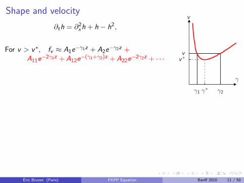
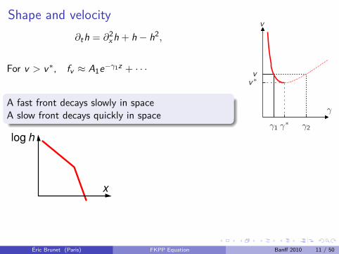
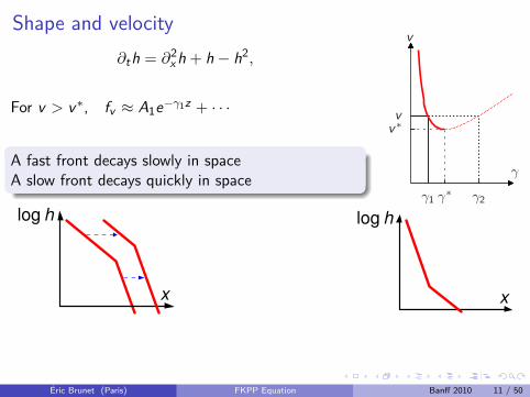
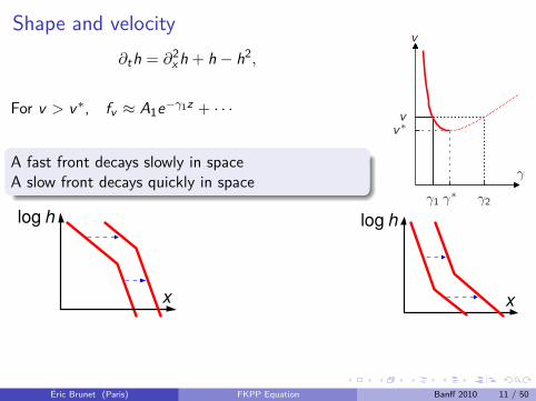
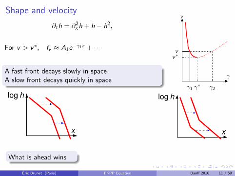
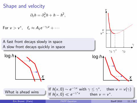
Shape and velocity∂th = ∂2x h + h
///− h2,
For v > v∗, fv ≈ A1e−γ1z + A2e−γ2z
+A11e−2γ1z + A12e−(γ1+γ2)z + A22e−2γ2z + · · ·
A fast front decays slowly in spaceA slow front decays quickly in space
γ
v
γ2γ∗γ1
vv∗
What is ahead wins If h(x , 0) ∼ e−γx with γ ≤ γ∗, then v = v(γ)If h(x , 0)� e−γ∗x then v = v∗.
Éric Brunet (Paris) FKPP Equation Banff 2010 11 / 50
Shape and velocity∂th = ∂2x h + h
///
− h2,
For v > v∗, fv ≈ A1e−γ1z + A2e−γ2z +A11e−2γ1z + A12e−(γ1+γ2)z + A22e−2γ2z + · · ·
A fast front decays slowly in spaceA slow front decays quickly in space
γ
v
γ2γ∗γ1
vv∗
What is ahead wins If h(x , 0) ∼ e−γx with γ ≤ γ∗, then v = v(γ)If h(x , 0)� e−γ∗x then v = v∗.
Éric Brunet (Paris) FKPP Equation Banff 2010 11 / 50

Shape and velocity∂th = ∂2x h + h
///
− h2,
For v > v∗, fv ≈ A1e−γ1z + · · ·
+ A2e−γ2z +A11e−2γ1z + A12e−(γ1+γ2)z + A22e−2γ2z + · · ·
A fast front decays slowly in spaceA slow front decays quickly in space γ
v
γ2γ∗γ1
vv∗
What is ahead wins If h(x , 0) ∼ e−γx with γ ≤ γ∗, then v = v(γ)If h(x , 0)� e−γ∗x then v = v∗.
Éric Brunet (Paris) FKPP Equation Banff 2010 11 / 50
Shape and velocity∂th = ∂2x h + h
///
− h2,
For v > v∗, fv ≈ A1e−γ1z + · · ·
+ A2e−γ2z +A11e−2γ1z + A12e−(γ1+γ2)z + A22e−2γ2z + · · ·
A fast front decays slowly in spaceA slow front decays quickly in space γ
v
γ2γ∗γ1
vv∗
hlog
x
What is ahead wins If h(x , 0) ∼ e−γx with γ ≤ γ∗, then v = v(γ)If h(x , 0)� e−γ∗x then v = v∗.
Éric Brunet (Paris) FKPP Equation Banff 2010 11 / 50
Shape and velocity∂th = ∂2x h + h
///
− h2,
For v > v∗, fv ≈ A1e−γ1z + · · ·
+ A2e−γ2z +A11e−2γ1z + A12e−(γ1+γ2)z + A22e−2γ2z + · · ·
A fast front decays slowly in spaceA slow front decays quickly in space γ
v
γ2γ∗γ1
vv∗
hlog
x
hlog
x
What is ahead wins
If h(x , 0) ∼ e−γx with γ ≤ γ∗, then v = v(γ)If h(x , 0)� e−γ∗x then v = v∗.
Éric Brunet (Paris) FKPP Equation Banff 2010 11 / 50
Shape and velocity∂th = ∂2x h + h
///
− h2,
For v > v∗, fv ≈ A1e−γ1z + · · ·
+ A2e−γ2z +A11e−2γ1z + A12e−(γ1+γ2)z + A22e−2γ2z + · · ·
A fast front decays slowly in spaceA slow front decays quickly in space γ
v
γ2γ∗γ1
vv∗
hlog
x
hlog
x
What is ahead wins If h(x , 0) ∼ e−γx with γ ≤ γ∗, then v = v(γ)If h(x , 0)� e−γ∗x then v = v∗.
Éric Brunet (Paris) FKPP Equation Banff 2010 11 / 50

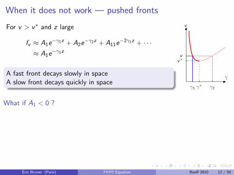
When it does not work — pushed frontsFor v > v∗ and z large
fv ≈ A1e−γ1z + A2e−γ2z + A11e−2γ1z + · · ·≈ A1e−γ1z
A fast front decays slowly in spaceA slow front decays quickly in space
γ
v
γ2γ∗γ1
vv∗
What if A1 < 0 ?
x
h1
0
A1 depends on v
A1 > 0
A1 < 0
γ
v
γc2γ∗γc
1
v c
v∗v = v(γ) if
{h(x , 0) ∼ e−γx
with γ ≤ γc1
v = v c if h(x , 0)� e−γc1x
Éric Brunet (Paris) FKPP Equation Banff 2010 12 / 50
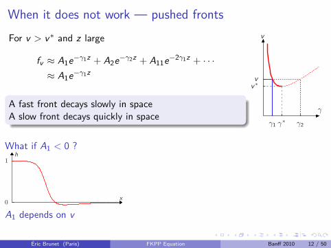

When it does not work — pushed frontsFor v > v∗ and z large
fv ≈ A1e−γ1z + A2e−γ2z + A11e−2γ1z + · · ·≈ A1e−γ1z
A fast front decays slowly in spaceA slow front decays quickly in space
γ
v
γ2γ∗γ1
vv∗
What if A1 < 0 ?
x
h1
0
A1 depends on v
A1 > 0
A1 < 0
γ
v
γc2γ∗γc
1
v c
v∗
v = v(γ) if{
h(x , 0) ∼ e−γx
with γ ≤ γc1
v = v c if h(x , 0)� e−γc1x
Éric Brunet (Paris) FKPP Equation Banff 2010 12 / 50

When it does not work — pushed frontsFor v > v∗ and z large
fv ≈ A1e−γ1z + A2e−γ2z + A11e−2γ1z + · · ·≈ A1e−γ1z
A fast front decays slowly in spaceA slow front decays quickly in space
γ
v
γ2γ∗γ1
vv∗
What if A1 < 0 ?
x
h1
0
A1 depends on v
A1 > 0
A1 < 0
γ
v
γc2γ∗γc
1
v c
v∗v = v(γ) if
{h(x , 0) ∼ e−γx
with γ ≤ γc1
v = v c if h(x , 0)� e−γc1x
Éric Brunet (Paris) FKPP Equation Banff 2010 12 / 50

SummaryPulled fronts propagating into an unstable state
x
h1
0
v < v∗, unstable
x
h1
0
v ≥ v∗, stable
Pushed fronts propagating into an unstable state
x
h1
0
v < v∗, unstablex
h1
0
v∗ ≤ v < v c , unstablex
h1
0
v ≥ v c , stable
An initial condition decaying fast enough leads to the slowest stable frontA pulled front goes at the same speed as a linear perturbationA pushed front goes faster than a linear perturbationA front can be pushed only if the non-linearities increase the growth rate
Éric Brunet (Paris) FKPP Equation Banff 2010 13 / 50

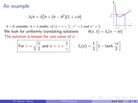
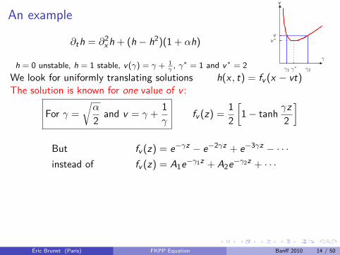
An example
∂th = ∂2x h + (h − h2)(1 + αh)
h = 0 unstable, h = 1 stable, v(γ) = γ + 1γ
, γ∗ = 1 and v∗ = 2γ
v
γ2γ∗γ1
vv∗
We look for uniformly translating solutions h(x , t) = fv (x − vt)The solution is known for one value of v :
For γ =
√α
2 and v = γ +1γ
fv (z) =12
[1− tanh γz
2
]
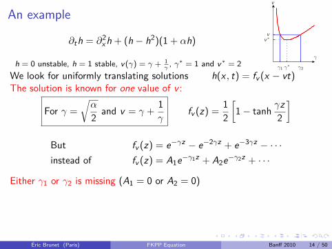
But fv (z) = e−γz − e−2γz + e−3γz − · · ·instead of fv (z) = A1e−γ1z + A2e−γ2z + · · ·
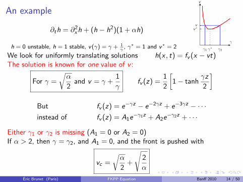
Either γ1 or γ2 is missing (A1 = 0 or A2 = 0)If α > 2, then γ = γ2, and A1 = 0, and the front is pushed with
vc =
√α
2 +
√2α
Éric Brunet (Paris) FKPP Equation Banff 2010 14 / 50

An example
∂th = ∂2x h + (h − h2)(1 + αh)
h = 0 unstable, h = 1 stable, v(γ) = γ + 1γ
, γ∗ = 1 and v∗ = 2γ
v
γ2γ∗γ1
vv∗
We look for uniformly translating solutions h(x , t) = fv (x − vt)The solution is known for one value of v :
For γ =
√α
2 and v = γ +1γ
fv (z) =12
[1− tanh γz
2
]
But fv (z) = e−γz − e−2γz + e−3γz − · · ·instead of fv (z) = A1e−γ1z + A2e−γ2z + · · ·
Either γ1 or γ2 is missing (A1 = 0 or A2 = 0)If α > 2, then γ = γ2, and A1 = 0, and the front is pushed with
vc =
√α
2 +
√2α
Éric Brunet (Paris) FKPP Equation Banff 2010 14 / 50
An example
∂th = ∂2x h + (h − h2)(1 + αh)
h = 0 unstable, h = 1 stable, v(γ) = γ + 1γ
, γ∗ = 1 and v∗ = 2γ
v
γ2γ∗γ1
vv∗
We look for uniformly translating solutions h(x , t) = fv (x − vt)The solution is known for one value of v :
For γ =
√α
2 and v = γ +1γ
fv (z) =12
[1− tanh γz
2
]
But fv (z) = e−γz − e−2γz + e−3γz − · · ·instead of fv (z) = A1e−γ1z + A2e−γ2z + · · ·
Either γ1 or γ2 is missing (A1 = 0 or A2 = 0)
If α > 2, then γ = γ2, and A1 = 0, and the front is pushed with
vc =
√α
2 +
√2α
Éric Brunet (Paris) FKPP Equation Banff 2010 14 / 50
An example
∂th = ∂2x h + (h − h2)(1 + αh)
h = 0 unstable, h = 1 stable, v(γ) = γ + 1γ
, γ∗ = 1 and v∗ = 2γ
v
γ2γ∗γ1
vv∗
We look for uniformly translating solutions h(x , t) = fv (x − vt)The solution is known for one value of v :
For γ =
√α
2 and v = γ +1γ
fv (z) =12
[1− tanh γz
2
]
But fv (z) = e−γz − e−2γz + e−3γz − · · ·instead of fv (z) = A1e−γ1z + A2e−γ2z + · · ·
Either γ1 or γ2 is missing (A1 = 0 or A2 = 0)If α > 2, then γ = γ2, and A1 = 0, and the front is pushed with
vc =
√α
2 +
√2α
Éric Brunet (Paris) FKPP Equation Banff 2010 14 / 50
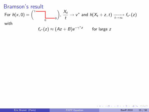
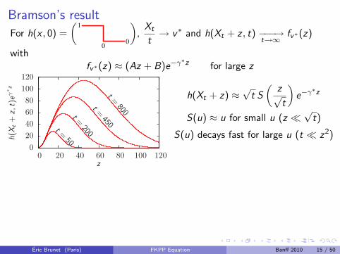
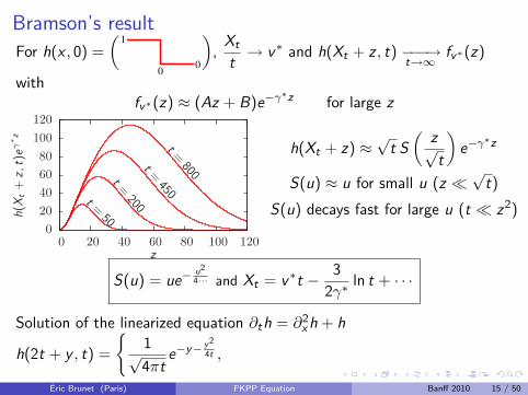
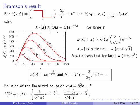
Bramson’s resultFor h(x , 0) =
(0
1
0
), Xt
t → v∗ and h(Xt + z , t) −−−→t→∞
fv∗(z)
withfv∗(z) ≈ (Az + B)e−γ∗z for large z
t =800t =
450
t =200t =
50
z
h(X t
+z,
t)eγ∗ z
120100806040200
120100806040200
h(Xt + z) ≈ √t S( z√
t
)e−γ∗z
S(u) ≈ u for small u (z � √t)S(u) decays fast for large u (t � z2)
S(u) = ue− u24··· and Xt = v∗t − 3
2γ∗ ln t + · · ·
Solution of the linearized equation ∂th = ∂2x h + h
h(2t + y , t) =
{1√4πt
e−y− y24t ,
1 + y2t√
4πte−y− y2
4t ,y√
4πt3/2e−y− y2
4t
}
Éric Brunet (Paris) FKPP Equation Banff 2010 15 / 50
Bramson’s resultFor h(x , 0) =
(0
1
0
), Xt
t → v∗ and h(Xt + z , t) −−−→t→∞
fv∗(z)
withfv∗(z) ≈ (Az + B)e−γ∗z for large z
t =800t =
450
t =200t =
50
z
h(X t
+z,
t)eγ∗ z
120100806040200
120100806040200
h(Xt + z) ≈ √t S( z√
t
)e−γ∗z
S(u) ≈ u for small u (z � √t)S(u) decays fast for large u (t � z2)
S(u) = ue− u24··· and Xt = v∗t − 3
2γ∗ ln t + · · ·
Solution of the linearized equation ∂th = ∂2x h + h
h(2t + y , t) =
{1√4πt
e−y− y24t ,
1 + y2t√
4πte−y− y2
4t ,
y√4πt3/2
e−y− y24t
}
Éric Brunet (Paris) FKPP Equation Banff 2010 15 / 50

Bramson’s resultFor h(x , 0) =
(0
1
0
), Xt
t → v∗ and h(Xt + z , t) −−−→t→∞
fv∗(z)
withfv∗(z) ≈ (Az + B)e−γ∗z for large z
t =800t =
450
t =200t =
50
z
h(X t
+z,
t)eγ∗ z
120100806040200
120100806040200
h(Xt + z) ≈ √t S( z√
t
)e−γ∗z
S(u) ≈ u for small u (z � √t)S(u) decays fast for large u (t � z2)
S(u) = ue− u24··· and Xt = v∗t − 3
2γ∗ ln t + · · ·
Solution of the linearized equation ∂th = ∂2x h + h
h(2t + y , t) =
{1√4πt
e−y− y24t ,
1 + y2t√
4πte−y− y2
4t ,y√
4πt3/2e−y− y2
4t
}Éric Brunet (Paris) FKPP Equation Banff 2010 15 / 50
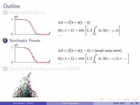
Outline1 Deterministic Fronts
x
h1
0
∂th = ∂2x h + h(1− h)
h(x , t + 1) = min[
1, 2∫ 1
0dε h(x − ε, t)
]. . .
2 Stochastic Fronts
x
h1
0
∂th = ∂2x h + h(1− h) + (small noise term)
h(x , t + 1) = min[
1, 2∫ 1
0dε h(x − ε, t) + · · ·
]. . .
3 Fronts and Branching Brownian Motion
Éric Brunet (Paris) FKPP Equation Banff 2010 16 / 50

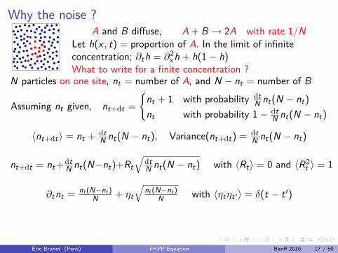
Why the noise ?A and B diffuse, A + B → 2A
with rate 1/N
Let h(x , t) = proportion of A. In the limit of infiniteconcentration; ∂th = ∂2x h + h(1− h)What to write for a finite concentration ?
N particles on one site, nt = number of A, and N − nt = number of B
Assuming nt given, nt+dt =
{nt + 1 with probability dt
N nt(N − nt)
nt with probability 1− dtN nt(N − nt)
〈nt+dt〉 = nt + dtN nt(N − nt), Variance(nt+dt) = dt
N nt(N − nt)
nt+dt = nt+dtN nt(N−nt)+Rt
√dtN nt(N − nt) with 〈Rt〉 = 0 and 〈R2
t 〉 = 1
∂tnt = nt (N−nt )N + ηt
√nt (N−nt )
N with 〈ηtηt′〉 = δ(t − t ′)
With h =ntN , ∂th =
∂2x h +
h(1− h) + ηt
√h(1− h)
N
Éric Brunet (Paris) FKPP Equation Banff 2010 17 / 50
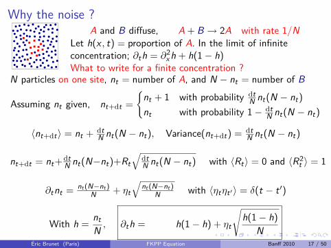
Why the noise ?A and B diffuse, A + B → 2A with rate 1/N
Let h(x , t) = proportion of A. In the limit of infiniteconcentration; ∂th = ∂2x h + h(1− h)What to write for a finite concentration ?
N particles on one site, nt = number of A, and N − nt = number of B
Assuming nt given, nt+dt =
{nt + 1 with probability dt
N nt(N − nt)
nt with probability 1− dtN nt(N − nt)
〈nt+dt〉 = nt + dtN nt(N − nt), Variance(nt+dt) = dt
N nt(N − nt)
nt+dt = nt+dtN nt(N−nt)+Rt
√dtN nt(N − nt) with 〈Rt〉 = 0 and 〈R2
t 〉 = 1
∂tnt = nt (N−nt )N + ηt
√nt (N−nt )
N with 〈ηtηt′〉 = δ(t − t ′)
With h =ntN , ∂th =
∂2x h +
h(1− h) + ηt
√h(1− h)
N
Éric Brunet (Paris) FKPP Equation Banff 2010 17 / 50
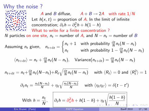
Why the noise ?A and B diffuse, A + B → 2A with rate 1/N
Let h(x , t) = proportion of A. In the limit of infiniteconcentration; ∂th = ∂2x h + h(1− h)What to write for a finite concentration ?
N particles on one site, nt = number of A, and N − nt = number of B
Assuming nt given, nt+dt =
{nt + 1 with probability dt
N nt(N − nt)
nt with probability 1− dtN nt(N − nt)
〈nt+dt〉 = nt + dtN nt(N − nt), Variance(nt+dt) = dt
N nt(N − nt)
nt+dt = nt+dtN nt(N−nt)+Rt
√dtN nt(N − nt) with 〈Rt〉 = 0 and 〈R2
t 〉 = 1
∂tnt = nt (N−nt )N + ηt
√nt (N−nt )
N with 〈ηtηt′〉 = δ(t − t ′)
With h =ntN , ∂th =
∂2x h +
h(1− h) + ηt
√h(1− h)
NÉric Brunet (Paris) FKPP Equation Banff 2010 17 / 50
Why the noise ?A and B diffuse, A + B → 2A with rate 1/N
Let h(x , t) = proportion of A. In the limit of infiniteconcentration; ∂th = ∂2x h + h(1− h)What to write for a finite concentration ?
N particles on one site, nt = number of A, and N − nt = number of B
Assuming nt given, nt+dt =
{nt + 1 with probability dt
N nt(N − nt)
nt with probability 1− dtN nt(N − nt)
〈nt+dt〉 = nt + dtN nt(N − nt), Variance(nt+dt) = dt
N nt(N − nt)
nt+dt = nt+dtN nt(N−nt)+Rt
√dtN nt(N − nt) with 〈Rt〉 = 0 and 〈R2
t 〉 = 1
∂tnt = nt (N−nt )N + ηt
√nt (N−nt )
N with 〈ηtηt′〉 = δ(t − t ′)
With h =ntN , ∂th = ∂2x h + h(1− h) + ηt
√h(1− h)
NÉric Brunet (Paris) FKPP Equation Banff 2010 17 / 50

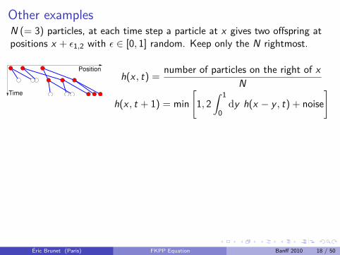
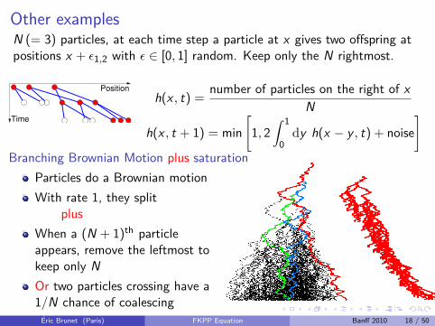
Other examplesN (= 3) particles, at each time step a particle at x gives two offspring atpositions x + ε1,2 with ε ∈ [0, 1] random. Keep only the N rightmost.
Position
Time
h(x , t) =number of particles on the right of x
N
h(x , t + 1) = min[1, 2
∫ 1
0dy h(x − y , t) + noise
]Branching Brownian Motion plus saturation
Particles do a Brownian motionWith rate 1, they split
plus
When a (N + 1)th particleappears, remove the leftmost tokeep only NOr two particles crossing have a1/N chance of coalescing
Éric Brunet (Paris) FKPP Equation Banff 2010 18 / 50
Other examplesN (= 3) particles, at each time step a particle at x gives two offspring atpositions x + ε1,2 with ε ∈ [0, 1] random. Keep only the N rightmost.
Position
Time
h(x , t) =number of particles on the right of x
N
h(x , t + 1) = min[1, 2
∫ 1
0dy h(x − y , t) + noise
]
Branching Brownian Motion plus saturationParticles do a Brownian motionWith rate 1, they split
plus
When a (N + 1)th particleappears, remove the leftmost tokeep only NOr two particles crossing have a1/N chance of coalescing
Éric Brunet (Paris) FKPP Equation Banff 2010 18 / 50

Other examplesN (= 3) particles, at each time step a particle at x gives two offspring atpositions x + ε1,2 with ε ∈ [0, 1] random. Keep only the N rightmost.
Position
Time
h(x , t) =number of particles on the right of x
N
h(x , t + 1) = min[1, 2
∫ 1
0dy h(x − y , t) + noise
]Branching Brownian Motion plus saturation
Particles do a Brownian motionWith rate 1, they split
plus
When a (N + 1)th particleappears, remove the leftmost tokeep only NOr two particles crossing have a1/N chance of coalescing
Éric Brunet (Paris) FKPP Equation Banff 2010 18 / 50

Other examplesN (= 3) particles, at each time step a particle at x gives two offspring atpositions x + ε1,2 with ε ∈ [0, 1] random. Keep only the N rightmost.
Position
Time
h(x , t) =number of particles on the right of x
N
h(x , t + 1) = min[1, 2
∫ 1
0dy h(x − y , t) + noise
]Branching Brownian Motion plus saturation
Particles do a Brownian motionWith rate 1, they split
plusWhen a (N + 1)th particleappears, remove the leftmost tokeep only N
Or two particles crossing have a1/N chance of coalescing
Éric Brunet (Paris) FKPP Equation Banff 2010 18 / 50
Other examplesN (= 3) particles, at each time step a particle at x gives two offspring atpositions x + ε1,2 with ε ∈ [0, 1] random. Keep only the N rightmost.
Position
Time
h(x , t) =number of particles on the right of x
N
h(x , t + 1) = min[1, 2
∫ 1
0dy h(x − y , t) + noise
]Branching Brownian Motion plus saturation
Particles do a Brownian motionWith rate 1, they split
plusWhen a (N + 1)th particleappears, remove the leftmost tokeep only NOr two particles crossing have a1/N chance of coalescingÉric Brunet (Paris) FKPP Equation Banff 2010 18 / 50
The noise term
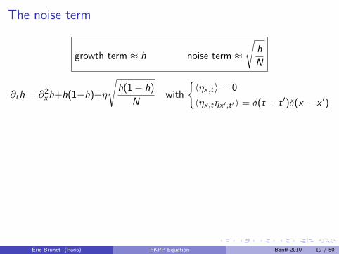
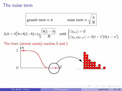
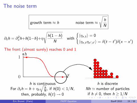
growth term ≈ h noise term ≈√
hN
∂th = ∂2x h+h(1−h)+η
√h(1− h)
N with{〈ηx ,t〉 = 0〈ηx ,tηx ′,t′〉 = δ(t − t ′)δ(x − x ′)
The front (almost surely) reaches 0 and 1
x
h1
0h is continuous
For ∂th = h + ηt√
hN , if h(0) < 1/N,
then, probably, h(t)→ 0
h is discreteNh ' number of particlesif h 6= 0, then h ≥ 1/N
Éric Brunet (Paris) FKPP Equation Banff 2010 19 / 50

The noise term
growth term ≈ h noise term ≈√
hN
∂th = ∂2x h+h(1−h)+η
√h(1− h)
N with{〈ηx ,t〉 = 0〈ηx ,tηx ′,t′〉 = δ(t − t ′)δ(x − x ′)
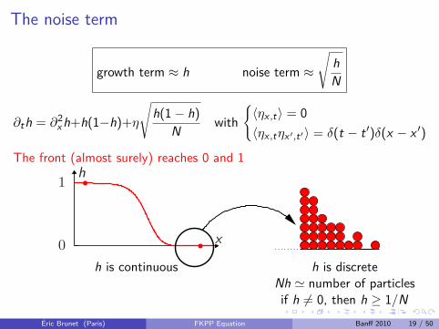
The front (almost surely) reaches 0 and 1
x
h1
0
h is continuous
For ∂th = h + ηt√
hN , if h(0) < 1/N,
then, probably, h(t)→ 0
h is discreteNh ' number of particlesif h 6= 0, then h ≥ 1/N
Éric Brunet (Paris) FKPP Equation Banff 2010 19 / 50
The noise term
growth term ≈ h noise term ≈√
hN
∂th = ∂2x h+h(1−h)+η
√h(1− h)
N with{〈ηx ,t〉 = 0〈ηx ,tηx ′,t′〉 = δ(t − t ′)δ(x − x ′)
The front (almost surely) reaches 0 and 1
x
h1
0
h is continuous
For ∂th = h + ηt√
hN , if h(0) < 1/N,
then, probably, h(t)→ 0
h is discreteNh ' number of particlesif h 6= 0, then h ≥ 1/N
Éric Brunet (Paris) FKPP Equation Banff 2010 19 / 50

The noise term
growth term ≈ h noise term ≈√
hN
∂th = ∂2x h+h(1−h)+η
√h(1− h)
N with{〈ηx ,t〉 = 0〈ηx ,tηx ′,t′〉 = δ(t − t ′)δ(x − x ′)
The front (almost surely) reaches 0 and 1
x
h1
0h is continuous
For ∂th = h + ηt√
hN , if h(0) < 1/N,
then, probably, h(t)→ 0
h is discrete
Nh ' number of particlesif h 6= 0, then h ≥ 1/N
Éric Brunet (Paris) FKPP Equation Banff 2010 19 / 50
The noise term
growth term ≈ h noise term ≈√
hN
∂th = ∂2x h+h(1−h)+η
√h(1− h)
N with{〈ηx ,t〉 = 0〈ηx ,tηx ′,t′〉 = δ(t − t ′)δ(x − x ′)
The front (almost surely) reaches 0 and 1
x
h1
0h is continuous
For ∂th = h + ηt√
hN , if h(0) < 1/N,
then, probably, h(t)→ 0
h is discreteNh ' number of particlesif h 6= 0, then h ≥ 1/N
Éric Brunet (Paris) FKPP Equation Banff 2010 19 / 50
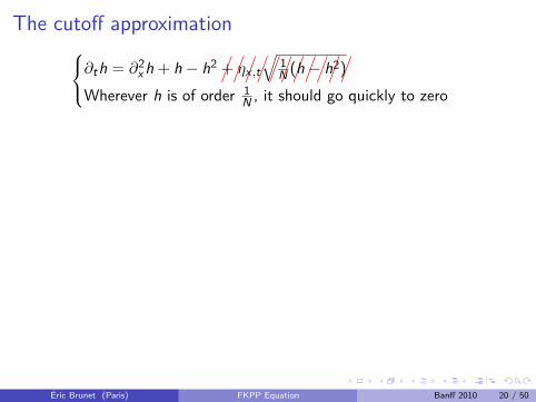
The cutoff approximation∂th = ∂2x h + h − h2///////////+ ηx ,t
√1N (h − h2)
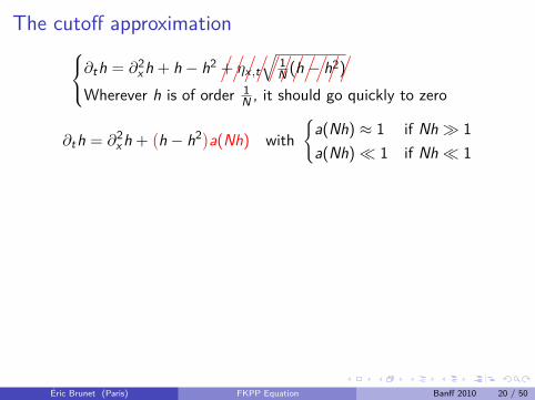
Wherever h is of order 1N , it should go quickly to zero
∂th = ∂2x h +(h − h2
)a(Nh) with
{a(Nh) ≈ 1 if Nh� 1a(Nh)� 1 if Nh� 1
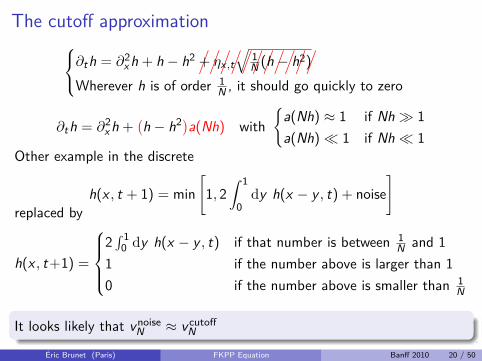
Other example in the discrete
h(x , t + 1) = min[1, 2
∫ 1
0dy h(x − y , t) + noise
]replaced by
h(x , t+1) =
2∫ 10 dy h(x − y , t) if that number is between 1
N and 11 if the number above is larger than 10 if the number above is smaller than 1
N
It looks likely that vnoiseN ≈ v cutoff
N
Éric Brunet (Paris) FKPP Equation Banff 2010 20 / 50
The cutoff approximation∂th = ∂2x h + h − h2///////////+ ηx ,t
√1N (h − h2)
Wherever h is of order 1N , it should go quickly to zero
∂th = ∂2x h +(h − h2
)a(Nh) with
{a(Nh) ≈ 1 if Nh� 1a(Nh)� 1 if Nh� 1
Other example in the discrete
h(x , t + 1) = min[1, 2
∫ 1
0dy h(x − y , t) + noise
]replaced by
h(x , t+1) =
2∫ 10 dy h(x − y , t) if that number is between 1
N and 11 if the number above is larger than 10 if the number above is smaller than 1
N
It looks likely that vnoiseN ≈ v cutoff
N
Éric Brunet (Paris) FKPP Equation Banff 2010 20 / 50
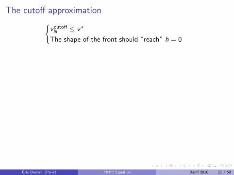
The cutoff approximation{v cutoff
N ≤ v∗
The shape of the front should “reach” h = 0
γ = γR + iγI v = v(γ) (real)
fv (z) = C sin(γIz
//
+ φ)e−γRz
Let L� 1 the value of z where thecutoff happens
γIL ≈ π e−γRL ≈ 1N
γI � 1 =⇒ γR ≈ γ∗ to have v(γ) real
L ≈ lnNγ∗
fv (z) ≈ ALπ
sin(πzL
)e−γ∗z
Éric Brunet (Paris) FKPP Equation Banff 2010 21 / 50
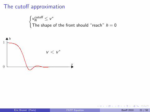
The cutoff approximation{v cutoff
N ≤ v∗
The shape of the front should “reach” h = 0
v < v ∗
x
h1
0
γ = γR + iγI v = v(γ) (real)
fv (z) = C sin(γIz
//
+ φ)e−γRz
Let L� 1 the value of z where thecutoff happens
γIL ≈ π e−γRL ≈ 1N
γI � 1 =⇒ γR ≈ γ∗ to have v(γ) real
L ≈ lnNγ∗
fv (z) ≈ ALπ
sin(πzL
)e−γ∗z
Éric Brunet (Paris) FKPP Equation Banff 2010 21 / 50

The cutoff approximation{v cutoff
N ≤ v∗
The shape of the front should “reach” h = 0
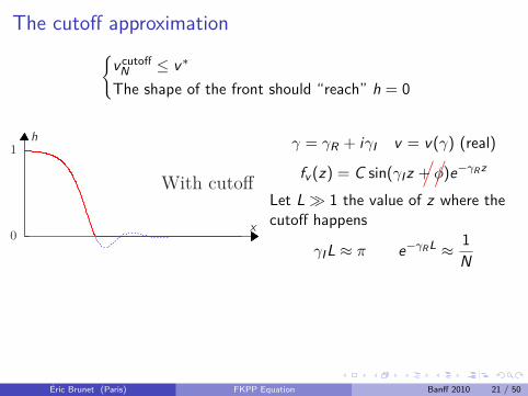
With cutoff
x
h1
0
γ = γR + iγI v = v(γ) (real)
fv (z) = C sin(γIz
//
+ φ)e−γRz
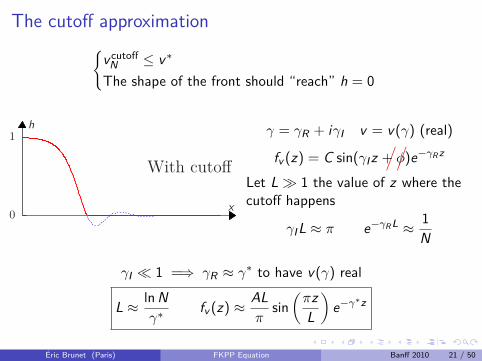
Let L� 1 the value of z where thecutoff happens
γIL ≈ π e−γRL ≈ 1N
γI � 1 =⇒ γR ≈ γ∗ to have v(γ) real
L ≈ lnNγ∗
fv (z) ≈ ALπ
sin(πzL
)e−γ∗z
Éric Brunet (Paris) FKPP Equation Banff 2010 21 / 50

The cutoff approximation{v cutoff
N ≤ v∗
The shape of the front should “reach” h = 0
With cutoff
x
h1
0
γ = γR + iγI v = v(γ) (real)
fv (z) = C sin(γIz
//
+ φ)e−γRz
Let L� 1 the value of z where thecutoff happens
γIL ≈ π e−γRL ≈ 1N
γI � 1 =⇒ γR ≈ γ∗ to have v(γ) real
L ≈ lnNγ∗
fv (z) ≈ ALπ
sin(πzL
)e−γ∗z
Éric Brunet (Paris) FKPP Equation Banff 2010 21 / 50

The cutoff approximation{v cutoff
N ≤ v∗
The shape of the front should “reach” h = 0
With cutoff
x
h1
0
γ = γR + iγI v = v(γ) (real)
fv (z) = C sin(γIz//
+ φ)e−γRz
Let L� 1 the value of z where thecutoff happens
γIL ≈ π e−γRL ≈ 1N
γI � 1 =⇒ γR ≈ γ∗ to have v(γ) real
L ≈ lnNγ∗
fv (z) ≈ ALπ
sin(πzL
)e−γ∗z
Éric Brunet (Paris) FKPP Equation Banff 2010 21 / 50
The cutoff approximation
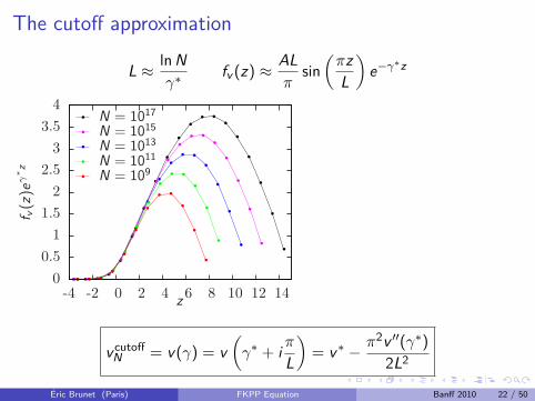
L ≈ lnNγ∗
fv (z) ≈ ALπ
sin(πzL
)e−γ∗z
N = 109N = 1011N = 1013N = 1015N = 1017
z
f v(z
)eγ∗ z
14121086420-2-4
43.5
32.5
21.5
10.5
0
v cutoffN = v(γ) = v
(γ∗ + i πL
)= v∗ − π2v ′′(γ∗)
2L2
Éric Brunet (Paris) FKPP Equation Banff 2010 22 / 50
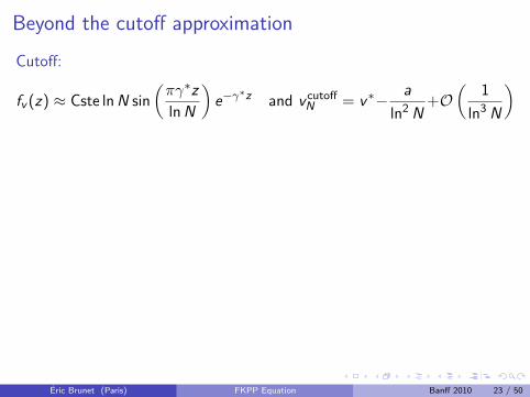
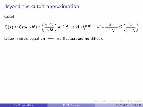
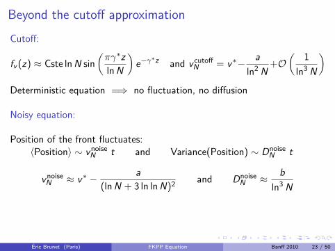
Beyond the cutoff approximationCutoff:
fv (z) ≈ Cste lnN sin(πγ∗zlnN
)e−γ∗z and v cutoff
N = v∗− aln2 N
+O( 1ln3 N
)
Deterministic equation =⇒ no fluctuation, no diffusion
Noisy equation:
Position of the front fluctuates:〈Position〉 ∼ vnoise
N t and Variance(Position) ∼ DnoiseN t
vnoiseN ≈ v∗ − a
(lnN + 3 ln lnN)2and Dnoise
N ≈ bln3 N
with a =π2γ∗2v ′′(γ∗)
2 b =π4γ∗v ′′(γ∗)
3
Éric Brunet (Paris) FKPP Equation Banff 2010 23 / 50
Beyond the cutoff approximationCutoff:
fv (z) ≈ Cste lnN sin(πγ∗zlnN
)e−γ∗z and v cutoff
N = v∗− aln2 N
+O( 1ln3 N
)Deterministic equation =⇒ no fluctuation, no diffusion
Noisy equation:
Position of the front fluctuates:〈Position〉 ∼ vnoise
N t and Variance(Position) ∼ DnoiseN t
vnoiseN ≈ v∗ − a
(lnN + 3 ln lnN)2and Dnoise
N ≈ bln3 N
with a =π2γ∗2v ′′(γ∗)
2 b =π4γ∗v ′′(γ∗)
3
Éric Brunet (Paris) FKPP Equation Banff 2010 23 / 50
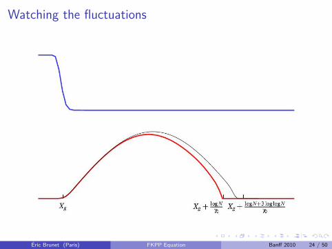
Watching the fluctuations
Éric Brunet (Paris) FKPP Equation Banff 2010 24 / 50

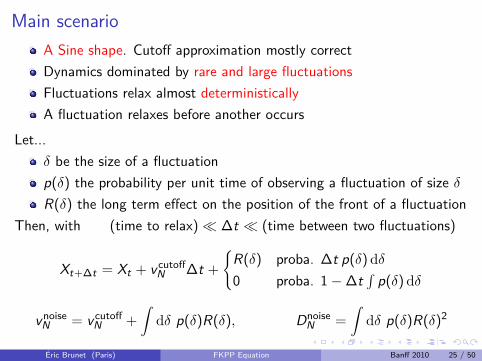
Main scenarioA Sine shape. Cutoff approximation mostly correct
Dynamics dominated by rare and large fluctuationsFluctuations relax almost deterministicallyA fluctuation relaxes before another occurs
Let...δ be the size of a fluctuationp(δ) the probability per unit time of observing a fluctuation of size δR(δ) the long term effect on the position of the front of a fluctuation
Then, with (time to relax)� ∆t � (time between two fluctuations)
Xt+∆t = Xt + v cutoffN ∆t +
{R(δ) proba. ∆t p(δ) dδ0 proba. 1−∆t
∫p(δ) dδ
vnoiseN = v cutoff
N +
∫dδ p(δ)R(δ), Dnoise
N =
∫dδ p(δ)R(δ)2
Éric Brunet (Paris) FKPP Equation Banff 2010 25 / 50
Main scenarioA Sine shape. Cutoff approximation mostly correctDynamics dominated by rare and large fluctuations
Fluctuations relax almost deterministicallyA fluctuation relaxes before another occurs
Let...δ be the size of a fluctuationp(δ) the probability per unit time of observing a fluctuation of size δR(δ) the long term effect on the position of the front of a fluctuation
Then, with (time to relax)� ∆t � (time between two fluctuations)
Xt+∆t = Xt + v cutoffN ∆t +
{R(δ) proba. ∆t p(δ) dδ0 proba. 1−∆t
∫p(δ) dδ
vnoiseN = v cutoff
N +
∫dδ p(δ)R(δ), Dnoise
N =
∫dδ p(δ)R(δ)2
Éric Brunet (Paris) FKPP Equation Banff 2010 25 / 50

Main scenarioA Sine shape. Cutoff approximation mostly correctDynamics dominated by rare and large fluctuationsFluctuations relax almost deterministically
A fluctuation relaxes before another occursLet...
δ be the size of a fluctuationp(δ) the probability per unit time of observing a fluctuation of size δR(δ) the long term effect on the position of the front of a fluctuation
Then, with (time to relax)� ∆t � (time between two fluctuations)
Xt+∆t = Xt + v cutoffN ∆t +
{R(δ) proba. ∆t p(δ) dδ0 proba. 1−∆t
∫p(δ) dδ
vnoiseN = v cutoff
N +
∫dδ p(δ)R(δ), Dnoise
N =
∫dδ p(δ)R(δ)2
Éric Brunet (Paris) FKPP Equation Banff 2010 25 / 50
Main scenarioA Sine shape. Cutoff approximation mostly correctDynamics dominated by rare and large fluctuationsFluctuations relax almost deterministicallyA fluctuation relaxes before another occurs
Let...δ be the size of a fluctuationp(δ) the probability per unit time of observing a fluctuation of size δR(δ) the long term effect on the position of the front of a fluctuation
Then, with (time to relax)� ∆t � (time between two fluctuations)
Xt+∆t = Xt + v cutoffN ∆t +
{R(δ) proba. ∆t p(δ) dδ0 proba. 1−∆t
∫p(δ) dδ
vnoiseN = v cutoff
N +
∫dδ p(δ)R(δ), Dnoise
N =
∫dδ p(δ)R(δ)2
Éric Brunet (Paris) FKPP Equation Banff 2010 25 / 50
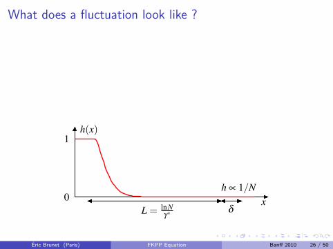
What does a fluctuation look like ?
0
1h(x)
xδL = lnN
γ∗
h ∝ 1/N0
Nh(x)
xδL = lnN
γ∗
h ∝ 1/N
0
1h(x)
xδL = lnN
γ∗
h ∝ 1/N
Éric Brunet (Paris) FKPP Equation Banff 2010 26 / 50

What does a fluctuation look like ?
0
1h(x)
xδL = lnN
γ∗
h ∝ 1/N
0
Nh(x)
xδL = lnN
γ∗
h ∝ 1/N
0
Nh(x)
xδL = lnN
γ∗
h ∝ 1/N
Éric Brunet (Paris) FKPP Equation Banff 2010 26 / 50

What does a fluctuation look like ?
0
1h(x)
xδL = lnN
γ∗
h ∝ 1/N0
Nh(x)
xδL = lnN
γ∗
h ∝ 1/N
0
h(x)eγ∗x
xδL = lnN
γ∗
Éric Brunet (Paris) FKPP Equation Banff 2010 26 / 50
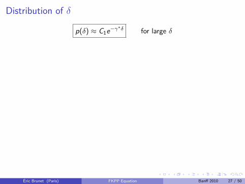
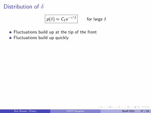
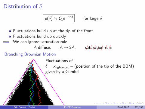
Distribution of δ
p(δ) ≈ C1e−γ∗δ for large δ
Fluctuations build up at the tip of the frontFluctuations build up quickly
=⇒ We can ignore saturation ruleA diffuse, A→ 2A,
/ / / / / / /saturation rule
Branching Brownian MotionFluctuations ofδ = xrightmost − (position of the tip of the BBM)given by a Gumbel
Éric Brunet (Paris) FKPP Equation Banff 2010 27 / 50

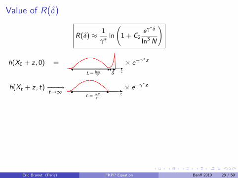
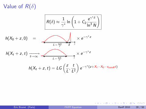
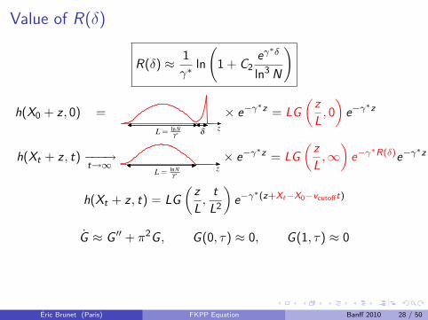
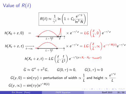
Value of R(δ)
R(δ) ≈ 1γ∗
ln(1 + C2
eγ∗δ
ln3 N
)
h(X0 + z , 0) =z
δL = lnNγ∗
× e−γ∗z
= LG(z
L , 0)
e−γ∗z
h(Xt + z , t) −−−→t→∞ zL = lnN
γ∗
× e−γ∗z
= LG(z
L ,∞)
e−γ∗R(δ)e−γ∗z
h(Xt + z , t) = LG(z
L ,tL2)
e−γ∗(z+Xt−X0−vcutofft)
G ≈ G ′′ + π2G , G(0, τ) ≈ 0, G(1, τ) ≈ 0
G(y , 0) = sin(πy) + perturbation of width ∝ 1L and height ∝ eγ∗δ
LG(y ,∞) = sin(πy)eγ∗R(δ) eγ∗R(δ) = 2
∫ 1
0dy sin(πy)G(y , 0)
Éric Brunet (Paris) FKPP Equation Banff 2010 28 / 50
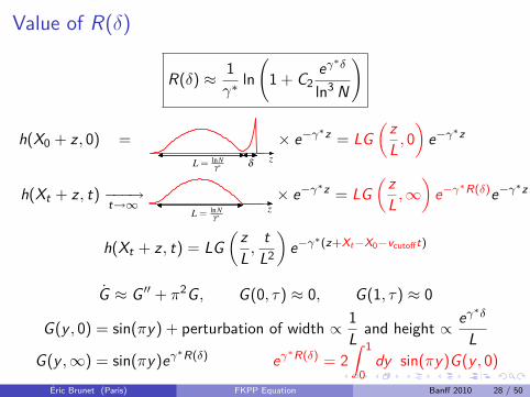

Value of R(δ)
R(δ) ≈ 1γ∗
ln(1 + C2
eγ∗δ
ln3 N
)
h(X0 + z , 0) =z
δL = lnNγ∗
× e−γ∗z = LG(z
L , 0)
e−γ∗z
h(Xt + z , t) −−−→t→∞ zL = lnN
γ∗
× e−γ∗z = LG(z
L ,∞)
e−γ∗R(δ)e−γ∗z
h(Xt + z , t) = LG(z
L ,tL2)
e−γ∗(z+Xt−X0−vcutofft)
G ≈ G ′′ + π2G , G(0, τ) ≈ 0, G(1, τ) ≈ 0
G(y , 0) = sin(πy) + perturbation of width ∝ 1L and height ∝ eγ∗δ
LG(y ,∞) = sin(πy)eγ∗R(δ) eγ∗R(δ) = 2
∫ 1
0dy sin(πy)G(y , 0)
Éric Brunet (Paris) FKPP Equation Banff 2010 28 / 50
Value of R(δ)
R(δ) ≈ 1γ∗
ln(1 + C2
eγ∗δ
ln3 N
)
h(X0 + z , 0) =z
δL = lnNγ∗
× e−γ∗z = LG(z
L , 0)
e−γ∗z
h(Xt + z , t) −−−→t→∞ zL = lnN
γ∗
× e−γ∗z = LG(z
L ,∞)
e−γ∗R(δ)e−γ∗z
h(Xt + z , t) = LG(z
L ,tL2)
e−γ∗(z+Xt−X0−vcutofft)
G ≈ G ′′ + π2G , G(0, τ) ≈ 0, G(1, τ) ≈ 0
G(y , 0) = sin(πy) + perturbation of width ∝ 1L and height ∝ eγ∗δ
LG(y ,∞) = sin(πy)eγ∗R(δ)
eγ∗R(δ) = 2∫ 1
0dy sin(πy)G(y , 0)
Éric Brunet (Paris) FKPP Equation Banff 2010 28 / 50
Value of R(δ)
R(δ) ≈ 1γ∗
ln(1 + C2
eγ∗δ
ln3 N
)
h(X0 + z , 0) =z
δL = lnNγ∗
× e−γ∗z = LG(z
L , 0)
e−γ∗z
h(Xt + z , t) −−−→t→∞ zL = lnN
γ∗
× e−γ∗z = LG(z
L ,∞)
e−γ∗R(δ)e−γ∗z
h(Xt + z , t) = LG(z
L ,tL2)
e−γ∗(z+Xt−X0−vcutofft)
G ≈ G ′′ + π2G , G(0, τ) ≈ 0, G(1, τ) ≈ 0
G(y , 0) = sin(πy) + perturbation of width ∝ 1L and height ∝ eγ∗δ
LG(y ,∞) = sin(πy)eγ∗R(δ) eγ∗R(δ) = 2
∫ 1
0dy sin(πy)G(y , 0)
Éric Brunet (Paris) FKPP Equation Banff 2010 28 / 50
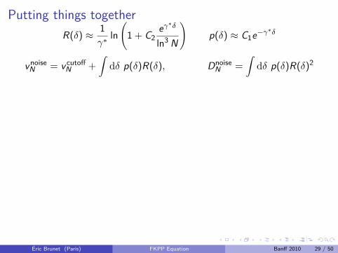
Putting things togetherR(δ) ≈ 1
γ∗ln(1 + C2
eγ∗δ
ln3 N
)p(δ) ≈ C1e−γ
∗δ
vnoiseN = v cutoff
N +
∫dδ p(δ)R(δ), Dnoise
N =
∫dδ p(δ)R(δ)2
This givesvnoise
N ≈ v cutoffN +
C1C2γ∗2
3 ln lnNln3 N
, DnoiseN ≈ C1C2
γ∗3π2
3 ln3 NTimescales
Relevant values of δ are ≈ 1γ∗ 3 ln lnN
Time between two relevant fluctuations is ln3 NRelaxation time is ln2 N
C1C2 ?
Cutoff theory gives v = v∗ − π2v ′′(γ∗)2L2 with L = 1
γ∗ lnN
Use instead the effective length L = 1γ∗ [lnN + 3 ln lnN]
Éric Brunet (Paris) FKPP Equation Banff 2010 29 / 50
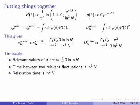
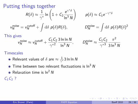
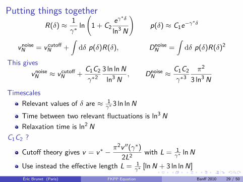
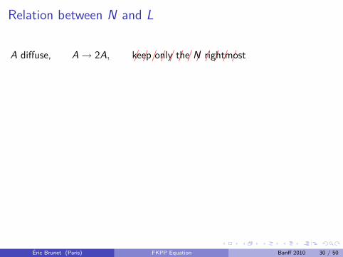
Relation between N and L
A diffuse, A→ 2A,/ / / / / / / / / / / /keep only the N rightmost
a wall moving at velocity v absorbs the particles
replaced by������������������������������������������������
������������������������������������������������
vwall = 2− π2
L2
Start with one particle at x > 0Condition on the fact that thereis one living particle at largetime THow many particles at anintermediate time ?
Starts with a density looking likethe actual front
h(x , 0) ∝ L sin πxL e−x
Populate with N particlesProba to survive
∼ 1− e−KNL3e−L
L ≈ lnN + 3 ln lnN
Éric Brunet (Paris) FKPP Equation Banff 2010 30 / 50
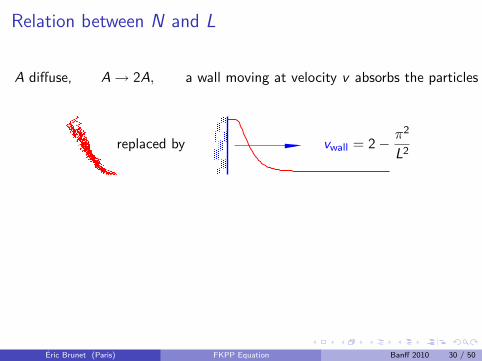
Relation between N and L
A diffuse, A→ 2A, a wall moving at velocity v absorbs the particles
replaced by������������������������������������������������
������������������������������������������������
vwall = 2− π2
L2
Start with one particle at x > 0Condition on the fact that thereis one living particle at largetime THow many particles at anintermediate time ?
Starts with a density looking likethe actual front
h(x , 0) ∝ L sin πxL e−x
Populate with N particlesProba to survive
∼ 1− e−KNL3e−L
L ≈ lnN + 3 ln lnN
Éric Brunet (Paris) FKPP Equation Banff 2010 30 / 50
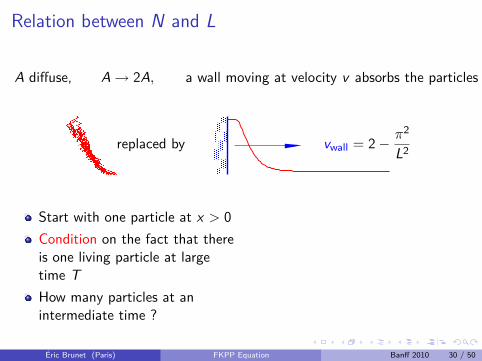
Relation between N and L
A diffuse, A→ 2A, a wall moving at velocity v absorbs the particles
replaced by������������������������������������������������
������������������������������������������������
vwall = 2− π2
L2
Start with one particle at x > 0Condition on the fact that thereis one living particle at largetime THow many particles at anintermediate time ?
Starts with a density looking likethe actual front
h(x , 0) ∝ L sin πxL e−x
Populate with N particlesProba to survive
∼ 1− e−KNL3e−L
L ≈ lnN + 3 ln lnNÉric Brunet (Paris) FKPP Equation Banff 2010 30 / 50
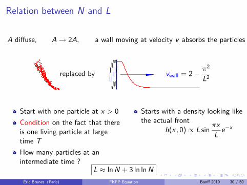
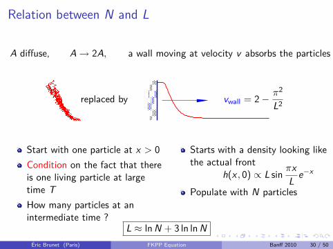
Relation between N and L
A diffuse, A→ 2A, a wall moving at velocity v absorbs the particles
replaced by������������������������������������������������
������������������������������������������������
vwall = 2− π2
L2
Start with one particle at x > 0Condition on the fact that thereis one living particle at largetime THow many particles at anintermediate time ?
Starts with a density looking likethe actual front
h(x , 0) ∝ L sin πxL e−x
Populate with N particles
Proba to survive
∼ 1− e−KNL3e−L
L ≈ lnN + 3 ln lnNÉric Brunet (Paris) FKPP Equation Banff 2010 30 / 50

Relation between N and L
A diffuse, A→ 2A, a wall moving at velocity v absorbs the particles
replaced by������������������������������������������������
������������������������������������������������
vwall = 2− π2
L2
Start with one particle at x > 0Condition on the fact that thereis one living particle at largetime THow many particles at anintermediate time ?
Starts with a density looking likethe actual front
h(x , 0) ∝ L sin πxL e−x
Populate with N particlesProba to survive
∼ 1− e−KNL3e−L
L ≈ lnN + 3 ln lnNÉric Brunet (Paris) FKPP Equation Banff 2010 30 / 50
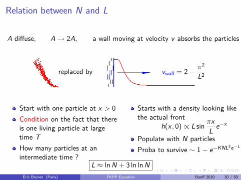
Relation between N and L
A diffuse, A→ 2A, a wall moving at velocity v absorbs the particles
replaced by������������������������������������������������
������������������������������������������������
vwall = 2− π2
L2
Start with one particle at x > 0Condition on the fact that thereis one living particle at largetime THow many particles at anintermediate time ?
Starts with a density looking likethe actual front
h(x , 0) ∝ L sin πxL e−x
Populate with N particlesProba to survive ∼ 1− e−KNL3e−L
L ≈ lnN + 3 ln lnNÉric Brunet (Paris) FKPP Equation Banff 2010 30 / 50
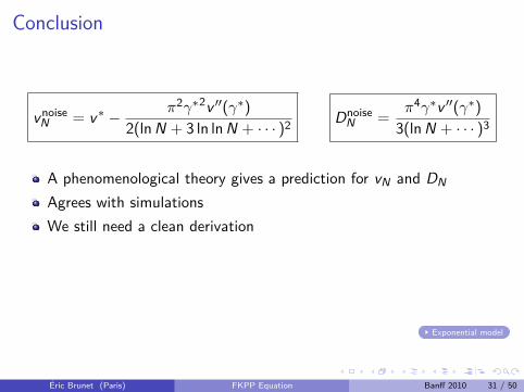
Conclusion
vnoiseN = v∗ − π2γ∗2v ′′(γ∗)
2(lnN + 3 ln lnN + · · · )2 DnoiseN =
π4γ∗v ′′(γ∗)3(lnN + · · · )3
A phenomenological theory gives a prediction for vN and DN
Agrees with simulationsWe still need a clean derivation
Exponential model
Éric Brunet (Paris) FKPP Equation Banff 2010 31 / 50
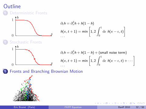
Outline1 Deterministic Fronts
x
h1
0
∂th = ∂2x h + h(1− h)
h(x , t + 1) = min[
1, 2∫ 1
0dε h(x − ε, t)
]. . .
2 Stochastic Fronts
x
h1
0
∂th = ∂2x h + h(1− h) + (small noise term)
h(x , t + 1) = min[
1, 2∫ 1
0dε h(x − ε, t) + · · ·
]. . .
3 Fronts and Branching Brownian Motion
Éric Brunet (Paris) FKPP Equation Banff 2010 32 / 50
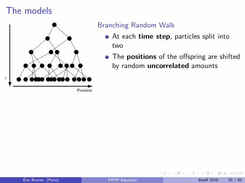
The models
Position
t
Branching Random WalkAt each time step, particles split intotwoThe positions of the offspring are shiftedby random uncorrelated amounts
Branching Brownian MotionParticles do a Brownian motionWith rate 1, they split
Also: directed polymer on a Caley tree,evolution,GREM (?)
Positions of the rightmost particles ? (Energy spectrum ?)
Éric Brunet (Paris) FKPP Equation Banff 2010 33 / 50
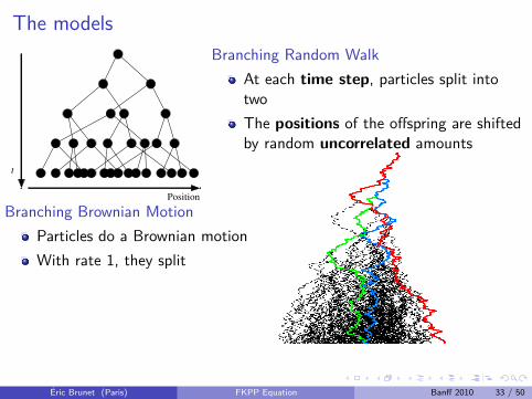
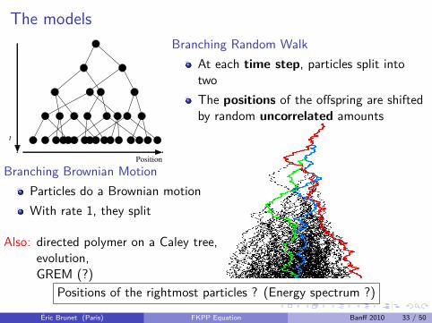
The models
Position
t
Branching Random WalkAt each time step, particles split intotwoThe positions of the offspring are shiftedby random uncorrelated amounts
Branching Brownian MotionParticles do a Brownian motionWith rate 1, they split
Also: directed polymer on a Caley tree,evolution,GREM (?)
Positions of the rightmost particles ? (Energy spectrum ?)Éric Brunet (Paris) FKPP Equation Banff 2010 33 / 50
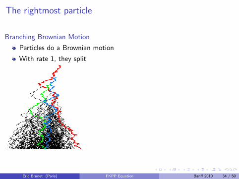
The rightmost particle
Branching Brownian MotionParticles do a Brownian motionWith rate 1, they split
Distribution of the rightmost
Q0(x , t) = Proba[X1(t) < x ]
Q0(x , t) =
(〈X1(t)〉
1
0
)
∂tQ0 = ∂2x Q0 − Q0 + Q02
Q0(x , 0) =
(0
0
1)
FKPP equation! (h = 1− Q)Position of the rightmost
X1(t) = 2t − 32 ln t +O(1)
Éric Brunet (Paris) FKPP Equation Banff 2010 34 / 50
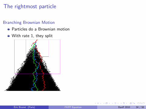
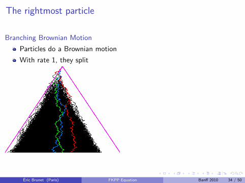
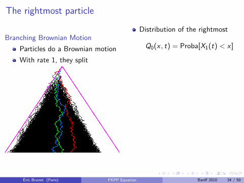

The rightmost particle
Branching Brownian MotionParticles do a Brownian motionWith rate 1, they split
Distribution of the rightmost
Q0(x , t) = Proba[X1(t) < x ]
Q0(x , t) =
(〈X1(t)〉
1
0
)
∂tQ0 = ∂2x Q0 − Q0 + Q02
Q0(x , 0) =
(0
0
1)
FKPP equation! (h = 1− Q)
Position of the rightmost
X1(t) = 2t − 32 ln t +O(1)
Éric Brunet (Paris) FKPP Equation Banff 2010 34 / 50

The rightmost particle
Branching Brownian MotionParticles do a Brownian motionWith rate 1, they split
Distribution of the rightmost
Q0(x , t) = Proba[X1(t) < x ]
Q0(x , t) =
(〈X1(t)〉
1
0
)
∂tQ0 = ∂2x Q0 − Q0 + Q02
Q0(x , 0) =
(0
0
1)
FKPP equation! (h = 1− Q)Position of the rightmost
X1(t) = 2t − 32 ln t +O(1)
Éric Brunet (Paris) FKPP Equation Banff 2010 34 / 50
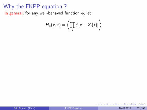
Why the FKPP equation ?In general, for any well-behaved function φ, let
Hφ(x , t) =
⟨∏iφ[x − Xi (t)]
⟩
What does happen between times 0 and dt ?
Hφ(x , t + dt) =⟨
(1− dt)Hφ
(x − η
√2dt, t
)⟩η︸ ︷︷ ︸
the initial particle did not branch
+ dt Hφ(x , t)2︸ ︷︷ ︸the initial particle did branch
∂tHφ = ∂2x Hφ − Hφ + H2φ Hφ(x , 0) = φ(x)
For φ(x) =
(0
0
1), Hφ is the probability Q0 that all the
particles are on the left of x
Hφ(Xt +z , t)→ F2(z) with Xt = 2t− 32 ln t +a0− 3√π√
t+
a1t +
a3/2t3/2 + · · ·
For φ(x) =
(0
1
0
), Hφ(Xt + z , t)→ F2(z),
Hφ(Xt + z , t)→ F2(z + δ[φ])
Éric Brunet (Paris) FKPP Equation Banff 2010 35 / 50
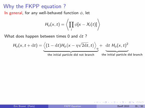

Why the FKPP equation ?In general, for any well-behaved function φ, let
Hφ(x , t) =
⟨∏iφ[x − Xi (t)]
⟩
What does happen between times 0 and dt ?
Hφ(x , t + dt) =⟨
(1− dt)Hφ
(x − η
√2dt, t
)⟩η︸ ︷︷ ︸
the initial particle did not branch
+ dt Hφ(x , t)2︸ ︷︷ ︸the initial particle did branch
∂tHφ = ∂2x Hφ − Hφ + H2φ
Hφ(x , 0) = φ(x)
For φ(x) =
(0
0
1), Hφ is the probability Q0 that all the
particles are on the left of x
Hφ(Xt +z , t)→ F2(z) with Xt = 2t− 32 ln t +a0− 3√π√
t+
a1t +
a3/2t3/2 + · · ·
For φ(x) =
(0
1
0
), Hφ(Xt + z , t)→ F2(z),
Hφ(Xt + z , t)→ F2(z + δ[φ])
Éric Brunet (Paris) FKPP Equation Banff 2010 35 / 50

Why the FKPP equation ?In general, for any well-behaved function φ, let
Hφ(x , t) =
⟨∏iφ[x − Xi (t)]
⟩
What does happen between times 0 and dt ?
Hφ(x , t + dt) =⟨
(1− dt)Hφ
(x − η
√2dt, t
)⟩η︸ ︷︷ ︸
the initial particle did not branch
+ dt Hφ(x , t)2︸ ︷︷ ︸the initial particle did branch
∂tHφ = ∂2x Hφ − Hφ + H2φ Hφ(x , 0) = φ(x)
For φ(x) =
(0
0
1), Hφ is the probability Q0 that all the
particles are on the left of x
Hφ(Xt +z , t)→ F2(z) with Xt = 2t− 32 ln t +a0− 3√π√
t+
a1t +
a3/2t3/2 + · · ·
For φ(x) =
(0
1
0
), Hφ(Xt + z , t)→ F2(z),
Hφ(Xt + z , t)→ F2(z + δ[φ])
Éric Brunet (Paris) FKPP Equation Banff 2010 35 / 50
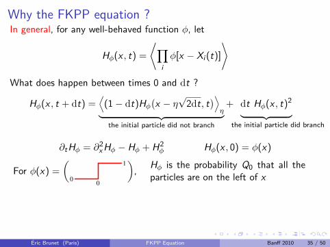
Why the FKPP equation ?In general, for any well-behaved function φ, let
Hφ(x , t) =
⟨∏iφ[x − Xi (t)]
⟩
What does happen between times 0 and dt ?
Hφ(x , t + dt) =⟨
(1− dt)Hφ
(x − η
√2dt, t
)⟩η︸ ︷︷ ︸
the initial particle did not branch
+ dt Hφ(x , t)2︸ ︷︷ ︸the initial particle did branch
∂tHφ = ∂2x Hφ − Hφ + H2φ Hφ(x , 0) = φ(x)
For φ(x) =
(0
0
1), Hφ is the probability Q0 that all the
particles are on the left of x
Hφ(Xt +z , t)→ F2(z) with Xt = 2t− 32 ln t +a0− 3√π√
t+
a1t +
a3/2t3/2 + · · ·
For φ(x) =
(0
1
0
), Hφ(Xt + z , t)→ F2(z),
Hφ(Xt + z , t)→ F2(z + δ[φ])
Éric Brunet (Paris) FKPP Equation Banff 2010 35 / 50
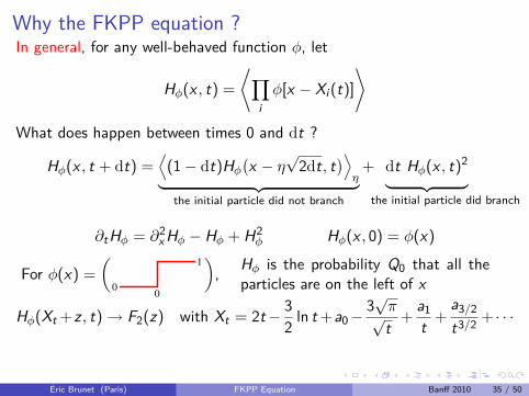
Why the FKPP equation ?In general, for any well-behaved function φ, let
Hφ(x , t) =
⟨∏iφ[x − Xi (t)]
⟩
What does happen between times 0 and dt ?
Hφ(x , t + dt) =⟨
(1− dt)Hφ
(x − η
√2dt, t
)⟩η︸ ︷︷ ︸
the initial particle did not branch
+ dt Hφ(x , t)2︸ ︷︷ ︸the initial particle did branch
∂tHφ = ∂2x Hφ − Hφ + H2φ Hφ(x , 0) = φ(x)
For φ(x) =
(0
0
1), Hφ is the probability Q0 that all the
particles are on the left of x
Hφ(Xt +z , t)→ F2(z) with Xt = 2t− 32 ln t +a0− 3√π√
t+
a1t +
a3/2t3/2 + · · ·
For φ(x) =
(0
1
0
),
Hφ(Xt + z , t)→ F2(z),Hφ(Xt + z , t)→ F2(z + δ[φ])
Éric Brunet (Paris) FKPP Equation Banff 2010 35 / 50
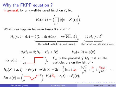
Why the FKPP equation ?In general, for any well-behaved function φ, let
Hφ(x , t) =
⟨∏iφ[x − Xi (t)]
⟩
What does happen between times 0 and dt ?
Hφ(x , t + dt) =⟨
(1− dt)Hφ
(x − η
√2dt, t
)⟩η︸ ︷︷ ︸
the initial particle did not branch
+ dt Hφ(x , t)2︸ ︷︷ ︸the initial particle did branch
∂tHφ = ∂2x Hφ − Hφ + H2φ Hφ(x , 0) = φ(x)
For φ(x) =
(0
0
1), Hφ is the probability Q0 that all the
particles are on the left of x
Hφ(Xt +z , t)→ F2(z) with Xt = 2t− 32 ln t +a0− 3√π√
t+
a1t +
a3/2t3/2 + · · ·
For φ(x) =
(0
1
0
), Hφ(Xt + z , t)→ F2(z),
Hφ(Xt + z , t)→ F2(z + δ[φ])
Éric Brunet (Paris) FKPP Equation Banff 2010 35 / 50
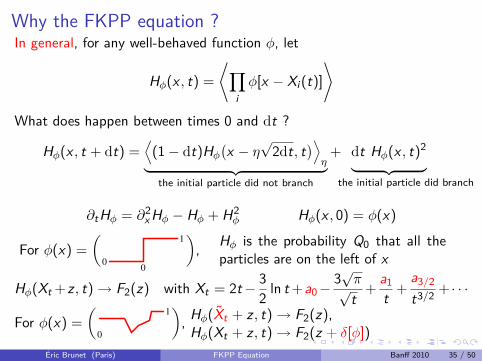
Why the FKPP equation ?In general, for any well-behaved function φ, let
Hφ(x , t) =
⟨∏iφ[x − Xi (t)]
⟩
What does happen between times 0 and dt ?
Hφ(x , t + dt) =⟨
(1− dt)Hφ
(x − η
√2dt, t
)⟩η︸ ︷︷ ︸
the initial particle did not branch
+ dt Hφ(x , t)2︸ ︷︷ ︸the initial particle did branch
∂tHφ = ∂2x Hφ − Hφ + H2φ Hφ(x , 0) = φ(x)
For φ(x) =
(0
0
1), Hφ is the probability Q0 that all the
particles are on the left of x
Hφ(Xt +z , t)→ F2(z) with Xt = 2t− 32 ln t +a0− 3√π√
t+
a1t +
a3/2t3/2 + · · ·
For φ(x) =
(0
1
0
), Hφ(Xt + z , t)→ F2(z),
Hφ(Xt + z , t)→ F2(z + δ[φ])
Éric Brunet (Paris) FKPP Equation Banff 2010 35 / 50
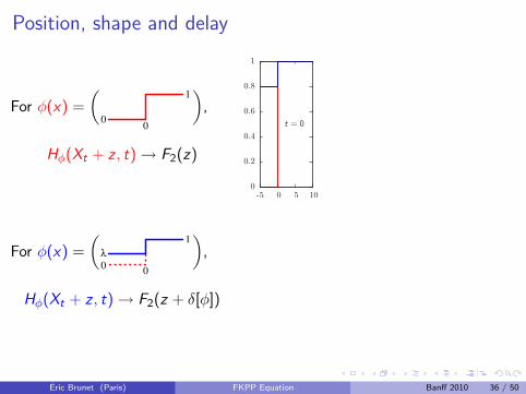
Position, shape and delay
For φ(x) =
(0
0
1),
Hφ(Xt + z , t)→ F2(z)
For φ(x) =
(0
1
0
λ
),
Hφ(Xt + z , t)→ F2(z + δ[φ])
t = 0
1050-5
1
0.8
0.6
0.4
0.2
0
t = 20t = 10t = 5
454035302520151050-5
1
0.8
0.6
0.4
0.2
0
Éric Brunet (Paris) FKPP Equation Banff 2010 36 / 50
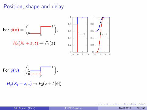
Position, shape and delay
For φ(x) =
(0
0
1),
Hφ(Xt + z , t)→ F2(z)
For φ(x) =
(0
1
0
λ
),
Hφ(Xt + z , t)→ F2(z + δ[φ])
t = 0
1050-5
1
0.8
0.6
0.4
0.2
0
t = 1
1050-5
1
0.8
0.6
0.4
0.2
0
t = 20t = 10t = 5
454035302520151050-5
1
0.8
0.6
0.4
0.2
0
Éric Brunet (Paris) FKPP Equation Banff 2010 36 / 50
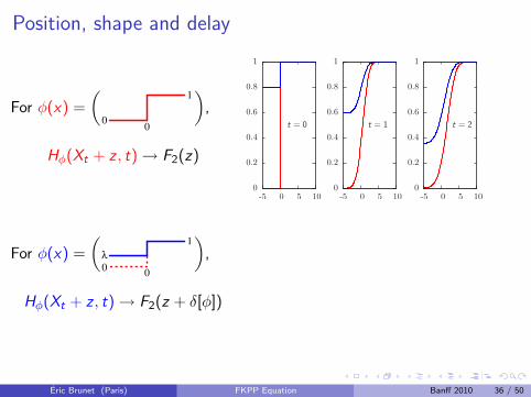
Position, shape and delay
For φ(x) =
(0
0
1),
Hφ(Xt + z , t)→ F2(z)
For φ(x) =
(0
1
0
λ
),
Hφ(Xt + z , t)→ F2(z + δ[φ])
t = 0
1050-5
1
0.8
0.6
0.4
0.2
0
t = 1
1050-5
1
0.8
0.6
0.4
0.2
0
t = 2
1050-5
1
0.8
0.6
0.4
0.2
0
t = 20t = 10t = 5
454035302520151050-5
1
0.8
0.6
0.4
0.2
0
Éric Brunet (Paris) FKPP Equation Banff 2010 36 / 50

Position, shape and delay
For φ(x) =
(0
0
1),
Hφ(Xt + z , t)→ F2(z)
For φ(x) =
(0
1
0
λ
),
Hφ(Xt + z , t)→ F2(z + δ[φ])
t = 0
1050-5
1
0.8
0.6
0.4
0.2
0
t = 1
1050-5
1
0.8
0.6
0.4
0.2
0
t = 2
1050-5
1
0.8
0.6
0.4
0.2
0
t = 5
454035302520151050-5
1
0.8
0.6
0.4
0.2
0
t = 20t = 10t = 5
454035302520151050-5
1
0.8
0.6
0.4
0.2
0
Éric Brunet (Paris) FKPP Equation Banff 2010 36 / 50
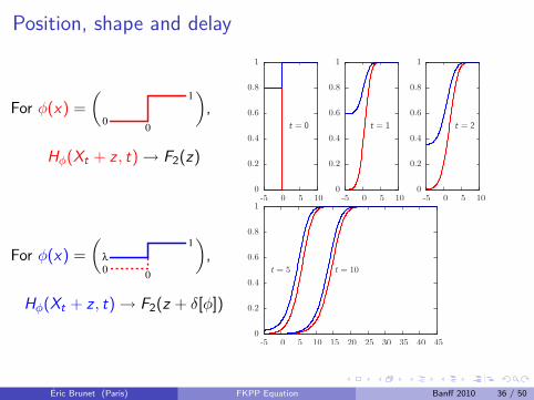
Position, shape and delay
For φ(x) =
(0
0
1),
Hφ(Xt + z , t)→ F2(z)
For φ(x) =
(0
1
0
λ
),
Hφ(Xt + z , t)→ F2(z + δ[φ])
t = 0
1050-5
1
0.8
0.6
0.4
0.2
0
t = 1
1050-5
1
0.8
0.6
0.4
0.2
0
t = 2
1050-5
1
0.8
0.6
0.4
0.2
0
t = 10t = 5
454035302520151050-5
1
0.8
0.6
0.4
0.2
0
t = 20t = 10t = 5
454035302520151050-5
1
0.8
0.6
0.4
0.2
0
Éric Brunet (Paris) FKPP Equation Banff 2010 36 / 50
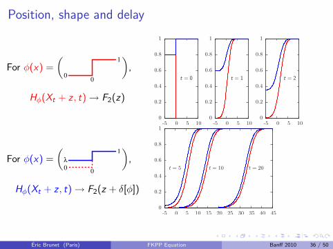
Position, shape and delay
For φ(x) =
(0
0
1),
Hφ(Xt + z , t)→ F2(z)
For φ(x) =
(0
1
0
λ
),
Hφ(Xt + z , t)→ F2(z + δ[φ])
t = 0
1050-5
1
0.8
0.6
0.4
0.2
0
t = 1
1050-5
1
0.8
0.6
0.4
0.2
0
t = 2
1050-5
1
0.8
0.6
0.4
0.2
0
t = 20t = 10t = 5
454035302520151050-5
1
0.8
0.6
0.4
0.2
0
Éric Brunet (Paris) FKPP Equation Banff 2010 36 / 50
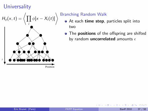
Universality
Hφ(x , t) =
⟨∏iφ[x − Xi (t)]
⟩
Position
t
Branching Random WalkAt each time step, particles split intotwoThe positions of the offspring are shiftedby random uncorrelated amounts ε
Suppose ε is uniform in [0, 1]
Hφ(x , t + 1) =
[∫ 1
0dε Hφ(x − ε, t)
]2v = 0.815172 . . . γ = 5.26208 . . .
Binary search treeDuring dt, a particle at position x is replaced with probability dt bytwo particles at position x + 1
∂tHφ(x , t) = −Hφ(x , t) + Hφ(x − 1, t)2
v = 4.31107 . . . γ = 0.768039 . . .
Éric Brunet (Paris) FKPP Equation Banff 2010 37 / 50

Universality
Hφ(x , t) =
⟨∏iφ[x − Xi (t)]
⟩
Position
t
Branching Random WalkAt each time step, particles split intotwoThe positions of the offspring are shiftedby random uncorrelated amounts εSuppose ε is uniform in [0, 1]
Hφ(x , t + 1) =
[∫ 1
0dε Hφ(x − ε, t)
]2v = 0.815172 . . . γ = 5.26208 . . .
Binary search treeDuring dt, a particle at position x is replaced with probability dt bytwo particles at position x + 1
∂tHφ(x , t) = −Hφ(x , t) + Hφ(x − 1, t)2
v = 4.31107 . . . γ = 0.768039 . . .Éric Brunet (Paris) FKPP Equation Banff 2010 37 / 50
Average distances
Hφ(x , t) =
⟨∏iφ[x − Xi (t)]
⟩
with φ =
(0
1
0
λ
)
Hφ gives the average positions of the rightmost particles
Hφ(x , t) =⟨λN(x ,t)
⟩with N(x , t) =
[Number of particles on theright of x at time t
]Hφ(x , t) = Q0(x , t) + λQ1(x , t) + λ2Q2(x , t) + · · ·
with Qn(x , t) = proba to find n particles on the right of x{∂tHφ = ∂2x Hφ − Hφ + H2
φ ∂tQ0 = ∂2x Q0 − Q0 + Q20
∂tQ1 = ∂2x Q1 − Q1 + 2Q0Q1 ∂tQ2 = ∂2x Q2 − Q2 + 2Q0Q2 + Q21
Then ∂xQn(x , t) = pn+1(x , t)− pn(x , t)
with pn(x , t) = proba to find the nth rightmost particle at x
Éric Brunet (Paris) FKPP Equation Banff 2010 38 / 50

Average distances
Hφ(x , t) =
⟨∏iφ[x − Xi (t)]
⟩with φ =
(0
1
0
λ
)
Hφ gives the average positions of the rightmost particles
Hφ(x , t) =⟨λN(x ,t)
⟩with N(x , t) =
[Number of particles on theright of x at time t
]Hφ(x , t) = Q0(x , t) + λQ1(x , t) + λ2Q2(x , t) + · · ·
with Qn(x , t) = proba to find n particles on the right of x{∂tHφ = ∂2x Hφ − Hφ + H2
φ ∂tQ0 = ∂2x Q0 − Q0 + Q20
∂tQ1 = ∂2x Q1 − Q1 + 2Q0Q1 ∂tQ2 = ∂2x Q2 − Q2 + 2Q0Q2 + Q21
Then ∂xQn(x , t) = pn+1(x , t)− pn(x , t)
with pn(x , t) = proba to find the nth rightmost particle at x
Éric Brunet (Paris) FKPP Equation Banff 2010 38 / 50
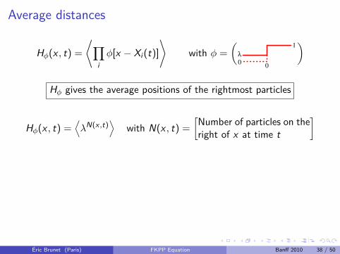
Average distances
Hφ(x , t) =
⟨∏iφ[x − Xi (t)]
⟩with φ =
(0
1
0
λ
)
Hφ gives the average positions of the rightmost particles
Hφ(x , t) =⟨λN(x ,t)
⟩with N(x , t) =
[Number of particles on theright of x at time t
]
Hφ(x , t) = Q0(x , t) + λQ1(x , t) + λ2Q2(x , t) + · · ·with Qn(x , t) = proba to find n particles on the right of x{
∂tHφ = ∂2x Hφ − Hφ + H2φ ∂tQ0 = ∂2x Q0 − Q0 + Q2
0
∂tQ1 = ∂2x Q1 − Q1 + 2Q0Q1 ∂tQ2 = ∂2x Q2 − Q2 + 2Q0Q2 + Q21
Then ∂xQn(x , t) = pn+1(x , t)− pn(x , t)
with pn(x , t) = proba to find the nth rightmost particle at x
Éric Brunet (Paris) FKPP Equation Banff 2010 38 / 50
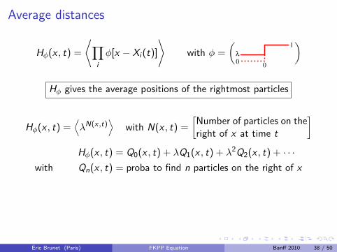
Average distances
Hφ(x , t) =
⟨∏iφ[x − Xi (t)]
⟩with φ =
(0
1
0
λ
)
Hφ gives the average positions of the rightmost particles
Hφ(x , t) =⟨λN(x ,t)
⟩with N(x , t) =
[Number of particles on theright of x at time t
]Hφ(x , t) = Q0(x , t) + λQ1(x , t) + λ2Q2(x , t) + · · ·
with Qn(x , t) = proba to find n particles on the right of x
{∂tHφ = ∂2x Hφ − Hφ + H2
φ ∂tQ0 = ∂2x Q0 − Q0 + Q20
∂tQ1 = ∂2x Q1 − Q1 + 2Q0Q1 ∂tQ2 = ∂2x Q2 − Q2 + 2Q0Q2 + Q21
Then ∂xQn(x , t) = pn+1(x , t)− pn(x , t)
with pn(x , t) = proba to find the nth rightmost particle at x
Éric Brunet (Paris) FKPP Equation Banff 2010 38 / 50

Average distances
Hφ(x , t) =
⟨∏iφ[x − Xi (t)]
⟩with φ =
(0
1
0
λ
)
Hφ gives the average positions of the rightmost particles
Hφ(x , t) =⟨λN(x ,t)
⟩with N(x , t) =
[Number of particles on theright of x at time t
]Hφ(x , t) = Q0(x , t) + λQ1(x , t) + λ2Q2(x , t) + · · ·
with Qn(x , t) = proba to find n particles on the right of x{∂tHφ = ∂2x Hφ − Hφ + H2
φ ∂tQ0 = ∂2x Q0 − Q0 + Q20
∂tQ1 = ∂2x Q1 − Q1 + 2Q0Q1 ∂tQ2 = ∂2x Q2 − Q2 + 2Q0Q2 + Q21
Then ∂xQn(x , t) = pn+1(x , t)− pn(x , t)
with pn(x , t) = proba to find the nth rightmost particle at x
Éric Brunet (Paris) FKPP Equation Banff 2010 38 / 50
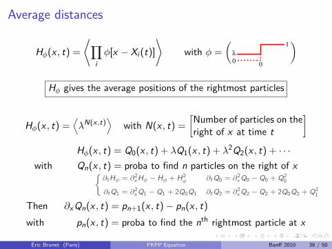
Average distances
Hφ(x , t) =
⟨∏iφ[x − Xi (t)]
⟩with φ =
(0
1
0
λ
)
Hφ gives the average positions of the rightmost particles
Hφ(x , t) =⟨λN(x ,t)
⟩with N(x , t) =
[Number of particles on theright of x at time t
]Hφ(x , t) = Q0(x , t) + λQ1(x , t) + λ2Q2(x , t) + · · ·
with Qn(x , t) = proba to find n particles on the right of x{∂tHφ = ∂2x Hφ − Hφ + H2
φ ∂tQ0 = ∂2x Q0 − Q0 + Q20
∂tQ1 = ∂2x Q1 − Q1 + 2Q0Q1 ∂tQ2 = ∂2x Q2 − Q2 + 2Q0Q2 + Q21
Then ∂xQn(x , t) = pn+1(x , t)− pn(x , t)
with pn(x , t) = proba to find the nth rightmost particle at x
Éric Brunet (Paris) FKPP Equation Banff 2010 38 / 50
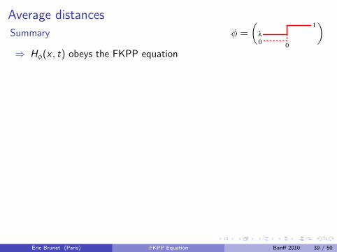
Average distancesSummary φ =
(0
1
0
λ
)⇒ Hφ(x , t) obeys the FKPP equation
⇒ deduce the equations on Qn(x , t) (proba n particles on the right of x)⇒ compute pn(x , t) (proba nth rightmost particle at x)⇒ compute 〈Xn(t)〉 (average position of nth particle)⇒ compute 〈dn,n+1(t)〉 (average distance between nth and (n + 1)th particles)
Measure the average distances by integrating p.d.e.Possible to reach large times (t ≈ 3000), no statistical noise∑
n≥1λn〈dn,n+1(t)〉 =
∫dx x∂x [Q0(x , t)− Hφ(x , t)] = Xt − Xt
Xt = 2t − 32 ln t + a0 − 3√π√
t + a1t +
a3/2t3/2 + · · ·
∑n≥1
λn〈dn,n+1(t)〉 = δ[φ] +A1t +
A3/2t3/2 + · · ·
Éric Brunet (Paris) FKPP Equation Banff 2010 39 / 50
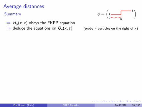
Average distancesSummary φ =
(0
1
0
λ
)⇒ Hφ(x , t) obeys the FKPP equation⇒ deduce the equations on Qn(x , t) (proba n particles on the right of x)
⇒ compute pn(x , t) (proba nth rightmost particle at x)⇒ compute 〈Xn(t)〉 (average position of nth particle)⇒ compute 〈dn,n+1(t)〉 (average distance between nth and (n + 1)th particles)
Measure the average distances by integrating p.d.e.Possible to reach large times (t ≈ 3000), no statistical noise∑
n≥1λn〈dn,n+1(t)〉 =
∫dx x∂x [Q0(x , t)− Hφ(x , t)] = Xt − Xt
Xt = 2t − 32 ln t + a0 − 3√π√
t + a1t +
a3/2t3/2 + · · ·
∑n≥1
λn〈dn,n+1(t)〉 = δ[φ] +A1t +
A3/2t3/2 + · · ·
Éric Brunet (Paris) FKPP Equation Banff 2010 39 / 50
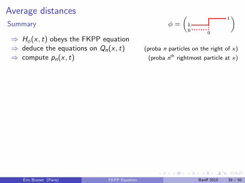
Average distancesSummary φ =
(0
1
0
λ
)⇒ Hφ(x , t) obeys the FKPP equation⇒ deduce the equations on Qn(x , t) (proba n particles on the right of x)⇒ compute pn(x , t) (proba nth rightmost particle at x)
⇒ compute 〈Xn(t)〉 (average position of nth particle)⇒ compute 〈dn,n+1(t)〉 (average distance between nth and (n + 1)th particles)
Measure the average distances by integrating p.d.e.Possible to reach large times (t ≈ 3000), no statistical noise∑
n≥1λn〈dn,n+1(t)〉 =
∫dx x∂x [Q0(x , t)− Hφ(x , t)] = Xt − Xt
Xt = 2t − 32 ln t + a0 − 3√π√
t + a1t +
a3/2t3/2 + · · ·
∑n≥1
λn〈dn,n+1(t)〉 = δ[φ] +A1t +
A3/2t3/2 + · · ·
Éric Brunet (Paris) FKPP Equation Banff 2010 39 / 50
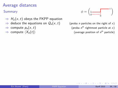
Average distancesSummary φ =
(0
1
0
λ
)⇒ Hφ(x , t) obeys the FKPP equation⇒ deduce the equations on Qn(x , t) (proba n particles on the right of x)⇒ compute pn(x , t) (proba nth rightmost particle at x)⇒ compute 〈Xn(t)〉 (average position of nth particle)
⇒ compute 〈dn,n+1(t)〉 (average distance between nth and (n + 1)th particles)
Measure the average distances by integrating p.d.e.Possible to reach large times (t ≈ 3000), no statistical noise∑
n≥1λn〈dn,n+1(t)〉 =
∫dx x∂x [Q0(x , t)− Hφ(x , t)] = Xt − Xt
Xt = 2t − 32 ln t + a0 − 3√π√
t + a1t +
a3/2t3/2 + · · ·
∑n≥1
λn〈dn,n+1(t)〉 = δ[φ] +A1t +
A3/2t3/2 + · · ·
Éric Brunet (Paris) FKPP Equation Banff 2010 39 / 50
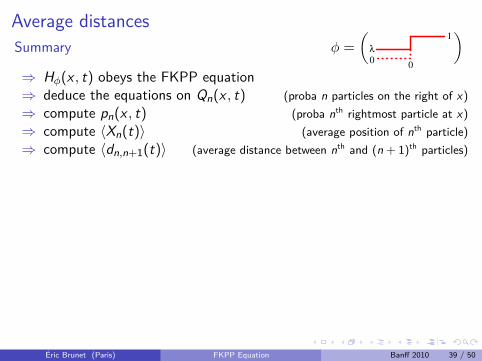
Average distancesSummary φ =
(0
1
0
λ
)⇒ Hφ(x , t) obeys the FKPP equation⇒ deduce the equations on Qn(x , t) (proba n particles on the right of x)⇒ compute pn(x , t) (proba nth rightmost particle at x)⇒ compute 〈Xn(t)〉 (average position of nth particle)⇒ compute 〈dn,n+1(t)〉 (average distance between nth and (n + 1)th particles)
Measure the average distances by integrating p.d.e.Possible to reach large times (t ≈ 3000), no statistical noise∑
n≥1λn〈dn,n+1(t)〉 =
∫dx x∂x [Q0(x , t)− Hφ(x , t)] = Xt − Xt
Xt = 2t − 32 ln t + a0 − 3√π√
t + a1t +
a3/2t3/2 + · · ·
∑n≥1
λn〈dn,n+1(t)〉 = δ[φ] +A1t +
A3/2t3/2 + · · ·
Éric Brunet (Paris) FKPP Equation Banff 2010 39 / 50
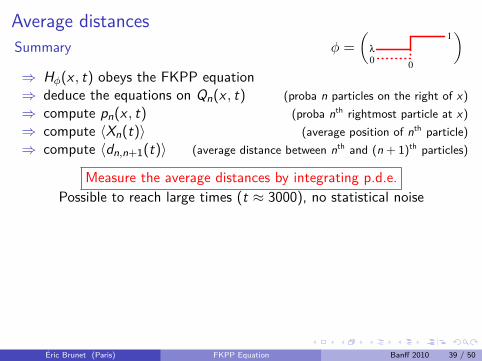
Average distancesSummary φ =
(0
1
0
λ
)⇒ Hφ(x , t) obeys the FKPP equation⇒ deduce the equations on Qn(x , t) (proba n particles on the right of x)⇒ compute pn(x , t) (proba nth rightmost particle at x)⇒ compute 〈Xn(t)〉 (average position of nth particle)⇒ compute 〈dn,n+1(t)〉 (average distance between nth and (n + 1)th particles)
Measure the average distances by integrating p.d.e.Possible to reach large times (t ≈ 3000), no statistical noise
∑n≥1
λn〈dn,n+1(t)〉 =
∫dx x∂x [Q0(x , t)− Hφ(x , t)] = Xt − Xt
Xt = 2t − 32 ln t + a0 − 3√π√
t + a1t +
a3/2t3/2 + · · ·
∑n≥1
λn〈dn,n+1(t)〉 = δ[φ] +A1t +
A3/2t3/2 + · · ·
Éric Brunet (Paris) FKPP Equation Banff 2010 39 / 50
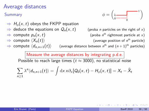
Average distancesSummary φ =
(0
1
0
λ
)⇒ Hφ(x , t) obeys the FKPP equation⇒ deduce the equations on Qn(x , t) (proba n particles on the right of x)⇒ compute pn(x , t) (proba nth rightmost particle at x)⇒ compute 〈Xn(t)〉 (average position of nth particle)⇒ compute 〈dn,n+1(t)〉 (average distance between nth and (n + 1)th particles)
Measure the average distances by integrating p.d.e.Possible to reach large times (t ≈ 3000), no statistical noise∑
n≥1λn〈dn,n+1(t)〉 =
∫dx x∂x [Q0(x , t)− Hφ(x , t)] = Xt − Xt
Xt = 2t − 32 ln t + a0 − 3√π√
t + a1t +
a3/2t3/2 + · · ·
∑n≥1
λn〈dn,n+1(t)〉 = δ[φ] +A1t +
A3/2t3/2 + · · ·
Éric Brunet (Paris) FKPP Equation Banff 2010 39 / 50
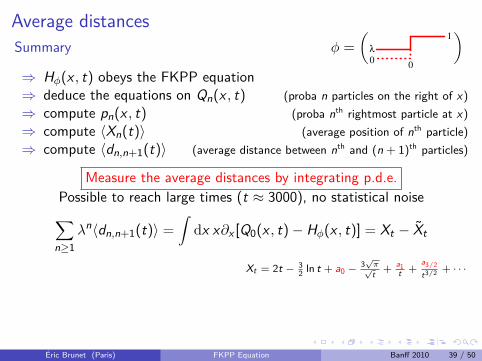
Average distancesSummary φ =
(0
1
0
λ
)⇒ Hφ(x , t) obeys the FKPP equation⇒ deduce the equations on Qn(x , t) (proba n particles on the right of x)⇒ compute pn(x , t) (proba nth rightmost particle at x)⇒ compute 〈Xn(t)〉 (average position of nth particle)⇒ compute 〈dn,n+1(t)〉 (average distance between nth and (n + 1)th particles)
Measure the average distances by integrating p.d.e.Possible to reach large times (t ≈ 3000), no statistical noise∑
n≥1λn〈dn,n+1(t)〉 =
∫dx x∂x [Q0(x , t)− Hφ(x , t)] = Xt − Xt
Xt = 2t − 32 ln t + a0 − 3√π√
t + a1t +
a3/2t3/2 + · · ·
∑n≥1
λn〈dn,n+1(t)〉 = δ[φ] +A1t +
A3/2t3/2 + · · ·
Éric Brunet (Paris) FKPP Equation Banff 2010 39 / 50
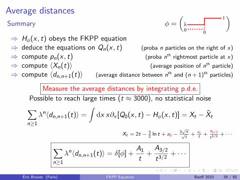
Average distancesSummary φ =
(0
1
0
λ
)⇒ Hφ(x , t) obeys the FKPP equation⇒ deduce the equations on Qn(x , t) (proba n particles on the right of x)⇒ compute pn(x , t) (proba nth rightmost particle at x)⇒ compute 〈Xn(t)〉 (average position of nth particle)⇒ compute 〈dn,n+1(t)〉 (average distance between nth and (n + 1)th particles)
Measure the average distances by integrating p.d.e.Possible to reach large times (t ≈ 3000), no statistical noise∑
n≥1λn〈dn,n+1(t)〉 =
∫dx x∂x [Q0(x , t)− Hφ(x , t)] = Xt − Xt
Xt = 2t − 32 ln t + a0 − 3√π√
t + a1t +
a3/2t3/2 + · · ·
∑n≥1
λn〈dn,n+1(t)〉 = δ[φ] +A1t +
A3/2t3/2 + · · ·
Éric Brunet (Paris) FKPP Equation Banff 2010 39 / 50

Numerical results: average distancesThe results: average distances as a function of 1/t
⟨d3,4⟩
150
165
1100
1200
0
0.224
0.223
0.222
0.221
0.220
0.219
⟨d2,3⟩
150
165
1100
1200
0
0.309
0.308
0.307
0.306
0.305
0.304
0.303
⟨d1,2⟩
150
165
1100
1200
0
0.503
0.502
0.501
0.500
0.499
0.498
0.497
0.496
In the long time limit
〈d1,2〉st ' 0.496 〈d2,3〉st ' 0.303 〈d3,4〉st ' 0.219〈d4,5〉st ' 0.172 〈d5,6〉st ' 0.142 〈d6,7〉st ' 0.121
Éric Brunet (Paris) FKPP Equation Banff 2010 40 / 50
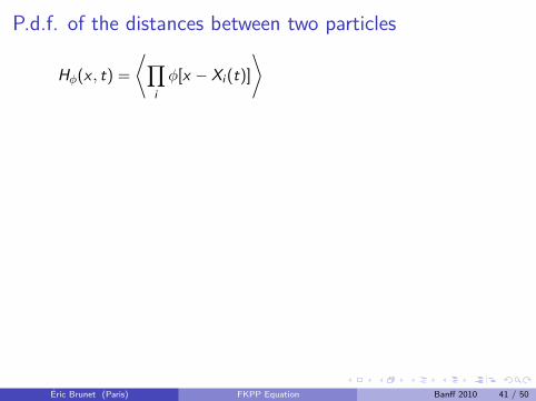
P.d.f. of the distances between two particles
Hφ(x , t) =
⟨∏iφ[x − Xi (t)]
⟩
with φ =
(1
0
λµ0
λ
−a
)
Hφ(x , t) =⟨λN(x ,t)µN(x+a,t)
⟩with N(x , t) =
[Number of particles on theright of x at time t
]
⇒ Qmn(x , a, t) = Proba[N(x , t) = n and N(x + a, t) = m
]⇒ Rmn(x , a, t) = Proba
[N(x , t) < n and N(x + a, t) < m
]⇒ (∂x−∂a)Rmn(x , a, t)dx = Proba
[Xn(t) ∈ dx and N(x +a, t) < m
]⇒ (∂x − ∂a)Rmn(x , a, t)dx = Proba
[Xn(t) ∈ dx and Xm(t) < x + a
]⇒
∫dx (∂x − ∂a)Rmn(x , a, t) = Proba
[Xm(t)− Xn(t) < a
]Hφ gives the p.d.f. of the distance between mth and nth particles
Éric Brunet (Paris) FKPP Equation Banff 2010 41 / 50
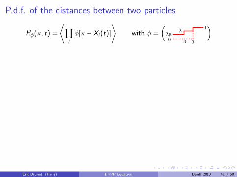
P.d.f. of the distances between two particles
Hφ(x , t) =
⟨∏iφ[x − Xi (t)]
⟩with φ =
(1
0
λµ0
λ
−a
)
Hφ(x , t) =⟨λN(x ,t)µN(x+a,t)
⟩with N(x , t) =
[Number of particles on theright of x at time t
]
⇒ Qmn(x , a, t) = Proba[N(x , t) = n and N(x + a, t) = m
]⇒ Rmn(x , a, t) = Proba
[N(x , t) < n and N(x + a, t) < m
]⇒ (∂x−∂a)Rmn(x , a, t)dx = Proba
[Xn(t) ∈ dx and N(x +a, t) < m
]⇒ (∂x − ∂a)Rmn(x , a, t)dx = Proba
[Xn(t) ∈ dx and Xm(t) < x + a
]⇒
∫dx (∂x − ∂a)Rmn(x , a, t) = Proba
[Xm(t)− Xn(t) < a
]Hφ gives the p.d.f. of the distance between mth and nth particles
Éric Brunet (Paris) FKPP Equation Banff 2010 41 / 50
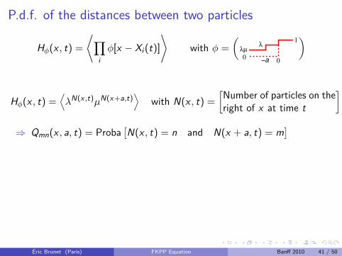
P.d.f. of the distances between two particles
Hφ(x , t) =
⟨∏iφ[x − Xi (t)]
⟩with φ =
(1
0
λµ0
λ
−a
)
Hφ(x , t) =⟨λN(x ,t)µN(x+a,t)
⟩with N(x , t) =
[Number of particles on theright of x at time t
]
⇒ Qmn(x , a, t) = Proba[N(x , t) = n and N(x + a, t) = m
]
⇒ Rmn(x , a, t) = Proba[N(x , t) < n and N(x + a, t) < m
]⇒ (∂x−∂a)Rmn(x , a, t)dx = Proba
[Xn(t) ∈ dx and N(x +a, t) < m
]⇒ (∂x − ∂a)Rmn(x , a, t)dx = Proba
[Xn(t) ∈ dx and Xm(t) < x + a
]⇒
∫dx (∂x − ∂a)Rmn(x , a, t) = Proba
[Xm(t)− Xn(t) < a
]Hφ gives the p.d.f. of the distance between mth and nth particles
Éric Brunet (Paris) FKPP Equation Banff 2010 41 / 50

P.d.f. of the distances between two particles
Hφ(x , t) =
⟨∏iφ[x − Xi (t)]
⟩with φ =
(1
0
λµ0
λ
−a
)
Hφ(x , t) =⟨λN(x ,t)µN(x+a,t)
⟩with N(x , t) =
[Number of particles on theright of x at time t
]
⇒ Qmn(x , a, t) = Proba[N(x , t) = n and N(x + a, t) = m
]⇒ Rmn(x , a, t) = Proba
[N(x , t) < n and N(x + a, t) < m
]
⇒ (∂x−∂a)Rmn(x , a, t)dx = Proba[Xn(t) ∈ dx and N(x +a, t) < m
]⇒ (∂x − ∂a)Rmn(x , a, t)dx = Proba
[Xn(t) ∈ dx and Xm(t) < x + a
]⇒
∫dx (∂x − ∂a)Rmn(x , a, t) = Proba
[Xm(t)− Xn(t) < a
]Hφ gives the p.d.f. of the distance between mth and nth particles
Éric Brunet (Paris) FKPP Equation Banff 2010 41 / 50
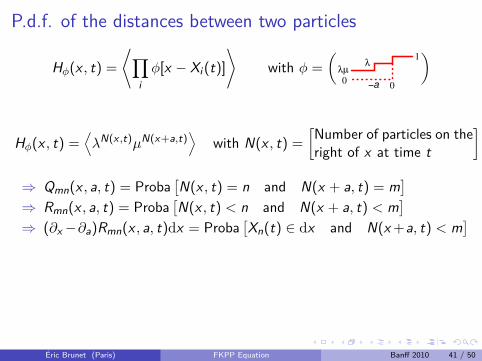
P.d.f. of the distances between two particles
Hφ(x , t) =
⟨∏iφ[x − Xi (t)]
⟩with φ =
(1
0
λµ0
λ
−a
)
Hφ(x , t) =⟨λN(x ,t)µN(x+a,t)
⟩with N(x , t) =
[Number of particles on theright of x at time t
]
⇒ Qmn(x , a, t) = Proba[N(x , t) = n and N(x + a, t) = m
]⇒ Rmn(x , a, t) = Proba
[N(x , t) < n and N(x + a, t) < m
]⇒ (∂x−∂a)Rmn(x , a, t)dx = Proba
[Xn(t) ∈ dx and N(x +a, t) < m
]
⇒ (∂x − ∂a)Rmn(x , a, t)dx = Proba[Xn(t) ∈ dx and Xm(t) < x + a
]⇒
∫dx (∂x − ∂a)Rmn(x , a, t) = Proba
[Xm(t)− Xn(t) < a
]Hφ gives the p.d.f. of the distance between mth and nth particles
Éric Brunet (Paris) FKPP Equation Banff 2010 41 / 50
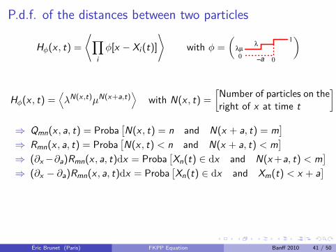
P.d.f. of the distances between two particles
Hφ(x , t) =
⟨∏iφ[x − Xi (t)]
⟩with φ =
(1
0
λµ0
λ
−a
)
Hφ(x , t) =⟨λN(x ,t)µN(x+a,t)
⟩with N(x , t) =
[Number of particles on theright of x at time t
]
⇒ Qmn(x , a, t) = Proba[N(x , t) = n and N(x + a, t) = m
]⇒ Rmn(x , a, t) = Proba
[N(x , t) < n and N(x + a, t) < m
]⇒ (∂x−∂a)Rmn(x , a, t)dx = Proba
[Xn(t) ∈ dx and N(x +a, t) < m
]⇒ (∂x − ∂a)Rmn(x , a, t)dx = Proba
[Xn(t) ∈ dx and Xm(t) < x + a
]
⇒∫
dx (∂x − ∂a)Rmn(x , a, t) = Proba[Xm(t)− Xn(t) < a
]Hφ gives the p.d.f. of the distance between mth and nth particles
Éric Brunet (Paris) FKPP Equation Banff 2010 41 / 50
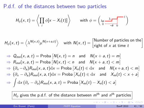
P.d.f. of the distances between two particles
Hφ(x , t) =
⟨∏iφ[x − Xi (t)]
⟩with φ =
(1
0
λµ0
λ
−a
)
Hφ(x , t) =⟨λN(x ,t)µN(x+a,t)
⟩with N(x , t) =
[Number of particles on theright of x at time t
]
⇒ Qmn(x , a, t) = Proba[N(x , t) = n and N(x + a, t) = m
]⇒ Rmn(x , a, t) = Proba
[N(x , t) < n and N(x + a, t) < m
]⇒ (∂x−∂a)Rmn(x , a, t)dx = Proba
[Xn(t) ∈ dx and N(x +a, t) < m
]⇒ (∂x − ∂a)Rmn(x , a, t)dx = Proba
[Xn(t) ∈ dx and Xm(t) < x + a
]⇒
∫dx (∂x − ∂a)Rmn(x , a, t) = Proba
[Xm(t)− Xn(t) < a
]Hφ gives the p.d.f. of the distance between mth and nth particles
Éric Brunet (Paris) FKPP Equation Banff 2010 41 / 50

Numerical results: p.d.f. of the distances
As of function of a, density of probability that X1 − X2 = a
2e−2adatapoints
32.521.510.50
2.01.81.61.41.21.00.80.60.40.20.0
e−(1+√
2)a2e−2a
datapoints110−50
10−100
10−150
10−200
10−250
10−300
10−350
10−400
4003002001000
Éric Brunet (Paris) FKPP Equation Banff 2010 42 / 50
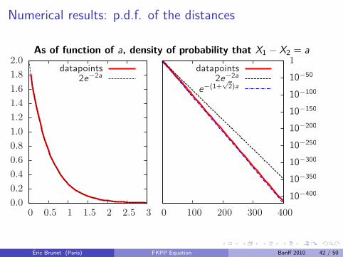

Density at a distance a
Hφ(x , t) =
⟨∏iφ[x − Xi (t)]
⟩
with φ =
(1
0
−λe
0 a
)
Hφ(x , t) =⟨e−λN(x−a,t)
1N(x ,t)=0⟩
⇒ (∂x + ∂a)Hφ(x , t)dx =⟨e−λN(x−a,t)
1X1(t)∈dx⟩
⇒ 1 +
∫dx ∂aHφ(x , t) =
⟨e−λN(X1(t)−a,t)
⟩Hφ gives the generating function of the number ofparticles within a distance a of the rightmost particle
Éric Brunet (Paris) FKPP Equation Banff 2010 43 / 50
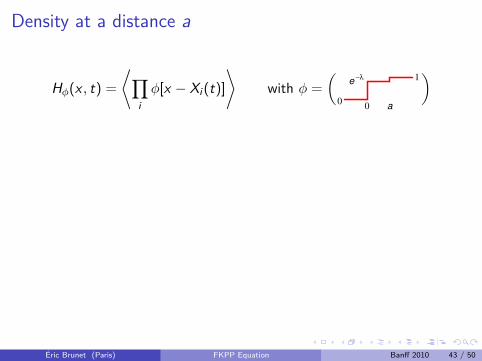
Density at a distance a
Hφ(x , t) =
⟨∏iφ[x − Xi (t)]
⟩with φ =
(1
0
−λe
0 a
)
Hφ(x , t) =⟨e−λN(x−a,t)
1N(x ,t)=0⟩
⇒ (∂x + ∂a)Hφ(x , t)dx =⟨e−λN(x−a,t)
1X1(t)∈dx⟩
⇒ 1 +
∫dx ∂aHφ(x , t) =
⟨e−λN(X1(t)−a,t)
⟩Hφ gives the generating function of the number ofparticles within a distance a of the rightmost particle
Éric Brunet (Paris) FKPP Equation Banff 2010 43 / 50
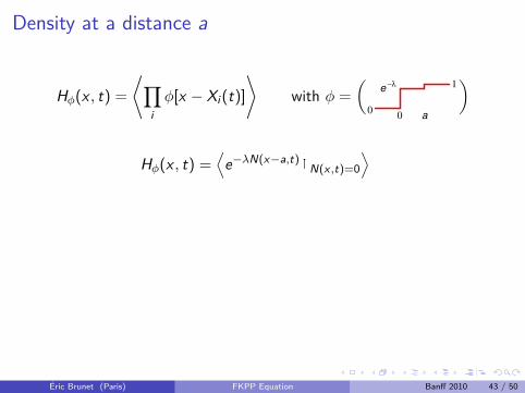
Density at a distance a
Hφ(x , t) =
⟨∏iφ[x − Xi (t)]
⟩with φ =
(1
0
−λe
0 a
)
Hφ(x , t) =⟨e−λN(x−a,t)
1N(x ,t)=0⟩
⇒ (∂x + ∂a)Hφ(x , t)dx =⟨e−λN(x−a,t)
1X1(t)∈dx⟩
⇒ 1 +
∫dx ∂aHφ(x , t) =
⟨e−λN(X1(t)−a,t)
⟩Hφ gives the generating function of the number ofparticles within a distance a of the rightmost particle
Éric Brunet (Paris) FKPP Equation Banff 2010 43 / 50
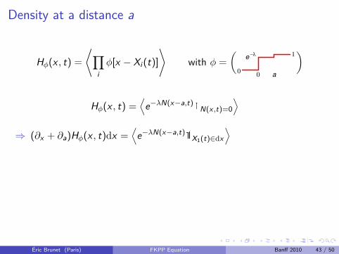
Density at a distance a
Hφ(x , t) =
⟨∏iφ[x − Xi (t)]
⟩with φ =
(1
0
−λe
0 a
)
Hφ(x , t) =⟨e−λN(x−a,t)
1N(x ,t)=0⟩
⇒ (∂x + ∂a)Hφ(x , t)dx =⟨e−λN(x−a,t)
1X1(t)∈dx⟩
⇒ 1 +
∫dx ∂aHφ(x , t) =
⟨e−λN(X1(t)−a,t)
⟩Hφ gives the generating function of the number ofparticles within a distance a of the rightmost particle
Éric Brunet (Paris) FKPP Equation Banff 2010 43 / 50
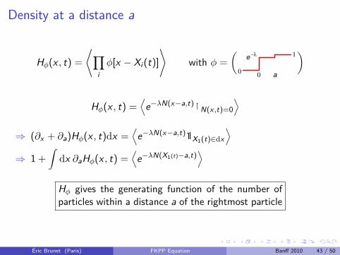
Density at a distance a
Hφ(x , t) =
⟨∏iφ[x − Xi (t)]
⟩with φ =
(1
0
−λe
0 a
)
Hφ(x , t) =⟨e−λN(x−a,t)
1N(x ,t)=0⟩
⇒ (∂x + ∂a)Hφ(x , t)dx =⟨e−λN(x−a,t)
1X1(t)∈dx⟩
⇒ 1 +
∫dx ∂aHφ(x , t) =
⟨e−λN(X1(t)−a,t)
⟩Hφ gives the generating function of the number ofparticles within a distance a of the rightmost particle
Éric Brunet (Paris) FKPP Equation Banff 2010 43 / 50

Numerical results: density at a distance aρ1(X1 − a)e−a as a function of a
302520151050
2018161412108642
ρ1(X1 − a) =1da
(Average number of particles in an interval daat a distance a of the rightmost particle
)
ρ1(X1 − a) ' aea
Éric Brunet (Paris) FKPP Equation Banff 2010 44 / 50

Numerical results: density at a distance aρ1(X1 − a)e−a as a function of a
302520151050
2018161412108642
ρ1(X1 − a) =1da
(Average number of particles in an interval daat a distance a of the rightmost particle
)
ρ1(X1 − a) ' aea
Éric Brunet (Paris) FKPP Equation Banff 2010 44 / 50
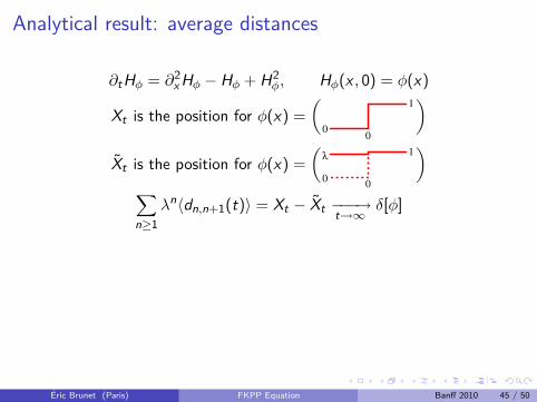
Analytical result: average distances
∂tHφ = ∂2x Hφ − Hφ + H2φ, Hφ(x , 0) = φ(x)
Xt is the position for φ(x) =
(0
0
1)
Xt is the position for φ(x) =
(0
1
0
λ
)∑n≥1
λn〈dn,n+1(t)〉 = Xt − Xt −−−→t→∞δ[φ]
For λ close to 1, δ[φ] = τλ − ln τλ +O(1) with τλ = − ln(1− λ)
〈dn,n+1〉st =1n −
1n ln n + · · · for large n
Éric Brunet (Paris) FKPP Equation Banff 2010 45 / 50
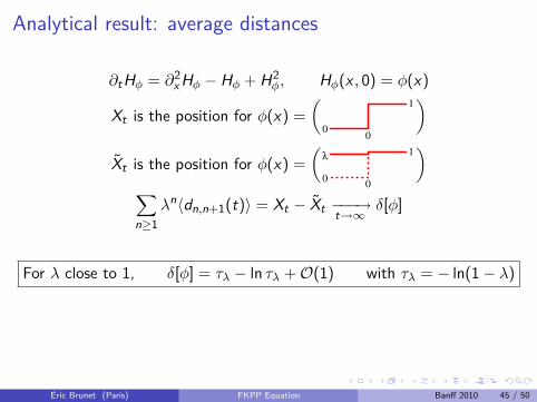
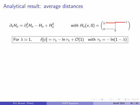
Analytical result: average distances
∂tHφ = ∂2x Hφ − Hφ + H2φ with Hφ(x , 0) =
(0
1
0
λ
)
For λ ' 1, δ[φ] = τλ − ln τλ +O(1) with τλ = − ln(1− λ)
τλ = time needed for Hφ(−∞, 0) to “reach” 0As long as t � τλ, one has 1− Hφ � 1
1− Hφ(x , t) ' 1− λ2 et erfc
( x√4t
)for t � τλ or x large enough
Xt is the position, let vt = ∂tXt be the velocity. For t large enough,Hφ(x , t) ' Fvt (x − Xt)
' 1− A1(vt)e−γt (x−Xt )
Matching in the range 1� x − Xt �√
t gives the resultAs a bonus: Xt ≈ 2t
√1− τλ/t.
Éric Brunet (Paris) FKPP Equation Banff 2010 46 / 50

Analytical result: average distances
∂tHφ = ∂2x Hφ − Hφ + H2φ with Hφ(x , 0) =
(0
1
0
λ
)
For λ ' 1, δ[φ] = τλ − ln τλ +O(1) with τλ = − ln(1− λ)
τλ = time needed for Hφ(−∞, 0) to “reach” 0As long as t � τλ, one has 1− Hφ � 1
1− Hφ(x , t) ' 1− λ2 et erfc
( x√4t
)for t � τλ
or x large enough
Xt is the position, let vt = ∂tXt be the velocity. For t large enough,Hφ(x , t) ' Fvt (x − Xt)
' 1− A1(vt)e−γt (x−Xt )
Matching in the range 1� x − Xt �√
t gives the resultAs a bonus: Xt ≈ 2t
√1− τλ/t.
Éric Brunet (Paris) FKPP Equation Banff 2010 46 / 50

Analytical result: average distances
∂tHφ = ∂2x Hφ − Hφ + H2φ with Hφ(x , 0) =
(0
1
0
λ
)
For λ ' 1, δ[φ] = τλ − ln τλ +O(1) with τλ = − ln(1− λ)
τλ = time needed for Hφ(−∞, 0) to “reach” 0As long as t � τλ, one has 1− Hφ � 1
1− Hφ(x , t) ' 1− λ2 et erfc
( x√4t
)for t � τλ or x large enough
Xt is the position, let vt = ∂tXt be the velocity. For t large enough,Hφ(x , t) ' Fvt (x − Xt)
' 1− A1(vt)e−γt (x−Xt )
Matching in the range 1� x − Xt �√
t gives the resultAs a bonus: Xt ≈ 2t
√1− τλ/t.
Éric Brunet (Paris) FKPP Equation Banff 2010 46 / 50
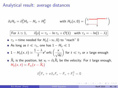
Analytical result: average distances
∂tHφ = ∂2x Hφ − Hφ + H2φ with Hφ(x , 0) =
(0
1
0
λ
)
For λ ' 1, δ[φ] = τλ − ln τλ +O(1) with τλ = − ln(1− λ)
τλ = time needed for Hφ(−∞, 0) to “reach” 0As long as t � τλ, one has 1− Hφ � 1
1− Hφ(x , t) ' 1− λ2 et erfc
( x√4t
)for t � τλ or x large enough
Xt is the position, let vt = ∂tXt be the velocity. For t large enough,Hφ(x , t) ' Fvt (x − Xt)
' 1− A1(vt)e−γt (x−Xt )
Matching in the range 1� x − Xt �√
t gives the resultAs a bonus: Xt ≈ 2t
√1− τλ/t.
∂2x Fv + v∂xFv − Fv + F 2v = 0
Éric Brunet (Paris) FKPP Equation Banff 2010 46 / 50
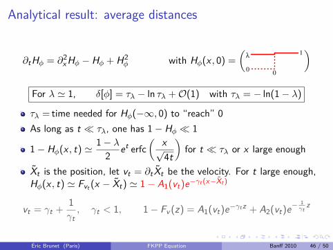
Analytical result: average distances
∂tHφ = ∂2x Hφ − Hφ + H2φ with Hφ(x , 0) =
(0
1
0
λ
)
For λ ' 1, δ[φ] = τλ − ln τλ +O(1) with τλ = − ln(1− λ)
τλ = time needed for Hφ(−∞, 0) to “reach” 0As long as t � τλ, one has 1− Hφ � 1
1− Hφ(x , t) ' 1− λ2 et erfc
( x√4t
)for t � τλ or x large enough
Xt is the position, let vt = ∂tXt be the velocity. For t large enough,Hφ(x , t) ' Fvt (x − Xt) ' 1− A1(vt)e−γt (x−Xt )
Matching in the range 1� x − Xt �√
t gives the resultAs a bonus: Xt ≈ 2t
√1− τλ/t.
vt = γt +1γt, γt < 1, 1− Fv (z) = A1(vt)e−γtz + A2(vt)e−
1γt
z
Éric Brunet (Paris) FKPP Equation Banff 2010 46 / 50
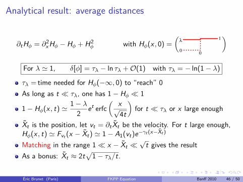
Analytical result: average distances
∂tHφ = ∂2x Hφ − Hφ + H2φ with Hφ(x , 0) =
(0
1
0
λ
)
For λ ' 1, δ[φ] = τλ − ln τλ +O(1) with τλ = − ln(1− λ)
τλ = time needed for Hφ(−∞, 0) to “reach” 0As long as t � τλ, one has 1− Hφ � 1
1− Hφ(x , t) ' 1− λ2 et erfc
( x√4t
)for t � τλ or x large enough
Xt is the position, let vt = ∂tXt be the velocity. For t large enough,Hφ(x , t) ' Fvt (x − Xt) ' 1− A1(vt)e−γt (x−Xt )
Matching in the range 1� x − Xt �√
t gives the resultAs a bonus: Xt ≈ 2t
√1− τλ/t.
Éric Brunet (Paris) FKPP Equation Banff 2010 46 / 50
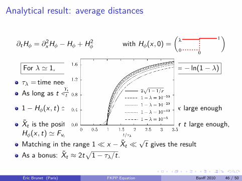
Analytical result: average distances
∂tHφ = ∂2x Hφ − Hφ + H2φ with Hφ(x , 0) =
(0
1
0
λ
)
For λ ' 1, δ[φ] = τλ − ln τλ +O(1) with τλ = − ln(1− λ)
τλ = time needed for Hφ(−∞, 0) to “reach” 0As long as t � τλ, one has 1− Hφ � 1
1− Hφ(x , t) ' 1− λ2 et erfc
( x√4t
)for t � τλ or x large enough
Xt is the position, let vt = ∂tXt be the velocity. For t large enough,Hφ(x , t) ' Fvt (x − Xt) ' 1− A1(vt)e−γt (x−Xt )
Matching in the range 1� x − Xt �√
t gives the resultAs a bonus: Xt ≈ 2t
√1− τλ/t.
Éric Brunet (Paris) FKPP Equation Banff 2010 46 / 50

Analytical result: distance and densityP.d.f. of the distances:φ =
(1
0
λµ0
λ
−a
)=⇒ Qmn(x , a, t) =⇒ Rmn(x , a, t) =⇒ . . .
Number of particles on the right of X1(t)− a: φ =(
1
0
−λe
0 a
)=⇒ . . .
∂tQ = ∂2x Q − Q + Q2 with Q(x , 0) =(
00
1)
∂tRa = ∂2x Ra − Ra + 2QRa with Ra(x , 0) = δ(x + a) =(
0−a 0
1)
∂t Ra = ∂2x Ra − Ra + 2QRa with Ra(x , 0) = δ(x − a) =(
00
1
a
)
Proba[X1(t)− X2(t) > a] =
∫dx Ra(x , t)
≈ e−(1+√2)a ?
⟨N(X1(t)− a, t)
⟩=
∫dx Ra(x , t)
≈ aea ?
Ra(x , t)→ λaQ′(x , t) for t large
Éric Brunet (Paris) FKPP Equation Banff 2010 47 / 50
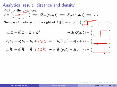

Analytical result: distance and densityP.d.f. of the distances:φ =
(1
0
λµ0
λ
−a
)=⇒ Qmn(x , a, t) =⇒ Rmn(x , a, t) =⇒ . . .
Number of particles on the right of X1(t)− a: φ =(
1
0
−λe
0 a
)=⇒ . . .
∂tQ = ∂2x Q − Q + Q2 with Q(x , 0) =(
00
1)
∂tRa = ∂2x Ra − Ra + 2QRa with Ra(x , 0) = δ(x + a) =(
0−a 0
1)
∂t Ra = ∂2x Ra − Ra + 2QRa with Ra(x , 0) = δ(x − a) =(
00
1
a
)
Proba[X1(t)− X2(t) > a] =
∫dx Ra(x , t) ≈ e−(1+
√2)a ?⟨
N(X1(t)− a, t)⟩
=
∫dx Ra(x , t) ≈ aea ?
Ra(x , t)→ λaQ′(x , t) for t largeÉric Brunet (Paris) FKPP Equation Banff 2010 47 / 50

Thank you !
Éric Brunet (Paris) FKPP Equation Banff 2010 48 / 50

Exponential model
N particles, discrete timeEach particle has infinitely many offspringgiven by a Poisson process of density ψ: foreach dx , there is an offspring with probabilityψ(x − xparent) dxOne only keep the N rightmost particles of a given generation
Usually a Fisher equation
v(γ) =1γln(∫
dε ψ(ε)eγε)
But not always: ψ(ε) = e−ε
Éric Brunet (Paris) FKPP Equation Banff 2010 49 / 50
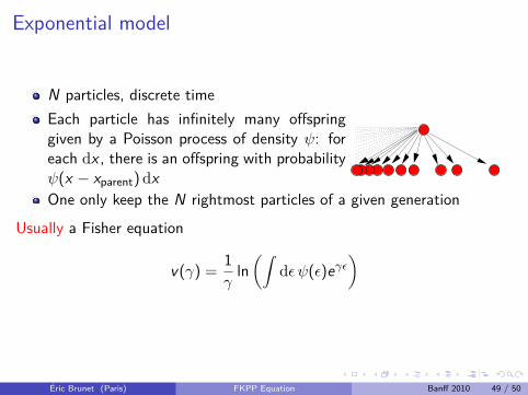

Exponential model vs FisherExponential model Fisher case
vN ln(lnN + ln lnN) +O( 1lnN
)v∗ − A
(lnN + 3 ln lnN)2
DNπ2
3(lnN + ln lnN)+O
( 1ln2 N
) B(lnN+???)3
p(δ) e−δ C1e−γ∗δ
R(δ) ln(1 +
eδlnN
)1γ∗
ln(1 + C2
eγ∗δ
ln3 N
)Relaxation time 1 ln2 N
Fluctuation size ln lnN 1γ∗
3 ln lnN
Conclusion
Éric Brunet (Paris) FKPP Equation Banff 2010 50 / 50


![Kpp book eng[1]](https://static.documents.pub/doc/80x56/5562a17fd8b42a7c4a8b47ed/kpp-book-eng1.jpg)


