Electronic copy available at: http://ssrn.com/abstract=1686004

The Flash Crash: The Impact of High FrequencyTrading on an Electronic Market∗

Andrei Kirilenko—MIT Sloan School of ManagementAlbert S. Kyle—University of Maryland

Mehrdad Samadi—University of North CarolinaTugkan Tuzun—Board of Governors of the Federal Reserve System

Original Version: October 1, 2010Revised version: September 24, 2014

ABSTRACT

We present an empirical analysis of the Flash Crash – a systemic market eventon May 6, 2010. The Flash Crash was blamed on high frequency traders (HFTs)– hyperactive trading algorithms operating inside automated markets. We useaudit-trail data for the E-mini S&P 500 futures contract to show that HFTs didnot cause the Flash Crash – a large sell program did – but exacerbated the pricemovement by absorbing immediacy ahead of others. We present novel findingson the trading behavior of HFTs as part of a market ecosystem and proposerecommendations for making automated markets more resilient to large liquidityimbalances.

∗We thank participants at numerous seminars and conferences for very helpful comments and sug-gestions. The views presented in this paper are our own and do not represent a position of any officialagency, its management or staff.

Electronic copy available at: http://ssrn.com/abstract=1686004

A draft of this paper was originally authorized for public distribution by the U.S.Commodity Futures Trading Commission (CFTC) prior to the release of the joint reportof the staffs of the CFTC and the U.S. Securities and Exchange Commission (SEC) en-titled “Findings Regarding the Market Events of May 6, 2010”. The CFTC-SEC reportwas issued to the public on September 30, 2010. Prior to the release, all matters relatedto the aggregation of data, presentation of results, and sharing the results with the pub-lic were reviewed by the CFTC Senior Staff, reviewers in the Office of the Chairman,the Division of Market Oversight, the Office of the General Counsel, the Division ofEnforcement, as well as staff from other divisions of the CFTC. CFTC Chairman andCommissioners were briefed on the analysis and results of the paper prior to the publicrelease of the report.

On February 21, 2014, after a lengthy review process, the CFTC re-authorized thispaper for public distribution and stated that the following disclaimer must be used:The research presented in this paper was co-authored by Andrei Kirilenko, a formerfull-time CFTC employee, Albert Kyle, a former CFTC contractor who performed workunder CFTC OCE contract (CFCE-09-CO-0147), Mehrdad Samadi, a former full-timeCFTC employee and former CFTC contractor who performed work under CFTC OCEcontracts (CFCE-11-CO-0122 and CFOCE-13-CO-0061), and Tugkan Tuzun, a formerCFTC contractor who performed work under CFTC OCE contract (CFCE-10-CO-0175).The Office of the Chief Economist and CFTC economists produce original research ona broad range of topics relevant to the CFTC’s mandate to regulate commodity fu-tures markets, commodity options markets, and the expanded mandate to regulate theswaps markets pursuant to the Dodd-Frank Wall Street Reform and Consumer Protec-tion Act. These papers are often presented at conferences and many of these papersare later published by peer-review and other scholarly outlets. The analyses and con-clusions expressed in this paper are those of the authors and do not reflect the viewsof other members of the Office of the Chief Economist, other Commission staff, or theCommission itself.

2

On May 6, 2010, in the course of about 36 minutes starting at 2:32pm ET, U.S.financial markets experienced one of the most turbulent periods in their history. Broadstock market indices – the S&P 500, the Nasdaq 100, and the Russell 2000, collapsedand rebounded with extraordinary velocity. The Dow Jones Industrial Average (DJIA)experienced the biggest intraday point decline in its entire history. Stock index futures,options, and exchange-traded funds, as well as individual stocks experienced extraor-dinary price volatility often accompanied by spikes in trading volume. Because thesedramatic events happened so quickly, the events of May 6, 2010, have become known asthe “Flash Crash.”

This paper uses audit trail data during May 3-6, 2010 to examine the ecosystemof the S&P 500 E-mini futures during these four days and the role of high frequencytraders and other market participants in the Flash Crash. The audit trail dataset:(i) contains time stamps for all trades up to the second; (ii) sequences trades withineach second; (iii) identifies the account numbers of the two participants for each trade;(iv) distinguishes between the buyer and a seller for each trade, and (v) distinguishesbetween the participant that originated the trade (aggressive side) and the participantwhose order was executed against (passive side).

On September 30, 2010, the staffs of the Commodity Futures Trading Commission(CFTC) and Securities and Exchange Commission (SEC) issued a report on the eventsof May 6, 2010. The 104-page report described how an automated execution programto sell 75,000 contracts of the E-Mini S&P 500 futures, algorithmic trading activity, andobscure order submission practices all conspired to create the Flash Crash.1

In the aftermath of the Flash Crash, the media became particularly fascinated withthe secretive blend of high-powered technology and hyperactive market activity knownas high frequency trading (HFT).2 To many investors and market commentators, highfrequency trading has become the root cause of the unfairness and fragility of automatedmarkets.3 In response to public pressure, government regulators and self-regulatoryorganizations (e.g., securities and derivatives exchanges) around the world have comeup with a variety of anti-HFT measures. These measures range from a tax on financial

1The CFTC-SEC report’s narrative of the triggering event of the Flash Crash was based in part onthe preliminary analysis contained in the original version of this paper (see footnote 22 of the CFTC-SEC report). The narrative (the report) and the analysis (the paper) were presented separately inpart because the CFTC-SEC report was written for a very broad audience, while the methodologyand preliminary results in the original paper were intended for peer review by research scientists andmarket experts. Both the report and the paper serve the same purpose of describing to the marketparticipants, the research community, and the general public how unrelated trading algorithms activatedacross different parts of the financial marketplace can cascade into a systemic event for the entire U.Sfinancial market. The original version of this paper has been cited by numerous academic, government-sponsored and industry-sponsored studies.

2See, “Disagreement on safe speed for HFT”, Financial Times, June 3, 2010. See also, “A Second Isa Long Time in Finance”, The Wall Street Journal, March 3, 2011.

3“Testimony on Computerized Trading: What Should the Rules of the Road Be?” The Committee onBanking, Housing, and Urban Affairs Subcommittee on Securities, Insurance and Investment, September20, 2012.

1

transactions designed to make HFT prohibitively expensive and contribute to publicrevenue to “throttles” on the number of messages a trader is allowed to send to anexchange.4

This study offers an empirical analysis of trading at the time of market stress asevidenced by the events of May 6, 2010. We show that HFT did not cause the FlashCrash, but contributed to extraordinary market volatility experienced on May 6, 2010.We also show how high frequency trading contributes to flash-crash-type events by ex-ploiting short-lived imbalances in market conditions. We argue that in the ordinarycourse of business, high frequency traders (HFTs) use their technological advantage toaggressively remove the last few contracts at the best bid or ask levels and then establishnew best bids and asks at adjacent price levels. This type of trading activity accelerates,albeit for only a few milliseconds, the price move imposing an “immediacy absorption”cost on all other traders who are not fast enough to react to an imminent price move.

Under calm market conditions, this trading activity somewhat accelerates pricechanges and adds to trading volume but does not result in a directional price move.However, at times of market stress and elevated volatility, when prices are moving direc-tionally due to an order flow imbalance, this trading activity can exacerbate a directionalprice move and contribute to volatility. Higher volatility further increases the speed atwhich the best bid and offer queues get depleted, which makes HFTs act faster, leadingto a spike in trading volume and setting the stage for a flash-crash-type event. On May6, HFTs exacerbated the Flash Crash by aggressively removing the last few contractsat best bids and demanding additional depth while liquidating inventories during keymoments of dwindling market liquidity.

Flash-crash-type events temporarily shake the confidence of some market participantsbut probably have little impact on the ability of financial markets to allocate resourcesand risks. These events though raise a broader set of questions about the optimal marketstructure of automated markets. Grossman and Miller (1988) show that, in equilibrium,the market structure is determined by a tradeoff between (i) the costs borne by theintermediaries for supplying liquidity and maintaining a continuous market presenceand (ii) the benefits accrued to liquidity-demanding customers for being able to executetrades as “immediately” as possible when they come to the market. The costs to theintermediaries are primarily fixed costs — the opportunity cost of being open for business– while the benefits to the customers are primarily marginal — lowering of the risk thatprices would move against them if they have to wait to execute a particular transaction.In equilibrium, the intermediaries are compensated just enough to recover their fixedcosts of maintaining continuous market presence, as well as adverse selection costs oftrading with customers who come to the market at different times. There is also improvedrisk sharing among customers with different attitudes toward market risk – those whoare comfortable to wait longer get a better deal, while those who dislike waiting pay forhaving their trades done sooner.

While the overall framework is still useful, advances in technology and infrastruc-

4“High-Speed Traders Race to Fend off Regulators”, The Wall Street Journal, December 27, 2012.

2

ture have altered the cost-benefit balance in favor of the most technologically-advancedfinancial intermediaries with the smallest overhead per market – the very definition ofhigh frequency traders. Because advanced trading technology can be deployed with littlealteration across many automated markets, the cost of providing intermediation servicesper market has fallen drastically. As a result, the supply of immediacy provided bythe HFTs has skyrocketed. At the same time, the benefits of immediacy accrue dispro-portionally to those who possess the technology to take advantage of it. As a result,HFTs have also become the main beneficiaries of immediacy, using it not only to lowertheir adverse selection costs, but also to take advantage of the customers who dislikeadverse selection, but do not have the technology to be able to trade as quickly as theywould like to. These market participants express their demands for immediacy in theirtrading orders, but are too slow to execute these orders compared to the HFTs. Conse-quently, HFTs can both increase their demand for immediacy and decrease their supplyof immediacy just ahead of any slower immediacy-seeking customer. This immediacy-absorption activity makes prices move against all slower customers who seek immediacy,including more traditional intermediaries. This is different from the stylized Grossman-Miller framework in which intermediaries only provide immediacy, while customers onlydemand it. In the modified framework, a handful of technologically-advanced HFTsare not only able to provide immediacy and reduce their own cost of adverse selection,but also to demand immediacy and impose an immediacy-absorption “cost” on all non-HFT market participants, including the market makers. Thus, high frequency tradingcan make it both costlier and riskier for market makers to maintain continuous marketpresence.

Building on the Grossman-Miller framework, Huang and Wang (2008) develop anequilibrium model in which they link the cost of maintaining continuous market presencewith market crashes even in the absence of fundamental shocks and perfectly offsettingidiosyncratic shocks. In their model, market crashes emerge endogenously when a suddenexcess of sell orders overwhelms insufficient risk-bearing capacity of liquidity providers.The critical feature of the model is that the provision of continuous market presence iscostly. As a result, market makers choose to maintain equilibrium risk exposures thatare too low to offset temporary liquidity imbalances. In the event of a large enough sellorder, the liquidity on the buy side can only be obtained after a price drop that is largeenough to compensate increasingly reluctant market makers to take on additional riskyinventory. These equilibrium crashes are accompanied by high trading volume and largeprice volatility as documented in the E-mini S&P 500 stock index futures contract onMay 6, 2010.

If the immediacy absorption activity of HFTs makes it costlier for the market makersto maintain continuous market presence, then high frequency trading could be linkedto greater market fragility. Unfortunately, we are unable to conduct a direct estimationof the cost that the immediacy absorption activity of HFTs imposes on the marketmakers, because after the publication of our initial results, academic access to relevant

3

data was shut off by the CFTC. 5 Thus, we resort to documenting a number of empiricalregularities, which we believe stem from the immediacy absorption activity of HighFrequency Traders.

We show that HFTs are much more likely than market makers to aggressively executethe last 100 contracts before a price move in the direction of a trade. As they get wind ofan imminent increase in net demand for immediacy on either the long or the short sideof the market, HFTs quickly demand it ahead of slower investors and move the price totake advantage of it. We also show that HFTs trade aggressively in the direction of theprice move while market makers get “run over” by a price move. Furthermore, we findthat HFTs “scratch” — quickly buy and sell at the same price — more of their tradesthan Market Makers.

Based on our results, appropriate regulatory actions should aim to encourage HFTsto provide immediacy, while discouraging them from demanding it, especially at timesof market stress. We believe that this should be accomplished through changes in mar-ket design rather than transaction taxes, limits or fees as the higher opportunity costsimposed on the HFTs would, at best, be passed on to other market participants, withthe least technologically-savvy investors bearing the brunt of the cost.

For example, automated matching engines should include a number of functionalitiesto slow down or pause order matching and thus temporarily halt the demand for im-mediacy, especially if significant order flow imbalances are detected. These short pausesfollowed by auction-based re-opening procedures would, in the spirit of Huang and Wang(2010), force market participants to coordinate their liquidity supply responses in a pre-determined manner instead of seeking to execute ahead of others.6 The five-secondtrading pause triggered at the bottom of the Flash Crash is one example of such afunctionality. We believe that regulators should encourage significantly more effort to-wards developing and deploying other “forced coordination” measures that would serveas effective pre-trade safeguards in today’s fast and interlinked markets.

The paper is organized as follows. A brief description of the events of May 6, 2010 arein Section I. Section II describes the activity of all traders (appropriately aggregated soit does not reveal individual transactions or business practices) in a stock index futurescontract were the Flash Crash was triggered. Section III presents the analysis of theFlash Crash and concludes that HFTs did not cause it. Section IV presents the analysisof absorbing the large order flow imbalance that triggered the Flash Crash. An empiricalanalysis of the activity of High Frequency Traders on the day of the Flash Crash, aswell as during three days prior to it are in Section V. In Section VI we summarize ourfindings and offer our views on the lessons we could learn from the traumatic events ofMay 6, 2010.

5“CME Group Sparked Shutdown of CFTC‘s Academic Research Program, Reuters, April 24, 2013.6Huang and Wang (2010) develop an equilibrium model in which both liquidity demand and supply

are determined endogenously and argue that forcing market participants to coordinate their liquidityresponses in a pre-determined manner could increase welfare.

4

I. The Events of May 6, 2010.

The CFTC-SEC report describes the events of May 6, 2010 as follows:

“At 2:32 p.m., against [a] backdrop of unusually high volatility and thin-ning liquidity, a large fundamental trader (a mutual fund complex) initiated asell program to sell a total of 75,000 E-Mini [S&P 500 futures] contracts (val-ued at approximately $4.1 billion) as a hedge to an existing equity position.[. . . ] This large fundamental trader chose to execute this sell program viaan automated execution algorithm (“Sell Algorithm”) that was programmedto feed orders into the June 2010 E-Mini market to target an execution rateset to 9% of the trading volume calculated over the previous minute, butwithout regard to price or time. The execution of this sell program resultedin the largest net change in daily position of any trader in the E-Mini sincethe beginning of the year (from January 1, 2010 through May 6, 2010). [. . . ]This sell pressure was initially absorbed by: high frequency traders (“HFTs”)and other intermediaries in the futures market; fundamental buyers in thefutures market; and cross-market arbitrageurs who transferred this sell pres-sure to the equities markets by opportunistically buying E-Mini contractsand simultaneously selling products like SPY [(S&P 500 exchange-tradedfund (“ETF”))], or selling individual equities in the S&P 500 Index. [. . . ]Between 2:32 p.m. and 2:45 p.m., as prices of the E-Mini rapidly declined,the Sell Algorithm sold about 35,000 E-Mini contracts (valued at approxi-mately $1.9 billion) of the 75,000 intended. [. . . ] By 2:45:28 there were lessthan 1,050 contracts of buy-side resting orders in the E-Mini, representingless than 1% of buy-side market depth observed at the beginning of the day.[. . . ] At 2:45:28 p.m., trading on the E-Mini was paused for five secondswhen the Chicago Mercantile Exchange (“CME”) Stop Logic Functionalitywas triggered in order to prevent a cascade of further price declines. [. . . ]When trading resumed at 2:45:33 p.m., prices stabilized and shortly there-after, the E-Mini began to recover, followed by the SPY. [. . . ] Even thoughafter 2:45 p.m. prices in the E-Mini and SPY were recovering from theirsevere declines, sell orders placed for some individual securities and ETFs(including many retail stop-loss orders, triggered by declines in prices ofthose securities) found reduced buying interest, which led to further pricedeclines in those securities. [. . . ] [B]etween 2:40 p.m. and 3:00 p.m., over20,000 trades (many based on retail-customer orders) across more than 300separate securities, including many ETFs, were executed at prices 60% ormore away from their 2:40 p.m. prices. [. . . ] By 3:08 p.m., [. . . ] the E-Miniprices [were] back to nearly their pre-drop level [. . . and] most securities hadreverted back to trading at prices reflecting true consensus values.”

Figure 1 below shows just how extreme the intraday volatility in stock index andfutures prices was on May 6, 2010. In the course of 13 minutes, between 2:32:00 ET

5

and 2:45:28 ET, the front-month E-mini S&P 500 futures fell 5.1%; during the next 23minutes, it rose 6.4 percent.

<Insert Figure 1>

The extreme volatility in the E-mini was accompanied by a rapid spike in tradingvolume, as illustrated in Figure 2. During the 36-minute period of the Flash Crash,trading volume per minute was nearly 8 times greater than trading volume per minuteearlier in the day. A massive spike in trading volume is the critical distinguishingcharacteristic of the events of May 6, 2010.

<Insert Figure 2>

As the event spread through the entire U.S. financial market system with extraordi-nary velocity, it left a broad universe of market participants – from professional traderswith decades of experience to small retail investors – with a realization that somethingwas terribly wrong inside the shining new automated markets.

A survey conducted by Market Strategies International during June 23-29, 2010reported that over 80 percent of U.S. retail advisors believed that “overreliance oncomputer systems and high-frequency trading” were the primary contributors to thevolatility observed on May 6, 2010. Calls for stricter regulation or even an outright banof high frequency trading quickly followed.

II. The Ecosystem of An Automated Market

In this section we describe the activity of all traders in the stock index futures contractthat serves as the price discovery vehicle for the entire U.S. stock market.

A. The E-Mini S&P 500

The E-mini S&P 500 E-mini futures contract (E-mini) owes its geeky name to the factthat it is traded only electronically and in denominations 10 times smaller than theoriginal, floor-traded S&P 500 index futures contract. The Chicago Mercantile Exchange(CME) introduced the E-mini contract in 1997. Since then it has become a popularinstrument to hedge exposures to baskets of U.S. stocks or to speculate on the directionof the entire stock market. The E-mini contract attracts the highest dollar volumeamong U.S. equity index products – futures, options, stocks or exchange-traded funds.

The E-mini contract features a simple and robust design. The contracts are cash-settled against the value of the underlying S&P 500 equity index at expiration dates in

6

March, June, September, and December of each year. The contract with the nearestexpiration date, which attracts the majority of trading activity, is called the “front-month” contract. In May 2010, the front-month contract was the contract expiring inJune 2010. The notional value of one E-mini contract is $50 times the S&P 500 stockindex. During May 3-6, 2010, the S&P 500 index fluctuated slightly above 1,000 points,making each E-mini contract be worth about $50,000. The minimum price increment,or “tick” size, of the E-mini is 0.25 index points, or $12.50; a price move of one tickrepresents a fluctuation of about 2.5 basis points.

The E-mini trades exclusively on the CME Globex trading platform, a fully electroniclimit order market. Trading takes place 24 hours a day with the exception of one 15-minute technical maintenance break each day. The CME Globex matching algorithmfor the E-mini follows a “price priority-time priority” rule in that orders offering morefavorable prices are executed ahead of orders with less favorable prices, and orders withthe same prices are executed in the order they were received and time-stamped byGlobex.

The market for the E-mini features both pre-trade and post-trade transparency.Pre-trade transparency is provided by transmitting to the public in in real time thequantities and prices for buy and sell orders resting in the central limit order book up ordown 10 tick levels from the last transaction price. Post-trade transparency is providedby transmitting to the public the prices and quantities of executed transactions. Theidentities of individual traders submitting, canceling or modifying bids and offers, as wellthose whose bids and offers have been executed, are not made available to the public.

Hasbrouck (2003) shows that the E-mini has become the price discovery market werethe value of the S&P 500 stock index is first “discovered” because many different types oftraders are able to simultaneously channel their demands into a single central limit orderbook for a single, front-month contract trading on a single electronic trading platform.

B. The Data

For the day of the Flash Crash and three days prior to that, May 3-6, 2010, we examinetransaction-level, “audit-trail” data for all regular transactions in the front-month June2010 E-mini S&P 500 futures contract. These data come from the Trade Capture Report(TCR) dataset, which the CME provides to the Commodity Futures Trading Commis-sion (CFTC) — the U.S. federal regulator of futures, options, and swaps markets.

For each of the four days, we examine all transactions occurring during the 405minute period starting at the opening of the market for the underlying stocks at 8:30am CT (CME Globex is in the Central Time zone) or 9:30 am ET and ending at thetime of the technical maintenance break at 3:15 pm CT, 15 minutes after the close oftrading in the underlying stocks.

For each transaction, we utilize fields with the account numbers for the buyer andthe seller, the price and quantity transacted, the date and time (to the nearest second), asequence ID number which sorts trades into chronological order even within one second,

7

order type (market order or limit order), and an “aggressiveness” indicator stamped bythe CME Globex matching engine — “N” for the resting order and “Y” for the orderthat executed against a resting order.

The source data is confidential. This means that the results we present often providea deliberately obscured illustration of what we have actually rigorously established andvalidated. Moreover, even though we have checked and re-checked our results, theyare unlikely to be ever independently validated by other researchers. Even with theselimitations though, we still believe that we owe the public the most informative analysisof the extraordinary stressful events that unfolded in the E-mini on May 6, 2010 andthe lessons for market design that we can learn from these events.

Table I provides aggregate summary statistics for the June 2010 E-Mini S&P 500futures contract during May 3-6, 2010. The first column reports average statistics forthe three days prior to the Flash Crash, May 3-5, 2010, and the second column reportsstatistics for the day of the Flash Crash itself, May 6, 2010.

<Insert Table I>

Table I illustrates what an extraordinary day May, 6, 2010 was. On May 6, thelog-difference between the high and low prices of the day — an estimate of intradayvolatility — clocks at 9.82% or nearly 6.4 times higher than the 1.54% average duringthe previous three days. On May 6, 5,094,703 June E-mini contracts with a total valueof more than $250 billion were traded – approximately twice the average volume of2,397,639 contracts on the previous three days. On May 6, 15,422 accounts executed1,030,204 trades. During the previous three days, 11,875 trading accounts executed onaverage 446,340 trades.

C. The Traders

The 15,422 trading accounts that traded during May 6, 2010 have drastically differentholding horizons and levels of trading activity. Some traders hold positions overnight,while others take intra-day positions that may last hours, minutes, or seconds. Sometraders trade thousands of contracts every day, while other traders trade just a handfulof contracts once. To describe interactions among traders with different holding periodsand different levels of trading activity, we group the trading accounts that traded onMay 6, 2010, into six distinct categories: High Frequency Traders (16 accounts), MarketMakers (179 accounts), Fundamental Buyers (1263 accounts), Fundamental Sellers (1276accounts), Opportunistic Traders (5808 accounts), and Small Traders (6880 accounts).7

7Throughout the paper we use the following convention: we use capital letters whenever we referto the categories we defined (e.g., Market Makers) and lower case letters whenever we refer to generaltype of activity (e.g., market making).

8

Our definition of both High Frequency Traders and Market Makers is designed tocapture traders who consistently follow a strategy of buying and selling a large number ofcontracts while maintaining low levels of inventory. Specifically, an account is classifiedas a High Frequency Trader or Market Maker if and only if it satisfies the following threerequirements:

• Volume: The account must have traded 10 contracts or more on at least one ofthe three days prior to the Flash Crash (May 3,4,5, 2010).

• End-of-day inventory balance: During the three days in which the account traded10 contracts or more, the average of the absolute value of the end-of-day netposition cannot exceed 5% of its total trading volume for that day. For example,if an account traded 100 contracts during the day, then by the end of the day, itcannot hold more than 5 contracts either net long or net short. An account thatbought 52 contracts and sold 48 would satisfy this requirement, while an accountthat bought 55 contracts and sold 45 would not.

• Intraday inventory balance: During the three days in which the account traded10 contracts or more, the square root of the sum of squared deviations of the netcontract holdings for each of the 405 minutes from the net contract holdings at theend of the day cannot exceed 1.5% of its total trading volume for that day. Forexample, an account that either bought or sold one contract per minute throughoutthe entire trading day (405 minutes) and ended up with 5 contracts net long atthe end of the day, would satisfy the requirement.

These three requirements separate trading accounts that hold small net intradayand end-of-day positions relative to their trading volume. Of the 195 accounts satisfyingthese three conditions, we further classify as High Frequency Traders 16 accounts withthe highest average number of trades during May 3-5. The other 179 accounts, weclassify as Market Makers. The 16 most active accounts are classified differently fromthe other 179 accounts due to a large gap in the number of trades between the 16th and17th accounts. Thus, a High Frequency Trader is classified similarly to a Market Makerin all respects, except that the HFT participates in a significantly greater number oftransactions.

If an account is classified as a High Frequency Trader or a Market Maker on any ofthe three days during May 3-5, 2010, we keep it within the same category during allfour days, May 3-6, 2010. Importantly, this restriction does not require that a HighFrequency Trader or a Marker Maker sticks with the low inventory relative to volumerequirement on the day of the Flash Crash. On May 6, 2010, the trading behaviorof an account classified as a High Frequency Trader or a Marker Maker based on itstrading activity on the previous three days could have changed. We examine whethersuch a change did take place on May 6, 2010 and, if it did, whether it precipitated orcontributed to the extraordinary price volatility, and a spike in trading volume observedon that day.

9

Unlike High Frequency Traders and Market Makers, the other four categories oftraders (Small Traders, Fundamental Buyers, Fundamental Sellers, and OpportunisticTraders) are classified separately for each day based on their end-of-day inventory andtrading activity on that specific day. We set the following volume/inventory thresholdsfor the four categories of traders. On each day, an account is classified as a SmallTrader if it trades fewer than 10 contracts. On each day, an account is classified as aFundamental Buyer if it trades 10 contracts or more and accumulates a net long end-of-day position equal to at least 15% of its total trading volume for the day. Similarly, anaccount is classified as a Fundamental Seller if it trades 10 contracts or more and its netshort position at the end of the day is at least 15% of its total trading volume for the day.All remaining accounts are classified as Opportunistic Traders. Opportunistic Tradersat times act like Market Makers (buying a selling around a given inventory target) andat other times act like Fundamental Traders (accumulating a directional position).

Traders categorized as Fundamental Buyers and Fundamental Sellers accumulatedirectional net positions. Each of them gets to its end-of-day inventory in a differentway. Some acquire large net positions by executing many small-size orders throughoutthe day, while others choose to reach their inventory target by executing just a fewlarge-size orders in the beginning and at the end of the day.

Traders categorized as Opportunistic Traders may follow a variety of arbitrage trad-ing strategies, including cross-market arbitrage (e.g., long futures–short securities), sta-tistical arbitrage (e.g., buy on statistically significant downside price movements–sell onstatistically significant upside price movements), news arbitrage (buy if the news indi-cators are positive–sell if the news indicators are negative) and many other strategies.

Unlike accounts that are classified as High Frequency Traders and Market Makers,Fundamental, Opportunistic or Small accounts are determined based on their tradingactivity on each of the four days that we investigate.

D. The Market Ecosystem

Figure 3 provides a visual representation of the trading activity and end-of-day positionsfor all but the Small Traders, whose activity is negligible. Four panels correspond toeach of the four trading days. The shaded areas are stylistically drawn to cover the areaspopulated by the individual trading accounts that fall into each of the categories basedon their trading volume (vertical axis) and end-of-day position scaled by trading volume(horizontal axis).

<Insert Figure 3>

According to Figure 3, the ecosystem of the E-mini market consists of five fairlydistinct clusters of traders – Fundamental Buyers, Fundamental Sellers, High FrequencyTraders, Opportunistic Traders and Market Makers. In terms of their trading volume,

10

High Frequency Traders stand out from all the other trading categories and are clearlyseparated from the Market Makers. By accumulating a significant negative inventory,the cloud of Fundamental Sellers spreads out to the left of the origin, while the cloudof Fundamental Buyers spreads out to the right. Opportunistic traders overlap to someextent with all the other categories of traders.

Average indicators of trading activity for all categories of traders are presented inTable II. Panel A presents averages for the three days prior to the Flash Crash, May3-5, 2010, while panel B presents indicators for the day of the Flash Crash itself, May6, 2010.

<Insert Table II>

According to Table II, during the three days prior to the Flash Crash, High FrequencyTraders accounted for 34.22% of the total trading volume and Market Makers accountedfor an additional 10.49% of the total trading volume. On the day of the Flash Crash,their respective shares of the total trading volume dropped to 28.57% and 9.00%.

Table II also presents trade-weighted and volume-weighted “Aggressiveness Ratios,”defined as the percentage of trades or contracts in which a trade results from an ex-ecutable (i.e., Aggressive) order as opposed to a non-executable (i.e., Passive or rest-ing) order. During May 3-5, 2010, the volume-weighted proportion of Aggressive orderexecutions by High Frequency Traders and Market Makers were 45.68% and 41.62%,respectively; on May 6, 2010, the proportions are only slightly different, 45.53% and43.55%, respectively. Overall, however, the averages are not granular enough to be in-formative about how High Frequency Traders acted during the Flash Crash. The nextsection presents a more detailed look at their trading activity.

III. Did High Frequency Traders Trigger the Flash

Crash?

In this section we examine whether High Frequency Traders changed their trading be-havior on May 6, 2010 in a way that could have triggered the Flash Crash. We alsoconduct the same analysis for the Market Makers. Specifically, we analyze inventorydynamics of High Frequency Traders and Market Makers on the day of the Flash Crashand compare it to their inventory dynamics during the previous three days. Figure4 presents end-of-minute E-mini prices and minute-by-minute total inventory of HighFrequency Traders during each of the four days.

<Insert Figure 4>

11

The intra-day position of High Frequency Traders fluctuates around zero and rarelyexceeds 4,000 contracts (about $200 million). If the prices and dates on the four panelswere to be removed, a reader would not be able to tell by looking at the inventory ofHigh Frequency Traders which of the four days is May 6, 2010. The largest net intradayinventory level of Market Makers is even smaller — roughly half that of High FrequencyTraders. During the early moments of the Flash Crash, HFTs accumulated inventoriesand proceeded to sell aggressively at key moments in order to liquidate their inventories

We regress second-by-second changes in inventory levels of High Frequency Traderson the level of their inventories the previous second, the change in their inventory levelsthe previous second, the change in prices during the current second, and lagged pricechanges for each of the previous 20 previous seconds. The regression equation is:

∆yt = α + φ ·∆yt−1 + δ · yt−1 +20∑i=0

[βi ·∆pt−i/0.25] + εt, (1)

where yt and ∆yt denote inventories and change in inventories of High Frequency Tradersfor each second of a trading day; t = 0 corresponds to the opening of stock trading on theNYSE at 8:30:00 a.m. CT (9:30:00 ET) and t = 24, 300 denotes the close of Globex at15:15:00 CT (4:15 p.m. ET); ∆pt denotes the price change in index point units betweenthe high-low midpoint of second t− 1 and the high-low midpoint of second t.

Table III presents coefficient estimates for this regression. Panel A reports the resultsfor May 3-5 (where the data is pooled) and Panel B for May 6. The t-statistics arecalculated using the White (1980) estimator. To test for robustness, we also estimatedthis regression using three alternative specifications: (i) we removed the current pricefrom the regression; (ii) used longer lag structure for net holdings; and (iii) explicitlymodeled the time-series error structure. Our results, which we plan to post in an onlineStatistical Appendix, remain qualitatively the same.8

<Insert Table III >

The first and second columns of Panel A present regression coefficients and t-statisticsfor High Frequency Traders and Market Makers during May 3-5.9

The coefficient estimate for the long-term mean reversion parameter for High Fre-quency Traders is δ = −0.005 (t = 11.77), and the coefficient estimate for Market Makersis δ = −0.004 (t = 8.93). These coefficients have the interpretation that High FrequencyTraders liquidate 0.5% of their aggregate inventories on average each second and Market

8We thank an anonymous referee for recommending alternative model specifications.9Dickey-Fuller tests verify that inventories of High Frequency Traders and Market Makers are sta-

tionary. Multicollinearity does not affect the reported results. Newey-West standard errors are verysimilar to White standard errors.

12

Makers liquidate 0.4% of their inventories each second, implying AR-1 half-lives for in-ventories of about 140 seconds for High Frequency Traders and 175 seconds for MarketMakers.

For High Frequency Traders, the coefficient estimate for contemporaneous pricechanges β0 = 32.09 (t = 18.44) has the interpretation that High Frequency Traders buy32 more contracts in seconds when prices rise one tick than in seconds when prices donot change. The coefficient estimates for the first three lags in price changes β1 = 17.18,β2 = 8.36, β3 = 5.09, and β4 = 3.62 are all positive and statistically significant as well.These results are consistent with the interpretation that High Frequency Traders tradein the direction of the price movement up to 4 seconds prior to it and as it happens,contrary to traditional thinking about passive market making.

For Market Makers, the regression results are quite different. The coefficient forcontemporary price changes β0 = −13.54 (t = −23.83) is negative and statisticallysignificant, and the coefficient for a one-second lag β1 = −1.22 (t = −2.71) is negativeand statistically significant also; for lags of 3 to 8 seconds, the coefficients becomepositive and statistically significant. These results are consistent with the interpretationthat Market Makers engage in traditional passive market making by buying during theseconds when prices are falling. The positive coefficients at lags 3-8 suggest that marketmakers liquidate these inventories after holding them for 3-8 seconds. These regressionresults suggest that, possibly due to their slower speed or inability to anticipate possiblechanges in prices, Market Makers buy when the prices are already falling and sell whenthe prices are already rising.

At lags i = 10, . . . , 20 seconds, the coefficients βi turn negative and statisticallysignificant for High Frequency Traders but are not statistically different from zero forMarket Makers. These results are consistent with the interpretation that High FrequencyTraders liquidate inventories acquired through trading for 5 seconds in the direction ofthe price movement by liquidating the positions 10-20 seconds later. Thus, the actualhalf-life of positions of High Frequency Traders is probably less than the 140 secondsimplied by interpreting δ as an AR-1 coefficient, without regard to the coefficients asso-ciated with price dynamics.

Panel B presents coefficient estimates for Equation 1 on May 6. The first columnof Panel B shows the results for High Frequency Traders and the second column theresults for Market Makers. For High Frequency Traders, the coefficient for the level ofinventories is δ = −0.005 (t = −6.76), the same coefficient as for May 3-5, implyinga half-life of about 140 seconds. For Market Makers, the coefficient is δ = −0.008(t = −7.79), implying a decrease in the half-life of inventories from about 175 secondsduring May 3-5 to about 90 seconds on May 6. This decrease is consistent with the highvelocity of prices during May 6.

For High Frequency Traders and Market Makers, the estimated coefficient for con-temporaneous price changes are β0 = 10.81 (t = 6.05) and β0 = −8.16 (t = −12.09),respectively. Similar to May 3-5, the coefficient for High Frequency Traders is positiveand the coefficient for Market Makers is negative. The absolute values of the coefficients

13

are, however, smaller. The smaller absolute values are consistent with the interpretationthat the high volatility on May 6 implied many tick changes occurring at more closelyspaced periods of time, reduced market liquidity, and therefore reduced trading volumeat each tick.

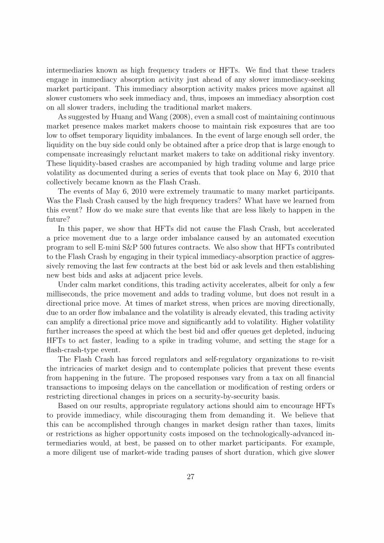
To test whether or not HFTs and Market Makers changed their behavior on the dayof the Flash Crash, we interact dummy variables for the Up phase and the Down phaseof the Flash Crash with the regression coefficients in equation 2. Letting DD

t denote adummy variable for the Down phase (13:32:00 to 13:45:28 CT) and DU

t a dummy variablefor the Up phase (13:45:33 to 14:08:00 CT), the regression specification becomes:

∆yt = α + φ∆yt−1 + δyt−1 + Σ20i=0[βi × pt−i/0.25]

+DDt {αD + φD∆yt−1 + δDyt−1 + Σ20

i=0[βDi × pt−i/0.25]}

+DUt {αU + φU∆yt−1 + δUyt−1 + Σ20

i=0[βUi × pt−i/0.25]}+ εt,

We stack observations from May 3, May 4, May 5, and May 6 (excluding only theobservations after 14:08:00 (CT)). By creating two sets of dummy variables for the downand up periods of the Flash Crash, we test for a change in trading behavior relative tothe rest of the sample period. With this approach, we are able to estimate any changeof behavior by HFTs and Market Makers during the Flash Crash. Results are presentedin the table below.

<Insert Table IV >

For HFTs, during the Down Phase, all coefficients except for one are statisticallyinsignificant. We interpret this as evidence that HFTs did not (either economically orstatistically) significantly change their trading behavior during the Down phase, i.e. thetime when the prices were rapidly falling. We also find that during the Up phase whichcommenced after a 5 second pause in trading, the coefficients for the contemporaneousprice change as well as two seconds prior to it are negative and significant for HFTs.This suggests that during the Up phase, HFTs reduced their inventory 2 seconds prior toand contemporaneously with price increases. In summary, during the critical 36 minutesof the Flash Crash, HFTs are not changing their behavior when prices are falling andseem to be selling as prices are rising relative to the rest of the sample.

In contrast, Market Makers, increase their inventory during several seconds in theDown phase and then reduce their inventory 1 second prior to and contemporaneouslywith price decreases relative to the rest of the sample. Furthermore, Market Makersreduce their inventory between the 10th and the 3rd second in the Up phase and thenturn around and increase their inventory 1 second prior to and contemporaneously withprice increases relative to the rest of the sample. This empirical pattern suggests that

14

Market Makers accumulated inventories on the way down, temporarily got run over mythe fall in prices, then kept buying in the up period. This is consistent with liquidityprovision leading up to and during a market dislocation. However, Market Makers aresimply being overwhelmed by a very large liquidity imbalance that we examine in thenext section.

IV. Absorbing a Large Order Flow Imbalance

There are strong theoretical reasons to believe that a large order flow imbalance cantrigger a market crash even in the absence of any fundamental shock by overwhelmingthe limited risk-bearing capacity of the intermediaries.10 The important aspect of theFlash Crash is how quickly the prices in the E-mini have recovered to the pre-crash levelsas liquidity rushed into the market attracted by lower prices. Which traders suppliedthe liquidity in response to an order flow imbalance merely an hour before the stockmarket closes, when and how did it happen, and why did the trading volume spike up?

To empirically investigate these questions, we divide the 36-minute Flash Crashinto two phases – 13 minutes of rapidly declining prices (from 2:32 p.m. to 2:45 p.m.ET) followed by 23 minutes of rapidly increasing prices (from 2:45 p.m. to 3:08 p.m.ET). Figure 5 plots minute-by-minute net purchases and sales by Fundamental Buyers,Fundamental Sellers, and Opportunistic Traders from the period starting 15 minutesbefore the down phase of the Flash Crash until the end of the up phase.

<Insert Figure 5 >

During the down phase of the Flash Crash, Fundamental Sellers were frequently sell-ing more than 5,000 contracts per minute ($250 million). In the minutes surroundingthe bottom of the Flash Crash, sales by Fundamental Sellers reached 10,000 to 20,000contracts per minute ($500 million to $1 billion). At the same time, purchases by Fun-damental Buyers were significantly smaller than sales by Fundamental Sellers with thebalance being acquired by the Opportunistic Traders. At the beginning of the up phase,Fundamental Sellers continued to sell heavily. Fundamental Buyers absorbed some ofthe selling pressure with remainder going again to Opportunistic Traders. Towards theend of the up phase, Opportunistic Traders both bought and sold in different minutes,on average liquidating some of the purchases they had made earlier.

Table V presents total purchases and sales by the six trader categories during thedown- and up-phases of the Flash Crash on May 6 (panel A) with average quantities forthe three previous days May 3-5 (panel B).

<Insert Table V >

10See, for example, Huang and Wang (2008).

15

During the down phase, Fundamental Sellers made gross sales of 94,101 contracts(net sales of 83,599 contracts), while Fundamental Buyers made gross purchases of 78,359contracts (net purchases of 49,665 contracts). These quantities are 10 to 15 time largerthan the gross sales of 8,428 and gross purchases of 7,958 made by Fundamental Sellersand Fundamental Buyers during the same period of May 3-5. During the down phase,gross purchases and sales by Opportunistic Traders increased from 20,552 and 20,049contracts during May 3-5 to 221,236 and 189,790 contracts on May 6.

During the up phase, Fundamental Sellers made gross sales of 145,396 contracts (netsales of 110,177), while Fundamental Buyers made gross purchases of 165,612 contracts(net purchases of 110,369 contracts). These quantities also exceed the average grosssales of 15,585 contracts and gross purchases of 14,910 contracts by similar multiplesduring the same time interval of May 3-5. During the up phase, gross purchases andsales by Opportunistic Traders increased from 39,535 and 37,317 contracts during May3-5 to 306,326 and 302,417 contracts

As the table shows, the process by which the modern automated market is able toabsorb order flow imbalances of such magnitude is a confluence of different responsesfrom all six groups of traders. Together, these responses resulted in a 14-fold increase intrading volume compared to the size of the 75,000 contract sell program. This massiveincrease in trading volume indicates how automated markets typically digest order flowimbalances. A small order flow imbalance might generate a tiny increase in intermedi-ation trades, perhaps a few trades by a High Frequency trader or a Market Maker. Incontrast, a large buy or sell program generates many intermediation trades leading tosignificant price adjustments and an increase in trading volume many times the size ofthe order that triggered the imbalance. This occurs because different types of tradershave different strategies: some follow trends while others trade on mean reversion; somehold inventory for mere seconds, while others hold it for minutes, hours, or days. As aresult, contracts are passed around from trader to trader before the order flow imbalanceplays itself out and the price adjustment is completed.

During the down phase of the Flash Crash, High Frequency Traders traded faster thanall other traders, and by doing so have amplified downward price momentum as pricesapproached intraday lows. After buying 3,000 contracts in a falling market in the firstten minutes of the Flash Crash, some High Frequency Traders began to aggressively hitthe bids in the limit order book. Especially in the last minute of the down phase, many ofthe contracts sold by High Frequency Traders looking to aggressively reduce inventorieswere executed against other High Frequency Traders, generating a “hot potato” effectand a rapid spike in trading volume. This is consistent with the fact that High FrequencyTraders as a group did not significantly change their total inventory even as the priceswere rapidly falling.

Figure 6 shows the magnitude of the hot potato effect. The figure presents the 5second moving average of the ratio of the absolute value of the net position change ofHigh Frequency Traders to their trading volume.

16

<Insert Figure 6>

We find that compared to the previous three days, HFT “hot potato” trading on May6 was extremely high. The hot potato effect was especially pronounced between 13:45:13and 13:45:27 CT, when prices were plunging with a tremendous velocity. During thistime, the HFTs traded over 27,000 contracts or about 49% of the total trading volume,but their net position changed by a mere 200 contracts.

The downward spiral in prices and the spike in trading volume were interrupted by afive-second trading pause triggered by the “stop-logic” functionality built into the CME’sGlobex trading system.11 A few seconds after the 5-second pause, transaction prices firststabilized and then rebounded rapidly, as Fundamental Buyers and Opportunistic Traderlifted offers. By 2:08 p.m. CT, 36 minutes after the Flash Crash began, prices of E-minifutures had recovered to their pre-Flash-Crash levels.

Note that the process of absorbing large order flow imbalances in automated mar-kets is quite different from that in open outcry markets. In open outcry markets, marketmakers were actively discouraged from trading with each other and a single trader wish-ing to accumulate a large inventory over a short period of time would be directed mymarket surveillance to trade “upstairs” so as not to destabilize the market. In contrast,in automated markets, trading is anonymous and safeguards are designed to police forindividual order imbalances (e.g., price limits and quantity bands for each order), butnot for large order imbalances or market disruptions that might be caused by a tradingprogram consisting of many individual orders that individually satisfy the safeguardsin place (as was the case with the 75,000 trading program). As a result, open outcrymarkets did not need to employ market-wide stop-logic type functionality to detect anddeal with significant order flow imbalances.

This leads us to suggest that automated exchanges should consider including a num-ber of different functionalities to slow down or pause order matching, especially if signif-icant order flow imbalances are detected. These short pauses followed by auction-basedre-opening procedures would, in the spirit of Huang and Wang (2010), force marketparticipants to coordinate their liquidity supply responses in a pre-determined mannerinstead of seeking to execute ahead of others. We believe that more diligent use of trad-ing pauses of short duration and coordinated re-opening protocols can be an effective

11The CME’s Globex stop-logic functionality is an automated pre-trade safeguard procedure designedto prevent the execution of cascading stop orders that would cause “excessive” declines or increases inprices due to lack of sufficient depth in the central limit order book. In the context of this functionality,“excessive” is defined as being outside of a pre-determined ‘no bust’ range. The ‘no bust range’ variesfrom contract to contract; for the E-mini it was set at 6 index points–24 ticks–in either direction for theE-mini. After the stop-logic functionality is triggered, the trading is paused for a certain period of timeas the matching engine goes in what’s called a ‘reserve state’. The length of the trading pause variesbetween 5 and 20 seconds from contract to contract; it was set at 5 seconds for the E-mini. During the‘reserve state’, orders can be submitted, modified or cancelled, but no executions can take place. Thematching engine exits the reserve state by initiating the same auction opening procedure as it does inthe beginning of each trading day. After the starting price is determined by the re-opening auction, thematching engine goes back into the standard continuous matching protocol.

17

pre-trade safeguard in today’s fast automated markets. The five-second trading pausetriggered at the bottom of the Flash Crash followed by a re-opening auction procedureis one example of such a functionality. The five-second trading pause triggered at thebottom of the Flash Crash followed by a re-opening auction procedure is one example ofsuch a functionality. Many more such “forced coordination” measures could be designedand implemented in today’s fast and interlinked markets.

V. What Do High Frequency Traders Do?

So far, we have established that High Frequency Traders did not trigger the Flash Crash,but have exacerbated the price movement and fueled a spike in the total trading volumeduring the time when the E-mini prices were falling rapidly in response to large orderflow imbalance. What kind of trading activity would make the HFTs contribute thisway to a flash-crash-type event?

We believe that in the ordinary course of business, HFTs use their technologicaladvantage to profit from aggressively removing the last few contracts at the best bidand ask levels and then establishing new best bids and asks at adjacent price levelsahead of an immediacy-demanding customer. As an illustration of this “immediacyabsorption” activity, consider the following stylized example, presented in Figure 7 anddescribed below.

<Insert Figure 7>

Suppose that we observe the central limit order book for a stock index futures con-tract. The notional value of one stock index futures contract is $50. The market is veryliquid – on average there are hundreds of resting limit orders to buy or sell multiplecontracts at either the best bid or the best offer. At some point during the day, dueto temporary selling pressure, there is a total of just 100 contracts left at the best bidprice of 1000.00. Recognizing that the queue at the best bid is about to be depleted,HFTs submit executable limit orders to aggressively sell a total of 100 contracts, thuscompletely depleting the queue at the best bid, and very quickly submit sequences ofnew limit orders to buy a total of 100 contracts at the new best bid price of 999.75,as well as to sell 100 contracts at the new best offer of 1000.00. If the selling pressurecontinues, then HFTs are able to buy 100 contracts at 999.75 and make a profit of $1,250dollars among them. If, however, the selling pressure stops and the new best offer priceof 1000.00 attracts buyers, then HFTs would very quickly sell 100 contracts (which areat the very front of the new best offer queue), “scratching” the trade at the same priceas they bought, and getting rid of the risky inventory in a few milliseconds.

This type of trading activity reduces, albeit for only a few milliseconds, the latencyof a price move. Under normal market conditions, this trading activity somewhat accel-erates price changes and adds to the trading volume, but does not result in a significant

18

directional price move. In effect, this activity imparts a small “immediacy absorption”cost on all traders, including the market makers, who are not fast enough to cancel thelast remaining orders before an imminent price move.

This activity, however, makes it both costlier and riskier for the slower market mak-ers to maintain continuous market presence. In response to the additional cost and risk,market makers lower their acceptable inventory bounds to levels that are too small to off-set temporary liquidity imbalances of any significant size. When the diminished liquiditybuffer of the market makers is pierced by a sudden order flow imbalance, they begin todemand a progressively greater compensation for maintaining continuous market pres-ence, and prices start to move directionally. Just as the prices are moving directionallyand volatility is elevated, immediacy absorption activity of HFTs can exacerbate a di-rectional price move and amplify volatility. Higher volatility further increases the speedat which the best bid and offer queues are being depleted, inducing HFT algorithms todemand immediacy even more, fueling a spike in trading volume, and making it morecostly for the market makers to maintain continuous market presence. This forces morerisk averse market makers to withdraw from the market, which results in a full-blownmarket crash.

Empirically, immediacy absorption activity of the HFTs should manifest itself in thedata very differently from the liquidity provision activity of the Market Makers. Toestablish the presence of these differences in the data, we test the following hypotheses:

Hypothesis H1: HFTs are more likely than Market Makers to aggressively executethe last 100 contracts at the best bid or offer before a price move in the direction of thetrade. Market Makers are more likely than HFTs to have the last 100 resting contractsagainst which aggressive orders are executed.

Hypothesis H2: HFTs trade aggressively in the direction of the price move, thenreverse position with passive trade. Market Makers get run over by a price move.

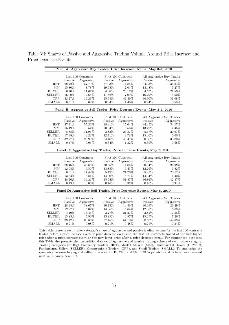
Hypothesis H3: Both HFTs and Market Makers scratch trades, but HFTs scratchmore.

To statistically test our “immediacy absorption” hypotheses against the “liquidityprovision” hypotheses, we divide all of the trades during the 405 minute trading dayinto two subsets: Aggressive Buy trades and Aggressive Sell trades. A specific trade isoften not a standalone event, but a part of a sequence of transactions associated withthe execution of a particular trading strategy. Looking at the sequence of trades ratherthan the individual trades allows us to make inferences about the strategies of traders.

Testing Hypothesis H1. Aggressive removal of the last 100 contracts byHFTs; passive provision of the last 100 resting contracts by the MarketMakers. Using the Aggressive Buy sequences, we label as a “price increase event” alloccurrences of trading sequences in which at least 100 contracts consecutively executedat the same price are followed by some number of contracts at a higher price. Toexamine indications of low latency, we focus on the last 100 contracts traded before theprice increase and the first 100 contracts at the next higher price (or fewer if the price

19

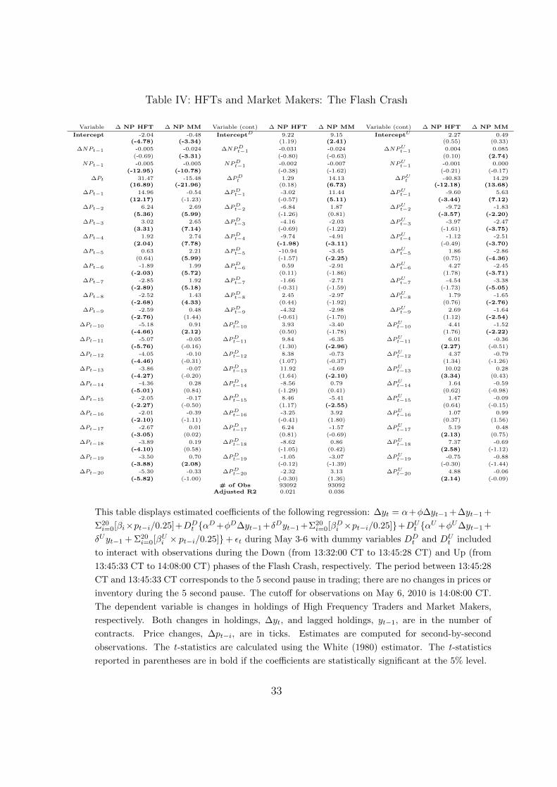
changes again before 100 contracts are executed). Although we do not look directly atthe limit order book data, price increase events are defined to capture occasions wheretraders use executable buy orders to lift the last remaining best offers in the limit orderbook. Using Aggressive sell trades, we define “price decrease events” symmetrically asoccurrences of sequences of trades in which 100 contracts executed at the same price arefollowed by executions at lower prices. These events are intended to capture occasionswhere traders use executable sell orders to hit the last few best bids in the limit orderbook. The results are presented in Table VI.

<Insert Table VI>

Table VI has four panels covering (A) price increase events on May 3-5, (B) pricedecrease events on May 3-5, (C) price increase events on May 6, and (D) price decreaseevents on May 6. In each panel there are six rows of data, one row for each tradercategory. Relative to panels A and C, the rows for Fundamental Buyers (BUYER)and Fundamental Sellers (SELLER) are reversed in panels B and D to emphasize thesymmetry between buying during price increase events and selling during price decreaseevents. The first two columns report the percentage shares of Aggressive and Passivecontract volume for up to the last 100 contracts before the price change; the next twocolumns report the percentage shares of Aggressive and Passive volume for up to thenext 100 contracts after the price change. For comparison, the last two columns reportthe “unconditional” market shares of Aggressive and Passive sides of all Aggressive buyvolume or sell volume. For May 3-5, the data are based on volume pooled across thethree days.

During May 3-5, there were 4100 price increase events and 4062 price decrease events.On May 6 alone, there were 4101 price increase events and 4377 price decrease events.Similarity in the number of price events is consistent with our treating the period ofMay 3-5 as a “single day” when comparing it to May 6.

The percentage share of Aggressive and Passive contract volume for up to the last100 contracts before the price change is calculated as follows: starting at a price changeevent, we count backwards the number of contracts traded at the “old” price precedingthe price event; when we get to 100 contracts and there was not another price event,we stop; if there is another price event fewer than 100 contracts back, we also stop; wethen attribute each contract traded either Aggressively or Passively to one of our sixcategories of traders, add up the contracts for each category, and calculate the percentageshare of Aggressive and Passive contract volume for up to the last 100 contracts tradedat the “old” price before the price change. We then compute averages for each categoryover all price increase and all price decrease events for May 3-5 and May 6, respectively.

Similarly, we calculate the percentage shares of Aggressive and Passive volume forup to the next 100 contracts after the price change by counting forward the numberof contracts traded at the “new” price following the price event. Again, if there no

20

subsequent price event, we stop at 100 contracts; if there is another price event fewerthat 100 contracts forward, we stop at whatever the number contracts (less than 100) wastraded at the “new” price. We then attribute each contract traded either Aggressively orPassively to one of our six categories of traders, add up the contracts for each category,and calculate the percentage share of Aggressive and Passive contract volume for upto the next 100 contracts traded at the “new” price after the price change. We thencompute averages for each category over all price increase and all price decrease eventsfor May 3-5 and May 6, respectively.

For robustness, we conducted the same analysis for 20 and 50 contracts, as well as for10, 25, and 50 transactions (on average there are [4] contracts are traded per transaction)and came up with qualitatively similar results. Furthermore, standard errors associatedwith the averages for “up to the last 100” or “up to the next 100” contracts are alwaysless than 1%. For that reason, we do not report them in the table.

Consider panel A of Table VI, which describes price increase events associated withAggressive buy trades on May 3-5, 2010. High Frequency Traders participated on theAggressive side of 34.04% of all aggressive buy volume. Strongly consistent with ourimmediacy absorption hypothesis, the participation rate rises to 57.70% of the Aggressiveside of trades on the last 100 contracts of Aggressive buy volume before price increaseevents and falls to 14.84% of the Aggressive side of trades on the first 100 contracts ofAggressive buy volume after price increase events.

High Frequency Traders participated on the Passive side of 34.33% of all aggressivebuy volume. Consistent with our hypothesis, the participation rate on the Passive sideof Aggressive buy volume falls to 28.72% of the last 100 contracts before a price increaseevent. It rises to 37.93% of the first 100 contracts after a price increase event.

These results are inconsistent with the notion that High Frequency Traders behavelike textbook market makers, suffering adverse selection losses associated with beingpicked off by informed traders. Instead, when the price is about to move to a new level,HFTs tend to avoid being run over and take the price to the new level with Aggressivetrades of their own.

Market Makers follow a noticeably more passive trading strategy than High Fre-quency Traders. According to panel A or Table VI, Market Makers are 13.48% of thePassive side of all Aggressive trades, but they are only 7.27% of the Aggressive sideof all Aggressive trades. On the last 100 contracts at the old price, Market Makers’share of volume increases only modestly, from 7.27% to 8.78% of trades. Their shareof Passive volume at the old price increases, from 13.48% to 15.80%. These facts areconsistent with the interpretation that Market Makers, unlike High Frequency Traders,do engage in a strategy similar to traditional passive market making, buying at the bidprice, selling at the offer price, and suffering losses when the price moves against them.These facts are also consistent with our hypothesis that High Frequency Traders havelower latency than Market Makers.

Intuition might suggest that Fundamental Buyers would tend to place the Aggressivetrades which move prices up from one tick level to the next. This intuition does not

21

seem to be corroborated by the data. According to panel A of Table VI, FundamentalBuyers are 21.53% of all Aggressive trades but only 11.61% of the last 100 Aggressivecontracts traded at the old price. Instead, Fundamental Buyers increase their share ofAggressive buy volume to 26.17% of the first 100 contracts at the new price.

Taking into account symmetry between buying and selling, panel B of Table VI showsthe results for Aggressive sell trades during May 3-5, 2010, are almost the same as theresults for Aggressive buy trades. High Frequency Traders are 34.17% of all Aggressivesell volume, increase their share to 55.20% of the last 100 Aggressive sell contracts at theold price, and decrease their share to 15.04% of the last 100 Aggressive sell contracts atthe new price. Market Makers are 7.45% of all Aggressive sell contracts, increase theirshare to only 8.57% of the last 100 Aggressive sell trades at the old price, and decreasetheir share to 6.58% of the last 100 Aggressive sell contracts at the new price. Funda-mental Sellers’ shares of Aggressive sell trades behave similarly to Fundamental Buyers’shares of Aggressive Buy trades. Fundamental Sellers are 20.91% of all Aggressive sellcontracts, decrease their share to 11.96% of the last 100 Aggressive sell contracts at theold price, and increase their share to 24.87% of the first 100 Aggressive sell contracts atthe new price.

Panels C and D of Table VI report results for Aggressive Buy trades and AggressiveSell trades for May 6, 2010. Taking into account symmetry between buying and selling,the results for Aggressive buy trades in panel C are very similar to the results forAggressive sell trades in panel D. For example, Aggressive sell trades by FundamentalSellers were 17.55% of Aggressive sell volume on May 6, while Aggressive buy trades byFundamental Buyers were 20.12% of Aggressive buy volume on May 6. In comparisonwith the share of Fundamental Buyers and in comparison with May 3-5, the Flash Crashof May 6 is associated with a slightly lower—not higher—share of Aggressive sell tradesby Fundamental Sellers.

A comparison of May 6 with May 3-5 reveals that the share of Aggressive trades byHigh Frequency Traders drops from 34.04% of Aggressive buys and 34.17% of Aggressivesells on May 3-5 to 26.98% of Aggressive buy trades and 26.29% of Aggressive sell tradeson May 6. The share of Aggressive trades for the last 100 contracts at the old pricedeclines by even more. High Frequency Traders’ participation rate on the Aggressiveside of Aggressive buy trades drops from 57.70% on May 3-5 to only 38.86% on May6. Similarly, the participation rate on the Aggressive side of Aggressive sell tradesdrops from and 55.20% to 38.67%. These declines are largely mimicked by increases inthe participation rate by Opportunistic Traders on the Aggressive side of trades. Forexample, Opportunistic Traders’ share of the Aggressive side of the last 100 contractstraded at the old price rises from 19.21% to 34.26% for Aggressive buys and from 20.99%to 33.86% for Aggressive sells. These results likely come about because OpportunisticTraders engaged in cross-market arbitrage strategies (e.g., trading the E-mini againstthe SPY - S&P 500 ETF) were extremely active during the Flash Crash as evidencedby the propagation of the shock from the E-mini to the SPY (which is what made theFlash Crash a systemic event).

22

Testing Hypothesis H2. HFTs trade aggressively in the direction of theprice move, then reverse position with a passive trade; Market Makers getrun over by a price move. To examine this hypothesis, we analyze whether HighFrequency Traders use Aggressive trades to trade in the direction of contemporaneousprice changes, while Market Makers use Passive trades to trade in the opposite directionfrom price changes. To this end, we estimate the regression Equation 1 for Passive andAggressive inventory changes separately.

<Insert Table VII >

Table VII presents the regression results of the two components of change in hold-ings on lagged inventory, lagged change in holdings and lagged price changes over onesecond intervals. Panel A and Panel B report the results for May 3-5 and May 6,respectively. Each panel has four columns, reporting estimated coefficients where thedependent variables are net Aggressive volume (Aggressive buys minus Aggressive sells)by High Frequency Traders (∆AHFT ), net Passive volume by High Frequency Traders(∆P HFT ), net Aggressive volume by Market Makers (∆AMM), and net Passive vol-ume by Market Makers (∆P MM).

We observe that for lagged inventories (NPHFTt−1), the estimated coefficients forAggressive and Passive trades by High Frequency Traders are δAHFT = −0.005 (t =−9.55) and δP HFT = −0.001 (t = −3.13), respectively. These coefficient estimateshave the interpretation that High Frequency Traders use Aggressive trades to liquidateinventories more intensively than passive trades. In contrast, the results for MarketMakers are very different. For lagged inventories (NPMMt−1), the estimated coefficientsfor Aggressive and Passive volume by Market Makers are δAMM = −0.002 (t = −6.73)and δP MM = −0.002 (t = −5.26), respectively. The similarity of these coefficientsestimates has the interpretation that Market Makers favor neither Aggressive trades norPassive trades when liquidating inventories.

For contemporaneous price changes (in the current second) (∆Pt−1), the estimatedcoefficient Aggressive and Passive volume by High Frequency Traders are β0 = 57.78(t = 31.94) and β0 = −25.69 (t = −28.61), respectively. For Market Makers, theestimated coefficients for Aggressive and Passive trades are β0 = 6.38 (t = 18.51) andβ0 = −19.92 (t = −37.68). These estimated coefficients have the interpretation thatin seconds in which prices move up one tick, High Frequency Traders are net buyersof about 58 contracts with Aggressive trades and net sellers of about 26 contracts withPassive trades in that same second, while Market Makers are net buyers of about 6contracts with Aggressive trades and net sellers of about 20 contracts with Passivetrades. High Frequency Traders and Market Makers are similar in that they both useAggressive trades to trade in the direction of price changes, and both use Passive tradesto trade against the direction of price changes. High Frequency Traders and MarketMakers are different in that Aggressive net purchases by High Frequency Traders are

23

greater in magnitude than the Passive net purchases, while the reverse is true for MarketMakers.

For lagged price changes, coefficient estimates for Aggressive trades by High Fre-quency Traders and Market Makers are positive and statistically significant at lags 1-4and lags 1-10, respectively. These results have the interpretation that both High Fre-quency Traders’ and Market Makers’ trade on recent price momentum, but the tradingis compressed into a shorter time frame for High Frequency Traders than for MarketMakers.

For lagged price changes, coefficient estimates for Passive volume by High FrequencyTraders and Market Makers are negative and statistically significant at lags 1 and lags1-3, respectively.12

Panel B of Table VII presents results for May 6. Similar to May 3-5, High FrequencyTraders tend to use Aggressive trades more actively than Passive trades to liquidateinventories, while Market Makers do not show this pattern. Also similar to May 3-5,High Frequency Trades and Market Makers use Aggressive trades to trade in the con-temporaneous direction of price changes and use Passive trades to trade in the directionopposite price changes, with Aggressive trading greater than Passive trading for HighFrequency Traders and the reverse for Market Makers. In comparison with May 3-5, thecoefficients are smaller in magnitude on May 6, indicating reduced liquidity at each tick.For lagged price changes, the coefficients associated with Aggressive trading by HighFrequency Traders change from positive to negative at lags 1-4, and the positive coeffi-cients associated with Aggressive trading by Market Makers change from being positiveand statistically significant at lags 1-10 to being positive and statistically significant onlyat lags 1-3. These results illustrate accelerated trading velocity in the volatile marketconditions of May 6.

We further examine how high frequency trading activity is related to market prices.Figure 8 illustrates how prices change after HFT trading activity in a given second.The upper-left panel presents results for buy trades for May 3-5, the upper right panelpresents results for buy trades on May 6, and the lower-left and lower-right presentcorresponding results for sell trades. For an “event” second in which High FrequencyTraders are net buyers, net Aggressive Buyers, and net Passive Buyers, value-weightedaverage prices paid by the High Frequency Traders in that second are subtracted fromthe value-weighted average prices for all trades in the same second and each of thefollowing 20 seconds. The results are averaged across event seconds, weighted by themagnitude of High Frequency Traders’ net position change in the event second. Pricedifferences on the vertical axis are scaled so that one unit equals one tick ($12.50 perone E-mini contract).

12We also introduce lead price changes up to 10 seconds into this regression framework. Price changecoefficients are positive and significant for the net aggressive volume of High Frequency Traders beforeMay 6. Coefficients are very similar when we include longer lags of prices and holdings changes. Newey-West standard errors are very close to White standard errors. Results are available upon request.

24

<Insert Figure 8>

When High Frequency Traders are net buyers during May 3-5, prices rise by 17% of atick in the next second, then begin to gradually fall; 20 seconds after a net buy by HFTs,process remain 15 % of a tick higher. The total effect of net buy HFT trades can beseparated into net aggressive and net passive buy trades. When HFTs buy aggressively,prices rise by 20% of a tick in the next second, continue rising into the next second,stabilize at about 23

On May 6, the effects of an aggressive HFT buy trade and a passive HFT sell tradeare qualitatively the same as during May 3-5. However, the permanent price effects ofHFT trading on that day are much more pronounced for an aggressive HFT sell or apassive HFT buy. Following an aggressive HFT sell, prices continue to drift down forthe next 20 seconds (when they reach over half a tick); similarly, prices continue to driftupward after a passive HFT buy until they stabilize at stay at about half a tick 20seconds later.

These charts illustrate how profitable the “immediacy removal” trading strategy isfor HFTs. During May 3-5, HFTs make about a quarter of a tick per contract withinseconds by either aggressively selling and then passively buying (before a price move) orby aggressively buying and then passively selling (when the price comes to their restingorders). During the times of fast changing prices and very high volatility, HFTs make afull tick per contract in a matter of seconds.

Testing Hypothesis H3. Both HFTs and Market Makers scratch trades;HFTs scratch more. A textbook market maker will try to buy at the bid price, sellat the offer price, and capture the bid-ask spread as a profit. Sometimes, after buyingat the bid price, market prices begin to fall before the market maker can make a onetick profit by selling his inventory at the best offer price. To avoid taking losses in thissituation, one component of a traditional market making strategy is to “scratch trades inthe presence of changing market conditions by quickly liquidating a position at the sameprice at which it was acquired. These scratched trades represent inventory managementtrades designed to lower the cost of adverse selection. Since many competing marketmakers may try to scratch trades at the same time, traders with the lowest latency willtend to be more successful in their attempts to scratch trades and thus more successfulin their ability to avoid losses when market conditions change.

To examine whether and to what extent traders engage in trade scratching, we se-quence each trader’s trades for the day using audit trail sequence numbers which notonly sort trades by second but also sort trades chronologically within each second. Wedefine an “immediately scratched trade” as a trade with the properties that the nexttrade in the sorted sequence (1) occurred in the same second, (2) was executed at thesame price, (3) was in the opposite direction, i.e., buy followed by sell or sell followedby buy. For each of the trading accounts in our sample, we calculate the number of

25

immediately scratched trades, then compare the number of scratched trades across thesix trader categories.

The results of this analysis are presented in the table below. Panel A provides resultsfor May 3-5 and panel B for May 6. In each panel, there are five rows of data, one foreach trader category. The first three columns report the total number of trades, thetotal number of immediately scratched trades, and the percentage of trades that areimmediately scratched by traders in five categories. Small trader category results arenot reported for confidentiality reasons. For May 3-6, the reported numbers are fromthe pooled data.

<Insert Table VIII>

This table shows that High Frequency Traders scratched 2.84 % of trades on May 3-5 and 4.26 % on May 6; Market Makers scratched 2.49 % of trades on May 3-5 and5.53 % of trades on May 6. While the percentages of immediately scratched trades byMarket Makers is slightly higher than that for High Frequency Traders on May 6, thepercentages for both groups are very similar.

The fourth, fifth, and sixth columns of Table VIII report the mean, standard devia-tion, and median of the number of scratched trades for the traders in each category.

Although the percentages of scratched trades are similar, the mean number of im-mediately scratched trades by High Frequency Traders is much greater than for MarketMakers: 540.56 per day on May 3-5 and 1610.75 on May 6 for High Frequency Tradersversus 13.35 and 72.92 for Market Makers. The differences between High FrequencyTraders and Market Makers reflect differences in volume traded. Table VIII shows thatHigh Frequency Traders and Market Makers scratch a significantly larger percentage oftheir trades than other trader categories.

VI. Concluding Remarks

More than 40 years ago, stock exchanges began to think about switching from face-to-face human trading to fully automated trading platforms. Fischer Black (1971) surmisedthat, regardless of whether markets were human or automated, liquid markets wouldexhibit price continuity only if trading is characterized by a large volume of small in-dividual trades. As electronic central limit order books have replaced human trading,Black’s insights have proven to be correct. Black (1995) also predicted that, to reduceimpact costs, electronic markets would induce institutions to shift from executing largetrades as blocks with “upstairs” human dealers to using “order shredding” strategies inwhich computer algorithms submit many small trades over time into electronic tradingplatforms. This insight has also proven to be correct.

Black did not foresee, however, how dramatically advances in the computing andtelecommunication technology would favor the most technologically-advanced financial

26

intermediaries known as high frequency traders or HFTs. We find that these tradersengage in immediacy absorption activity just ahead of any slower immediacy-seekingmarket participant. This immediacy absorption activity makes prices move against allslower customers who seek immediacy and, thus, imposes an immediacy absorption coston all slower traders, including the traditional market makers.

As suggested by Huang and Wang (2008), even a small cost of maintaining continuousmarket presence makes market makers choose to maintain risk exposures that are toolow to offset temporary liquidity imbalances. In the event of large enough sell order, theliquidity on the buy side could only be obtained after a price drop that is large enough tocompensate increasingly reluctant market makers to take on additional risky inventory.These liquidity-based crashes are accompanied by high trading volume and large pricevolatility as documented during a series of events that took place on May 6, 2010 thatcollectively became known as the Flash Crash.

The events of May 6, 2010 were extremely traumatic to many market participants.Was the Flash Crash caused by the high frequency traders? What have we learned fromthis event? How do we make sure that events like that are less likely to happen in thefuture?

In this paper, we show that HFTs did not cause the Flash Crash, but accelerateda price movement due to a large order imbalance caused by an automated executionprogram to sell E-mini S&P 500 futures contracts. We also show that HFTs contributedto the Flash Crash by engaging in their typical immediacy-absorption practice of aggres-sively removing the last few contracts at the best bid or ask levels and then establishingnew best bids and asks at adjacent price levels.

Under calm market conditions, this trading activity accelerates, albeit for only a fewmilliseconds, the price movement and adds to trading volume, but does not result in adirectional price move. At times of market stress, when prices are moving directionally,due to an order flow imbalance and the volatility is already elevated, this trading activitycan amplify a directional price move and significantly add to volatility. Higher volatilityfurther increases the speed at which the best bid and offer queues get depleted, inducingHFTs to act faster, leading to a spike in trading volume, and setting the stage for aflash-crash-type event.

The Flash Crash has forced regulators and self-regulatory organizations to re-visitthe intricacies of market design and to contemplate policies that prevent these eventsfrom happening in the future. The proposed responses vary from a tax on all financialtransactions to imposing delays on the cancellation or modification of resting orders orrestricting directional changes in prices on a security-by-security basis.

Based on our results, appropriate regulatory actions should aim to encourage HFTsto provide immediacy, while discouraging them from demanding it. We believe thatthis can be accomplished through changes in market design rather than taxes, limitsor restrictions as higher opportunity costs imposed on the technologically-advanced in-termediaries would, at best, be passed on to other market participants. For example,a more diligent use of market-wide trading pauses of short duration, which give slower

27

algorithms a few much needed seconds to decide on what terms they are willing toreplenish liquidity in the central limit order book, can be a highly effective pre-tradesafeguard in today’s fast and interlinked markets.

We acknowledge that in markets for individual securities, fragmentation of order flowacross competing trading venues makes the coordination of brief trading pauses difficult.We also acknowledge that the task of coordinating responses across competing marketsoverseen by different regulators with contradictory objectives is even more difficult. Thispaper is our call to rise to these challenges.

28

References

Black, Fischer, 1971, Towards a Fully Automated Exchange, Part I, Financial AnalystsJournal 27, 29-34.

Black, Fischer, 1995, Equilibrium Exchanges, Financial Analysts Journal 51, 23-29.

CFTC-SEC Staff Report, Preliminary Findings Regarding the Market Events of May 6,2010.

CFTC-SEC Staff Report, Findings Regarding the Market Events of May 6, 2010.

Grossman, Sanford J., and Miller, Merton H., 1988, Liquidity and Market Structure,Journal of Finance 43,3,617–633.

Hasbrouck, Joel, 2003, Intraday Price Formation in U.S. Equity Index Markets, Journalof Finance 58, 2375–2400.

Huang, Jennifer. and Jiang Wang, 2008, Liquidity and market crashes, Review ofFinancial Studies, 2607-2643.

Huang, Jennifer and Jiang Wang, 2010, Market Liquidity, Asset Prices, and Welfare,Journal of Financial Economics, 95, 107-127.

White, Halbert, 1980, A Heteroskedasticity-Consistent Covariance Matrix Estimatorand a Direct Test for Heteroskedasticity, Econometrica 48, 817–838.

29

Table I: Market Descriptive Statistics

May 3-5 May 6thDaily Trading Volume 2,397,639 5,094,703

# of Trades 446,340 1,030,204# of Traders 11,875 15,422

Trade Size 5.41 4.99Order Size 10.83 9.76

Limit Orders % Volume 95.45% 92.44%Limit Orders % Trades 94.36% 91.75%

Log High-Low Range 1.54% 9.82%Return -0.02% -3.05%

This table presents summary statistics for the June 2010 E-Mini S&P 500 futures con-

tract. The first column presents averages calculated for May 3-5, 2010 between 8:30 and

15:15 CT. The second column presents statistics for May 6, 2010 between 8:30 to 15:15 CT.

Volume is the number of contracts traded. The number of traders is the number of trading

accounts that traded at least once during a trading day. Order size and trade sizes are

measured in the number of contracts. The use of limit orders is presented both in percent

of the number of transactions and trading volume. Volatility is calculated as range, the

natural logarithm of maximum price over minimum price within a trading day.

30

Tab

leII

:Sum

mar

ySta

tist

ics

ofT

rader

Cat

egor

ies

PanelA:M

ay

3-5

3Day

Average

Tra

der

Typ

e%

Volu

me

%of

Tra

des

#T

rad

ers

Tra

de

Siz

eO

rder

Siz

eL

imit

Ord

ers

Lim

itO

rder

sA

gg

Rati

oA

gg

Rati

o(A

vg.)

(Avg.)

%V

olu

me

%T

rad

esT

rad

e-W

eighte

dV

ol-

Wei

ghte

dH

igh

Fre

qu

ency

Tra

der

s34.2

2%

32.5

6%

15

5.6

914.7

5100.0

00%

100.0

00%

49.9

1%

45.6

8%

Mark

etM

aker

s10.4

9%

11.6

3%

189

4.8

87.9

299.6

14%

98.9

39%

43.1

0%

41.6

2%

Fu

nd

am

enta

lB

uyer

s11.8

9%

10.1

5%

1,0

13

6.3

414.0

991.2

58%

91.2

73%

66.0

4%

64.0

9%

Fu

nd

am

enta

lS

elle

rs12.1

1%

10.1

0%

1,0

88

6.5

014.2

092.1

76%

91.3

60%

62.8

7%

61.1

3%

Op

port

un

isti

cT

rad

ers

30.7

9%

33.3

4%

3,5

04

4.9

88.8

092.1

37%

90.5

49%

55.9

8%

54.7

1%

Sm

all

Tra

der

s0.5

0%

2.2

2%

6,0

65

1.2

21.2

570.0

92%

71.2

05%

59.0

4%

59.0

6%

Volu

me

#of

Tra

des

#T

rad

ers

Tra

de

Siz

eO

rder

Siz

eL

imit

Ord

ers

Lim

itO

rder

sV

ola

tility

Ret

urn

(Avg.)

(Avg.)

%V

olu

me

%T

rad

esA

ll2,3

97,6

39

446,3

40

11,8

75

5.4

110.8

395.4

5%

94.3

6%

1.5

4%

-0.0

2%

PanelB:M

ay

6th

Tra

der

Typ

e%

Volu

me

%of

Tra

des

#T

rad

ers

Tra

de

Siz

eO

rder

Siz

eL

imit

Ord

ers

Lim

itO

rder

sA

gg

Rati

oA

gg

Rati

o(A

vg.)

(Avg.)

%V

olu

me

%T

rad

esT

rad

e-W

eighte

dV

ol-

Wei

ghte

dH

igh

Fre

qu

ency

Tra

der

s28.5

7%

29.3

5%

16

4.8

59.8

699.9

97%

99.9

97%

50.3

8%

45.5

3%

Mark

etM

aker

s9.0

0%

11.4

8%

179

3.8

95.8

899.6

39%

99.2

37%

45.1

8%

43.5

5%

Fu

nd

am

enta

lB

uyer

s12.0

1%

11.5

4%

1,2

63

5.1

510.4

388.8

41%

89.5

89%

64.3

9%

61.0

8%

Fu

nd

am

enta

lS

elle

rs10.0

4%

6.9

5%

1,2

76

7.1

921.2

989.9

85%

88.9

66%

68.4

2%

65.6

8%

Op

port

un

isti

cT

rad

ers

40.1

3%

39.6

4%

5,8

08

5.0

510.0

687.3

85%

85.3

52%

61.9

2%

60.2

8%

Sm

all

Tra

der

s0.2

5%

1.0

4%

6,8

80

1.2

01.2

463.6

09%

64.8

79%

63.4

9%

63.5

3%

Volu

me

#of

Tra

des

#T

rad

ers

Tra

de

Siz

eO

rder

Siz

eL

imit

Ord

ers

Lim

itO

rder

sV

ola

tility

Ret

urn

(Avg.)

(Avg.)

%V

olu

me

%T

rad

esA

ll5,0

94,7

03

1,0

30,2

04

15,4

22

4.9

99.7

692.4

43%

91.7

50%

9.8

2%

-3.0

5%

Th

ista

ble

pre

sents

sum

mar

yst

atis

tics

for

trad

erca

tego

ries

and

the

over

all

mark

et.

Th

efi

rst

colu

mn

pre

sents

stat

isti

csp

rior

toM

ay6

asth

eav

erag

eov

erth

ree

trad

ing

day

s,M

ay3-

5,201

0fr

om8:3

0to

15:

15

CT

.T

he

seco

nd

colu

mn

pre

sents

stati

stic

sfo

rM

ay6

from

8:30

to15

:15

CT

.

31

Table III: HFTs and Market Makers: Net Holdings and Prices

Panel A: May 3-5 Panel B: May 6

∆ NP HFT ∆ NP MM ∆ NP HFT ∆ NP MMIntercept -1.64 -0.53 Intercept -3.22 0.04

(-3.54) (-3.33) (-3.38) (0.13)∆NPHFTt−1 -0.006 ∆NPHFTt−1 0.011

(-0.69) (1.19)NPHFTt−1 -0.005 NPHFTt−1 -0.005

(-11.77) (-6.76)∆NPMMt−1 -0.006 ∆NPMMt−1 -0.035

(-0.79) (-2.69)NPMMt−1 -0.004 NPMMt−1 -0.008

(-8.93) (-7.79)∆Pt 32.09 -13.54 ∆Pt 10.81 -8.16

(18.44) (-23.83) (6.05) (-12.09)∆Pt−1 17.18 -1.22 ∆Pt−1 4.63 6.64

(12.58) (-2.71) (3.39) (13.88)∆Pt−2 8.36 2.16 ∆Pt−2 -1.52 2.73

(7.15) (4.99) (-1.25) (4.44)∆Pt−3 5.09 2.53 ∆Pt−3 -1.36 1.14

(4.93) (5.97) (-1.06) (2.84)∆Pt−4 3.91 2.65 ∆Pt−4 -1.82 0.49

(3.62) (6.54) (-1.48) (1.11)∆Pt−5 1.81 2.50 ∆Pt−5 -0.23 -0.77

(1.56) (5.91) (-1.17) (-1.68)∆Pt−6 -0.08 2.16 ∆Pt−6 -0.31 -0.31

(-0.07) (5.42) (-0.23) (-0.78)∆Pt−7 -1.00 1.84 ∆Pt−7 -5.04 -0.62

(-0.97) (4.96) (-3.62) (-1.33)∆Pt−8 -1.76 1.47 ∆Pt−8 -1.78 -0.36

(-1.56) (3.83) (-1.41) (-0.93)∆Pt−9 -1.81 0.45 ∆Pt−9 -1.68 -1.11

(-1.70) (1.19) (-1.35) (-2.45)∆Pt−10 -3.90 0.52 ∆Pt−10 -1.65 -0.39

(-3.78) (1.37) (-1.13) (-0.84)∆Pt−11 -4.73 -0.03 ∆Pt−11 -1.08 -0.63

(-4.70) (-0.07) (-0.74) (-1.28)∆Pt−12 -3.46 0.15 ∆Pt−12 0.71 -1.17

(-3.33) (0.41) (0.43) (-2.58)∆Pt−13 -3.80 0.27 ∆Pt−13 2.26 -0.62

(-3.74) (0.72) (1.43) (-1.49)∆Pt−14 -4.77 0.32 ∆Pt−14 -2.66 -0.27

(-4.70) (0.86) (-1.85) (-0.71)∆Pt−15 -2.74 -0.19 ∆Pt−15 0.43 -0.83

(-2.63) (-0.53) (0.34) (-2.19)∆Pt−16 -2.21 -0.64 ∆Pt−16 -0.68 0.23

(-2.09) (-1.72) (-0.41) (0.61)∆Pt−17 -2.52 -0.10 ∆Pt−17 -0.66 0.29

(-2.45) (-0.26) (-0.45) (0.73)∆Pt−18 -4.36 0.04 ∆Pt−18 0.45 -0.77

(-3.96 (0.12) (0.29) (-2.04)∆Pt−19 -4.21 0.57 ∆Pt−19 -2.63 -0.30

(-4.16) (1.51) (-1.87) (-0.76)∆Pt−20 -5.86 -0.12 ∆Pt−20 -1.07 -0.71

(-5.86) (-0.33) (-0.79) (-1.65)#obs 72837 72837 #obs 24275 24275

Adj − R2 0.019 0.026 Adj − R2 0.010 0.039

This table displays estimated coefficients of the following regression: ∆yt = α+φ∆yt−1 + δyt−1 +∑20i=0[βi × ∆pt−i/0.25] + εt. The dependent variable is changes in holdings of High Frequency

Traders and Market Makers, respectively. Both changes in holdings, ∆yt, and lagged holdings,

yt−1, are in the number of contracts. Price changes, ∆pt−i, are in ticks. Estimates are computed for

second-by-second observations. The t-statistics are calculated using the White (1980) estimator.

t values reported in parentheses are in bold if the coefficients are statistically significant at the 5%

level. Observations are stacked for May 3-5.

32

Table IV: HFTs and Market Makers: The Flash Crash

Variable ∆ NP HFT ∆ NP MM Variable (cont) ∆ NP HFT ∆ NP MM Variable (cont) ∆ NP HFT ∆ NP MM

Intercept -2.04 -0.48 InterceptD 9.22 9.15 InterceptU 2.27 0.49(-4.78) (-3.34) (1.19) (2.41) (0.55) (0.33)

∆NPt−1 -0.005 -0.024 ∆NPDt−1 -0.031 -0.024 ∆NPU

t−1 0.004 0.085

(-0.69) (-3.31) (-0.80) (-0.63) (0.10) (2.74)

NPt−1 -0.005 -0.005 NPDt−1 -0.002 -0.007 NPU

t−1 -0.001 0.000

(-12.95) (-10.78) (-0.38) (-1.62) (-0.21) (-0.17)

∆Pt 31.47 -15.48 ∆PDt 1.29 14.13 ∆PU

t -40.83 14.29(16.89) (-21.96) (0.18) (6.73) (-12.18) (13.68)

∆Pt−1 14.96 -0.54 ∆PDt−1 -3.02 11.44 ∆PU

t−1 -9.60 5.63

(12.17) (-1.23) (-0.57) (5.11) (-3.44) (7.12)

∆Pt−2 6.24 2.69 ∆PDt−2 -6.84 1.87 ∆PU

t−2 -9.72 -1.83

(5.36) (5.99) (-1.26) (0.81) (-3.57) (-2.20)

∆Pt−3 3.02 2.65 ∆PDt−3 -4.16 -2.03 ∆PU

t−3 -3.97 -2.47

(3.31) (7.14) (-0.69) (-1.22) (-1.61) (-3.75)

∆Pt−4 1.92 2.74 ∆PDt−4 -9.74 -4.91 ∆PU

t−4 -1.12 -2.51

(2.04) (7.78) (-1.98) (-3.11) (-0.49) (-3.70)

∆Pt−5 0.63 2.21 ∆PDt−5 -10.94 -3.45 ∆PU

t−5 1.86 -2.86

(0.64) (5.99) (-1.57) (-2.25) (0.75) (-4.36)

∆Pt−6 -1.89 1.99 ∆PDt−6 0.59 -2.91 ∆PU

t−6 4.27 -2.45

(-2.03) (5.72) (0.11) (-1.86) (1.78) (-3.71)

∆Pt−7 -2.85 1.92 ∆PDt−7 -1.66 -2.71 ∆PU

t−7 -4.54 -3.38

(-2.89) (5.18) (-0.31) (-1.59) (-1.73) (-5.05)

∆Pt−8 -2.52 1.43 ∆PDt−8 2.45 -2.97 ∆PU

t−8 1.79 -1.65

(-2.68) (4.33) (0.44) (-1.92) (0.76) (-2.76)

∆Pt−9 -2.59 0.48 ∆PDt−9 -4.32 -2.98 ∆PU

t−9 2.69 -1.64

(-2.76) (1.44) (-0.61) (-1.70) (1.12) (-2.54)

∆Pt−10 -5.18 0.91 ∆PDt−10 3.93 -3.40 ∆PU

t−10 4.41 -1.52

(-4.66) (2.12) (0.50) (-1.78) (1.76) (-2.22)

∆Pt−11 -5.07 -0.05 ∆PDt−11 9.84 -6.35 ∆PU

t−11 6.01 -0.36

(-5.76) (-0.16) (1.30) (-2.96) (2.27) (-0.51)

∆Pt−12 -4.05 -0.10 ∆PDt−12 8.38 -0.73 ∆PU

t−12 4.37 -0.79

(-4.46) (-0.31) (1.07) (-0.37) (1.34) (-1.26)

∆Pt−13 -3.86 -0.07 ∆PDt−13 11.92 -4.69 ∆PU

t−13 10.02 0.28

(-4.27) (-0.20) (1.64) (-2.10) (3.34) (0.43)

∆Pt−14 -4.36 0.28 ∆PDt−14 -8.56 0.79 ∆PU

t−14 1.64 -0.59

(-5.01) (0.84) (-1.29) (0.41) (0.62) (-0.98)

∆Pt−15 -2.05 -0.17 ∆PDt−15 8.46 -5.41 ∆PU

t−15 1.47 -0.09

(-2.27) (-0.50) (1.17) (-2.55) (0.64) (-0.15)

∆Pt−16 -2.01 -0.39 ∆PDt−16 -3.25 3.92 ∆PU

t−16 1.07 0.99

(-2.10) (-1.11) (-0.41) (1.80) (0.37) (1.56)

∆Pt−17 -2.67 0.01 ∆PDt−17 6.24 -1.57 ∆PU

t−17 5.19 0.48

(-3.05) (0.02) (0.81) (-0.69) (2.13) (0.75)

∆Pt−18 -3.89 0.19 ∆PDt−18 -8.62 0.86 ∆PU

t−18 7.37 -0.69

(-4.10) (0.58) (-1.05) (0.42) (2.58) (-1.12)

∆Pt−19 -3.50 0.70 ∆PDt−19 -1.05 -3.07 ∆PU

t−19 -0.75 -0.88

(-3.88) (2.08) (-0.12) (-1.39) (-0.30) (-1.44)

∆Pt−20 -5.30 -0.33 ∆PDt−20 -2.32 3.13 ∆PU

t−20 4.88 -0.06

(-5.82) (-1.00) (-0.30) (1.36) (2.14) (-0.09)# of Obs 93092 93092

Adjusted R2 0.021 0.036

This table displays estimated coefficients of the following regression: ∆yt = α+φ∆yt−1 +∆yt−1 +

Σ20i=0[βi×pt−i/0.25]+DD

t {αD +φD∆yt−1+δDyt−1+Σ20i=0[βD

i ×pt−i/0.25]}+DUt {αU +φU∆yt−1+

δUyt−1 + Σ20i=0[βU

i × pt−i/0.25]}+ εt during May 3-6 with dummy variables DDt and DU

t included

to interact with observations during the Down (from 13:32:00 CT to 13:45:28 CT) and Up (from

13:45:33 CT to 14:08:00 CT) phases of the Flash Crash, respectively. The period between 13:45:28

CT and 13:45:33 CT corresponds to the 5 second pause in trading; there are no changes in prices or

inventory during the 5 second pause. The cutoff for observations on May 6, 2010 is 14:08:00 CT.

The dependent variable is changes in holdings of High Frequency Traders and Market Makers,

respectively. Both changes in holdings, ∆yt, and lagged holdings, yt−1, are in the number of

contracts. Price changes, ∆pt−i, are in ticks. Estimates are computed for second-by-second

observations. The t-statistics are calculated using the White (1980) estimator. The t-statistics

reported in parentheses are in bold if the coefficients are statistically significant at the 5% level.

33

Table V: Trading Volume During the Flash Crash

Panel A: May 3-5DOWN UP

Sell Buy Net Sell Buy Net

High Frequency Traders 23,746 23,791 45 40,524 40,021 -503Market Makers 6,484 6,328 -156 11,469 11,468 -1Fundamental Buyers 3,064 7,958 4,894 6,127 14,910 8,783Fundamental Sellers 8,428 3,118 -5,310 15,855 5,282 -10,573Opportunistic Traders 20,049 20,552 503 37,317 39,535 2,218Small Traders 232 256 24 428 504 76

Total 62,003 62,003 0 111,720 111,720 0

Panel B: May 6thDOWN UP

Sell Buy Net Sell Buy Net

High Frequency Traders 152,436 153,804 1,368 191,490 189,013 -2,477Market Makers 32,489 33,694 1,205 47,348 45,782 -1,566Fundamental Buyers 28,694 78,359 49,665 55,243 165,612 110,369Fundamental Sellers 94,101 10,502 -83,599 145,396 35,219 -110,177Opportunistic Traders 189,790 221,236 31,446 302,417 306,326 3,909Small Traders 1,032 947 -85 1,531 1,473 -58

Total 498,542 498,542 0 743,425 743,425 0

This table presents the number of contracts sold and bought by trader categories during

DOWN and UP periods. DOWN period is defined as the interval between 13:32:00 and

13:45:28 CT. UP period is defined as the interval between 13:45:33 and 14:08:00 CT.

Panel A reports the average number of contracts bought and sold between May 3 and

May 5, 2010 during the DOWN and UP periods in the day. Panel B reports the number

of contracts bought and sold on May 6, 2010 during the DOWN and UP periods.

34

Table VI: Shares of Passive and Aggressive Trading Volume Around Price Increase andPrice Decrease Events

Panel A: Aggressive Buy Trades, Price Increase Events, May 3-5, 2010

Last 100 Contracts First 100 Contracts All Aggressive Buy TradesPassive Aggressive Passive Aggressive Passive Aggressive

HFT 28.72% 57.70% 37.93% 14.84% 34.33% 34.04%MM 15.80% 8.78% 19.58% 7.04% 13.48% 7.27%

BUYER 6.70% 11.61% 4.38% 26.17% 4.57% 21.53%SELLER 16.00% 2.65% 11.82% 7.09% 16.29% 5.50%

OPP 32.27% 19.21% 25.95% 43.39% 30.90% 31.08%SMALL 0.51% 0.04% 0.34% 1.46% 0.44% 0.58%

Panel B: Aggressive Sell Trades, Price Decrease Events, May 3-5, 2010

Last 100 Contracts First 100 Contracts All Aggressive Sell TradesPassive Aggressive Passive Aggressive Passive Aggressive

HFT 27.41% 55.20% 38.31% 15.04% 34.45% 34.17%MM 15.49% 8.57% 20.64% 6.58% 13.79% 7.45%

SELLER 5.88% 11.96% 3.83% 24.87% 5.67% 20.91%BUYER 17.98% 3.22% 12.71% 8.78% 15.40% 6.00%

OPP 32.77% 20.99% 24.18% 43.41% 30.30% 30.89%SMALL 0.47% 0.06% 0.34% 1.32% 0.39% 0.58%

Panel C: Aggressive Buy Trades, Price Increase Events, May 6, 2010

Last 100 Contracts First 100 Contracts All Aggressive Buy TradesPassive Aggressive Passive Aggressive Passive Aggressive

HFT 28.46% 38.86% 30.55% 14.84% 30.94% 26.98%MM 12.95% 5.50% 13.88% 5.45% 12.26% 5.82%

BUYER 6.31% 17.49% 5.19% 21.76% 5.45% 20.12%SELLER 13.84% 3.84% 14.30% 5.71% 14.34% 4.40%

OPP 38.26% 34.26% 35.94% 51.87% 36.86% 42.37%SMALL 0.19% 0.06% 0.16% 0.37% 0.16% 0.31%

Panel D: Aggressive Sell Trades, Price Decrease Events, May 6, 2010

Last 100 Contracts First 100 Contracts All Aggressive Sell TradesPassive Aggressive Passive Aggressive Passive Aggressive

HFT 28.38% 38.67% 30.13% 14.59% 30.09% 26.29%MM 12.27% 5.04% 14.85% 5.64% 12.05% 5.88%

SELLER 4.19% 16.46% 3.77% 21.21% 3.82% 17.55%BUYER 15.83% 5.90% 13.89% 6.97% 15.27% 7.26%

OPP 39.12% 33.86% 37.15% 51.10% 38.56% 42.68%SMALL 0.21% 0.08% 0.21% 0.48% 0.21% 0.34%

This table presents each trader category’s share of aggressive and passive trading volume for the last 100 contractstraded before a price increase event or price decrease event and the first 100 contracts traded at the new higherprice after a price increase event or the new lower price after a price decrease event. For comparison purposes,this Table also presents the unconditional share of aggressive and passive trading volume of each trader category.Trading categories are High Frequency Traders (HFT), Market Makers (MM), Fundamental Buyers (BUYER),Fundamental Sellers (SELLER), Opportunistic Traders (OPP), and Small Traders (SMALL). To emphasize thesymmetry between buying and selling, the rows for BUYER and SELLER in panels B and D have been reversedrelative to panels A and C.

35

Table VII: HFTs and Market Makers: Liquidity Provision/Removal

Panel A: May 3-5 Panel B: May 6

∆ A HFT ∆ P HFT ∆ A MM ∆ P MM ∆ A HFT ∆ P HFT ∆ A MM ∆ P MMIntercept -1.29 -0.35 -0.34 -0.19 -2.86 -0.36 -0.25 0.28

(-2.64) (-1.24) (-3.15) (-1.36) (-3.22) (-0.65) (-1.40) (1.15)∆NPHFTt−1 -0.042 0.036 -0.003 0.014

(-4.67) (6.95) (-0.29) (1.76)NPHFTt−1 -0.005 -0.001 -0.004 -0.001

(-9.55) (-3.13) (-5.24) (-2.73)∆NPMMt−1 0.007 -0.013 -0.003 -0.032

(1.71) (-1.91) (-0.56) (-2.60)NPMMt−1 -0.002 -0.002 -0.003 -0.004

(-6.73) (-5.26) (-5.60) (-4.80)∆Pt 57.78 -25.69 6.38 -19.92 23.70 -12.89 4.94 -13.10

(31.94) (-28.61) (18.51) (-37.68) (12.72) (-8.26) (11.20) (-15.73)∆Pt−1 22.55 -5.37 5.79 -7.01 -1.12 5.74 3.91 2.73

(15.88) (-7.33) (18.79) (-17.44) (-0.91) (4.71) (11.09) (6.33)∆Pt−2 9.61 -1.26 4.75 -2.59 -2.66 1.14 1.66 1.08

(7.80) (-1.82) (15.87) (-7.04) (-2.26) (1.05) (5.65) (1.86)∆Pt−3 5.44 -0.36 3.64 -1.12 -1.15 -0.21 0.54 0.60

(4.91) (-0.56) (12.86) (-3.16) (-0.89) (-0.16) (1.98) (1.41)∆Pt−4 3.29 0.62 3.11 -0.46 -2.81 1.00 0.23 0.26

(2.84) (0.92) (11.11) (-1.36) (-2.54) (0.94) (0.90) (0.65)∆Pt−5 1.93 -0.12 2.59 -0.09 -0.69 0.46 0.16 -0.93

(1.63) (-0.17) (8.90) (-0.26) (-0.55) (0.42) (0.61) (-1.86)∆Pt−6 -0.99 0.91 2.04 0.13 -1.82 1.51 0.05 -0.37

(-0.85) (1.37) (7.21) (0.38) (-1.58) (1.44) (0.21) (-1.02)∆Pt−7 -0.29 -0.71 2.10 -0.26 -2.69 -2.35 -0.52 -0.10

(-0.26) (-1.07) (8.46) (-0.81) (-2.22) (-1.85) (-1.90) (-0.21)∆Pt−8 -0.98 -0.79 1.74 -0.27 -2.22 0.44 -0.63 0.27

(-0.80) (-1.16) (6.61) (-0.82) (-1.90) (0.48) (-2.35) (0.69)∆Pt−9 -0.73 -1.08 1.16 -0.71 -0.80 -0.88 -0.10 -1.01

(-0.64) (-1.68) (4.59) (-2.15) (-0.71) (-0.83) (-0.35) (-2.20)∆Pt−10 -2.54 -1.36 1.01 -0.48 -2.96 1.30 -0.51 0.13

(-2.33) (-2.20) (3.89) (-1.48) (-2.03) (1.19) (-1.70) (0.24)∆Pt−11 -3.54 -1.19 0.43 -0.45 -1.10 0.02 -0.87 0.24

(-3.32) (-1.91) (1.67) (-1.44) (-0.91) (0.02) (-3.16) (0.51)∆Pt−12 -2.52 -0.93 0.21 -0.05 0.97 -0.27 -0.40 -0.78

(-2.31) (-1.44) (0.81) (-0.17) (0.82) (-0.19) (-1.48) (-1.85)∆Pt−13 -2.13 -1.67 0.50 -0.24 1.17 1.09 -0.29 -0.32

(-1.98) (-2.71) (1.91) (-0.77) (0.92) (0.83) (-1.13) (-0.85)∆Pt−14 -4.39 -0.38 0.11 0.21 -1.25 -1.42 -0.45 0.18

(-4.08) (-0.61) (0.40) (0.65) (-1.16) (-1.27) (-1.84) (0.53)∆Pt−15 -1.97 -0.77 0.10 -0.29 1.01 -0.58 -0.54 -0.30

(-1.83) (-1.21) (0.38) (-0.93) (0.77) (-0.63) (-2.03) (-0.77)∆Pt−16 -2.43 0.23 -0.18 -0.46 -1.30 0.62 0.22 0.01

(-2.19) (0.37) (-0.67) (-1.44) (-1.06) (0.54) (0.82) (0.04)∆Pt−17 -2.19 -0.33 0.24 -0.34 -1.71 1.05 -0.24 0.53

(-2.01) (-0.52) (0.89) (-1.04) (-1.35) (1.03) (-0.87) (1.29)∆Pt−18 -3.26 -1.10 0.31 -0.27 0.48 -0.04 0.05 -0.82

(-2.87) (-1.75) (1.25) (-0.84) (0.44) (-0.03) (0.19) (-2.32)∆Pt−19 -3.59 -0.63 0.54 0.02 -0.75 -1.88 -0.27 -0.031

(-3.31) (-1.03) (2.09) (0.08) (-0.61) (-1.78) (-0.97) (-0.08)∆Pt−20 -4.62 -1.24 0.21 -0.33 -0.54 -0.54 -0.50 -0.21

(-4.42) (-2.11) (0.86) (-1.09) (-0.46) (-0.66) (-1.95) (-0.53)#obs 72837 72837 72837 72837 24275 24275 24275 24275

Adj − R2 0.043 0.026 0.020 0.063 0.025 0.027 0.046 0.070

This table presents estimated coefficients of the following regression: ∆yt = α+φ∆yt−1 +∆yt−1 +∑20i=0[βi×∆pt−i/0.25]+εt. Dependent variables are changes in Aggressive and Passive holdings of

High Frequency Traders and Market Makers. Changes in holdings, ∆yt, and lagged holdings, yt−1,

are in the number of contracts. Price changes, ∆pt−i, are in ticks. Estimates are computed for

second-by-second observations. The t-statistics are calculated using the White (1980) estimator.

t-statistics reported in parentheses are in bold if the coefficients are statistically significant at the

5% level. Observations are stacked for May 3-5.

36

Tab

leV

III:

Imm

edia

tely

Scr

atch

edT

rades

PanelA:M

ay3-5

All

Tra

des

Scr

atch

edT

rades

%of

All

Tra

des

Mea

nStd

Med

ian

HF

T87

1,17

724

,781

2.84

540.

5676

8.32

218.

50M

arke

tM

aker

314,

780

7,84

72.

4913

.35

54.4

40.

00B

uye

r26

8,80

897

70.

380.

306.

220.

00Sel

ler

257,

637

816

3.2

0.25

4.92

0.00

Opp

ortu

nis

tic

893,

262

15,9

801.

791.

4539

.97

0.00

PanelB:M

ay6 All

Tra

des

Scr

atch

edT

rades

%of

All

Tra

des

Mea

nStd

Med

ian

HF

T60

4,65

925

,772

4.26

1610

.75

2218

.86

553.

00M

arke

tM

aker

236,

434

13,0

645.

5372

.98

422.

190.

00B

uye

r23

6,50

12,

715

1.15

2.15

30.8

60.

00Sel

ler

141,

853

295

0.21

0.23

7.18

0.00

Opp

ortu

nis

tic

810,

901

11,5

711.

431.

9971

.94

0.00

This

table

pre

sents

stat

isti

csfo

rim

med

iate

trad

esc

ratc

hin

gw

hic

hm

easu

res

how

man

yti

mes

atr

ader

chan

ges

his

/her

dir

ecti

onof

trad

ing

ina

seco

nd

aggr

egat

edov

era

day

.W

edefi

ne

atr

ade

dir

ecti

onch

ange

asa

buy

trad

eri

ght

afte

ra

sell

trad

eor

vic

eve

rsa

atth

esa

me

pri

cele

vel

inth

esa

me

seco

nd.

Thes

est

atis

tics

are

take

nac

ross

the

3day

sam

ple

per

iod

for

May

3-5.

37

Figure 1: U. S. Equity Indices on May 6, 2010

Source: “Preliminary Findings Regarding the Market Events of May 6, 2010”. This figure

presents end-of-minute transaction prices of the Dow Jones Industrial Average (DJIA),

S&P 500 Index, and the June 2010 E-Mini S&P 500 futures contract on May 6, 2010

between 8:30 and 15:15 CT.

38

Figure 2: Prices and Trading Volume of the E-Mini S&P 500 Stock Index FuturesContract

Source: “Preliminary Findings Regarding the Market Events of May 6, 2010”. This

figure presents minute-by-minute transaction prices and trading volume of the June 2010

E-Mini S&P futures contract on May 6, 2010 between 8:30 and 15:15 CT. Trading volume

is calculated as the number of contracts traded during each minute. Transaction price is

the last transaction price of each minute.

39

Figure 3: Trading Accounts Trading Volume and Net Position Scaled by Market TradingVolume

100

200

300

400

500

600

700

Trad

er V

olum

e

1000

2000

3000

4000

5000

6000

7000

Trad

er V

olum

e

0

0000

0000

0000

0000

0000

0000

0000

-0.00736 -0.00536

N

Fundamen

0

000

000

000

000

000

000

000

-0.00736 -0.00536N

Fundamenta

6 -0.00336 -0.00136

Net Position Scaled b

May

ntal Sellers

-0.00336 -0.00136Net Position Scaled b

May

al Sellers

6 0.00064 0.00264

by Market Trading Vo

y 3

High Frequency

Opportunistic TrMarket Makers

Fundame

0.00064 0.00264by Market Trading Vo

5

High Frequency Tr

Opportunistic TraMarket Makers

Fund

0.00464 0.00664

olume

Traders

raders and

ental Buyers

0.00464 0.00664olume

raders

aders and

damental Buyers

10000

20000

30000

40000

50000

60000

70000

Trad

er V

olum

e

0

100000

200000

300000

400000

500000

600000

700000

-0.00

Trad

er V

olum

e

0

00

00

00

00

00

00

00

-0.00736 -0.00536 -Net

Fundam

0736 -0.00536 -0.0Net Po

Fundamental Se

-0.00336 -0.00136 0Position Scaled by M

May 4

H

M

mental Sellers

00336 -0.00136 0.00osition Scaled by Ma

May 6

H

OpMa

ellers

0.00064 0.00264 0.0Market Trading Volu

High Frequency Trad

Opportunistic TraderMarket Makers

Fundamental B

0064 0.00264 0.0arket Trading Volume

High Frequency Trade

pportunistic Traders aarket Makers

Fundamental B

00464 0.00664ume

ders

rs and

Buyers

0464 0.00664e

ers

and

Buyers

This figure presents trader categories superimposed (as shaded areas) over all individual

trading accounts ranked by their trading volume and net position scaled by market trading

volume. The figures reflect trading activity in the June 2010 E-Mini S&P 500 futures

contract for May 3-6, 2010.

40

Figure 4: Net Position of High Frequency Traders

This figure presents the net position of High Frequency Traders (left vertical axis) and

transaction prices (right vertical axis) in the June 2010 E-Mini S&P 500 futures contract

over one minute intervals during May 3, 4, 5, and 6 between 8:30 to 15:15 CT. Net position

is calculated as the difference between total open long and total open short positions of

High Frequency Traders at the end of each minute. Transaction price is the last transaction

price of each minute.

41

Figure 5: Change in Net Position of Fundamental and Opportunistic Traders

1020

1040

1060

1080

1100

1120

1140

-25000

-20000

-15000

-10000

-5000

0

5000

10000

15000

20000

25000

13:19 13:29 13:39 13:49 13:59 14:09

Pric

e

Net

Pos

ition

Cha

nge

Time

Opportunistic Fundamental Sellers Fundamental Buyers Price

DOWN UP

This figure presents the change in net position of Fundamental and Opportunistic Traders

(left vertical axis) and transaction prices (right vertical axis) in the June 2010 E-Mini S&P

500 futures contract over one minute intervals on 6 between 13:19 to 14:09 CT. Net position

is calculated as the difference between total open long and total open short positions of

Opportunistic Traders at the end of each minute. Transaction price is the last transaction

price of each minute.

42

Figure 6: Hot Potato Volume

This figure shows the price and the scaled trading volume by HFTs and Market Makers

over one second intervals. Scaled trading volume is calculated as the 5 second moving

average of contracts traded over absolute value net holdings. Price reflects the last trans-

action price during an interval. Prices and scaled trading volumes are reported from 13:44

to 13:46 CT.

43

Figure 7: An Illustration of Immediacy Absorption Activity of High Frequency Traders

This figure presents an illustration of the “immediacy absorption” activity of HFTs. The

top left panel illustrates a starting liquidity event – temporary selling pressure that results

in an erosion of depth at best bid to a total of just 100 contracts (in deep blue) at the best

bid price of 1000.00. The top right panel illustrates the response of HFTs: (i) absorbing

immediacy by aggressively selling a total of 100 contracts at the best bid, thus completely

depleting the queue at the best bid, and (ii) very quickly submitting sequences of new limit

orders to buy a total of 100 contracts at the new best bid price of 999.75, as well as (iii)

submitting orders to sell 100 contracts at the new best offer of 1000.00. The two bottom

panels illustrate alternative scenarios. The bottom left panel illustrates a scenario of

continuing selling pressure. Under this scenario, the market comes to the HFTs, enabling

them to buy 100 contracts at 999.75 and pocket 1,250 dollars among them (the notional

value of one contract is set at $50). The bottom right panel illustrates a scenario when

the selling pressure stops. Under this scenario, HFTs quickly buy 100 contracts which

are offered at the new best ask price of 1000.00, “scratching” their initial aggressive sell

trade by buying at the same price, and getting rid of risky inventory.

44

Figure 8: HFT Trading and Prices

This figure illustrates how prices change after HFT trading activity in a given second. The

upper-left panel presents results for buy trades for May 3-5, the upper right panel presents

results for buy trades on May 6, and the lower-left and lower-right present corresponding

results for sell trades. For an “event” second in which High Frequency Traders are net

buyers, net Aggressive Buyers, and net Passive Buyers value-weighted average prices paid

by the High Frequency Traders in that second are subtracted from the value-weighted

average prices for all trades in the same second and each of the following 20 seconds. The

results are averaged across event seconds, weighted by the magnitude of High Frequency

Traders’ net position change in the event second. The upper-left panel presents results

for May 3-5, the upper-right panel presents results for May 6, and the lower two panels

present results for sell trades calculated analogously. Price differences on the vertical axis

are scaled so that one unit equals one tick ($12.50 per contract).

45