The Flow Regimes Associated with Hydraulic Fractured ...

Graduate Theses, Dissertations, and Problem Reports

2013

The Flow Regimes Associated with Hydraulic Fractured Horizontal The Flow Regimes Associated with Hydraulic Fractured Horizontal

Wells in Shale Formations Wells in Shale Formations

Saba J. Raeisi West Virginia University

Follow this and additional works at: https://researchrepository.wvu.edu/etd

Recommended Citation Recommended Citation Raeisi, Saba J., "The Flow Regimes Associated with Hydraulic Fractured Horizontal Wells in Shale Formations" (2013). Graduate Theses, Dissertations, and Problem Reports. 4992. https://researchrepository.wvu.edu/etd/4992

This Thesis is protected by copyright and/or related rights. It has been brought to you by the The Research Repository @ WVU with permission from the rights-holder(s). You are free to use this Thesis in any way that is permitted by the copyright and related rights legislation that applies to your use. For other uses you must obtain permission from the rights-holder(s) directly, unless additional rights are indicated by a Creative Commons license in the record and/ or on the work itself. This Thesis has been accepted for inclusion in WVU Graduate Theses, Dissertations, and Problem Reports collection by an authorized administrator of The Research Repository @ WVU. For more information, please contact [email protected].

https://researchrepository.wvu.edu/

https://researchrepository.wvu.edu/

https://researchrepository.wvu.edu/etd

https://researchrepository.wvu.edu/etd?utm_source=researchrepository.wvu.edu%2Fetd%2F4992&utm_medium=PDF&utm_campaign=PDFCoverPages

https://researchrepository.wvu.edu/etd/4992?utm_source=researchrepository.wvu.edu%2Fetd%2F4992&utm_medium=PDF&utm_campaign=PDFCoverPages

mailto:[email protected]

The Flow Regimes Associated with Hydraulic Fractured Horizontal Wells in

Shale Formations

By

Saba J. Raeisi

Thesis submitted to the College of Engineering and Mineral Resources at West

Virginia University in partial fulfillment of the requirements for the degree of

Master of Science

In

Petroleum and Natural Gas Engineering

Approved by

Kashy Aminian, Ph.D., Chair

Sam Ameri, M.S.

Daniel E. Della-Guistina, Ph.D.

Department of Petroleum and Natural Gas Engineering

Morgantown, West Virginia

2013

Keywords: Shale Gas, Horizontal well, Hydraulic fracture, Natural fracture

Copyright 2013 Saba J. Raeisi

ABSTRACT

The Flow Regimes Associated with Hydraulically Fractured Horizontal Wells in Shale

Formations

Saba J. Raeisi

Shale gas in the United States went from a practically invisible resource to massive reserves that

challenge the largest conventional gas accumulations in the world. Shale gas success is directly the result

of economically managed deployment of petroleum technology, namely horizontal wells .Horizontal

drilling and multi-stage stimulation technologies are driving the successful development of shale plays.

The production performance of hydraulically fractured horizontal wells in naturally fractured ultra-low

permeability shale formations is not well established since the interaction among the hydraulic fractures,

natural fracture system, and the shale matrix leads to a complex production mechanism that has not been

fully investigated. Modeling and simulation of shale gas reservoir is challenging due to the complex

nature of the reservoir, the strong heterogeneous and anisotropic characteristics of the system, different

reservoir behavior, multiple gas-storage mechanisms and unique attributes that control the production.

The objective of this study was to understand the impact of hydraulic fracture on the flow behavior of the

horizontal wells completed in ultralow permeability shale formations such as Marcellus Shale. A

synthetic numerical model was developed using a commercial reservoir simulator (Eclipse) with different

realizations to identify the impact of number of hydraulic fractures and gas desorption on the flow regime.

Diagnostic plots were used to identify the flow regimes. The diagnostic plots were also used to investigate

the impact of hydraulic fractures and shale characteristics on the duration of the flow periods. The most

dominant flow regimes included the “Early Linear Flow” and “Compounded Linear Flow.” The detail

investigation of the flow regimes revealed that as the number of hydraulic fracture increased, the duration

of the “Early Linear Flow” became longer while the duration of the “Compounded Linear Flow” became

shorter. Furthermore as the fracture half-length was reduced, the “Early Linear Flow” became shorter and

the “Compounded Linear Flow became longer. Also as the fissure permeability increased, the linear flow

diminished.

II

ACKNOWLEDGEMENTS

I would like to show my gratitude and appreciation to my research advisor Dr. Kashy Aminian for his

guidance, advices, and encouragements during the course of this research. His enthusiasm, humor and

support helped me to accomplish my research study and encouraged me to achieve my goals toward my

professional life.

My appreciation goes to Dr. Samuel Ameri for all of his supports in every way and I wouldn’t be here

without him. He is not just a professor to me but he made me feel like a family and thanks for all he has

done for me and accepting to be a member of my committee. I express my thankfulness to the

administrative associate of PNGE department, Beverly Matheny, for her kindness, friendship, and her

presence to help the students. Dr. Daniel E. Della-Guistina who generously accepted to be a member of

my committee as well. Also my appreciations goes to Dr. Shahab Mohaghegh and team pearl for giving

me the opportunity to be part of the team and work on their projects and learn from their knowledge.

Special thanks to my family. Words cannot express how grateful I am to my mother, father and sister for

all of the sacrifices that they have made for me and I wouldn’t be here without them. I would also like to

thank my amazing friends for being always supportive and understanding in every situation and keeping

me motivated to pursue my education.

TO My Family and Friends,

III

Table of Contents

Table of Contents ........................................................................................................................................ III

Table of Figures ........................................................................................................................................... V

List of Tables ............................................................................................................................................ VII

1. Introduction ............................................................................................................................................... 1

1.1 Unconventional Gas Reservoirs .............................................................................................................. 1

1.2 Shale Gas Reservoirs .......................................................................................................................... 1

1.3 Hydraulic Fractures & Flow Regimes ................................................................................................ 2

1.4 Problem Statement .............................................................................................................................. 2

2. Literature Review ...................................................................................................................................... 3

2.1 Dual Porosity Model ........................................................................................................................... 3

2.2 Transient Linear Flow ........................................................................................................................ 3

2.3 Flow Behavior in Horizontal Wells .................................................................................................... 5

2.4 Diagnostic Plots .................................................................................................................................. 7

3. Objective and Methodology .................................................................................................................. 9

3.1 Objective ............................................................................................................................................. 9

3. 2. Methodology ..................................................................................................................................... 9

3.2.1. Step 1.Simulation Base Model .................................................................................................. 9

3.2.2. Step 2.Flow Regime Determination ........................................................................................ 10

3.2.3. Step 3.Sensitivity Analysis ....................................................................................................... 12

3.2.3.1 First Scenario ..................................................................................................................... 12

3.2.3.2 Second Scenario ................................................................................................................ 12

3.2.3.3 Third Scenario .................................................................................................................... 13

3.2.3.4 Fourth Scenario .................................................................................................................. 13

4. Results and Discussions ...................................................................................................................... 16

4.1. Step 1. Simulation Base Model ................................................................................................... 16

4.2. Step 2. Flow Regime Determination .......................................................................................... 20

4.3. Step 3. Sensitivity Analysis .......................................................................................................... 24

4.3.1. Scenario1 .................................................................................................................................. 24

4.3.2. Scenario2 .................................................................................................................................. 25

4.3.3. Scenario 3 and 4 ................................................................................................................. 26

5. Conclusions ............................................................................................................................................. 28

6. Recommendations for future work ......................................................................................................... 29

IV

References ................................................................................................................................................... 30

Appendices .................................................................................................................................................. 31

Appendix A (ECLIPSE) ........................................................................................................................... 31

Appendix B (ECLIPSE Models Layouts) ................................................................................................ 44

Appendix C (Diagnostic Plots) ............................................................................................................... 45

V

Table of Figures

Figure 1 – Illustration of the Five Flow Regions (Olusehun, 2009) ............................................................. 3

Figure 2 - Flow Behavior in Horizontal well (No Hydraulic Fractures) ....................................................... 5

Figure 3 - Early Radial Flow with single hydraulic fracture ........................................................................ 6

Figure 4 - Linear flow regimes with two hydraulic fractures ....................................................................... 6

Figure 5 - Pseudo steady state flow regime .................................................................................................. 7

Figure 6 - Five-Point Derivative method (Belyadi, 2011) ............................................................................ 8

Figure 7 – Diagnostic Plot Illustrating Various Flow Regimes .................................................................. 13

Figure 8 - Diagnostic Plot Illustrating Various Flow Regimes ................................................................... 14

Figure 9 - Production profile of 3000 feet horizontal well with Desorption ............................................... 16

Figure 10 - Production profile of 3000 feet horizontal well with No Desorption ....................................... 17

Figure 11 – The impact of different number of hydraulic fractures on cumulative production .................. 18

Figure 12 - The impact of different number of hydraulic fractures on cumulative production .................. 19

Figure 13 - Diagnostic plot showing flow periods for all 4 cases ............................................................... 20

Figure 14 - Diagnostic plot showing flow periods for all 4 cases ............................................................... 21

Figure 15 - Diagnostic plot illustrating various flow periods (4 Fracs) ...................................................... 22

Figure 16 - Diagnostic plot illustrating various flow periods (4 Fracs) ...................................................... 23

Figure 17 - Appendix A-1: ECLIPSE Launcher ......................................................................................... 31

Figure 18 - Appendix A-2: ECLIPSE Office Launcher .............................................................................. 32

Figure 19 - Appendix A-3: ECLIPSE Office Screen .................................................................................. 33

Figure 20 – Appendix A-4: ECLIPSE Template Screen ............................................................................ 34

Figure 21 - Appendix A-5: ECLIPSE Template Selections ........................................................................ 35

Figure 22 - Appendix A-6: ECLIPSE Template Screen ............................................................................. 36

Figure 23 - Appendix A-7: Model Definition ............................................................................................. 37

Figure 24 - Appendix A-8: Reservoir Layers Description .......................................................................... 37

Figure 25 - Appendix A-9: Rock Properties ............................................................................................... 38

Figure 26 - Appendix A-10: Non-Equilibrium Initial Conditions .............................................................. 38

Figure 27 - Appendix A-11: Fractures ........................................................................................................ 39

Figure 28 - Appendix A-12: Well Control .................................................................................................. 39

Figure 29 - Appendix A-13: Production Well Control ............................................................................... 40

Figure 30 - Appendix A-14: Perforation Control ........................................................................................ 40

Figure 31 - Appendix A-15: PVT Composition .......................................................................................... 41

Figure 32 - Appendix A-16: Rel. Perm for Gas .......................................................................................... 41

Figure 33 - Appendix A-17: Rel. Perm for Water ...................................................................................... 42

Figure 34 - Appendix A-17: Coal Bed Methane ......................................................................................... 42

Figure 35 - Appendix A-18: Simulation Controls for Gridding Controls ................................................... 43

Figure 36 - Appendix A-19: Simulation Controls for Turning Controls .................................................... 43

Figure 37 - Appendix B-1: Model with 1 Hydraulic Fracture .................................................................... 44

Figure 38 - Appendix B-2: Model with 2 Hydraulic Fractures ................................................................... 44

Figure 39 - Appendix B-3: Model with 4 Hydraulic Fractures ................................................................... 44

Figure 40 - Appendix C-1: Diagnostic Plot for the model w/ no desorption-250 ft Half-length (1HF) ..... 45

Figure 41 - Appendix C-2: Diagnostic Plot for the model w/ no desorption-250 ft Half-length (2HFs) .... 45

Figure 42 - Appendix C-3: Diagnostic Plot for the model w/ no desorption-250 ft Half-length (4HFs) .... 46

VI

Figure 43 - Appendix C-4: Diagnostic Plot for the model w/ no desorption-250 ft Half-length ................ 46

Figure 44 - Appendix C-5: Diagnostic plot for model for 2 hydraulic fractures w/ 0.001 permeability .... 47

Figure 45 - Appendix C-6: Diagnostic plot for model for 2 hydraulic fractures w/ 0.005 permeability .... 47

Figure 46 - Appendix C-7: Diagnostic plot for model for 2 hydraulic fractures w/ 0.01 permeability ...... 48

Figure 47 - Appendix C-8: Diagnostic plots for all scenarios for model with 2 hydraulic fractures .......... 48

Figure 48 - Appendix C-9: Diagnostic plots for all scenarios for model with 4 hydraulic fractures .......... 49

VII

List of Tables

Table 1 - Summary of Analysis Equations for the Constant Inner Boundary Case (Slab Matrix) This

case is the vs. (Olusehun, 2009) .......................................................................... 4

Table 2 - Basic Model Parameters .............................................................................................................. 11

Table 3 - Constant Inputs for layers and Rock properties ........................................................................... 12

Table 4 - Properties for 4 Hydraulic Fractures............................................................................................ 12

Table 5 - Variable Parameters for Each Case ............................................................................................. 15

Table 6 - Hydraulic Fractures' Properties for 4 Fractures ........................................................................... 15

Table 7 - Inputs for layers and Rock properties .......................................................................................... 15



Table 10 -Desorption w/ 500 feet Half Length & 0.002 Permeability ........................................................ 22

Table 11 - No Desorption w/ 500 feet Half Length & 0.002 Permeability ................................................. 23

Table 12 - No Desorption w/ 250 feet Half Length & 0.002 Perm ............................................................. 24

Table 13 - No Desorption Model w/ 500 feet Half Length and 0.001 Perm ............................................... 25

Table 14 -No Desorption Model w/ 500 feet Half Length .......................................................................... 26

1

1. Introduction

1.1 Unconventional Gas Reservoirs

One of the fastest growing regions within the petroleum industry is Unconventional Gas Reservoirs,

which includes Tight Gas Sand, Shale Gas, and Coal Bed Methane. These reservoirs have a large effect

on hydrocarbon production in United States, and are categorized based on the geological and petro-

physical systems of heterogeneities. Unconventional gas reservoirs naturally have good rock particle

texture, display gas storage and flow characteristics and pore size spreading. The following are common

characteristics of unconventional gas reservoirs:

1. They are difficult to develop due to their low permeability relative to conventional reservoirs

2. They have large volumes of hydrocarbons in place

3. They require advanced stimulation technologies

4. They are more expensive to drill into and complete compared to conventional gas reservoirs.

1.2 Shale Gas Reservoirs

Shale is a form of clay or mud that can easily split into layers, which were compressed by formation

pressure or other geological conditions and turned into a fine-grained sedimentary rock. Shale gas

reservoirs have been known as highly organic formations with ranges of permeability from 0.1 mD to

10.7 mD. The influence of adsorbed gas to gas produced in shale is not as dominant as in coalbed

methane reservoirs. Due to shale’s ultra-low permeability, in order to produce gas at commercial rates and

volumes from shale, horizontal drilling and hydraulic fracturing are required.

U.S shale gas production has been grown rapidly in recent years. (Kalantari, 2010) In 2008 the gas

production from shale was 2.02 trillion cubic feet (57 billion cubic meters), which was a 71% increase

over the previous year and later in 2009 the production increased an additional 51% to 3.11 trillion cubic

feet (88 billion cubic meters) and by end of 2009 year production had reached 60.6 trillion cubic feet

(1.72 trillion cubic meters). In 2007 the 13th largest source of natural gas in U.S was the Antrim gas field

with136 billion cubic feet (3.9 billion cubic meters) of gas production. In the same year, Barnett shale,

which is located in the Ft. Worth Basin of North Central Texas, had 1.11 trillion cubic feet (31 billion

cubic meters) of gas production and the formation has become a gas producer since the large success of

the Barnett play (Anon., 2013).

2

1.3 Hydraulic Fractures & Flow Regimes

Hydraulic fracturing has significant effect on productivity of shale gas wells. This technique is a

stimulation process of the well performed to maximize the extraction of underground resources including

oil, natural gas, and water, fracturing occurs by injecting fluid into an underground formation at a high

pressure to part of the formation. At this stage the injected fluid and proppants will pump into the created

fracture to keep the fracture open and generate conductive flow path with large permeability toward the

wellbore.

In 1988, Rosa and Carvalho were the first to extend the horizontal well solutions to dual porosity systems.

Pressure transient in dual porosity systems have general solutions that are provided by log-log type

curves, meanwhile the flow regimes are predicted by the model and rarely observed from field data. In

2009, Lu et al developed the direct synthesis method for horizontal wells, which concluded based on

reservoir parameters that a number of flow regimes exist and one or more could be masked or missing.

The flow regimes include the early radial flow in the vertical direction and it has short duration in thin or

high vertical permeability reservoirs. Another flow regime is known as the intermediate linear flow

regime and is developed because of greater length of horizontal well compared to the formation thickness.

The transition period from short duration to intermediate linear becomes leading and the late radial flow

period will be observed afterward (Belyadi, 2010).

1.4 Problem Statement

The production performance of hydraulically fractured horizontal wells in naturally fractured ultra-low

permeability shale formations is not well established. The interaction among the hydraulic fracture,

natural fracture systems, and the shale matrix, which contains both adsorbed and free gas, leads to a

complex production mechanism that has not been fully investigated. Hydraulic fractures, which are high

conductivity channels, have a significant impact on the flow geometry in the reservoir.

3

2. Literature Review

2.1 Dual Porosity Model

Shale gas has naturally fractured reservoirs that have two distinct porosities, one in the matrix and one in

the fractures. These types of reservoirs consist of irregular fractures that can be represented by

homogeneous dual porosity model (Warren, 1963). This concept was formulated by Barenblatt et al based

on limited derivation of the pressure in block sections and later extended to well test analysis by Warren

and Root. Dual porosity has complex interface between the naturally fractured reservoir and rock matrix,

also the volume of hydrocarbon stored within the natural fractures is much lower than is stored in the

matrix. Once the natural fractures have been drained, the large volume of hydrocarbons contained within

the bulk of the reservoir (matrix) begins flow (Olusehun, 2009).

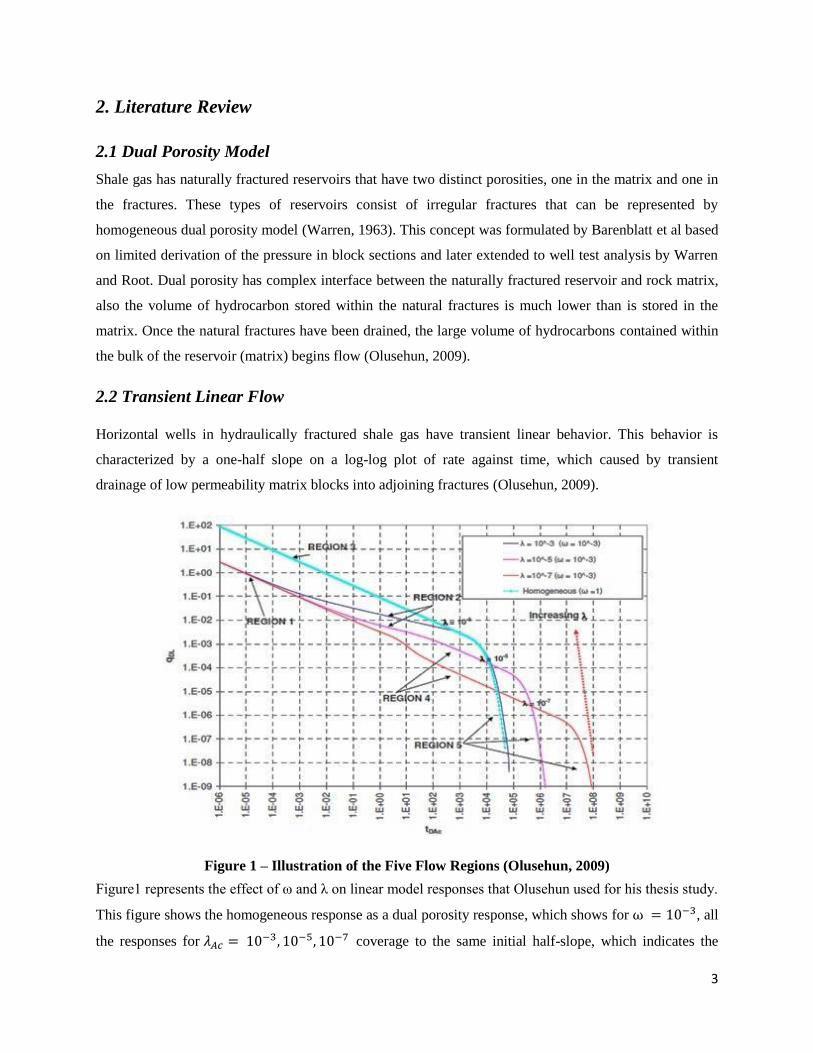
2.2 Transient Linear Flow

Horizontal wells in hydraulically fractured shale gas have transient linear behavior. This behavior is

characterized by a one-half slope on a log-log plot of rate against time, which caused by transient

drainage of low permeability matrix blocks into adjoining fractures (Olusehun, 2009).

Figure 1 – Illustration of the Five Flow Regions (Olusehun, 2009)

Figure1 represents the effect of ω and λ on linear model responses that Olusehun used for his thesis study.

This figure shows the homogeneous response as a dual porosity response, which shows for , all

the responses for coverage to the same initial half-slope, which indicates the

4

linear flow in the fractures, at early times and different half slopes at later times. The half slope at later

times is indicative of linear flow in the matrix. Region 1 represents early transient linear from in the

fracture, Region 2 represents bilinear flow caused by simultaneous transient flow in the fracture and

matrix that is indicated by a one-quarter slope on a log-log plot. Region 3 represents the homogeneous

reservoir; Region 4 represents the transient linear case, which is the purpose of the current study and

Region 5 that represents the period when the reservoir boundary. Using a one-half slope line on a log-log

plot can indicate region 3 and 4.

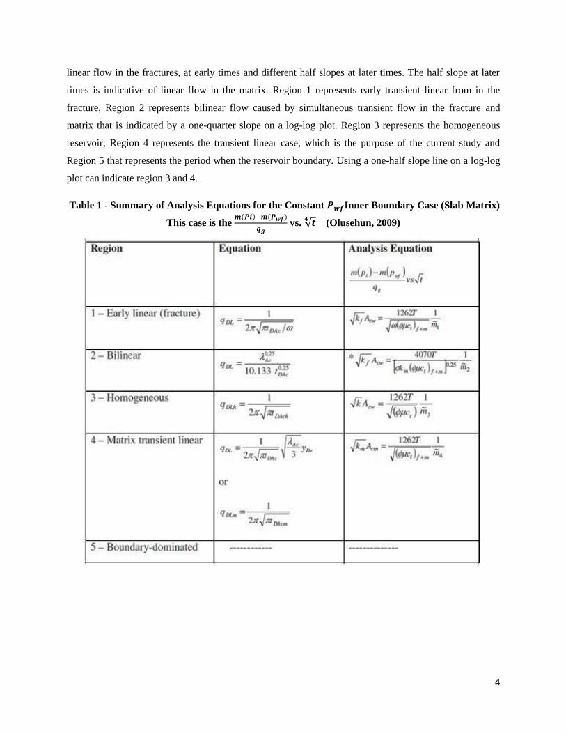
Table 1 - Summary of Analysis Equations for the Constant Inner Boundary Case (Slab Matrix)

This case is the

vs. √

(Olusehun, 2009)

5

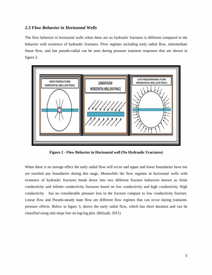
2.3 Flow Behavior in Horizontal Wells

The flow behavior in horizontal wells when there are no hydraulic fractures is different compared to the

behavior with existence of hydraulic fractures. Flow regimes including early radial flow, intermediate

linear flow, and late pseudo-radial can be seen during pressure transient responses that are shown in

figure 2.

Figure 2 - Flow Behavior in Horizontal well (No Hydraulic Fractures)

When there is no storage effect the early radial flow will occur and upper and lower boundaries have not

yet touched any boundaries during this stage. Meanwhile the flow regimes in horizontal wells with

existence of hydraulic fractures break down into two different fracture behaviors known as finite

conductivity and infinite conductivity fractures based on low conductivity and high conductivity High

conductivity has no considerable pressure loss in the fracture compare to low conductivity fracture.

Linear flow and Pseudo-steady state flow are different flow regimes that can occur during transient-

pressure effects. Below in figure 3, shows the early radial flow, which has short duration and can be

classified using unit slope line on log-log plot. (Belyadi, 2011)

6

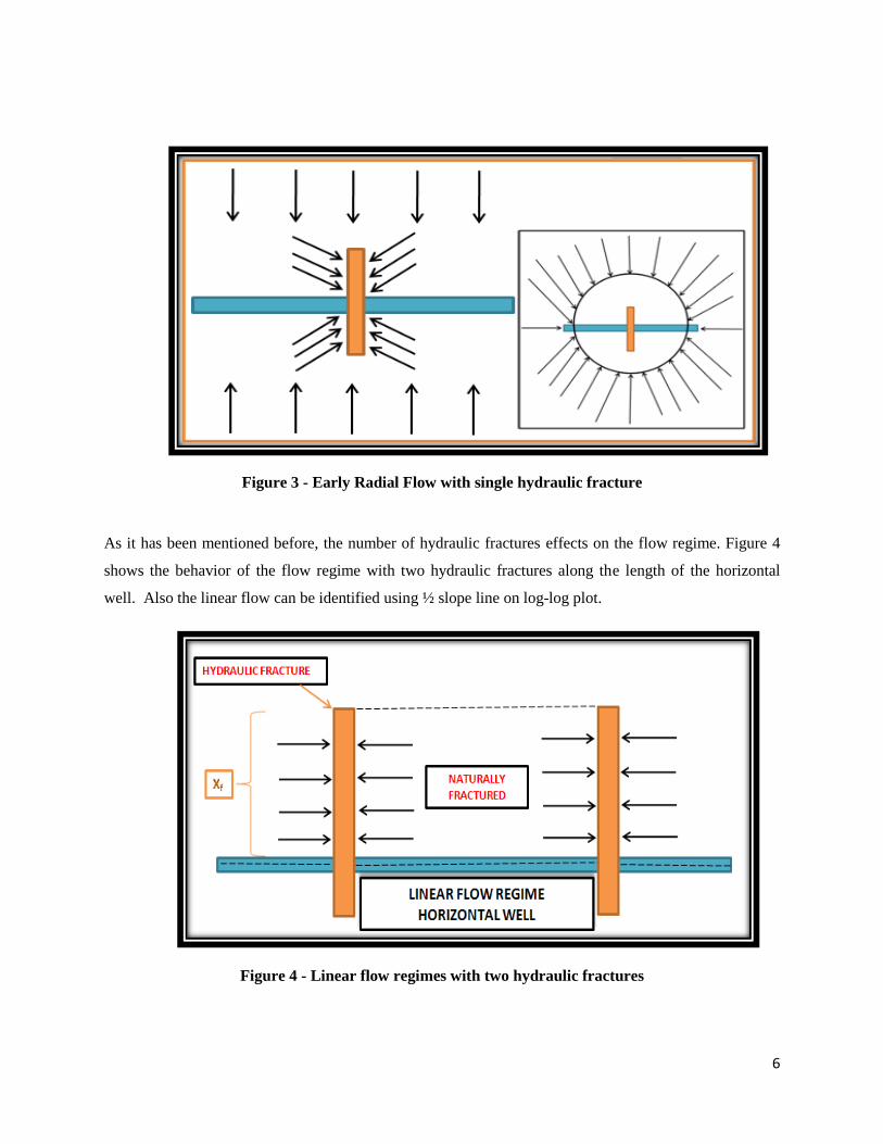
Figure 3 - Early Radial Flow with single hydraulic fracture

As it has been mentioned before, the number of hydraulic fractures effects on the flow regime. Figure 4

shows the behavior of the flow regime with two hydraulic fractures along the length of the horizontal

well. Also the linear flow can be identified using ½ slope line on log-log plot.

Figure 4 - Linear flow regimes with two hydraulic fractures

7

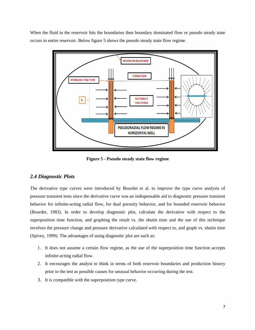
When the fluid in the reservoir hits the boundaries then boundary dominated flow or pseudo steady state

occurs in entire reservoir. Below figure 5 shows the pseudo steady state flow regime.

Figure 5 - Pseudo steady state flow regime

2.4 Diagnostic Plots

The derivative type curves were introduced by Bourdet et al. to improve the type curve analysis of

pressure transient tests since the derivative curve was an indispensable aid to diagnostic pressure transient

behavior for infinite-acting radial flow, for dual porosity behavior, and for bounded reservoir behavior

(Bourdet, 1983). In order to develop diagnostic plot, calculate the derivative with respect to the

superposition time function, and graphing the result vs. the shutin time and the use of this technique

involves the pressure change and pressure derivative calculated with respect to, and graph vs. shutin time

(Spivey, 1999). The advantages of using diagnostic plot are such as:

1. It does not assume a certain flow regime, as the use of the superposition time function accepts

infinite-acting radial flow.

2. It encourages the analyst to think in terms of both reservoir boundaries and production history

prior to the test as possible causes for unusual behavior occurring during the test.

3. It is compatible with the superposition type curve.

8

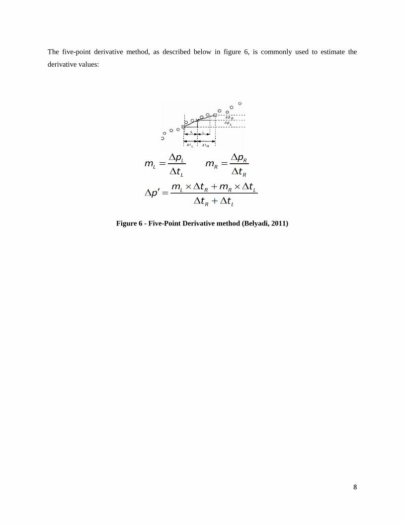
The five-point derivative method, as described below in figure 6, is commonly used to estimate the

derivative values:

Figure 6 - Five-Point Derivative method (Belyadi, 2011)

9

3. Objective and Methodology

3.1 Objective

The objective of this study is to understand the impacts of hydraulic fractures on flow behavior of the

horizontal wells completed in ultra-low permeability shale formations such as Marcellus Shale. A

commercial reservoir simulator has been employed to build a model with a horizontal well completed in

ultra-low permeability shale with several hydraulic fracture stages.

3. 2. Methodology

The methodology that was employed in this study consisted of the following steps:

1. Creating a base model to simulate production history for a horizontal well completed in ultra-low

permeability formation.

2. Identifying the various flow periods (regimes) associated with hydraulically fractured horizontal

wells using the diagnostic plots.

3. Investigating the impact of various shale characteristics on the duration of the flow periods.

3.2.1. Step 1.Simulation Base Model

A commercial reservoir simulator (ECLIPSE) was used to simulate 30-year production profile for a

horizontal well in ultra-low permeability shale. The simulated production rates were then used to generate

a diagnostic plot to determine the flow regimes. The base model consisted of a rectangular drainage area

4000 feet by 2000 feet containing a 3000-feet horizontal well.

The other important parameters for the model were established based on the available field information as

well as the results of the previous production history matching for Marcellus Shale wells (Belyadi, H.

2011) and are listed below in Table 2. A multi-layer, dual porosity model, which included adsorbed gas,

was employed to generate the production profiles. In addition, production profiles without adsorbed gas

were generated by setting the Langmuir Concentration to 0 MSCF/ton.

Tables 2 through 4 summarize other constant inputs and different properties for various numbers of

hydraulic fracture stages.

Table 3 illustrates the layers and rock properties that were used for the base model. There were total of

five layers in the model and top of the first layer is at 7000 feet. Each layer has a thickness of 15 feet.

Table 4 includes the hydraulic fractures’ properties. Four different cases were investigated, they are the

10

model with No hydraulic fractures, 1, 2, 4 hydraulic fracture stages. The hydraulic fracture stages were

placed as summarized in table 4 to have uniform spacing.

The grid-size in the model was chosen as 10 feet in all directions. The early production rates were found

to be significantly higher than the rest of the production profile. This problem is due to the fact that the

model treats the first grid block next to the wellbore as the hydraulic fracture. Consequently, the fracture

dimensions, in a model with large grid blocks, are significantly larger than the actual fracture dimensions.

This leads to over-prediction of the production rate at early times. To resolve this issue, the simulation

runs were performed using minimum grid sizes of 1 ft. in all directions. It should also mention that the

run-time for the model with small gird blocks was excessive. After comparing the new results to previous

results, it became clear that after 3 to 4 years of production, the simulated production rates were almost

identical for both runs. In order to have consistent results while reducing the run-time, the first 5 years of

the production was simulated using the model with smaller minimum grid size and the remainder of

production profile was obtained from the model with the larger minimum grid block size.

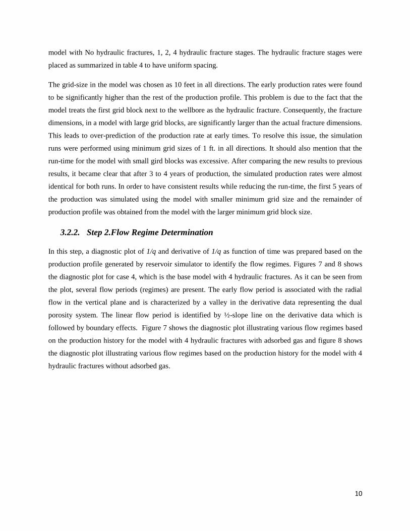
3.2.2. Step 2.Flow Regime Determination

In this step, a diagnostic plot of 1/q and derivative of 1/q as function of time was prepared based on the

production profile generated by reservoir simulator to identify the flow regimes. Figures 7 and 8 shows

the diagnostic plot for case 4, which is the base model with 4 hydraulic fractures. As it can be seen from

the plot, several flow periods (regimes) are present. The early flow period is associated with the radial

flow in the vertical plane and is characterized by a valley in the derivative data representing the dual

porosity system. The linear flow period is identified by ½-slope line on the derivative data which is

followed by boundary effects. Figure 7 shows the diagnostic plot illustrating various flow regimes based

on the production history for the model with 4 hydraulic fractures with adsorbed gas and figure 8 shows

the diagnostic plot illustrating various flow regimes based on the production history for the model with 4

hydraulic fractures without adsorbed gas.

11

Table 2 - Basic Model Parameters

Reservoir parameters

Depth, ft. 7,000

Thickness, ft. 75

Rock Properties

Fracture spacing, dimensionless 0.0073

Coal Compress, 1/psia 0.000001

Rock Density, Units 150

Fracture Porosity 0.002

Matrix Porosity, mD 0.05

Fissure Permeability x, y, z mD 0.002, 0.002, 0.0002

Matrix Permeability x, y, z mD 0.0004, 0.0004, 0.00004

Initial Conditions

Pressure, psia 3,000

Water Saturation, fraction 0.15

Hydraulic Fractures Properties

Half Length, ft. 500

Width, in 0.01

Top of Fracture, ft. 7,000

Bottom of Fracture, ft. 7,075

Permeability, mD 20,000

Porosity, fraction 0.1

Well Production Control

Bottom Hole Pressure, psia 500

Fluid Properties

Standard Pressure, psia 14.7

Standard Temperature, F 60

Reference Temperature, F 120

Desorption

Gas Diffusion Coefficient, Units 1

Sorption Time, day 62

Langmuir Pressure, psia 635

Langmuir Concentration, MSCF/ton 0.08899

12

Table 3 - Constant Inputs for layers and Rock properties

Total of 5 Layers Rock Properties

Top Depth, ft. Thickness,

ft.

Length of

Reservoir, ft.

Width of Reservoir,

ft.

Fracture

Porosity

Fissure Perm,

mD

Matrix Perm,

mD

7000 7060 15 4000 2000 0.002 0.002 0.0004

Table 4 - Properties for 4 Hydraulic Fractures

Fracture Name F1 F2 F3 F4

Half Length 500 ft. 500 ft. 500 ft. 500 ft.

Width 0.01 in 0.01 in 0.01 in 0.01 in

Top of Fracture 7000 ft. 7000 ft. 7000 ft. 7000 ft.

Bottom of Fracture 7075 ft. 7075 ft. 7075 ft. 7075 ft.

X Center 500 ft. 1500 ft. 2500 ft. 3500 ft.

Y Center 1000 ft. 1000 ft. 1000 ft. 1000 ft.

Permeability 20000 mD 20000 mD 20000 mD 20000 mD

Porosity 0.1 0.1 0.1 0.1

Figure 8 shows the diagnostic plot illustrating various flow regimes based on the production history for

the model with 4 hydraulic fractures without adsorbed gas.

3.2.3. Step 3.Sensitivity Analysis

To investigate the impact of various shale characteristics on the duration of the flow period, calculated

derivatives and diagnostic plots were used. After plotting each case and found the start and end point for

each flow rate, it was easy to see the behavior of each flow regime based on variable parameters. There

are 4 scenarios that are shown in Table 5. Also Table 6 to Table 9 listed below show the detail inputs for

each scenarios and variable parameters are shown in bold.

3.2.3.1 First Scenario

As it shows in table 5, the base model with no desorption for cases 2, 3, and 4 were run with 250 feet

half-length size for hydraulic fractures with actual fissure permeability (0.002). Table 6 is an example for

case 4 inputs.

3.2.3.2 Second Scenario

The base model with original half-length size (500 feet) was run with 0.001 fissure permeability for case

3 (base model with 2 hydraulic fractures) and case 4 (base model with 4 hydraulic fractures). Table 7 is an

example for case 4 inputs.

13

Figure 7 – Diagnostic Plot Illustrating Various Flow Regimes

3.2.3.3 Third Scenario




3.2.3.4 Fourth Scenario




0.00001

0.0001

0.001

0.01

0.1

1

0.001 0.01 0.1 1 10 100Years

Model with No Desorption

1/q

Derivative

Dual

Porosity

Effect

14

Figure 8 - Diagnostic Plot Illustrating Various Flow Regimes

0.00001

0.0001

0.001

0.01

0.1

1

0.001 0.01 0.1 1 10 100

Years

Model with Desorption

1/q

Derivative

Vertical

Radial

15

Table 5 - Variable Parameters for Each Case

Case studies Half Length Fissure Permeability

For cases 2,3, and 4 250 ft. 0.002

For case 3 and 4 500 ft. 0.001



Table 6 - Hydraulic Fractures' Properties for 4 Fractures

Fracture Name F1 F2 F3 F4

Half Length 250 ft 250 ft 250 ft 250 ft

Width 0.01 in 0.01 in 0.01 in 0.01 in

Top of Fracture 7000 ft 7000 ft 7000 ft 7000 ft

Bottom of Fracture 7075 ft 7075 ft 7075 ft 7075 ft

X Center 500 ft 1500 ft 2500 ft 3500 ft

Y Center 1000 ft 1000 ft 1000 ft 1000 ft

Permeability 20000 md 20000 md 20000 md 20000 md

Porosity 0.1 0.1 0.1 0.1

Table 7 - Inputs for layers and Rock properties


Top Depth,

ft Thickness,

ft

Length of

Reservoir, ft

Width of

Reservoir, ft

Fracture

Porosity

Fissure Perm,

mD

Matrix Perm,

mD

7000 7060 15 4000 2000 0.002 0.001 0.0001



Top Depth, ft Thickness,

ft

Length of

Reservoir, ft

Width of

Reservoir, ft

Fracture

Porosity

Fissure Perm,

mD

Matrix Perm,

mD

7000 7060 15 4000 2000 0.002 0.005 0.0005



Top Depth, ft Thickness,

ft

Length of

Reservoir, ft

Width of

Reservoir, ft

Fracture

Porosity

Fissure Perm,

mD

Matrix Perm,

mD

7000 7060 15 4000 2000 0.002 0.01 0.001

16

4. Results and Discussions

The following sections summarize the results of modeling and simulation studies as well as the

interpretation of the results for each scenario.

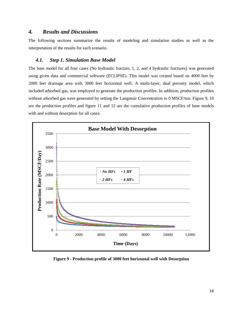
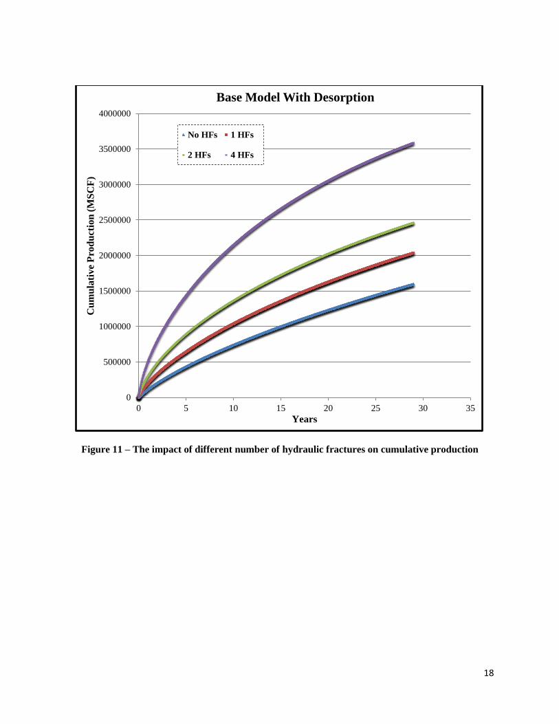
4.1. Step 1. Simulation Base Model

The base model for all four cases (No hydraulic fracture, 1, 2, and 4 hydraulic fractures) was generated

using given data and commercial software (ECLIPSE). This model was created based on 4000 feet by

2000 feet drainage area with 3000 feet horizontal well. A multi-layer, dual porosity model, which

included adsorbed gas, was employed to generate the production profiles. In addition, production profiles

without adsorbed gas were generated by setting the Langmuir Concentration to 0 MSCF/ton. Figure 9, 10

are the production profiles and figure 11 and 12 are the cumulative production profiles of base models

with and without desorption for all cases.

Figure 9 - Production profile of 3000 feet horizontal well with Desorption

0

500

1000

1500

2000

2500

3000

3500

0 2000 4000 6000 8000 10000 12000

Pro

du

ctio

n R

ate

(M

SC

F/D

ay)

Time (Days)

Base Model With Desorption

No HFs 1 HF

2 HFs 4 HFs

17

Figure 10 - Production profile of 3000 feet horizontal well with No Desorption

0

500

1000

1500

2000

2500

3000

3500

0 2000 4000 6000 8000 10000 12000

Pro

du

ctio

n R

ate

(M

SC

F/D

ay)

Time (Days)

Base Model With No Desorption

No HFs 1 HF

2 HFs 4 HFs

18

Figure 11 – The impact of different number of hydraulic fractures on cumulative production

0

500000

1000000

1500000

2000000

2500000

3000000

3500000

4000000

0 5 10 15 20 25 30 35

Cu

mu

lati

ve

Pro

du

ctio

n (

MS

CF

)

Years

Base Model With Desorption

No HFs 1 HFs

2 HFs 4 HFs

19

Figure 12 - The impact of different number of hydraulic fractures on cumulative production

0

500000

1000000

1500000

2000000

2500000

3000000

3500000

0 5 10 15 20 25 30 35

Cu

mu

lati

ve

Pro

du

ctio

n (

MS

CF

)

Years

Base Model With No Desorption

No HFs 1 HFs

2 HFs 4 HFs

20

4.2. Step 2. Flow Regime Determination

To determine the flow regimes, the derivative of production rate has been calculated and the diagnostic

plots were used to show the flow regime for each individual case with 3000 feet of horizontal lateral and

4000 by 2000 ft2 drainage area. Figures 13and 14 are diagnostic plots that shows all case studies together

and illustrates flow regimes for the case study with 1, 2, and 4 hydraulic fractures with base model using

diagnostic plots. The results include dual porosity effect and the flow is followed by linear flow and

compounded linear flow. Duration period is based on the drainage geometry as it shows in listed figures.

Figure 13 - Diagnostic plot showing flow periods for all 4 cases

0.00001

0.0001

0.001

0.01

0.001 0.01 0.1 1 10 100

Der

ivati

ves

Years

Base Model with Desorption

1 HF 2 HFs 4 HFs

Dual Porosity

Effect

21

Figure 14 - Diagnostic plot showing flow periods for all 4 cases

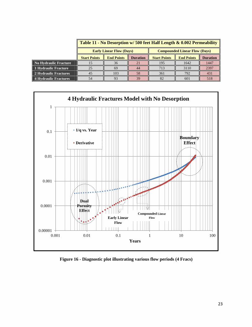
Figures 15 and 16 are representing the base model with 4 hydraulic fractures with and with no desorption

conditions. The properties for the base model are such as: permeability of 0.002 mD with 500 feet half-

length for hydraulic fractures and tables10 and 11 indicating the results for all cases. Below figures are

diagnostic plots presenting the flow durations for each condition. The duration period for early linear flow

for the model with 4 hydraulic fractures with desorption is 166 days and for the case when there is no

desorption goes up to 322 days of early linear flow. Also the flow duration for compounded linear flow

for desorption case travels up to 406 days and when there is no desorption, the duration flow is up to 174

days. The diagnostic plots for flow durations for models with 1 and 2 hydraulic fractures are included in

appendices.

0.00001

0.0001

0.001

0.01

0.1

1

0.001 0.01 0.1 1 10 100

Der

ivati

ves

Years

Base Model with No Desorption

1 HFs 2 HFs 4 HFs

Dual

Porosity

Effect

22

Table 10 -Desorption w/ 500 feet Half Length & 0.002 Permeability

Early Linear Flow (Days) Compounded Linear Flow (Days)

Start Points End Points Duration Start Points End Points Duration

No Hydraulic Fracture 15 36 21 205 3986 3782

1 Hydraulic Fracture 35 78 43 455 3150 2695

2 Hydraulic Fractures 45 136 91 414 908 495


Figure 15 - Diagnostic plot illustrating various flow periods (4 Fracs)

0.00001

0.0001

0.001

0.01

0.1

1

0.001 0.01 0.1 1 10 100Years

4 Hydraulic Fractures Model with Desorption

1/q vs. Year

Derivative

Compounded

Linear Flow

Boundary

Effect

Dual

Porosity

Effect

Early Linear

Flow

23

Table 11 - No Desorption w/ 500 feet Half Length & 0.002 Permeability



No Hydraulic Fracture 15 36 21 195 1642 1447




Figure 16 - Diagnostic plot illustrating various flow periods (4 Fracs)

0.00001

0.0001

0.001

0.01

0.1

1

0.001 0.01 0.1 1 10 100

Years

4 Hydraulic Fractures Model with No Desorption

1/q vs. Year

Derivative

Dual

Porosity

Effect

Boundary

Effect

Early Linear

Flow

Compounded Linear

Flow

24

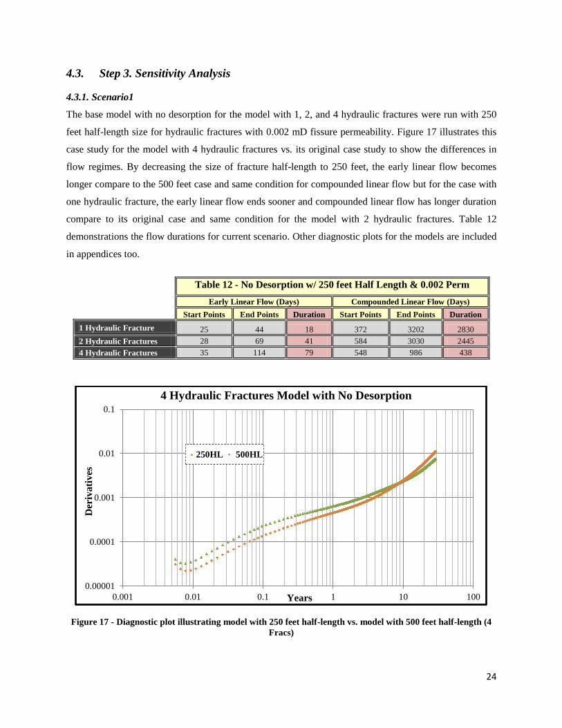
4.3. Step 3. Sensitivity Analysis

4.3.1. Scenario1

The base model with no desorption for the model with 1, 2, and 4 hydraulic fractures were run with 250

feet half-length size for hydraulic fractures with 0.002 mD fissure permeability. Figure 17 illustrates this

case study for the model with 4 hydraulic fractures vs. its original case study to show the differences in

flow regimes. By decreasing the size of fracture half-length to 250 feet, the early linear flow becomes

longer compare to the 500 feet case and same condition for compounded linear flow but for the case with

one hydraulic fracture, the early linear flow ends sooner and compounded linear flow has longer duration

compare to its original case and same condition for the model with 2 hydraulic fractures. Table 12

demonstrations the flow durations for current scenario. Other diagnostic plots for the models are included

in appendices too.

Figure 17 - Diagnostic plot illustrating model with 250 feet half-length vs. model with 500 feet half-length (4

Fracs)

0.00001

0.0001

0.001

0.01

0.1

0.001 0.01 0.1 1 10 100

Der

ivati

ves

Years


250HL 500HL

Table 12 - No Desorption w/ 250 feet Half Length & 0.002 Perm






25

4.3.2. Scenario2

The base model with no desorption for cases with 2 and 4 hydraulic fractures were run with 500 feet half-

length size of hydraulic fractures and 0.001 mD fissure permeability. Figure 18 illustrates this case study

for the model with 4 hydraulic fractures vs. its original case study to show the differences in flow

regimes. By decreasing the fissure permeability to 0.001 mD, the early and compounded linear flows will

have longer duration compare to the original case study. Table 13 shows the flow durations for both new

scenarios. Also a diagnostic plot for the model with 2 hydraulic fractures is included in appendix as well.

Table 13 - No Desorption Model w/ 500 feet Half Length and 0.001 Perm





Figure 18 - Diagnostic plot to show model for 4 hydraulic fractures w/ 0.001 permeability

0.00001

0.0001

0.001

0.01

0.1

0.001 0.01 0.1 1 10 100

Der

ivati

ves

Years


4HFs W/ 0.001 Perm

4HFs W/ 0.002 Perm

26

4.3.3. Scenario 3 and 4

The base model with no desorption for cases 3 and 4 were run with 500 feet half-length size for hydraulic

fractures with 0.005 mD fissure permeability for scenario 3, and 0.01 mD fissure permeability for

scenario 4. Figure 19 and 20 illustrates these two scenarios vs. their original case studies to show the

differences in flow regimes. Table 14 shows the flow durations for both new scenarios. Also a diagnostic

plot for case 3 is included in appendices section. By increasing the fissure permeability to 0.005 mD, the

linear flow for both scenarios flows longer period but for the scenario with 0.01 mD fissure permeability,

the linear flow becomes shorter and smaller duration periods.

Table 14 -No Desorption Model w/ 500 feet Half Length

With 0.005 Perm With 0.01 Perm





0.00001

0.0001

0.001

0.01

0.1

0.001 0.01 0.1 1 10 100

Der

ivati

ves

Years


4HFs W/ 0.002 Perm

4HFs W/ 0.005 Perm

27


0.000001

0.00001

0.0001

0.001

0.01

0.1

0.001 0.01 0.1 1 10 100

Der

iva

tiv

es

Years


4HFs W/ 0.002 Perm

4HFs W/ 0.01 Perm

28

5. Conclusions

The objective of this thesis was to understand the impacts of hydraulic fractures on flow behavior of the

horizontal wells completed in ultra-low permeability shale formations such as Marcellus Shale. After

creating the model and analyzed multiple cases, it was concluded that the number of hydraulic fractures

significantly impacts the production. Meanwhile the impact of desorption was found to be negligible

during the early stage of the production. This study identified a number of different flow regimes. The

first flow period identified was vertical radial flow that was influenced by the dual porosity effects. The

second flow period was “Early Linear Flow” which its duration depended on the number of hydraulic

fractures. The next flow period identified was “Compounded Linear Flow” which its duration also

depended on the number of hydraulic fractures. Finally, the flow becomes elliptical due to boundary

effects.

The detail investigation of the flow regimes revealed that as the number of hydraulic fracture increases,

the duration of the “Early Linear Flow” becomes longer. However, as the number of hydraulic fracture

increases, the duration of the “Compounded Linear Flow” becomes shorter. This is because the boundary

effects occur earlier with the increase in the number of hydraulic fracture. The fracture half-length also

impacts the flow periods. The shore the fracture half-length, the shorter is the “Early Linear Flow” and

the longer is the “Compounded Linear Flow. Also fissure permeability is another parameter that had

major impact on the flow periods. The study showed that as the fissure permeability increases, the linear

flow diminishes because the transient period becomes shorter.

29

6. Recommendations for future work

A case with more horizontal wells with multiples clusters of hydraulic fractures can be investigated for

the flow regimes identifications. Moreover, a real case can be used to apply the developed workflow for

identifying different flow regimes.

30

References

1. Anon., 2013. Shale gas in the United States. [Online]

Available at: http://en.wikipedia.org

[Accessed 19 May 2013].

2. Barenblatt, 1960. Basic concepts in the theory of homogeneous liquids in fissure rocks, s.l.: s.n.

3. Belyadi, A., 2010. Performance of the Hydraulically Fractured Horizontal Wells in Low

Permeability Formation. s.l., Society of Petroleum Engineers Inc. SPE139082.

4. Belyadi, A., 2011. Modeling Studies To Evaluate Performance of the Horizontal Wells Completed

in shale, Morgantown: West Virginia.

5. Belyadi, A., 2012. Production Performance of Mulityply Fractured Horizontal Wells.

Morgantown, SPE.

6. Bourdet, D. e. a., 1983. A new set of type curves simplifies well test analysis. s.l.:s.n.

7. Gringarten, A. C., n.d. Type-Curve Analysis. s.l., Society of Petroleum Engineers Inc. .

8. Kalantari, A., 2010. Reservoir Modeling of New Albany Shale , Morgantown: s.n.

9. Olusehun, R., 2009. Rate Transient Analysis in Shale Gas Reservoirs with Transient Linear

Behavior, College Station, TX: s.n.

10. Spivey, J. P., 1999. Application of the Diagnostic plot using a Derivative Based on Shut-In Time.

s.l., Society of Petroleum Engineers Inc. SPE 56424..

11. Warren, 1963. The Behavior of Naturally Fractured Reservoirs. s.l., Society of Petroleum

Engineers.

31

Appendices

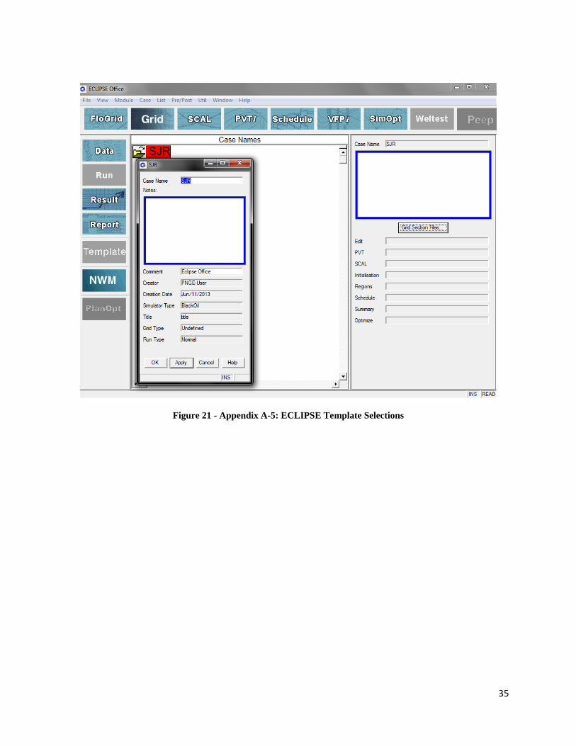
Appendix A (ECLIPSE)

Appendix A-1 shows simple procedure using Schlumberger ECLIPSE software to model horizontal well

completed in shale. Step by step of this procedure is included. Figure A-1 shows an Eclipse software

launcher screen that was used in this research.

Figure 17 - Appendix A-1: ECLIPSE Launcher

32

Before choosing of any options excited in the launcher, create a file for the model that needs to becreated,

then click on the office tab from the software launcher window to select the file that has been created and

run the launcher. Figure 18 is an example of what was explained.

Figure 18 - Appendix A-2: ECLIPSE Office Launcher

33

Figure 19 shows the next step, which is creating a project. Click on file and there click on the “New

Project” option.

Figure 19 - Appendix A-3: ECLIPSE Office Screen

34

After creating the project, click on the “Add Template Case” option as it shown in figure 20. Then the

template selection panel will be displayed as it shows in figures 21 and 22. The user will be able to select

the detail of the model.

Figure 20 – Appendix A-4: ECLIPSE Template Screen

35

Figure 21 - Appendix A-5: ECLIPSE Template Selections

36

Figure 22 - Appendix A-6: ECLIPSE Template Screen

37

After creating the template for the model, click on to move on to the next step of the creating the model.

Figure 23 shows the Model Definition window, which has the start and end day, month, and year, also

model properties. The user selects and enters the workflow is shown in this figure.

Figure 23 - Appendix A-7: Model Definition

The next step is the “Reservoir Description”, which this section has its own work flow to follow. Figure

24 displays the window for layer information, which includes layer name, top depths, thickness, Length

and width for each layer.

Figure 24 - Appendix A-8: Reservoir Layers Description

38

Figure 25 displays the “Rock Properties” window, which is the next work flow in “Reservoir

Description”. Rock properties contain rock name, fracture porosity, fissure permeability, matrix porosity

and so on that shows in listed figure.

Figure 25 - Appendix A-9: Rock Properties

Next step in Reservoir Description is the “Non-Equilibrium Initial Conditions”, which the user enters the

reservoir pressure and water saturation for the model.

Figure 26 - Appendix A-10: Non-Equilibrium Initial Conditions

39

For this study, the aquifers data wasn’t used. The last step of the reservoir description is the “Fractures”

data entry. Figure 27 shows the detail of this work.

Figure 27 - Appendix A-11: Fractures

Continuing the next work flow is the access to well location in terms of its deviation survey data

coordinates. Figure 28 shows the detail of this work flow to enter either horizontal or vertical wells for

the model.

Figure 28 - Appendix A-12: Well Control

At this point, the user is fully done with 3 steps and following steps starts off with production tab. In this

step, new even from available event types needs to be selected and the user can click on the “Production

40

Well Schedule Data”. Continue selecting well controls tab and enter the information related to start date,

control mode, open/shut flag and target pressure. Figure 29 shows listed stages also figure 30 shows the

user to define the perforation from the event type’ drop-down box.

Figure 29 - Appendix A-13: Production Well Control

Figure 30 - Appendix A-14: Perforation Control

Figures 31to 34 illustrates the work flow for the “Fluid Properties” for the model. At this stage, the

information for PVT Composition, Rel. Perm, and Coal Bed Methane are used.

41

Figure 31 - Appendix A-15: PVT Composition

Figure 32 - Appendix A-16: Rel. Perm for Gas

42

Figure 33 - Appendix A-17: Rel. Perm for Water

Figure 34 - Appendix A-17: Coal Bed Methane

43

The last work flow that was used to complete this model is the “Simulation Control for Gridding

Control”. Figures 35 and 36 illustrate the details for gridding and turning controls. The minimum and

maximum cell sizes needs to be determined by the user, also cell per layers in the gridding control data.

Meanwhile, turning controls was used for time-step, minimum time-step, maximum time-step, maximum

pressure change per time-step, maximum non-linear iteration, and maximum linear iteration data entry.

Figure 35 - Appendix A-18: Simulation Controls for Gridding Controls

Figure 36 - Appendix A-19: Simulation Controls for Turning Controls

At this point, the user has completed data entry to build the model and by clicking on generating model,

then run ECLIPSE, and at the end view results will be able to achieve the results.

44

Appendix B (ECLIPSE Models Layouts)

Figure 37 - Appendix B-1: Model with 1 Hydraulic Fracture

Figure 38 - Appendix B-2: Model with 2 Hydraulic Fractures

Figure 39 - Appendix B-3: Model with 4 Hydraulic Fractures

45

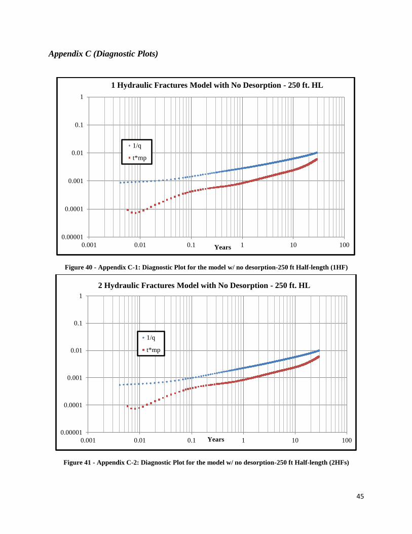
Appendix C (Diagnostic Plots)

Figure 40 - Appendix C-1: Diagnostic Plot for the model w/ no desorption-250 ft Half-length (1HF)

Figure 41 - Appendix C-2: Diagnostic Plot for the model w/ no desorption-250 ft Half-length (2HFs)

0.00001

0.0001

0.001

0.01

0.1

1

0.001 0.01 0.1 1 10 100Years

1 Hydraulic Fractures Model with No Desorption - 250 ft. HL

1/q

t*mp

0.00001

0.0001

0.001

0.01

0.1

1

0.001 0.01 0.1 1 10 100Years


1/q

t*mp

46

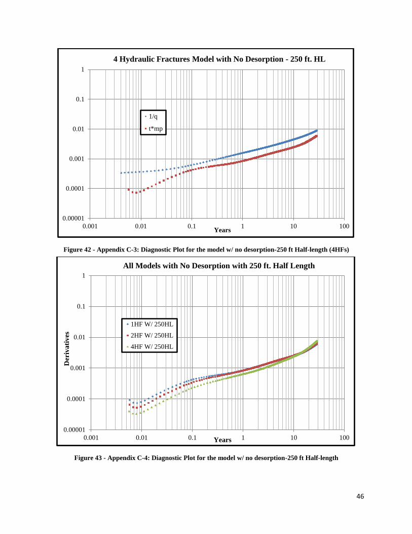
Figure 42 - Appendix C-3: Diagnostic Plot for the model w/ no desorption-250 ft Half-length (4HFs)

Figure 43 - Appendix C-4: Diagnostic Plot for the model w/ no desorption-250 ft Half-length

0.00001

0.0001

0.001

0.01

0.1

1

0.001 0.01 0.1 1 10 100Years


1/q

t*mp

0.00001

0.0001

0.001

0.01

0.1

1

0.001 0.01 0.1 1 10 100

Der

ivati

ves

Years

All Models with No Desorption with 250 ft. Half Length

1HF W/ 250HL

2HF W/ 250HL

4HF W/ 250HL

47

Figure 44 - Appendix C-5: Diagnostic plot for model for 2 hydraulic fractures w/ 0.001 permeability


0.00001

0.0001

0.001

0.01

0.1

0.001 0.01 0.1 1 10 100Years

Model with 2 Fracs w/ No Desorption - 0.001 Permeability

1/q vs. Year

Derivative

0.00001

0.0001

0.001

0.01

0.1

0.001 0.01 0.1 1 10 100Years

Model with 2Hydraulic Fractures - 0.005 Permeability

1/q vs. Year

Derivative

48


Figure 47 - Appendix C-8: Diagnostic plots for all scenarios for model with 2 hydraulic fractures

0.00001

0.0001

0.001

0.01

0.1

0.001 0.01 0.1 1 10 100Years

Model with 2Hydraulic Fractures - 0.01 Permeability

1/q vs. Year

Derivative

0.00001

0.0001

0.001

0.01

0.1

0.001 0.01 0.1 1 10 100Years

Derivatives

2HFs W/ 0.001 Perm

2HFs W/ 0.002 Perm

2HFs W/ 0.005 Perm

2HFs W/ 0.01 Perm

49

Figure 48 - Appendix C-9: Diagnostic plots for all scenarios for model with 4 hydraulic fractures

0.000001

0.00001

0.0001

0.001

0.01

0.1

0.001 0.01 0.1 1 10 100Years

Derivatives

4HFs W/ 0.001 Perm

4HFs W/ 0.002 Perm

4HFs W/ 0.005 Perm

4HFs W/ 0.01 Perm

Date post:	13-Mar-2022
Category:	Documents
Upload:	others
View:	6 times
Download:	0 times

The Flow Regimes Associated with Hydraulic Fractured ...

Documents