AAS 03-274

The Flower Constellations

Daniele Mortari∗, Matthew P. Wilkins†, and Christian Bruccoleri‡

Department of Aerospace Engineering,Texas A&M University, College Station, TX 77843-3141

Abstract

This paper defines a set of satellite constellations, called the Flower Con-stellation Set, that generalize the multi-stationary inclined orbits having re-peatable ground tracks. With various satellite phasing schemes, Flower Con-stellations present many interesting features useful for telecommunication,deep space observation, global positioning systems, and formation flying. AFlower Constellation, which can be symmetric or asymmetric, is defined bysix independent parameters: the number of petals (Np), the number of side-real days to repeat the ground track (Nd), the number of satellites (Ns), theargument of perigee (ω), the orbit critical inclination (i), and the perigeealtitude (hp). Thus, in specific, we will refer to a particular constellation asa Np-Nd-Ns-ω-i-hp Flower Constellation but, in general, we will use simplya Np-Nd Flower Constellation. It is shown that some of the proposed pastsatellite constellations, as for instance the 1967 Broglio’s Sistema Quadri-foglio, are specific Flower Constellation cases. Some specific Flower Constel-lations are described and discussed in detail to demonstrate some potentialapplications.

1 Introduction

In this paper, we consider constellations of satellites all having the same repeatingground track. That is to say, no matter how many satellites are considered for the

∗Associate Professor, Department of Aerospace Engineering, 741A H.R. Bright Building, TexasA&M University, 3141 TAMU, College Station, Texas 77843-3141. Tel. (979) 845-0734, FAX (979)845-6051. AIAA and AAS Member.

†Graduate Research Assistant, Aerospace Engineering Department, 631B H.R. Bright Build-ing, Texas A&M University, 3141 TAMU, College Station, Texas 77843-3141 Tel. (979) 845-0745,mwilkins@tamu.edu. AIAA and AAS Member.

‡Graduate Research Assistant, Department of Aerospace Engineering, 620C H.R. Bright Building,Texas A&M University, College Station, TX 77843-3141, Tel. (979) 458-0550, bruccoleri@tamu.edu

1

constellation, from an Earth Centered Fixed (ECF) reference frame (i.e. a framerotating with the Earth), they all follow a single ground track. The concept of repeatground track constellations has been around for a number of years. Thus, we startoff with a brief survey of those constellations on the way to the generalization of theFlower Constellation.

1.1 Survey of the satellite constellations

Dating back to 1967, first reported in 1981 as part of the University of Rome/NASASan Marco Project, the Four-Leaf Clover System (Sistema Quadrifoglio)[1] is a con-stellation of four satellites, whose orbital parameters are given in Table 1 where T , Ω,

Satellite T Ω + ω i M0

#1 Ts/3 0 0 0#2 Ts/3 π/2 0 π/2#3 Ts/3 π 0 π#4 Ts/3 3π/2 0 3π/2

Table 1: The Four-Leaf Clover System

ω, i, and M0 represent the orbital period, the right ascension of the ascending node,the argument of perigee, the inclination, and the mean anomaly at the initial time,respectively. Ts is the sidereal rotation rate of the Earth.

This constellation was originally proposed to observe and to guarantee continuousmeasurement of the upper part of the atmosphere in the equatorial region. The pur-pose was to find out the relationships between the physical properties of the equatorialtroposphere with the Solar and Geomagnetic activities.

The beauty of the dynamics of this constellation can be best appreciated in an ECFsystem of coordinates. The satellites each spend about six hours near apogee and twohours in transition between successive apogees. Due to the phasing of the satellites inthe orbits, three of the satellites are always near apogee and the other is in transitionto replace the spacecraft with the largest mean anomaly (the one about to movequickly toward perigee). Finally, the three spacecraft near apogee (about 120 apart)have line of sight visibility of each other and each can observe well over 1/3 of theEarth’s surface. The idea of this constellation is quite old, but there exists onlyone published paper on it (see Ref. [2]). This paper mainly analyzed the timehistory of the orbital parameters, and suggested that the perigee altitude be raisedto hp = 600 km in order to reduce the atmospheric drag.

Since that time, a number of new constellation concepts similar in nature to theClover have been developed. These constellations are based upon the many categoriesof satellite orbits that exist today: Low Earth Orbits (LEO), Molniya [a subset of

2

Parameters Molinya Tundra LoopusPeriod [h] 12 24 14.4

Eccentricity 0.65 0.2 0.6Apogee height [km] 39400 44220 41700Perigee height [km] 2900 27350 5642

Table 2: Parameters of HEO orbits.

Highly Eccentric Orbits (HEO)], TUNDRA orbits, Geosynchronous/GeostationaryEarth Orbits (GEO), Intermediate Circular Orbits (ICO), APTS (Apogee AlwaysPointing to the Sun) orbits[3, 4], and Multistationary Inclined Orbits (MIO). A num-ber of the pertinent constellation concepts are: Walker Constellations, Beste Con-stellations, the “Gear array”[5], Ellipso[6], Multi-regional Highly Eccentric Orbits(M-HEO)[7], Juggler Orbit COnStellation (JOCOS)[8], Loops in Orbit Occupied Per-manently by Un-stationary Satellites (LOOPUS)[9], SYstem COmmunication MO-bile RElayed Satellite (SYCOMORES) [10], UK T-SAT[11], and CommunicationsOrbiting Broadband Repeating Arrays (COBRA)[12]. Apparently, no one has yetundertaken a generalization of these types of constellations.

These constellations have generated considerable interest in the telecommunicationsindustries (especially in the European countries) for their ability to address certainspecific needs, namely global and regional telecommunications coverage[13, 14]. Tothat end, the European Space Agency commissioned a study called Archimedes be-ginning in the late 80’s and early 90’s[15], which included the major space agenciesin Western and Eastern Europe. This study searched for a constellation conceptthat would improve the poor reception from GEO satellites at higher latitudes. Forinstance, due to the low grazing angle between a point on the ground and a GEOsatellite, buildings, terrain, and even trees often would disrupt cell phone use in Eu-rope making it difficult to provide continuous service to users. The Archimedes effortstudied many of the aforementioned constellation concepts and settled upon two ba-sic designs based upon the Molniya (12 hour period) and TUNDRA (24 hour period)orbits.

Besides the Sistema Quadrifoglio, of particular interest are the HEO and MIO con-stellation concepts. Within these categories, the JOCOS, LOOPUS, and COBRAconcepts have the most bearing, and we will consider the relative merits of theseconstellations. A brief description of these concepts are given below.

1.1.1 HEO/MIO

Highly Eccentric Orbit constellations typically have a perigee altitude at or above 500Km and apogee altitudes can be in excess of 7 Earth radii (refer to Table 2). Often,as in the case of the Molinya orbits, the orbits are inclined at 63.4 or 116.6 in order

3

to minimize the movement of the line of apsides and reduce orbit maintenance costs.Additionally, due to the high eccentricity of these orbits, an individual satellite willspend about two thirds of the orbital period near apogee, and, during that time, itappears to be almost stationary for an observer on the earth (this is often referred toas apogee dwell).

Multistationary Inclined Orbit constellations are extensions of HEO constellations inthat they generally refer to orbits which have repeating ground tracks. This, combinedwith the long apogee dwell time, create constellations where satellites spend up totwo-thirds of their time over a particular region of the Earth.

1.1.2 JOCOS

The JOCOS concept involves the use of 8 hr, circular, inclined, repeating orbits.In that regard, the apogee location becomes irrelevant, and an orbit inclination of75 was chosen to maximize Earth coverage. Six satellites are placed in orbits withnodes evenly arrayed. The mean anomalies of the satellites are chosen such that threesatellites will be in the northern hemisphere and three will be in the southern. Asthe top 3 simultaneously descend, the bottom 3 will simultaneously ascend to replacethem. Thus, continued coverage of the Earth is assured. However, this particulardesign leaves gaps at the highest points of the orbits during the exchange, and anextra satellite must be placed into the mix to ensure complete coverage. For thisreason, you will often see JOCOS referred to as the 6+1 JOCOS constellation. TheJOCOS constellation is so named because it “juggles” 3 + 3 satellites simultaneouslywith three up and three down at any given time.

1.1.3 LOOPUS

LOOPUS (quasi-geostationary Loops in Orbit Occupied Permanently by Unstation-ary Satellites)is a constellation constructed from circular or HEO orbits. The LOO-PUS concept focuses on solutions where loops are formed in the ground track. Thesatellites are arrayed such that two satellites will reach the intersection of the loop(one entering and one leaving) almost simultaneously where a communications hand-over is performed. As defined by Peter Dondl in 1984, the following parametersdescribe a LOOPUS system: n, the number of LOOPUS positions; m, the number ofsatellites; To, the satellite orbit period; and Td, the dwelling time interval.

In general, for the non-circular orbits, the orbital inclination is chosen to be thecritical inclination of 63.4. Thus, assuming values of n = 2, m = 3, T0 = 12 hrand Td = 8 hr, the LOOPUS concept will create a system of satellites which are in aMolinya orbit and have equally spaced nodes 120 apart. The name LOOPUS comesfrom the fact that the ground track creates a loop at apogee where the satellites spendup to two thirds of their time.

4

1.1.4 COBRA

The COBRA Teardrop concept involves two MIOs where the argument of perigeeis not 90 or 270, which would normally ensure that the location of the apogees isalways over the southern or northern hemispheres, respectively. By choosing othervalues for the argument of perigee, a “lean” is created in the ground track. Bycombining two repeat track orbits, one with a right “lean” and the other with aleft “lean”, a “teardrop” intersection is created. As in the LOOPUS concept, theintersection points are used to hand over communications responsibilities betweensatellites in the constellation.

2 Theory of the Flower Constellation Set

We propose to unify the Four-Leaf Clover System and other specific constellationtypes by introducing the Flower Constellation Set, which is constituted by critically-inclined, compatible orbits. Generally, all the orbits in a given Flower Constellationare:

• Identically inclined at one of the critical inclinations: i = 63.4, or i = 116.6,which implies ω = 0. That is, without a significant control effort being applied,no rotation of the apsidal line is permissible because it would eventually disruptthe constellation.

• Compatible: the orbital period is evaluated in such a way as to yield a per-fectly repeated ground track. That is, perturbations such as the J2 effect areincorporated through the inclusion of time rates of change of the orbit elements.

• For an axial-symmetric Flower Constellation, the node lines of each satelliteare equally displaced along the equatorial plane. Non-axial-symmetric FlowerConstellations have satellites with RAANs that are integer multiples of eachother.

Because of the resulting orbit path in the relative frame resembles the outlines of aflower petal, this set of constellations is called the Flower Constellation Set. Hereafter,we present the basic concepts that demonstrate how this set of constellations can begenerated.

2.1 Repeating Ground Tracks

To begin, an orbit can be designed such that its ground track will repeat after onecomplete orbit around the Earth. Ideally, all that needs to be ensured is that thenodal period of the orbit, TΩ, precisely matches the nodal period of Greenwich, TΩG.

5

Not only can we set the nodal periods equal, but also we can extend this concept toa ground track that will repeat after the satellite completes Np revolutions over Nd

days. If Tr is the period of repetition, then

Tr = Np TΩ = Nd TΩG (1)

Here, we note that the value of Np, indicating the number of revolutions required tocomplete one period of repetition, corresponds to the number of “petals” that appearabout the Earth in the ECF frame. Because of the petal-like shape of the orbits whenviewed from a relative frame, we refer to a constellation of satellites which all havethe exact same repeating ground track as a Flower Constellation.

We will need to determine a relationship between the nodal period, TΩ, and theanomalistic period (i.e. perigee to perigee), T . Once the anomalistic period of theorbit has been established, we can then determine the semi-major axis, a. The ec-centricity, e, of the orbit can be determined from a and a specified perigee altitude.Once the semi-major axis and eccentricity have been defined, the shape of the orbitis completely determined, and all that remains is to specify its orientation in space.

2.2 Finding the Nodal Period

We begin our discussion by examining the nodal period equations. Carter defines thenodal period of Greenwich as:[16]

TΩG =2π

ω⊕ − Ω(2)

where ω⊕ is the rotation rate of the Earth given by

ω⊕ = 7.29211585530× 10−5 rad/s (3)

and Ω is the nodal regression of a satellite’s orbit plane caused by perturbations suchas the Earth’s oblateness. Because we are only considering orbits which repeat overa small fraction of a year, we will generally ignore the nodal regression of Greenwichdue to luni-solar effects.

Following the development presented in Vallado, we can also determine the nodalperiod of the satellite as a function of its anomalistic period, T , as follows:[17]

TΩ =2π

M + ω=

2π

n + M0 + ω=

2π

n

(1 +

M0 + ω

n

)−1

= T

(1 +

M0 + ω

n

)−1

(4)

where n is the satellite’s mean motion, M0 is the rate of change in the mean anomalydue to perturbations, and ω is the rate of change in the argument of perigee due toperturbations.

6

0 20 40 60 80 100 120 140 160 180−0.6

−0.4

−0.2

0

0.2

0.4

0.6

0.8

1

1.2

Np = 3, N

d = 1, T = 7.9781 hr, h

p = 600 Km, h

a = 33562.6743 Km.

Inclination (deg)

Rat

e of

cha

nge

(deg

/day

)

ω

M

Ω

Figure 1: Rate of change for a given Flower Constellation

We can find expressions for M0, ω, and Ω from geopotential perturbation theory. If weonly consider second order zonal effects, then the following expressions are valid:[17]

ω = ξ n (4− 5 sin2 i)

Ω = −2 ξ n cos i

M0 = −ξ n√

1− e2 (3 sin2 i− 2)

where ξ =3R2

⊕J2

4p2(5)

where R⊕ = 6, 378.1363 Km is the mean radius of the Earth, J2 = 1.0826269× 10−3,p is the orbit semi-parameter, and i is the orbit inclination.

Vallado continues on by assuming circular orbits (i.e. e ≈ 0). However, generally, ourorbits under consideration will be highly elliptic. Thus, the following developmentkeeps the eccentricity terms. By substituting Equation 5 into Equation 4 and withsome algebraic manipulation, we obtain:

TΩ = T

1 + ξ[4 + 2

√1− e2 − (5 + 3

√1− e2) sin2 i

]−1

(6)

2.3 Freezing Repeat Goundtrack Orbits

Because the Earth is not a perfect sphere, there are perturbations induced uponan orbit that causes it to shift over time. These perturbations prevent the orbitground track from repeating precisely. The primary perturbation results from whatis known as the J2 effect, which is the first major component of the geopotential

7

perturbation expansion modeling the gravitation potential of the Earth. By judiciouschoice of the orbit parameters, we can attempt to eliminate and/or minimize theeffect of perturbations. In that regard, when we choose a parameter such that it willeliminate a known perturbation, the orbit is said to be frozen.

The J2 effect can be characterized by linearizing the aspherical gravitational potentialequation. From this, we find that J2 perturbation affects only the argument of perigee(ω), the node (Ω), and the mean anomaly (M). The secular equations resulting fromthis linearization are given in the previous section in Eq. (5). More extensive analysiscan be done to include not only the zonal harmonics, but also tesseral and sectorialharmonics. However, the resulting equations will be much more complex and arebeyond the scope of this paper.

The change in the argument of the perigee will cause the line of apsides to move,which, in turn, will change the latitude bands that our desired orbit falls between.This can be remedied by an appropriate choice of inclination, specifically i = 63.4

or i = 116.6. Note that the choice of critical inclination will have a major impactupon both the shape and behavior of the Np-Nd Flower Constellation described inthe next section.

From this point on, we assume that the orbit inclination is a critical inclination. Withthis assumption, Eq. (6) can be simplified because ω is now zero, which results in

TΩ = T

1 + ξ[(2− 3 sin2 i)

√1− e2

]−1

(7)

Now, the change in the node will cause a longitudinal shift in the orbit ground track.This effect can be completely absorbed by an appropriate choice of the anomalisticorbit period. Substituting Eq. (7) into Eq. (1), we obtain

T =Nd

Np

TΩG

1 + ξ

[(2− 3 sin2 i)

√1− e2

](8)

Before we substitute for the nodal period of Greenwich, let us rearrange Eq. (2)

TΩG =2π

ω⊕ − Ω=

2π

ω⊕

(1− Ω

ω⊕

)−1

(9)

Substituting into Eq. (8)

T =2πτ

ω⊕

(1 + 2ξ

n

ω⊕cos i

)−1 1 + ξ

[(2− 3 sin2 i)

√1− e2

](10)

Here, we define the following for discussion purposes later on:

τ ≡ Nd

Np

(11)

8

2.3.1 Solving for a and e

Assuming that the orbit inclination has been specified, Eq. (10) is essentially a singleequation in terms of a single unknown, the semi-major axis. All of the other variablescan be resolved in terms of a. We can write the eccentricity as a function of a:

e = 1− R⊕ + hp

a(12)

where hp is the desired perigee altitude. This allows us to write the semi-parameteronly in terms only in terms of the unknown a:

p = a(1− e2) = 2(R⊕ + hp)− (R⊕ + hp)2

a(13)

The anomalistic period and mean motion are given by

T =2π

n= 2π

√a3

µ(14)

where µ = 398, 600.4415 Km3/sec2. Using any standard numerical solver, we can nowsolve for the semi-major axis. Once the semi-major axis has been established, we canobtain the required eccentricity and the anomalistic period.

2.4 Satellite Phasing

The phasing of the satellites in a Flower Constellation is critical to achieve the desiredeffect. We will show that there is a direct relationship between the right ascension ofthe ascending node and the value of the mean anomaly at initial time.

Let us identify a given repeating ground track orbit, as observed in the ECI frame,which is characterized by the orbital parameters Ω, ω, i, a, and e as OI1. Let OR1

be the relative orbit (as seen from an ECF frame) as produced with an initial orbitalposition characterized by the mean anomaly M1. See Fig. 2. Clearly, the orbitingsatellite must belong to both the OI1 and the OR1 orbits. Therefore, this satellitemust be at one of the intersection of these two curves. Note that, in the ECI frame,the OI1 orbit will appear fixed while the OR1 orbit will rotate in a counter-clockwisefashion at the Earth’s angular spin rate. Looking at this motion in an ECF frame,then the dynamics will be reversed, with the OR1 orbit that appears fixed while theOI1 orbit is rotating, at the Earth’s angular spin rate, in a clockwise fashion.

Now, let us consider an orbit OI2 which is admissible with respect to the OI1 orbit,where the word admissible means that the (ω, i, a, e) orbital parameters are identicalfor OI2 and OI1 orbits. When two orbits are not admissible, then there is no waythat the respective relative orbits can coincide. Two admissible orbits OI2 and OI1

9

3 2 1 0 1 2 3

x 107

2.5

2

1.5

1

0.5

0

0.5

1

1.5

2

2.5

x 107

OI1

OI2

OR

Figure 2: Phasing problem for Flower Constellations

differ only in that they have different values of Ω (in particular, the orbit OI2 isassociated with an Ω2 less than Ω1 of the OI1 orbit). The problem then is to find theinitial position M2(0) of a satellite belonging to OI2 that produces the same relativeorbit (OR2 = OR1) of a satellite belonging to OI1 with initial position M1(0). This isidentical to the problem of finding the position of the first satellite, in the ECF, whenthe orbit OI1(t) will coincide with the orbit OI2(0). Let Ω1 and Ω2 be the RAANs ofthe two orbits. Then OI1(∆t) will reach OI2(0) after a time interval

∆t =Ω1 − Ω2

ω⊕ + Ω(15)

where ω⊕ is the Earth spin rate and Ω is the nodal precession rate of change due toperturbations such as J2. Therefore, after a ∆t time the mean anomaly has increasedits value by

∆M = (n + M0) ∆t (16)

Therefore, in order for OI2 to be admissible with OI1, the satellite #2 should belocated with an initial mean anomaly

M2(0) = M1(0) + (n + M0) ∆t = M1(0) + (n + M0)Ω1 − Ω2

ω⊕ + Ω(17)

Interestingly, we can examine the dynamics of a satellite placed at the various inter-sections of the inertial and relative orbit. By rotating the OR1 orbit around the OI1

10

ECI Orbit

ECF Relative Orbit

Figure 3: A 5-2 Flower Constellation can accept two satellites per orbit.

orbit, each intersecting point has its own set of dynamics that may or may not bephysically realizable. It is possible to demonstrate that, for a one day repeat groundtrack, only one among all the intersecting points has the correct dynamics, that is,the angular momentum (~r × ~v) is preserved as required by the two-body problem.

However, when we examine multiple day repeat ground tracks, we find additionalvalid intersecting points. In point of fact, for each day it takes to repeat a groundtrack there is one valid intersection which a satellite could be located. Figure 3 showsa 5-2 Flower Constellation where two satellites have been placed in a single orbit.Yet, both satellites also belong to the same relative orbit. By extension, if one placesa number of satellites that is an integer multiple of the number of days to repeat,then there will be one orbit for every Nd satellites. In other words, for a FlowerConstellation that repeats in Nd days, you can not have more than Nd satellites perorbit. We can also define the parameter

η ≡ Ns

Nd

(18)

If η is an integer, then, according to the phasing rules described above, there will beexactly η orbits with Nd satellites per orbit. If η is not an integer, then each of theNs satellites will be in separate distinct orbits.

11

2.4.1 Symmetric Schemes

Based on Eq. (17), for an axial-symmetric Flower Constellation containing Ns satel-lites, the relationship between the right ascension of the ascending node and the valueof the mean anomaly at initial time is

Ωk+1 = Ωk − 2 πNd

Ns

and Mk+1(0) = Mk(0) + (n + M0)Ωk − Ωk+1

ω⊕ + Ω(19)

where k = 1, 2, · · · , Ns, and where M1(0) and Ω1 (which are assigned) dictate theangular shifting of the OR relative orbit.

An Ns = Np +Nd axial-symmetric Flower Constellation has Np satellites staying nearapogee and the remaining satellites moving to sequentially replace the satellites whichare descending towards perigee. Thus, for a 3-1-4-270-63.4 Flower Constellation,only four satellites are required to achieve virtually complete coverage of the northernhemisphere. In effect, the phasing rule of Eq. (19) creates a sequential juggling effect.It is obvious that stationarity and coverage increase with the number of satellites.While a minimum of Np +Nd satellites are required to achieve the sequential jugglingeffect, any number of satellites may be selected for the desired application. Choosing anumber of satellites below Np+Nd will result in either a planar motion case presentedbelow if Ns = Np or a number of “petals” remaining unoccupied for a period of timeif Ns 6= Np.

2.4.2 Asymmetric Schemes

Based on the considerations provided in the previous section, it is possible to buildup some special constellations, useful for formation flying purposes, whose orbit nodelines span a limited ∆Ω range. For the asymmetric scheme the phasing rule of Eq.(19) is slightly changed

Ωk+1 = Ωk − ∆Ω

Ns − 1and Mk+1(0) = Mk(0) + (n + M0)

Ωk − Ωk+1

ω⊕ + Ω(20)

2.5 Consequences of Parameter Selection

In the Flower Constellation concept, there are three primary parameters which affectoverall design of the constellation: the number of petals, Np, the number of days torepeat, Nd, and the number of satellites, Ns. It is interesting to note that there is aninterplay between these three parameters which have very interesting consequences.We have already discussed the parameter η at the beginning of Section 2.4, whichrelates Ns to Nd. We now look a little closer at τ (see Section 2.3), which relates Np

to Nd, and then define a third parameter, φ, which relates Ns to Np.

12

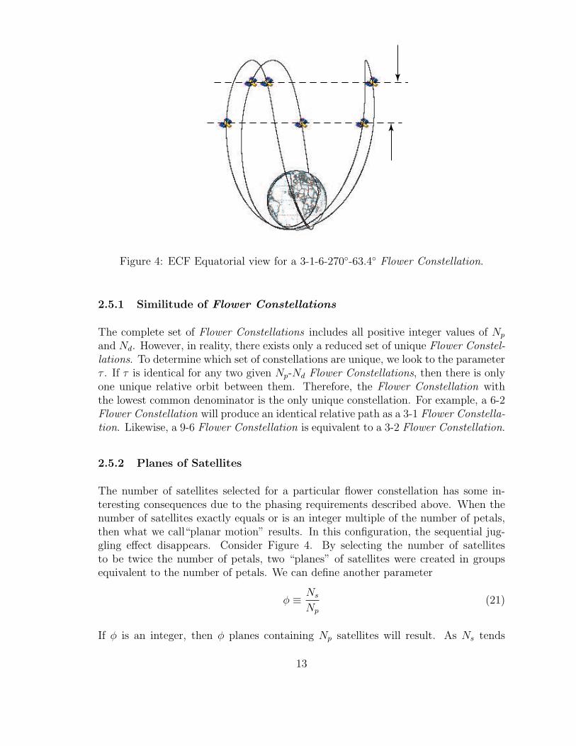
Figure 4: ECF Equatorial view for a 3-1-6-270-63.4 Flower Constellation.

2.5.1 Similitude of Flower Constellations

The complete set of Flower Constellations includes all positive integer values of Np

and Nd. However, in reality, there exists only a reduced set of unique Flower Constel-lations. To determine which set of constellations are unique, we look to the parameterτ . If τ is identical for any two given Np-Nd Flower Constellations, then there is onlyone unique relative orbit between them. Therefore, the Flower Constellation withthe lowest common denominator is the only unique constellation. For example, a 6-2Flower Constellation will produce an identical relative path as a 3-1 Flower Constella-tion. Likewise, a 9-6 Flower Constellation is equivalent to a 3-2 Flower Constellation.

2.5.2 Planes of Satellites

The number of satellites selected for a particular flower constellation has some in-teresting consequences due to the phasing requirements described above. When thenumber of satellites exactly equals or is an integer multiple of the number of petals,then what we call“planar motion” results. In this configuration, the sequential jug-gling effect disappears. Consider Figure 4. By selecting the number of satellitesto be twice the number of petals, two “planes” of satellites were created in groupsequivalent to the number of petals. We can define another parameter

φ ≡ Ns

Np

(21)

If φ is an integer, then φ planes containing Np satellites will result. As Ns tends

13

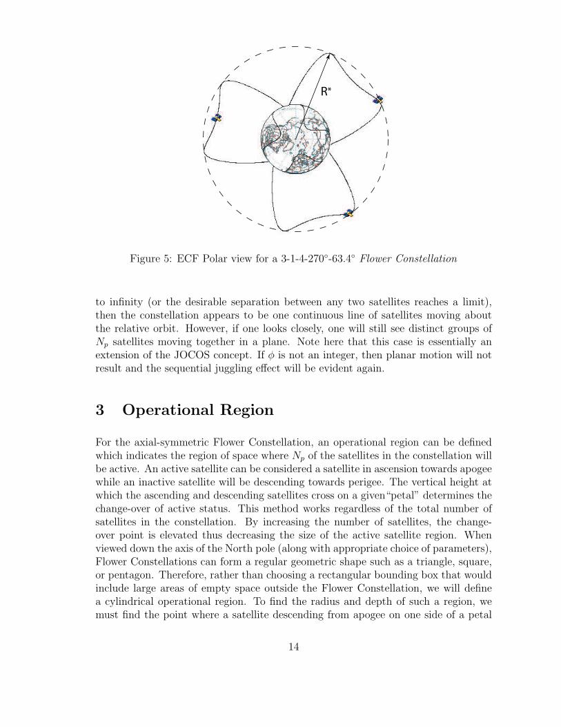
R*

Figure 5: ECF Polar view for a 3-1-4-270-63.4 Flower Constellation

to infinity (or the desirable separation between any two satellites reaches a limit),then the constellation appears to be one continuous line of satellites moving aboutthe relative orbit. However, if one looks closely, one will still see distinct groups ofNp satellites moving together in a plane. Note here that this case is essentially anextension of the JOCOS concept. If φ is not an integer, then planar motion will notresult and the sequential juggling effect will be evident again.

3 Operational Region

For the axial-symmetric Flower Constellation, an operational region can be definedwhich indicates the region of space where Np of the satellites in the constellation willbe active. An active satellite can be considered a satellite in ascension towards apogeewhile an inactive satellite will be descending towards perigee. The vertical height atwhich the ascending and descending satellites cross on a given“petal” determines thechange-over of active status. This method works regardless of the total number ofsatellites in the constellation. By increasing the number of satellites, the change-over point is elevated thus decreasing the size of the active satellite region. Whenviewed down the axis of the North pole (along with appropriate choice of parameters),Flower Constellations can form a regular geometric shape such as a triangle, square,or pentagon. Therefore, rather than choosing a rectangular bounding box that wouldinclude large areas of empty space outside the Flower Constellation, we will definea cylindrical operational region. To find the radius and depth of such a region, wemust find the point where a satellite descending from apogee on one side of a petal

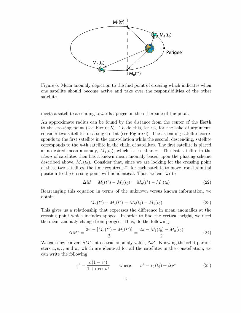
14

M1(t0)

Mn(t0)

M1(t*)

Mn(t*)

Perigee

Figure 6: Mean anomaly depiction to the find point of crossing which indicates whenone satellite should become active and take over the responsibilities of the othersatellite.

meets a satellite ascending towards apogee on the other side of the petal.

An approximate radius can be found by the distance from the center of the Earthto the crossing point (see Figure 5). To do this, let us, for the sake of argument,consider two satellites in a single orbit (see Figure 6). The ascending satellite corre-sponds to the first satellite in the constellation while the second, descending, satellitecorresponds to the n-th satellite in the chain of satellites. The first satellite is placedat a desired mean anomaly, M1(t0), which is less than π. The last satellite in thechain of satellites then has a known mean anomaly based upon the phasing schemedescribed above, Mn(t0). Consider that, since we are looking for the crossing pointof these two satellites, the time required, t∗, for each satellite to move from its initialposition to the crossing point will be identical. Thus, we can write

∆M = M1(t∗)−M1(t0) = Mn(t∗)−Mn(t0) (22)

Rearranging this equation in terms of the unknown versus known information, weobtain

Mn(t∗)−M1(t∗) = Mn(t0)−M1(t0) (23)

This gives us a relationship that expresses the difference in mean anomalies at thecrossing point which includes apogee. In order to find the vertical height, we needthe mean anomaly change from perigee. Thus, do the following

∆M∗ =2π − [Mn(t∗)−M1(t

∗)]2

=2π −M1(t0)−Mn(t0)

2(24)

We can now convert δM∗ into a true anomaly value, ∆ν∗. Knowing the orbit param-eters a, e, i, and ω, which are identical for all the satellites in the constellation, wecan write the following

r∗ =a(1− e2)

1 + e cos ν∗where ν∗ = ν1(t0) + ∆ν∗ (25)

15

z*

za∆z

Figure 7: ECF Equatorial view for a 3-1 Flower Constellation

This is the radius vector to the satellite, which we must now express in the ECI frameto find R∗.

R = RT3 (Ω)RT

1 (i)RT3 (ω + ν∗)

r∗

00

(26)

Taking the magnitude of the components in the X-Y plane, we can now find R∗. Inthe Z-axis direction, the distance from the crossing point to the apogee of the petalis considered the active region for the satellites in the constellation. We can find thisdistance by expanding the rotation matrix in Equation 26 and multiplying through,we can write

z∗ = r∗(sin ω sin i cos ν∗ + cos ω sin i sin ν∗) (27)

This implies that our operational region is found by (see Figure 7)

∆z = za − z∗ (28)

where za isza = ra sin ω sin i = a(1 + e) sin ω sin i (29)

4 Specific Cases and Potential Applications

4.1 Flower Constellations and Global Navigation Systems

One potential application of Flower Constellations is in the arena of Global Navi-gation Systems. The current GPS system consists of a large number of satellites in

16

Figure 8: ECF Equatorial view for a double 3-1-5-270-63.4 Flower Constellation.The dark shaded portions of the relative orbit indicate access is available while theblack squares indicate satellites currently available.

a Walker constellation (circular orbits). This creates a sphere of GPS satellites sur-rounding the Earth, which is ideal for broadcasting GPS signals back to the Earth’ssurface and LEO. However, this system is ill suited to sending GPS signals to MEO,HEO and GEO orbits. Figure 8 shows a double 3-1-5-270-63.4 Flower Constellationand a test case geo-stationary satellite. Using STK software, the access between thegeo-stationary satellites and the double Flower Constellation were computed. Eachof the satellites were given a sensor with a 55 cone angle. While this sensor angle isarbitrary at the moment, future work will incorporate realistic sensor models. Withthis configuration, a minimum of 4 and up to 6 accesses were available to the geo-stationary satellite. Thus, obtaining a position fix is assured because of the quasi-stationarity property of the Flower Constellations. Note here that the operationalregion definition will factor heavily into whether or not access to active satellites isavailable. More work is needed to determine sensor requirements and optimal num-ber of petals and satellites. However, we can be certain that the number of satellitesrequired to populate a Flower Constellation based GPS augmentation system will besignificantly less than that of the standard Walker constellation concept.

17

(a) (b)

(c) (d)

Figure 9: 3 ECF cardinal views (a,c,d) and an isometric view (b) of a 4-1-5-270-116.6

Flower Constellation

4.2 Formation Flying Schemes

4.2.1 Follow the Leader

Another interesting scenario arises when one selects a retrograde Flower Constella-tion. In Figure 9, a 4-1-5-270-116.6 Flower Constellation is depicted. The samephasing rules regarding a sequential juggling constellation were followed as describedabove. However, in this case, we have a “follow the leader” situation. The satel-lites rotate clockwise about the Earth in view (a). The “tail” satellite will descendtowards perigee only to reappear on the opposite side of the Earth in the “lead”position. Likewise, the next to last satellite will then descend and reappear in thelead. And additional curiosity is that, when viewed from the North Pole (view (a)),the satellites move along a perimeter which is almost square. Flower Constellationswhich form regular polygon shapes can be useful in Earth observation missions wheregridding of information is a concern.

18

ECI Orbits

ECF Relative Orbit

Figure 10: An asymmetric Flower Constellation based upon a 3-1 Flower Constella-tion. Five satellites were placed with nodes evenly arrayed in a 45 range. The meananomalies were then computed using the standard phasing rules.

4.2.2 Asymmetric Flower Constellations

Another intriguing possibility is the use of asymmetric Flower Constellations for for-mation flying. By placing a number of satellites within a given range of RAAN values,we can bunch the satellites together in such a way as to act as a formation. Figure10 shows an example of this. In this figure, both the relative orbit and the 5 inertialorbits of each satellite are shown. Additionally, one could consider having multipleFlower Constellations with multiple chains of satellites all placed within close prox-imity of each other. Future work will include efforts to apply some of the more uniqueaspects of Flower Constellations to the formation flying problem.

4.2.3 Rigid Rotation of the Axis of Symmetry

In all the preceding examples, the axis of symmetry corresponds to the Earth spinaxis. Obviously, this is intimately related to the desire to obtain repeating groundtracks. However, if there is a particular version of the Flower Constellation that hasa useful interplay between the satellites, then one can rigidly rotate the ECI orbitsof each satellite to move the axis of symmetry to some other desired direction. Theconsequences of doing this are the destruction of the repeating ground track prop-erty and the fact that control would be required to maintain the initial constellation

19

geometry. Future work is needed to study in detail the amount of control effort thatwould be required for a given configuration.

4.3 Visualization Analysis Tool

Flower Constellations have many potential applications. To aid in the analysis ofthis potential, it is important to be able to properly visualize the constellation. Formany Flower Constellations, viewing these orbits on a Mercator projection does notadequately represent the complete shape. Major software applications such as AGI’sSatellite Tool Kit are available which allow one to view three dimensional graphicsof satellite orbits. However, STK can only show ECF relative orbits in a static way(i.e. the camera can not be easily moved to view the relative orbits from any angle).Also, STK does not allow one to view the relative and inertial orbits simultaneously.Therefore, we undertook the task of creating a JAVA application which would simplifythe task of design and study of Flower Constellations. We now have a 3D animationand analysis tool that allows the user to input the six basic parameters of a FlowerConstellation along with specifying the phasing requirements (e.g. a symmetric versusasymmetric constellation). Because JAVA is relatively platform independent, oncethis tool is complete, we will be able to make this software available to other users- possibly even as a web-based application. We feel that it is virtually impossible tofully understand the implications of complex constellations without a visualizationtool of this nature.

4.4 Conclusion

In this paper, we have presented the Flower Constellation concept. We have extendedthe concepts of the Broglio Clover, LOOPUS, and JOCOS systems among others. Amethod for generating any variety of Flower Constellation was presented with meth-ods for handling known perturbations to achieve precisely repeating ground tracks.We also discussed a number of specific cases and potential applications which will bethe subject of future papers.

Further work will be performed in the application of Flower Constellations to telecom-munications, coverage, global navigation, and formation flying. While telecommuni-cations and coverage have been explored over the last decade or so to a certain extent,we feel that there are other unique applications of Flower Constellations which havenot yet been fully exploited. Additionally, we will look into the lifetime of FlowerConstellations and compare the cost to launch these kinds of constellations versusmore traditional ones.

20

4.5 Acknowledgements

The authors would like to thank the Spacecraft Technology Center (STC), formerlyknown as the Commercial Space Center for Engineering (CSCE), for the generoususe of their facilities and personnel. Specifically, Ms. Maria Puente has been ofexceptional service. We also appreciate all those who have expressed interest in theFlower Constellation concept.

References

[1] Broglio, L., “Una Politica Spaziale per il Nostro Paese, Prospettive del ProgettoSan Marco: Il Sistema Quadrifoglio,” Centro di Ricerca Progetto San Marco,Internal Report, 1981.

[2] Castronuovo, M. M., Bardone, A., and Ruscio, M. D., “Continuous Global EarthCoverage By Means of Multistationary Orbits,” Advances in the AstronauticalSciences , Vol. 99, 1998, pp. 1021–1039.

[3] Turner, A. E., “Non-Geosynchronous Orbits for Communications to Off-LoadDaily Peaks in Geostationary Traffic,” AAS Paper 87-547, 1987.

[4] Nugroho, J., Draim, J., and Hudyarto, “A Satellite System Concept for PersonalCommunications for Indonesia,” Paper Presented at the United Nations Indone-sia Regional Conference on Space Science and Technology, Bandung, Indonesia,1993.

[5] Proulx, R., Smith, J., Draim, J., and Cefola, P., “Ellipso Gear Array - Coordi-nated Elliptical/Circular Constellations,” AAS Paper 98-4383, 1998.

[6] Draim, J., “Elliptical Orbit MEO Constellations: A Cost-Effective Approach forMulti-Satellite Systems,” Space Technology , Vol. 16, No. 1, 1996.

[7] Solari, G. and Viola, R., “M-HEO: the optimal satellite system for themost highly populated regions of the northern hemisphere,” IntegratedSpace/Terrestrial Mobile Networks Action Final Summary, ESA COST 227TD(92)37, 1992.

[8] Pennoni, G. and Bella, L., “JOCOS: A Triply Geosynchonous Orbit for GlobalCommunications An Application Example,” Tenth International Conference onDigital Satellite Communications , Vol. 2, 1995, pp. 646–652.

[9] Dondl, P., “LOOPUS Opens a Dimension in Satellite Communications,” Inter-national Journal of Satellite Communications , Vol. 2, 1984, pp. 241–250, Firstpublished 1982 in German.

21

[10] Rouffet, D., “The SYCOMORES system [mobile satellite communications],” IEEColloquium on ‘Highly Elliptical Orbit Satellite Systems’ (Digest No.86), pp.6/1-6/20, 1989.

[11] Norbury, J., “The Mobile Payload of the UK T-Sat Project,” IEE Colloquiumon ‘Highly Elliptical Orbit Satellite Systems’ (Digest No.86), pp. 7/1-7/7, 1989.

[12] Draim, J. E., Inciardi, R., Cefola, P., Proulx, R., and Carter, D., “Demonstrationof the COBRA Teardrop Concept Using Two Smallsats in 8-hr Elliptic Orbits,”15th Annual/USU Conferece on Small Satellites, SSC01-II-3, 2001.

[13] Berretta, G., “The Place of Highly Elliptical Orbit Satellites in Future Systems,”IEE Colloquium on ‘Highly Elliptical Orbit Satellite Systems’ (Digest No.86), pp.1/1-1/4, 1989.

[14] Girolamo, S. D., Luongo, M., and Soddu, C., “Use of highly elliptic orbits fornew communication services,” RBCM - J. of the Braz. Soc. Mechanical Sciences ,Vol. XVI, 1994, pp. 143–149, AAS 98-172.

[15] Stuart, J. and Smith, D. J., “Review of the ESA Archimedes Study 1,” IEEColloquium on ‘Highly Elliptical Orbit Satellite Systems’ (Digest No.86), pp.2/1-2/4, 1989.

[16] Carter, D., “When is the Groundtrack drift rate zero?” CSDL MemorandumESD-91-020, 1991, Cambridge, MA: Charles Stark Draper Laboratory.

[17] Vallado, D. A., Fundamentals of Astrodynamics and Applications , McGraw-Hill,New York, 2nd ed., 2001.

22