UPPSALA UNIVERSITET Nationalekonomiska institutionen Examensarbete magisteruppsats Master's Thesis Vårterminen 2007

The Forecasting Power of Economic Growth Models

Author: Andreas Bryhn Supervisor: Johan Lyhagen

Abstract

High forecasting power is essential for understanding scientific relationships. In economics,

forecasting power may be decisive for the success or failure of a particular policy. The

forecasting power of economic growth models is investigated in this study. Regressions from

one dataset including the gross domestic product (GDP), GDP growth, trade openness, the

quality of public institutions and secondary education generate insufficient forecasting power

with respect to growth. Furthermore, the International Monetary Fund's one-year growth

forecasts are compared to outcome. Forecasts for 1999-2006 were found to be significantly

different from outcome during 7 years out of 8. The forecast error slightly exceeded 1

percentage unit, which is similar to results from earlier studies on forecast error and equal to

the forecast/hindcast error from a simple multivariate model constructed from historical

growth data. Possible reasons behind poor forecast quality are discussed, including the

tradition to build models using assumptions from irrefutable theoretical constructs.

Sammanfattning

Hög prognoskraft är nödvändigt för förståelsen av vetenskapliga samband. Inom

nationalekonomin kan prognoskraften vara avgörande för huruvida en viss ekonomisk politik

kommer att lyckas eller misslyckas. Ekonomiska tillväxtmodellers prognoskraft undersöks i

denna studie. Regressioner från ett dataset som innehåller bruttonationalprodukten, tillväxten

hos densamma, öppenhet för handel, offentliga institutioners kvalitet, samt andel

gymnasieutbildade, genererar otillräcklig prognoskraft med avseende på tillväxt. Vidare

jämförs Internationella Valutafondens ettårsprognoser med utfall. Prognoser för 1999-2006

var signifikant skilda från utfall under 7 år av 8. Prognosfelet uppgick till drygt 1

procentenhet, vilket motsvarar resultat från tidigare studier av prognosfel, liksom prognosfelet

från en enkel, flervariabelsmodell som är baserad på historiska tillväxtdata. Möjliga

anledningar till den låga prognoskvaliteten diskuteras, däribland traditionen att bygga

modeller med hjälp av antaganden från teoretiska konstruktioner som inte kan falsifieras.

1

TABLE OF CONTENTS

Page

1. INTRODUCTION

2. METHODS AND DATA

2.1. Statistical methods and considerations

2.2. The Gallup dataset

2.3. The IMF dataset

3. RESULTS

3.1. Cross-country growth regressions

3.2. The IMF's growth forecasts

4. DISCUSSION

5. CONCLUSIONS

REFERENCES

3

5

5

6

6

7

7

9

13

17

18

2

1. INTRODUCTION

Forecasting the future has been a highly desirable goal for humans ever since the Stone Age.

With the emergence and growth of science, our forecasting methods have improved

considerably, as forecasting power has become a fundamental part and a distinguishing

feature of scientific knowledge. The ability to make accurate forecasts of important goal

variables is essential for the understanding of scientific relationships, particularly with respect

to causality (Blaug, 1980; DeLurgio, 1998; Fildes and Stekler, 2002). High forecasting power

is necessary but not sufficient for causal analysis in economics, because strongly correlated

variables may have an external, cointegrating causal factor (Clements and Hendry, 1999).

Nevertheless, without high forecasting power, economists will have poor quantitative

knowledge about the effect of their suggested policies on, e. g., economic growth. Insufficient

forecasting power may therefore result in disappointing and expensive policy failure.

The forecasting power of a model can be estimated by calculating the correlation coefficient

(R2) for the relationship between model forecasts and actual outcome. Two crucial issues in

this context are (1) the relative quality of models; i. e., how much better is, e. g., R2 = 0.9,

compared to R2 = 0.8 in a regression between forecast and outcome, and (2) the lower limit of

acceptability, as measured in R2. If there is a large enough amount of data, a correlation with

R2 very close to 0 can still be significant at high confidence levels, but it will be just as

useless for forecasting as a correlation with R2 = 0, because in both cases, correlations will

describe a beeswarm-like scatterplot from which forecasts will have very high uncertainty.

One widely used lower limit of acceptability regarding R2 and forecasting power was first

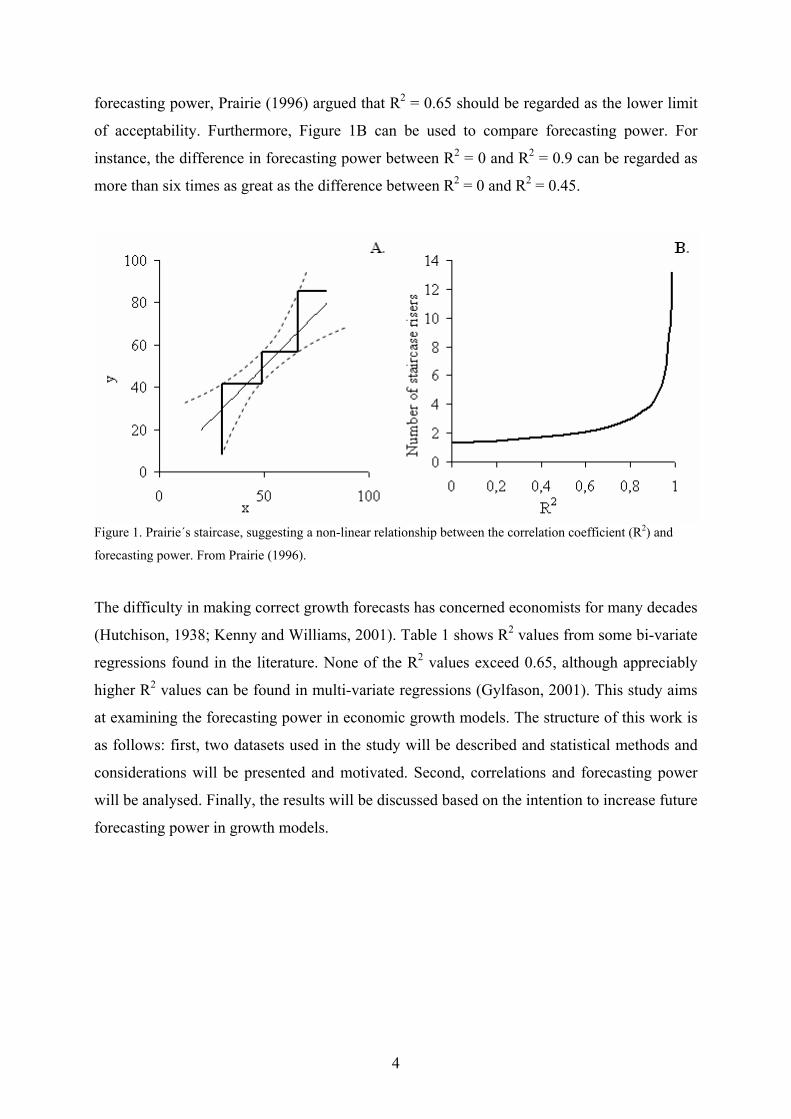
motivated by Prairie (1996), who presented what has become known in the natural sciences as

Prairie's staircase. Prairie's staircase method is illustrated in Figure 1A. A thick, solid line

starts at the lower boundary line of the 95 % confidence level from the regression and is

drawn upwards until it reaches the upper 95 % confidence limit, and is then drawn to the right

until the lower boundary line is reached again. This procedure is repeated so that the thick,

solid line takes the shape of a staircase (Figure 1A). When Prairie (1996) reiterated this

exercise for a large number of correlations, he found a non-linear relationship between R2 and

the number of staircase risers, which is depicted in Figure 1B. According to this figure, the

number of risers is low and fairly constant for R2 values from 0 to about 0.65, after which the

number rises rather dramatically. Using the number of staircase risers as a representation of

3

forecasting power, Prairie (1996) argued that R2 = 0.65 should be regarded as the lower limit

of acceptability. Furthermore, Figure 1B can be used to compare forecasting power. For

instance, the difference in forecasting power between R2 = 0 and R2 = 0.9 can be regarded as

more than six times as great as the difference between R2 = 0 and R2 = 0.45.

Figure 1. Prairie´s staircase, suggesting a non-linear relationship between the correlation coefficient (R2) and

forecasting power. From Prairie (1996).

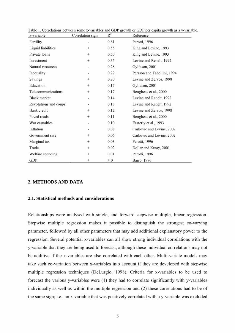
The difficulty in making correct growth forecasts has concerned economists for many decades

(Hutchison, 1938; Kenny and Williams, 2001). Table 1 shows R2 values from some bi-variate

regressions found in the literature. None of the R2 values exceed 0.65, although appreciably

higher R2 values can be found in multi-variate regressions (Gylfason, 2001). This study aims

at examining the forecasting power in economic growth models. The structure of this work is

as follows: first, two datasets used in the study will be described and statistical methods and

considerations will be presented and motivated. Second, correlations and forecasting power

will be analysed. Finally, the results will be discussed based on the intention to increase future

forecasting power in growth models.

4

Table 1. Correlations between some x-variables and GDP growth or GDP per capita growth as a y-variable. x-variable Correlation sign R2 Reference Fertility - 0.61 Perotti, 1996 Liquid liabilities + 0.55 King and Levine, 1993 Private loans + 0.50 King and Levine, 1993 Investment + 0.35 Levine and Renelt, 1992 Natural resources - 0.28 Gylfason, 2001 Inequality - 0.22 Persson and Tabellini, 1994 Savings + 0.20 Levine and Zervos, 1998 Education + 0.17 Gylfason, 2001 Telecommunications + 0.17 Bougheas et al., 2000 Black market - 0.14 Levine and Renelt, 1992 Revolutions and coups - 0.13 Levine and Renelt, 1992 Bank credit + 0.12 Levine and Zervos, 1998 Paved roads + 0.11 Bougheas et al., 2000 War casualties - 0.10 Easterly et al., 1993 Inflation - 0.08 Carkovic and Levine, 2002 Government size + 0.06 Carkovic and Levine, 2002 Marginal tax + 0.03 Perotti, 1996 Trade + 0.02 Dollar and Kraay, 2001 Welfare spending + 0.01 Perotti, 1996 GDP + ≈ 0 Barro, 1996

2. METHODS AND DATA

2.1. Statistical methods and considerations

Relationships were analysed with single, and forward stepwise multiple, linear regression.

Stepwise multiple regression makes it possible to distinguish the strongest co-varying

parameter, followed by all other parameters that may add additional explanatory power to the

regression. Several potential x-variables can all show strong individual correlations with the

y-variable that they are being used to forecast, although these individual correlations may not

be additive if the x-variables are also correlated with each other. Multi-variate models may

take such co-variation between x-variables into account if they are developed with stepwise

multiple regression techniques (DeLurgio, 1998). Criteria for x-variables to be used to

forecast the various y-variables were (1) they had to correlate significantly with y-variables

individually as well as within the multiple regression and (2) these correlations had to be of

the same sign; i.e., an x-variable that was positively correlated with a y-variable was excluded

5

if its contribution in the multiple regression was negative, and vice versa. These criteria are

not commonly used in econometrics (DeLurgio, 1998) and their relevance will therefore be

discussed later in this paper. Changes in linear slopes were detected with a trend shift analysis

method from Rodionov and Overland (2005). This method consists of a downloadable

application to Microsoft Excel and makes it possible to detect at which points a trend changes

at a specified significance level, given that the trend changes at all. Statistical significance

was always determined at the 95 % confidence level, since Figure 1 is defined at that level.

2.2. The Gallup dataset

The first dataset (CID, 2007) of two used in this study has been described by Gallup et al.

(1999) and was used in regression 1, Table 3 in the same study. It consists of six variables;

average purchasing power parity (PPP) adjusted annual gross domestic product (GDP) per

capita growth between 1965 and 1990 (hereafter called yG), PPP adjusted initial GDP per

capita in 1965 (hereafter referred to as YG), average years of secondary schooling among the

population in 1965 (EduG), the log value of life expectancy (LifeG), openness to international

trade (OpenG), and finally, the quality of public administration (PublG). This dataset was used

in Section 3.1, first to estimate bi-variate correlations with yG, and subsequently, to

quantitatively assess multi-variate correlations with yG using the criteria stated in 2.1. The

dataset was then divided into groups according to the gradient of one variable which was

insignificantly correlated with yG, to investigate whether the effect of such a variable on other

regressions could be estimated without violating the criteria in 2.1.

2.3. The IMF dataset

The second dataset consisted of actual and forecasted data on PPP adjusted GDP growth in 29

advanced economy in 10 of the International Monetary Fund's (IMF) April or May issues of

World Economic Outlook (IMF, 1998, 1999, 2000, 2001, 2002, 2003, 2004, 2005, 2006,

2007). In this work, yt denotes historical IMF data on growth at time t (in years), and it is

worth noting that IMF data are not given as per capita values, as opposed to yG. One-year

growth forecasts (yfort+1) were first compared to the actual outcome (yt+1) in a bi-variate

regression, and the resulting R2 value was compared to R2 values found between historical

data at the time of the forecast and yt+1.

6

A statistical model based on the presented historical data at the time of the forecast was then

used as a baseline from which to evaluate the forecast quality. This statistical model was

developed from a stepwise multiple regression with yt+1 as a y-variable and all historical data

available at the time of the forecast as potential x-variables. The baseline model was based on

the time period 1998 ≤ t ≤ 2004, i. e., on growth outcome from 7 years and 29 OECD

countries. In order to test the criteria in 2.1 by violating them, 100 normal distributed random

variables were added to the data set, allowing all significant x-variables to enter into the

forward stepwise multiple regression with yt+1 as a y-variable. If any of the random variables

would enter, then that would indicate that the criteria in 2.1 could decrease the risk of adding

nonsensical information to the regression.

The stability of the model constants were subsequently studied by omitting data from one year

at the time. Forecasts/hindcasts from the statistical model were tested against yt+1 by using

those model constants which were valid for all years except for the particular

forecast/hindcast year, in order to perform a test against "independent" data in the sense that

they were not used to develop the statistical model. For example, when hindcasting yt+1 for t =

2001, the model constants used were those that were valid for a multiple regression when t =

2001 had been omitted. Furthermore, the baseline model with constants valid for 1998 ≤ t ≤

2004 was tested to forecast yt+1 for t = 2005, a year from which data had previously not been

used at all in the study. These forecasts were compared to the IMF's forecasts (IMF, 2005)

and to the actual outcome (IMF, 2007). Finally, error terms from all forecasts and hindcasts in

this section were studied and compared.

3. RESULTS

3.1. Cross-country growth regressions

Table 2 displays cross-correlations (R2 values) between the six variables in Gallup et al.

(1999), described in Section 2. All correlations carried a positive sign. According to Table 2,

EduG, LifeG, OpenG and PublG were all mutually correlated and also positively correlated with

yG. YG was insignificantly - although, if anything, positively - correlated with yG.

7

Table 2. Cross-correlations (n=75) between six variables described in Section 2 and by Gallup et al., (1999). * =

significant at the 95 % confidence level.

YG yG EduG LifeG OpenG yG 0.00 EduG 0.39* 0.14* LifeG 0.51* 0.22* 0.60* OpenG 0.32* 0.38* 0.33* 0.40* PublG 0.61* 0.19* 0.39* 0.48* 0.53*

Thus, all variables except YG could be used in a multi-variate model according to the criteria

set in Section 2. The baseline equation for this model is:

yG = a + b · EduG + c · LifeG + d · OpenG + e · PublG (1)

where a-e are constants. However, only OpenG could enter as a significant x-variable in a

forward stepwise multiple regression with yG as a y-variable. Therefore, constants b, c, and e

were not determined, while a (including its standard error) was 0.787 ± 0.244 (p = 0.002, t =

3.23) and d was 2.62 ± 0.38 (p < 0.001, t = 6.74).

Table 3 shows how the R2 value changed when the data were divided into groups along the

YG gradient. When the data were grouped into 2, the R2 for OpenG vs. yG increased from 0.39

to 0.45 for the poorest countries (cases 1-48), and from 0.39 to 0.40 for the richest countries

(cases 49-96). Growth in the group with the poorest countries could also be forecasted with a

multiple regression that rendered an R2 value of 0.53 and included openness and log values of

life expectancy in 1965 as x-variables.

Table 3. Regression analysis with yG as a y-variable. The data set was sorted ascendingly according to the level

of YG.

Cases

n

Highest R2, single regression

Variable in single regression

R2, multiple regression

Variable(s) in multiple regression

1-96 94 0.39 OpenG 0.39 OpenG 1-48 48 0.45 OpenG 0.53 OpenG, LifeG 49-96 46 0.40 OpenG 0.40 OpenG 1-32 32 0.39 OpenG 0.39 OpenG 33-64 31 0.42 OpenG 0.58 OpenG, LifeG 65-96 31 0.50 OpenG 0.50 OpenG

When data were grouped into 3, R2 increased further for the richest third (cases 65-96) to 0.50

and the middle group (cases 33-64) allowed log life expectancy to enter as an additional x-

8

variable in the multiple regression, yielding an R2 value of 0.58. However, when the data was

divided into more groups than 3, regressions became insignificant in many of the groups. A

trend shift analysis of the OpenG vs. yG relationship using the method from Rodionov and

Overland (2005) showed that there were no significant slope deviations in the openness-

growth relationship along the GDP per capita gradient. Likewise, a t-test revealed that the

regression slope was slightly but insignificantly steeper among the poorest half of the

countries compared to the richest half.

3.2. The IMF's growth forecasts

The first row in Table 4 gives the

correlation between the IMF's GDP growth

forecasts and the actual outcome one year

after the forecast. The subsequent rows

contain correlations between historical

GDP growth data at the time of the

forecast, and the GDP growth one year

after. All significant correlations were

positive. It is worth noting that two

historical variables in Table 4 yielded

equal or higher R2 values against outcome

as compared to IMF's forecasts.

Table 4. Correlations (n=190) between the IMF's

growth forecasts or historical growth data, and

growth one year after the forecast. Data from IMF

(1998, 1999, 2000, 2001, 2002, 2003, 2004, 2005,

2006). All correlations were significant at the 95 %

confidence level. MV denotes the mean value.

Variable R2 Yfor

t+1 0.15 yt-1 0.04 yt-2 0.08 yt-3 0.10 yt-4 0.18 yt-5 0.06 yt-6 0.03 yt-7 0.04 yt-8 0.09 MV(yt-18, yt-17, …, yt-9) 0.15

A multiple regression with yt-1, yt-2, …, yt-8, and the mean value of yt-18, yt-17, …, yt-9 as x-

variables and the future growth outcome yt+1 as an y-variable allowed three historical data

variables to enter at the 5 % significance level, raising the R2 value to 0.26. From this

regression, the following statistical model was constructed:

),...,,( 91718421 −−−−−+ ⋅+⋅+⋅+= tttttt yyyMViyhygfy (2)

where f-i were constants which were determined to f = 0.670, g = 0.162, h = 0.273 and i =

0.246.

9

When 100 normal distributed random variables were added to the data set, violating the

criteria stated in 2.1, the resulting regression generated an R2 value of 0.35, and included yt-2,

yt-4, yt-7, yt-8, and 5 of the random variables as significant x-variables. None of the random

variables was significantly correlated with yt+1 in a single regression. When the random

variables were removed from the regression, yt-7 remained as a significant x-variable, but with

a negative sign. In an attempt to use yt-7 as an explanatory variable in compliance with the

criteria in 2.1, 8 new variables were generated with yt-7 as a denominator and the 8 other

historical variables from the IMF dataset as nominators. However, none of these ratios were

correlated with yt+1. Likewise, no significant correlation with yt+1 could be generated from

variables that consisted of yt-7 subtracted from any of the remaining historical variables in the

IMF dataset.

The stability of the constants in Equation 2 was tested by omitting yt+1 from one year at the

time and the results are displayed in Table 5. g could not be significantly separated from 0 for

one of the years (t+1 = 2001). The coefficient of variation (CV) for h was only 3.3%,

indicating a comparatively stable contribution to Equation 2 from yt-4 in relation to the other

historical variables.

Table 5. The stability of the constants in Equation 2 when yt+1 from one year at a time was omitted. The first

column describes which one of the forecasted years was excluded from the analysis. MV denotes mean value,

SD is the standard deviation and CV is the coefficient of variation and equals SD/MV. *Based on t+1 = 1999,

2000, 2002-2005. **Not significantly different from zero.

Excluded t+1 f g h i R2 None 0.670 0.162 0.273 0.246 0.26 1999 0.708 0.265 0.270 0.266 0.22 2000 0.806 0.107 0.257 0.234 0.23 2001 0.628 ** 0.283 0.405 0.31 2002 0.632 0.157 0.271 0.258 0.24 2003 0.558 0.217 0.276 0.230 0.28 2004 0.616 0.269 0.281 0.143 0.28 2005 0.630 0.163 0.261 0.263 0.23 MV* 0.658 0.196 0.269 0.232 0.25 SD* 0.087 0.065 0.009 0.046 0.03 CV* 0.132 0.331 0.033 0.199 0.11

The IMF's forecasts were compared to growth forecasts/hindcasts generated by Equation 2 by

regressing forecasts and hindcasts against GDP growth outcome, and these regressions are

10

shown in Figure 2. As motivated in the previous section, constants f-i were taken from Table

5 in order to test hindcasts from Equation 2 against independent data; i.e., the growth outcome

(yt+1) of, e. g., 2003 was compared to hindcasts from Equation 2 with constant values for f-i

taken from the 2003 line in Table 5. It is worth noting that for 1999 ≤ t+1 ≤ 2004, Equation 2

yielded hindcasts since constants were also generated from yt+1 data from subsequent years,

while the same equation yielded forecasts for 2005 since the information on the 2005 line in

Table 5 strictly emanates from years that preceded 2005. The regression slopes in Figure 2 are

both less than 1, indicating that forecasts and hindcasts may be systematically higher than the

outcome. However, mean values of forecasts, hindcasts and outcome all slightly exceeded 3%

and were not significantly different from one another. Thus, forecasts/hindcasts < 3% showed

a tendency to be overestimated compared to the real outcome yt+1, while forecasts/hindcasts >

3% tended to be underestimated, which explains why the regressions in Figure 2 differed from

the unit line (y=x).

Figure 2. Comparison between one-year forecast/hindcasts and outcome in yearly GDP growth (%) 1999-2005.

A. Forecasts from the IMF's World Economic Outlook. B. Forecasts/hindcasts from Equation 2.

The R2 value in Figure 2B was low, at 0.19, although marginally higher than in Figure 2A

(0.15). According to Figure 2A, none of the IMF's growth forecasts were negative, and none

exceeded 7.2 percent, although negative growth was observed in 9 cases out of 195 and higher

growth than 7.2 percent was observed in 12 cases.

Forecasts from IMF (1995) and Equation 2 compared to outcome (IMF, 2007) regarding GDP

growth in 2006 are displayed in Figure 3. The IMF's forecasts (Figure 3A) yielded a rather

high R2 value (0.55) when regressed against growth outcome, much higher than forecasts

11

from Equation 2 (0.19, see Figure 3B). However, the two regression equations in Figure 3

show that R2 values rather inaccurately reflected the forecasting power in this case, because

forecasts from both sources were systematically and significantly lower than outcome.

Figure 3. Comparison between one-year forecasts and outcome in GDP growth (%) 2006. A. Forecasts from the

IMF's World Economic Outlook. B. Forecasts from Equation 2.

The differences between the IMF's forecasts, forecasts/hindcasts from Equation 2, and

outcome, are further illustrated in Figure 4. Apparently, errors from both methods followed a

very similar pattern with respect to mean error and standard deviation of the error. During an

average year, the absolute value of the mean error was 1.1 percentage units while the standard

deviation of the error slightly exceeded 1.5 percentage units. Figures 4B and 4C suggest that

forecasts improved over time, given the slightly decreasing mean error deviation from 0 and

the slightly decreasing standard deviation of the error. However, the difference between IMF's

forecasts and growth outcome (including the bars representing the mean value error) in Figure

4A shows that IMF's forecasts were significantly different than outcome for all years except

for 2005. Forecasts/hindcasts from Equation 2 significantly deviated from outcome for all

years except for 1999 and 2005. Thus, 2005 appeared to be an outstandingly predictable year

(mean relative error < 10% according to Figure 4D) while the year 2001 was very

unpredictable (mean relative error > 70%) with respect to GDP growth.

12

Figure 4. Accuracy in GDP growth forecasting. A. Mean GDP growth forecasts for 29 OECD countries from the

IMF's World Economic Outlook, compared to mean values generated by Equation 2 (hindcasts for 1999-2004

and forecasts for 2005-2006), and to outcome, including the mean value error. Values in percent. B. The mean

forecast/hindcast error in percentage units of GDP growth. B. The standard deviation (SD) of the growth

forecast/hindcast error. C. The relative error (forecast or hindcast error divided by outcome) in percent.

4. DISCUSSION

Many economic growth models are motivated by economic theory and contain common

theoretical assumptions about, e. g., perfect competition (Ventura, 2005). There is reason to

question whether this method is optimal for constructing growth models. Karl Popper's strict,

generic, and unambiguous demarcation line between science and non-science (metaphysics or

pseudo-science) has since its first publication in 1934 widely gained respect in the scientific

13

community as a fundamental part of the hypothetico-deductive method. A primary criterion

for a scientific theory according to this demarcation method is that the theory must be

refutable, i.e., it must be possible to falsify the theory with evidence of the opposite. A

subsequent criterion is that the theory must pass some kind of empirical test. These criteria

have laid the ground for substantial progress in many academic disciplines. Irrefutable

constructs may very well have a heuristic value or play other important roles in inspiring the

future development of scientific theories. However, only refutable scientific theory has the

potential to forecast and to explain relationships by including probable outcomes and

excluding improbable outcomes. Separating scientific theory from metaphysics and

specifying their separate roles have the potential to improve the forecasting power and thus

the understanding of scientific relationships. Every time a scientific theory is refuted and

improved, the new theory brings us one step closer to the unattainable goal; the "truth"

(Popper, 1972).

The need to use refutability as a scientific criterion in economics has been acknowledged by

many economists (e. g., Hutchison, 1938; Blaug, 1980; Eichner, 1985; Stanley, 1998;

Bernhofen, 2005). Those who oppose this criterion (see, e. g., Hands, 2001 and references

therein) have thus far failed to present an alternative demarcation line which unambiguously

classifies astrology, alchemy and religion as non-science. Many economic theories which

have been found irrefutable assume conditions that cannot be observed, such as steady-state,

perfect competition and ceteris paribus, or contain empirically empty assumptions such as

rational behaviour; although every kind of behaviour may be considered rational by those who

display it (Hutchison, 1938; Blaug, 1980).

An example of an irrefutable theory is the well-known principle of comparative advantage.

This principle can be demonstrated by a logical exercise which shows that trade is always

beneficial for everyone involved. Evidently, no real observations of trade being harmful (e. g.,

arms trade between countries at war with each other, or narcotics trade with a subsequent

increase in drug addiction and social costs) has the potential to falsify, or even affect, this

logical exercise. In other words, the principle has no empirical content and cannot convey any

information about economic relationships in the real world. Bernhofen (2005) objected that

the principle of comparative advantage is indeed refutable, since the opposite of the principle

(trade being harmful) is a possible outcome. However, refutability requires that a theory does

not only have an opposing hypothesis, but that the theory may also be falsified with evidence

14

of the opposite (Popper, 1972). Opposing evidence is therefore more important than

confirmative evidence for a refutability test. Consequently, the principle of comparative

advantage can certainly be used to illustrate the correlation between openness to trade and

growth, as found in Table 2, but the principle should not be trusted as a pathfinder in the quest

for forecasting power. Likewise, neo-classical growth theory, which forecasts growth

convergence, hinges on conditions that have yet to be observed, such as perfect competition

and market equilibrium. As a result, observed growth divergence cannot possibly refute the

convergence hypothesis (Meeusen, 2003), because convergence can always be suspected to

occur sometime in the near or distant future, even if there are no present signs of it.

This line of reasoning brings us back to the reasons for not allowing YG to enter as an x-

variable with a negative sign in a multiple regression with yG as a y-variable. This choice has

been made in the present study, as opposed to, e. g., Gallup et al. (1999) and references

therein. The first reason why this choice was made here is that such a regression would

forecast that growth is lower in rich countries than in poor countries, which would contradict

Table 2, which instead forecasts that the relationship between YG and yG is insignificant, and,

if anything, positive (also supported by Barro, 1996). Furthermore, the analysis of the OpenG

vs. yG relationship showed that the regression slope was rather constant all along YG gradient,

indicating no significant effect from YG in this respect. Second, the "normal" reason for

ignoring results from individual correlations when constructing multi-variate models consists

of references to economic theory (DeLurgio, 1998). The convergence theory, which would be

needed to justify the use of YG in a negative correlation with yG, is irrefutable, as has been

demonstrated above, and therefore ill-suited for forecasting. Third, since YG is non-stationary

and yG is its derivative, any linear combination between YG and yG will have a non-stationary

residual with an infinite variance (Jones, 1995; Clements and Hendry, 1999). Instead of using

YG as a determinant of yG, a non-linear model can be constructed which varies according to

YG. Table 3 indicates that such a model can increase the forecasting power compared to a

linear model, since the R2 value increased when the dataset was divided into groups according

to YG values.

Future use of the criteria suggested in 2.1 is also motivated by the observation that when these

criteria were violated, several random variables could enter as significant determinants of

GDP growth in a multiple regression including historical growth data. This implies that if a

variable which shows no individual correlation with growth is used in a multiple regression,

15

the contribution of such a variable may very well be spurious. This may explain why many

multivariate growth regressions which generate high R2 values sometimes contain explanatory

variables with contradicting policy implications (Kenny and Williams 2001). Most of the

multivariate growth models examined by Levine and Renelt (1992) were fragile to small

changes, which should be another reason for questioning the commonly used criteria for

explanatory variables in multiple regression analysis. A final defence of the criteria set in 2.1

is that these criteria were successfully used to develop Equation 2, whose forecasts/hindcasts

were not less certain than the IMF's forecasts (Figure 4).

Similar methodological inconsistencies as those discussed above may have been fed into

many growth regressions, as well as into other types of forecasting models. Conspicuously

enough, the IMF's growth forecasts were found in this study to be of equally poor quality as

simple forecasts and hindcasts constructed from historical statistics (see Equation 2 and

Figures 2-4). These results are consistent with the findings regarding the reliability of the

World Bank's (Verbeek, 1999) and the OECD's (Pons, 1999) growth forecasts in the 1990s. In

an extensive review, Fildes and Stekler (2002) found that typical one-year growth forecasts

deviate slightly more than 1 percentage unit from outcome, which is similar to the findings in

this work (1.1 percentage units). Growth forecasts tend to be more uncertain the longer the

time-horizon (Pons, 1999) and many long-term forecasts have turned out to be grossly

inaccurate (Kenny and Williams, 2001).

Prairie's staircase (Prairie, 1996) provided a useful acceptance limit for forecasting power in

the comparison between growth forecasts/hindcasts and outcome. The IMF's forecasts and

Equation 2 generated different R2 values when regressed against outcome and all values were

below 0.65 (Figures 2 and 3) although both methods yielded rather similar errors (Figure 4).

However, the variation in regression equations from Figures 2 and 3 indicates that the

regression slope must, in addition to the R2 value, be taken into consideration in the

evaluation of forecasting power. None of the other growth regressions examined in this study

exceeded the acceptance limit (see Section 1) of R2 = 0.65. Given that many of the R2 values

in Table 1 may be at least partly additive, it may very well be possible in the future to develop

robust growth models with sufficient forecasting power, although there is reason to question

the prospects of such attempts. Forecasts of growth and other macroeconomic indicators have

not improved over time, despite extensive macroeconomic research (Fildes and Stekler,

16

2002). Ormerod and Mounfield (2000) argued that the great inherent variability in growth

statistics makes forecast failure inevitable.

The forecasting power of growth models should not be seen as a marginal issue. As stressed

in Section 1, the demonstrated shortcomings in contemporary growth forecasting may have

extensive impacts on policy outcome. The global aggregate GDP per capita growth, as well as

GDP per capita growth in many countries, have been substantially lower during recent

decades, a period often referred to as the "age of globalisation" or the "neoliberal order",

compared to preceding decades - despite the fact that policy has often been designed

according to the mainstream view among economists about the causes of growth (Rodrik,

1999; Maddison, 2001; Milanovic, 2003; Weisbrot et al., 2006). If growth forecasts would

improve in the future, this would imply that the present poor predictive understanding of

economic growth has been part of the reason why the long-term growth during recent decades

has generally not surpassed, or even reached, the high levels achieved during the "Golden

Age" of the 1950s and 1960s.

5. CONCLUSIONS

This study has evaluated the forecasting power of economic growth models and found that all

investigated models yield very uncertain forecasts, and that these findings have strong support

in the literature. The IMF's growth forecasts were significantly different than outcome in 7

years out of 8, and the forecast error was similar to that of a simple statistical model based on

historical data. One reason for the observed poor forecasting power may be the frequent use

of metaphysical constructs in growth models. Another reason may be that many growth

models include explanatory variables which show no individual correlation with growth, or

which are assumed to have an opposite, "concealed" effect, in relation to what is implied from

the variables' individual correlations with growth. Such growth models may be fragile to

small changes and may even produce contradictory policy implications, in addition to yielding

unreliable forecasts which may in turn cause extensive policy failure.

17

REFERENCES

Barro, R. J., 1996. Determinants of Economic Growth: A Cross-Country Empirical Study.

NBER Working Paper 5698. NBER, Cambridge, Massachusetts, 118 p.

Bernhofen, D. M., 2005. The Empirics of Comparative Advantage: Overcoming the Tyranny

of Nonrefutability. Review of International Economics, 13: 1017-1023.

Blaug, M. 1980. The Methodology of Economics. Cambridge University

Press, Cambridge, 314 p.

Bolaky, B. and C. Freund, 2004. Trade, Regulations, and Growth. Research working paper

WPS 3255, World Bank, Washington, 40 p.

Bougheas, S., Demetriades, P. O., and Mamuneas, T. P., 2000. Infrastructure, Specialization,

and Economic Growth. The Canadian Journal of Economics, 33: 506-522.

Carkovic, M. and Levine, R., 2002. Does Foreign Direct Investment Accelerate Economic

Growth? Working paper, University of Minnesota.

CID, 2007. http://www.cid.harvard.edu/ciddata/ciddata.html

Clements, M. P., and Hendry, D. F., 1999. Forecasting Non-stationary Economic Time Series.

The MIT Press, Cambridge, Massachusetts, 362 p.

DeLurgio, S. A., 1998. Forecasting principles and applications. Irwin/McGraw-Hill, Boston,

802 p.

Dollar, D. and A. Kraay, 2004. Trade, Growth, and Poverty. The Economic Journal, 114: F22-

F49.

Easterly, W., Kremer, M., Pritchett, L., and Summers, L. H., 1993. Good Policy or Good

Luck? Country Growth Performance and Temporary Shocks. Journal of Monetary

Economics, 32: 459-483.

18

Eichner, A. S., 1985. The lack of progress in Economics. Nature, 313: 427-428.

Fildes, R., and Stekler, H., 2002. The state of macroeconomic forecasting. Journal of

Macroeconomics, 24: 435-468.

Gallup, J.L., Sachs, J.D. and Mellinger, A.D., 1999. Geography and economic development.

International Regional Science Review 22, 179–232

Gylfason, T., 2001. Natural resources, education, and economic development. European

Economic Review, 45: 847-859.

Hands, D. W., 2001. Economic methodology is dead - long live economic methodology:

thirteen theses on the new economic methodology. Journal of Economic Methodology, 8: 49-

63.

Hutchison, T. W., 1938. The Significance and Basic Postulates of Economic Theory.

Macmillan and Co., London, 192 p.

IMF, 1998. IMF World Economic Outlook (May issue). IMF, Washington, D. C., 221 p.

IMF, 1999. IMF World Economic Outlook (May issue). IMF, Washington, D. C., 223 p.

IMF, 2000. IMF World Economic Outlook (May issue). IMF, Washington, D. C., 289 p.

IMF, 2001. IMF World Economic Outlook (May issue). IMF, Washington, D. C., 234 p.

IMF, 2002. IMF World Economic Outlook (April issue). IMF, Washington, D. C., 225 p.

IMF, 2003. IMF World Economic Outlook (April issue). IMF, Washington, D. C., 252 p.

IMF, 2004. IMF World Economic Outlook (April issue). IMF, Washington, D. C., 276 p.

IMF, 2005. IMF World Economic Outlook (April issue). IMF, Washington, D. C., 277 p.

19

IMF, 2006. IMF World Economic Outlook (April issue). IMF, Washington, D. C., 253 p.

IMF, 2007. IMF World Economic Outlook (April issue). IMF, Washington, D. C., 287 p.

Jones, C. I., 1995. Time Series Tests of Endogenous Growth Models. Quarterly Journal of

Economics, 110: 495-525.

Kenny, C. and D. Williams, 2001. What Do We Know About Economic Growth? Or, Why

Don't We Know Very Much? World Development, 29:1-22.

King, R. G., and Levine, R., 1993. Finance and Growth: Schumpeter Might be Right. The

Quarterly Journal of Economics, 108: 717-737.

Levine, R., and Renelt, D., 1992. A Sensitivity Analysis of Cross-Country Growth

Regressions. The American Economic Review, 82: 942-963.

Levine, R., and Zervos, S., 1998. Stock Markets, Banks, and Economic Growth. The

American Economic Review, Vol. 88, No. 3. (Jun., 1998), pp. 537-558.

Maddison, A., 2001. The World Economy: A Millennial Perspective. OECD, Paris, 388 p.

Meeusen, W., 2003. Economic Convergence, the ‘Stylised Facts of Growth’ and

Technological Progress. An introduction from the perspective of the theory of growth. CESIT

Discussion paper No 2003/03. University of Antwerp, Antwerp, 21 p.

Milanovic, B., 2003. The Two Faces of Globalization: Against Globalization as We Know It.

World Development, 31: 667-683.

Ormerod, P., and Mounfield, C., 2000. Random matrix theory and the failure of macro-

economic forecasts. Physica A: Statistical Mechanics and its Applications, 280: 497-504.

Perotti, R., 1996. Growth, Income Distribution, and Democracy: What the Data Say.

Journal of Economic Growth, 1:149-187.

20

Persson, T. and Tabellini, G., 1994. Is Inequality Harmful for Growth? Theory and Evidence.

American Economic Review, 84: 600-621.

Pons, J., 1999. Evaluating the OECD's Forecasts for Economic Growth. Applied Economics,

31: 893-902.

Popper, K. R., 1972. Conjectures and Refutations; The Growth of Scientific Knowledge, 4th

ed. Routledge and Kegan Paul, London and Henley, 431 p.

Prairie, Y. T., 1996. Evaluating the Predictive Power of Regression Models. Canadian Journal

of Fisheries and Aquatic Sciences 53: 490-492.

Rodionov, S. N., and J. E. Overland, 2005. Application of a sequential regime shift detection

method to the Bering Sea ecosystem. ICES Journal of Marine Science 62: 328-332.

Rodrik, D., 1999. Where Did All the Growth Go? External Shocks, Social Conflict, and

Growth Collapses. Journal of Economic Growth, 4: 385-412.

Stanley, T.D., 1998. Empirical Economics? An Econometric Dilemma with Only a

Methodological Solution, Journal of Economic Issues, 32, 191-218.

Verbeek, J., 1999. The World Bank's Unified Survey Projections: How Accurate Are They?

An Ex-Post Evaluation of US91-US97. Policy Research Working Paper 2071. World Bank,

Washington, D.C., 60 p.

Ventura, J., 2005. A Global View of Economic Growth. In: Aghion, P., and Durlauf, S.

Handbook of Economic Growth, Vol 1B. North Holland, Amsterdam, pp. 1419-1497.

Weisbrot, M., Baker, D., Rosnick, D., 2006. The Scorecard on Development: 25 Years of

Diminished Progress. International Journal of Health Services, 36:211-234.

21