The forensic reconstruction of road traffic accidents URQUHART, Simon Available from Sheffield Hallam University Research Archive (SHURA) at: http://shura.shu.ac.uk/11330/ This document is the author deposited version. You are advised to consult the publisher's version if you wish to cite from it. Published version URQUHART, Simon (2015). The forensic reconstruction of road traffic accidents. Masters, Sheffield Hallam University. Copyright and re-use policy See http://shura.shu.ac.uk/information.html Sheffield Hallam University Research Archive http://shura.shu.ac.uk
Transcript
The forensic reconstruction of road traffic accidents
URQUHART, Simon
Available from Sheffield Hallam University Research Archive (SHURA) at:
http://shura.shu.ac.uk/11330/
This document is the author deposited version. You are advised to consult the publisher's version if you wish to cite from it.
Published version
URQUHART, Simon (2015). The forensic reconstruction of road traffic accidents. Masters, Sheffield Hallam University.
Copyright and re-use policy
See http://shura.shu.ac.uk/information.html
Sheffield Hallam University Research Archivehttp://shura.shu.ac.uk
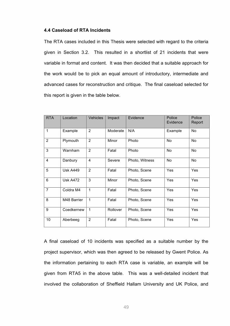
A final caseload of 10 incidents was specified as a suitable number by the
project supervisor, which was then agreed to be released by Gwent Police. As
the information pertaining to each RTA case is variable, an example will be
given from RTA5 in the above table. This was a well-detailed incident that
involved the collaboration of Sheffield Hallam University and UK Police, and
50
also included many of the calculations outlined in the previous chapter. For a
more detail of the evidence, please see Appendix I & II.
4.5 Example of RTA Case Evidence
RTA5: Collision between two vehicles on the A449, Usk, Wales, on 15th
October 2011
The following information is taken as evidence from the final report submitted by
the RTA Investigator (PC Goddard) assigned to the incident.
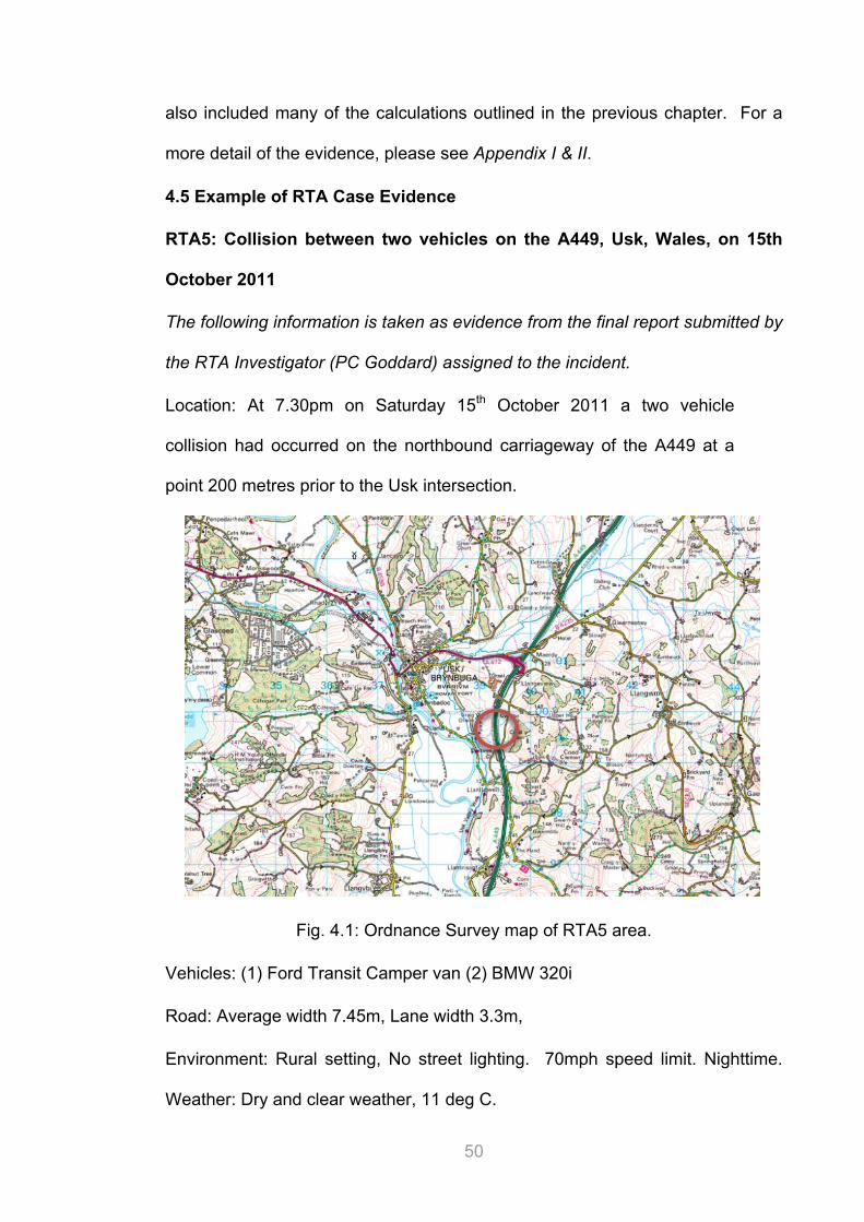
Location: At 7.30pm on Saturday 15th October 2011 a two vehicle
collision had occurred on the northbound carriageway of the A449 at a
point 200 metres prior to the Usk intersection.
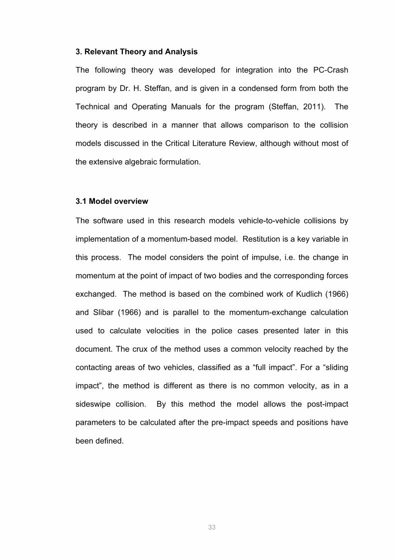
Fig. 4.1: Ordnance Survey map of RTA5 area.
Vehicles: (1) Ford Transit Camper van (2) BMW 320i
Road: Average width 7.45m, Lane width 3.3m,
Environment: Rural setting, No street lighting. 70mph speed limit. Nighttime.
Weather: Dry and clear weather, 11 deg C.
51
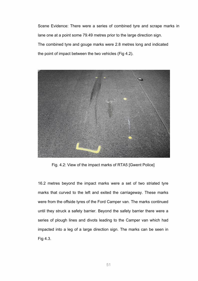
Scene Evidence: There were a series of combined tyre and scrape marks in
lane one at a point some 79.49 metres prior to the large direction sign.
The combined tyre and gouge marks were 2.8 metres long and indicated
the point of impact between the two vehicles (Fig 4.2).
Fig. 4.2: View of the impact marks of RTA5 [Gwent Police]
16.2 metres beyond the impact marks were a set of two striated tyre
marks that curved to the left and exited the carriageway. These marks
were from the offside tyres of the Ford Camper van. The marks continued
until they struck a safety barrier. Beyond the safety barrier there were a
series of plough lines and divots leading to the Camper van which had
impacted into a leg of a large direction sign. The marks can be seen in
Fig 4.3.
52
Fig. 4.3: View showing the camper van’s path of RTA5 [Gwent Police]
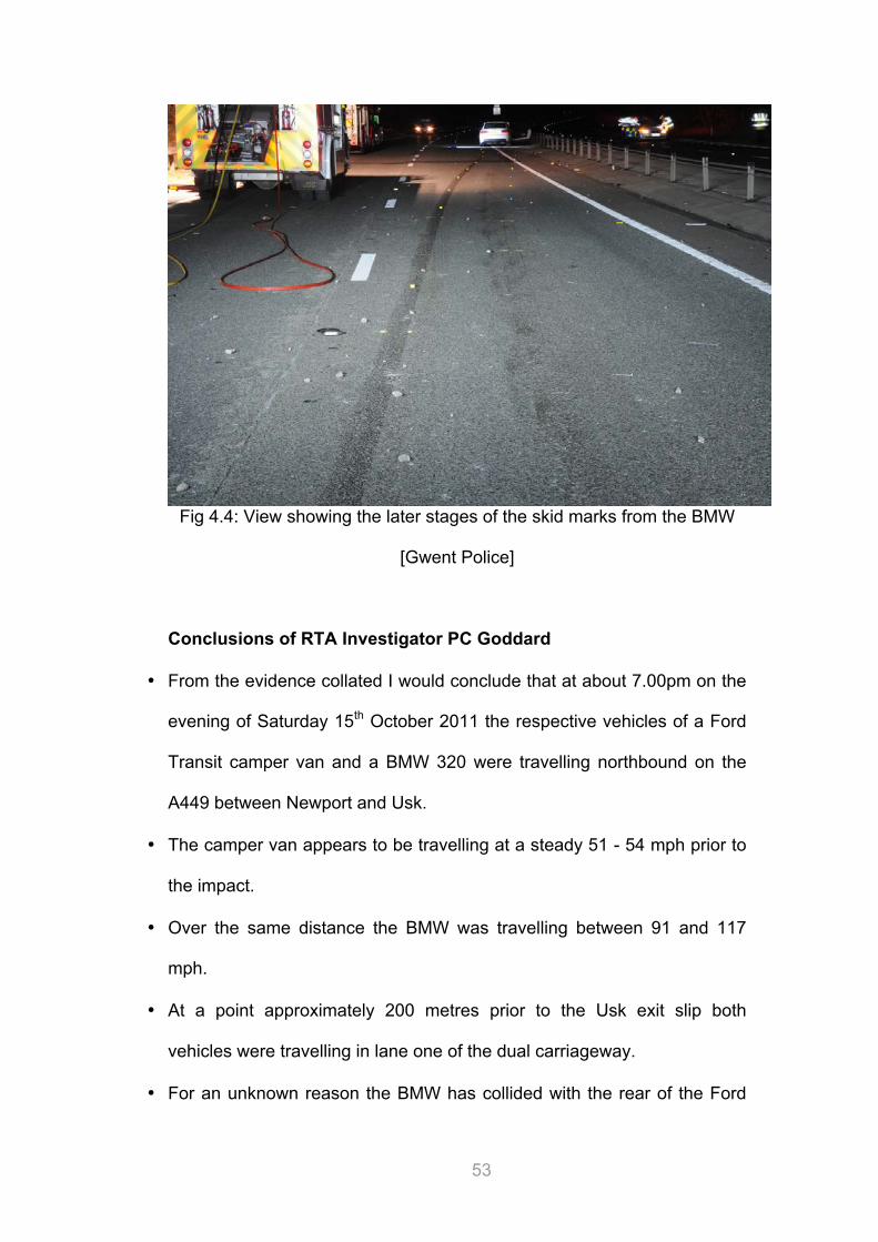
On the centre white line and some 32 metres after the impact a locked tyre
mark started and progressed across lane two for a distance of 81.6 metres
ending under the front nearside tyre of the BMW 320 which was located some
116.5 metres from the point of impact. A second locked tyre mark ran parallel to
the one above for the last 45.5 metres and ended under the front offside tyre of
the BMW (Fig 4.4). The distance from the point of impact to the end of the skid
marks was 116.5 metres.
53
Fig 4.4: View showing the later stages of the skid marks from the BMW
[Gwent Police]
Conclusions of RTA Investigator PC Goddard
• From the evidence collated I would conclude that at about 7.00pm on the
evening of Saturday 15th October 2011 the respective vehicles of a Ford
Transit camper van and a BMW 320 were travelling northbound on the
A449 between Newport and Usk.
• The camper van appears to be travelling at a steady 51 - 54 mph prior to
the impact.
• Over the same distance the BMW was travelling between 91 and 117
mph.
• At a point approximately 200 metres prior to the Usk exit slip both
vehicles were travelling in lane one of the dual carriageway.
• For an unknown reason the BMW has collided with the rear of the Ford
54
Transit.
• If the Ford camper had maintained its progress then the speed of the
BMW at this point would be between 99 and 103 mph.
• A post impact event recorded by one of the BMW’s safety systems
recorded a speed of 87 mph.
• After impact the Ford has veered to the left and collided with a crash
barrier on the nearside verge. The van vaulted the barrier and collided
with the leg of a substantial sign. The driver died at the scene.
• After impact the BMW has veered to the right into lane two. The brakes
have been applied such that the front wheels locked and left skid marks
for 116.55 metres. The speed of the BMW at this point was between 74
and 84 mph.
• With the Ford travelling at 51 mph and the BMW closing to the rear at 99
mph an impact is avoidable until the vehicles are within 27.5 metres
apart.
• With a closing speed of 48 mph (99 – 51mph) between the BMW and the
camper van, the camper van would have been in view for 25 seconds with a
direct line of sight for the last 16 seconds before impact.
55
4.6 Scenario Modelling Methodology
From information given in the above reporting, the modelling scenario will be
constructed primarily from these findings of the RTA Investigator, and combined
with other mapping information to form a virtual environment. This process
typically consists of 3 stages:
• Mapping: Creating an environment representing the scene
• Vehicles & Dynamics: Selecting the most appropriate vehicles and
characteristics, with pre-impact speed and direction
• Impact: Reconstructing the moment of impact in the collision
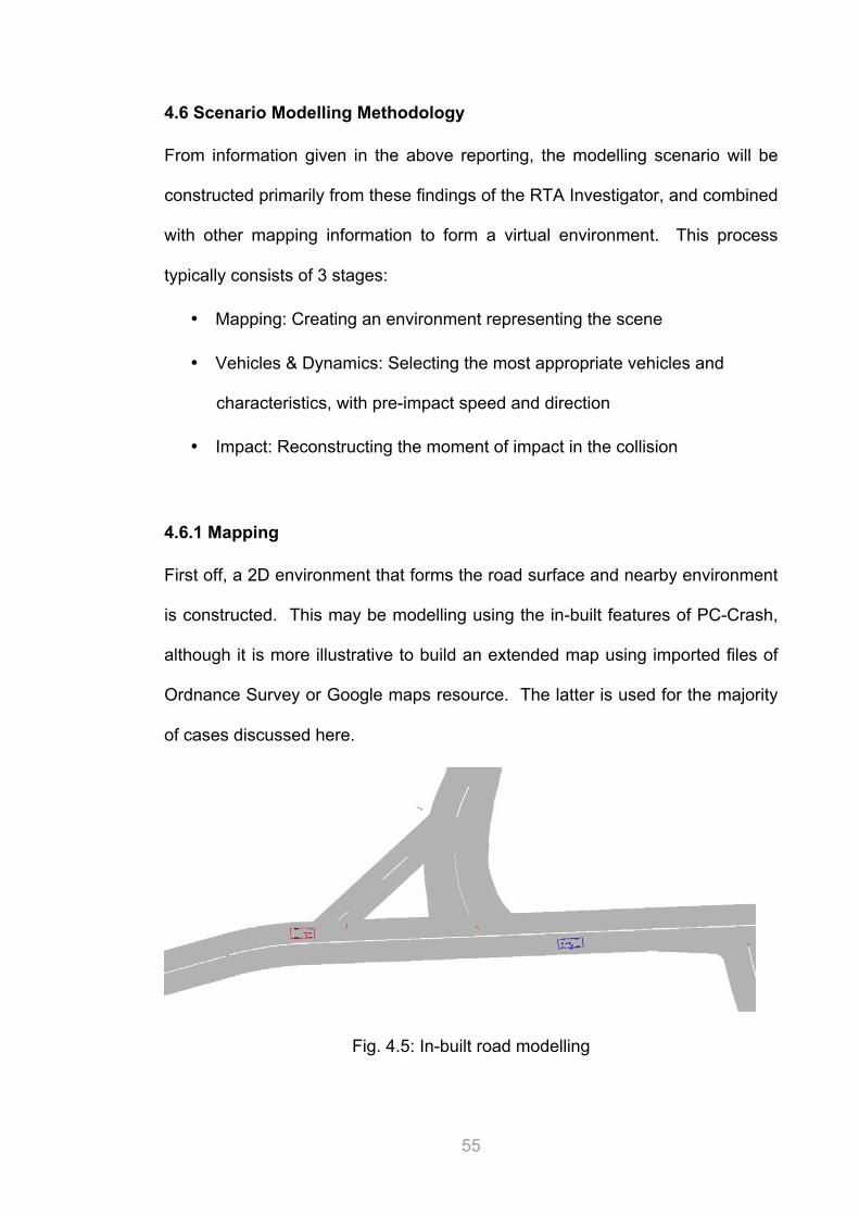
4.6.1 Mapping
First off, a 2D environment that forms the road surface and nearby environment
is constructed. This may be modelling using the in-built features of PC-Crash,
although it is more illustrative to build an extended map using imported files of
Ordnance Survey or Google maps resource. The latter is used for the majority
of cases discussed here.
Fig. 4.5: In-built road modelling
56
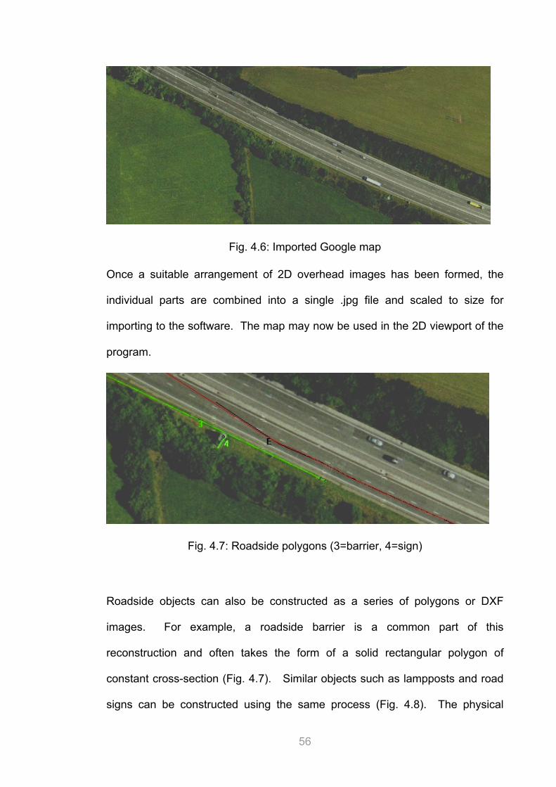
Fig. 4.6: Imported Google map
Once a suitable arrangement of 2D overhead images has been formed, the
individual parts are combined into a single .jpg file and scaled to size for
importing to the software. The map may now be used in the 2D viewport of the
program.
Fig. 4.7: Roadside polygons (3=barrier, 4=sign)
Roadside objects can also be constructed as a series of polygons or DXF
images. For example, a roadside barrier is a common part of this
reconstruction and often takes the form of a solid rectangular polygon of
constant cross-section (Fig. 4.7). Similar objects such as lampposts and road
signs can be constructed using the same process (Fig. 4.8). The physical
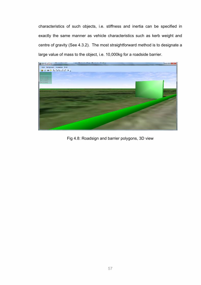
57
characteristics of such objects, i.e. stiffness and inertia can be specified in
exactly the same manner as vehicle characteristics such as kerb weight and
centre of gravity (See 4.3.2). The most straightforward method is to designate a
large value of mass to the object, i.e. 10,000kg for a roadside barrier.
Fig 4.8: Roadsign and barrier polygons, 3D view
58
4.6.2 Vehicle Modelling
The range and scope of cars and other vehicles on the roads means that a
basic, generic model of a car is unsuitable for collision modelling. Fortunately,
the PC Crash program contains a verbose library of vehicles of various types
which can be readily implemented with a few clicks of the mouse. This section
demonstrates how to tailor the specifications, attributes and individual features
of a vehicle in a collision to represent it with the most accuracy. The blocky
appearance of vehicles can be improved by using the 3D models included in
the software.
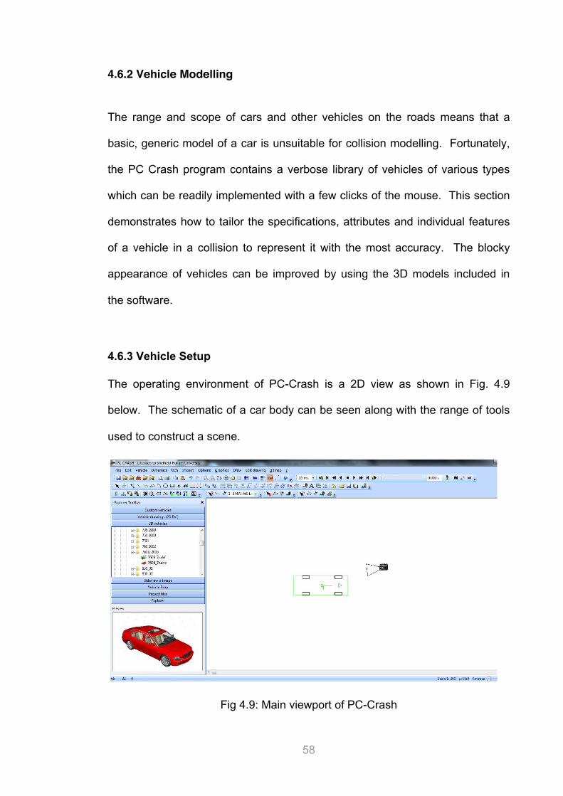
4.6.3 Vehicle Setup
The operating environment of PC-Crash is a 2D view as shown in Fig. 4.9
below. The schematic of a car body can be seen along with the range of tools
used to construct a scene.
Fig 4.9: Main viewport of PC-Crash
59
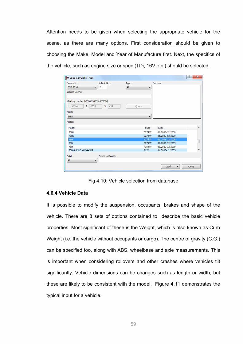
Attention needs to be given when selecting the appropriate vehicle for the
scene, as there are many options. First consideration should be given to
choosing the Make, Model and Year of Manufacture first. Next, the specifics of
the vehicle, such as engine size or spec (TDi, 16V etc.) should be selected.
Fig 4.10: Vehicle selection from database
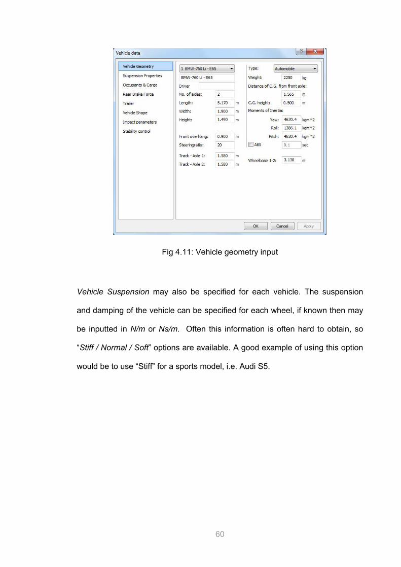
4.6.4 Vehicle Data
It is possible to modify the suspension, occupants, brakes and shape of the
vehicle. There are 8 sets of options contained to describe the basic vehicle
properties. Most significant of these is the Weight, which is also known as Curb
Weight (i.e. the vehicle without occupants or cargo). The centre of gravity (C.G.)
can be specified too, along with ABS, wheelbase and axle measurements. This
is important when considering rollovers and other crashes where vehicles tilt
significantly. Vehicle dimensions can be changes such as length or width, but
these are likely to be consistent with the model. Figure 4.11 demonstrates the
typical input for a vehicle.
60
Fig 4.11: Vehicle geometry input
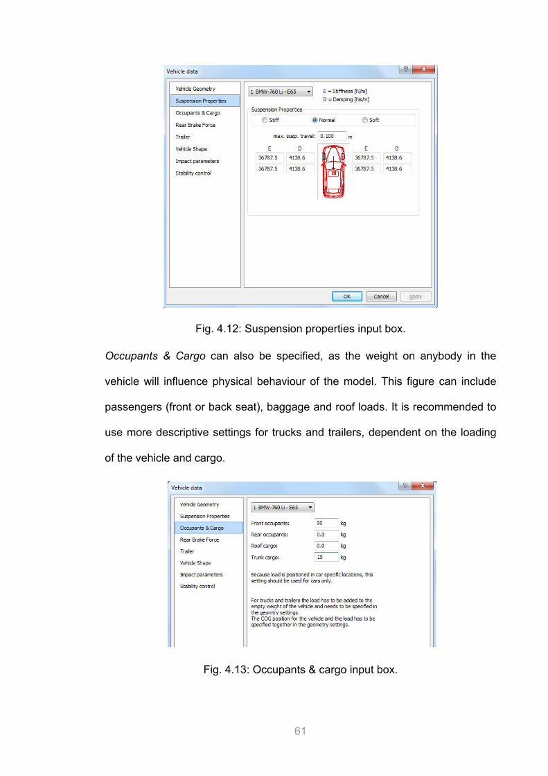
Vehicle Suspension may also be specified for each vehicle. The suspension
and damping of the vehicle can be specified for each wheel, if known then may
be inputted in N/m or Ns/m. Often this information is often hard to obtain, so
“Stiff / Normal / Soft” options are available. A good example of using this option
would be to use “Stiff” for a sports model, i.e. Audi S5.
61
Fig. 4.12: Suspension properties input box.
Occupants & Cargo can also be specified, as the weight on anybody in the
vehicle will influence physical behaviour of the model. This figure can include
passengers (front or back seat), baggage and roof loads. It is recommended to
use more descriptive settings for trucks and trailers, dependent on the loading
of the vehicle and cargo.
Fig. 4.13: Occupants & cargo input box.
62
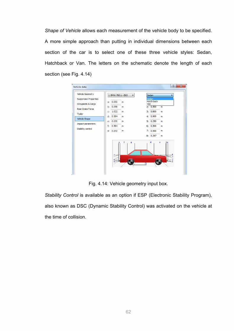
Shape of Vehicle allows each measurement of the vehicle body to be specified.
A more simple approach than putting in individual dimensions between each
section of the car is to select one of these three vehicle styles: Sedan,
Hatchback or Van. The letters on the schematic denote the length of each
section (see Fig. 4.14)
Fig. 4.14: Vehicle geometry input box.
Stability Control is available as an option if ESP (Electronic Stability Program),
also known as DSC (Dynamic Stability Control) was activated on the vehicle at
the time of collision.
63
Fig. 4.15: Stability control input box.
Engine and Drivetrain specifications are also available although not all of these
are used frequently and are not necessary for basic collisions. For example, if a
vehicle in a crash was not accelerating, then the engine options can be kept as
standard. In cases of a vehicle known to be accelerating along a path before a
collision, the power and variables of the engine can be important to the
accuracy of the reconstruction (See Fig. 4.16 below).
Fig. 4.16: Engine & Drivetrain control box.
64
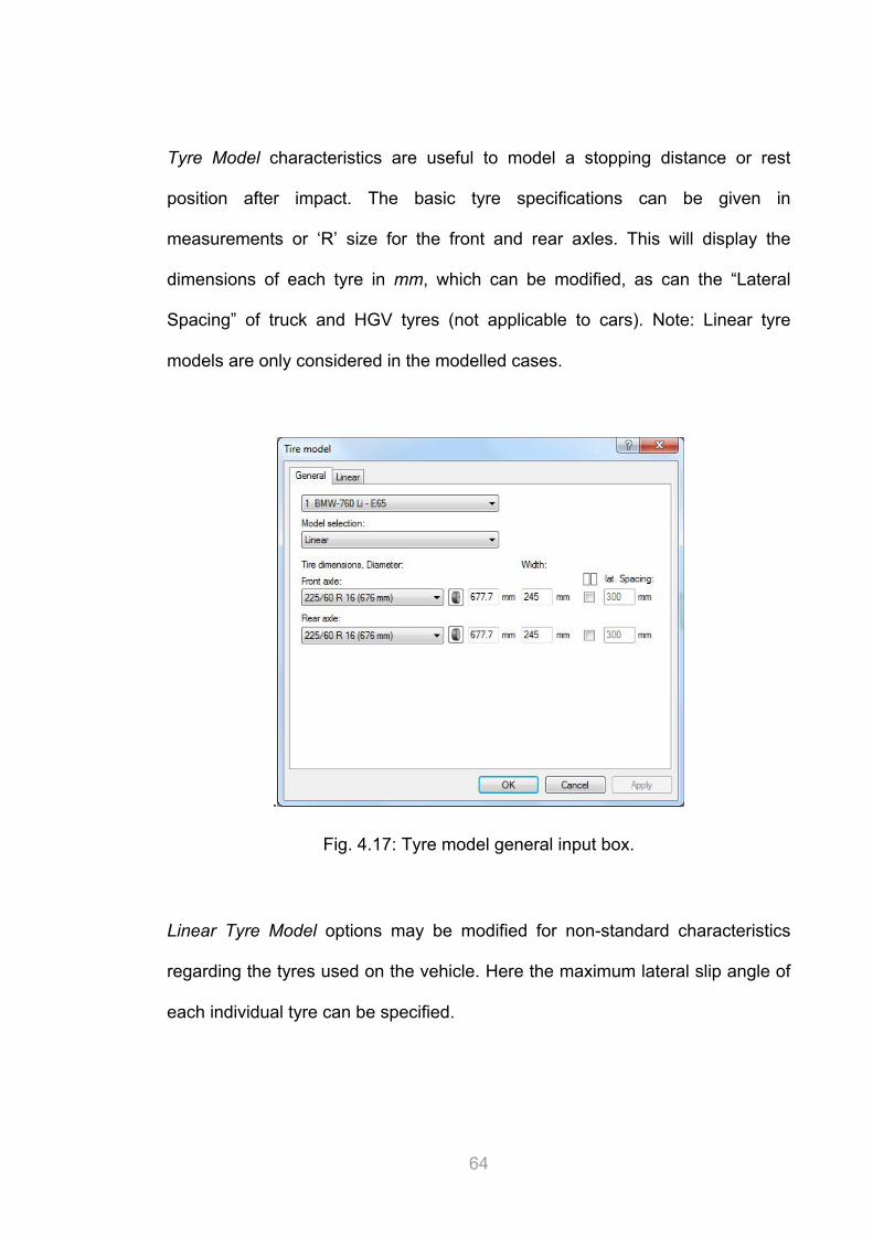
Tyre Model characteristics are useful to model a stopping distance or rest
position after impact. The basic tyre specifications can be given in
measurements or ‘R’ size for the front and rear axles. This will display the
dimensions of each tyre in mm, which can be modified, as can the “Lateral
Spacing” of truck and HGV tyres (not applicable to cars). Note: Linear tyre
models are only considered in the modelled cases.
.
Fig. 4.17: Tyre model general input box.
Linear Tyre Model options may be modified for non-standard characteristics
regarding the tyres used on the vehicle. Here the maximum lateral slip angle of
each individual tyre can be specified.
65
Fig. 4.18: Linear Tyre Model control box.
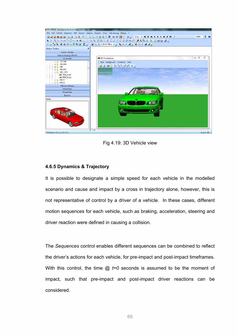
3D Models are of assistance in improving the graphical capabilities of the
software. A vehicle catalogue of DXF files of 3D models can be used to give a
more realistic look to the reconstructions. The figure below shows the
catalogue icon and rendered view for a BMW 760i model. Colours can be
chosen once the file is imported. It should be stated clearly that the DXF files
are a purely graphical input to the program and have no physical influence on
the simulations whatsoever.
66
Fig 4.19: 3D Vehicle view
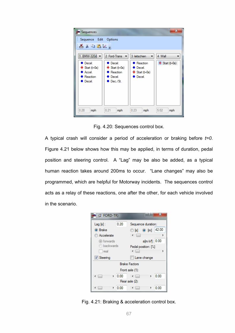
4.6.5 Dynamics & Trajectory
It is possible to designate a simple speed for each vehicle in the modelled
scenario and cause and impact by a cross in trajectory alone, however, this is
not representative of control by a driver of a vehicle. In these cases, different
motion sequences for each vehicle, such as braking, acceleration, steering and
driver reaction were defined in causing a collision.
The Sequences control enables different sequences can be combined to reflect
the driver’s actions for each vehicle, for pre-impact and post-impact timeframes.
With this control, the time @ t=0 seconds is assumed to be the moment of
impact, such that pre-impact and post-impact driver reactions can be
considered.
67
Fig. 4.20: Sequences control box.
A typical crash will consider a period of acceleration or braking before t=0.
Figure 4.21 below shows how this may be applied, in terms of duration, pedal
position and steering control. A “Lag” may be also be added, as a typical
human reaction takes around 200ms to occur. “Lane changes” may also be
programmed, which are helpful for Motorway incidents. The sequences control
acts as a relay of these reactions, one after the other, for each vehicle involved
in the scenario.
Fig. 4.21: Braking & acceleration control box.
68
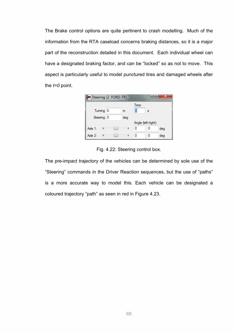
The Brake control options are quite pertinent to crash modelling. Much of the
information from the RTA caseload concerns braking distances, so it is a major
part of the reconstruction detailed in this document. Each individual wheel can
have a designated braking factor, and can be “locked” so as not to move. This
aspect is particularly useful to model punctured tires and damaged wheels after
the t=0 point.
Fig. 4.22: Steering control box.
The pre-impact trajectory of the vehicles can be determined by sole use of the
“Steering” commands in the Driver Reaction sequences, but the use of “paths”
is a more accurate way to model this. Each vehicle can be designated a
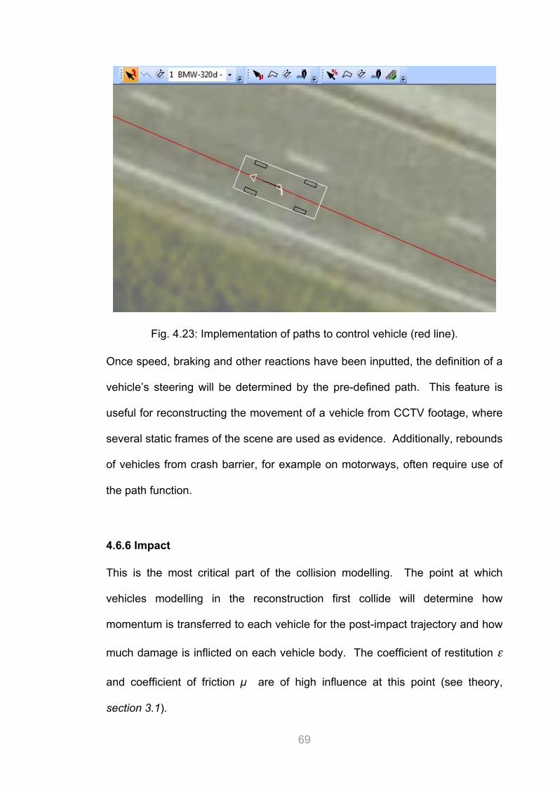
coloured trajectory “path” as seen in red in Figure 4.23.
69
Fig. 4.23: Implementation of paths to control vehicle (red line).
Once speed, braking and other reactions have been inputted, the definition of a
vehicle’s steering will be determined by the pre-defined path. This feature is
useful for reconstructing the movement of a vehicle from CCTV footage, where
several static frames of the scene are used as evidence. Additionally, rebounds
of vehicles from crash barrier, for example on motorways, often require use of
the path function.
4.6.6 Impact
This is the most critical part of the collision modelling. The point at which
vehicles modelling in the reconstruction first collide will determine how
momentum is transferred to each vehicle for the post-impact trajectory and how
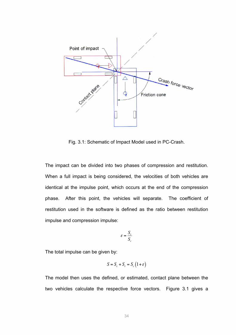
much damage is inflicted on each vehicle body. The coefficient of restitution ε
and coefficient of friction µ are of high influence at this point (see theory,
section 3.1).
70
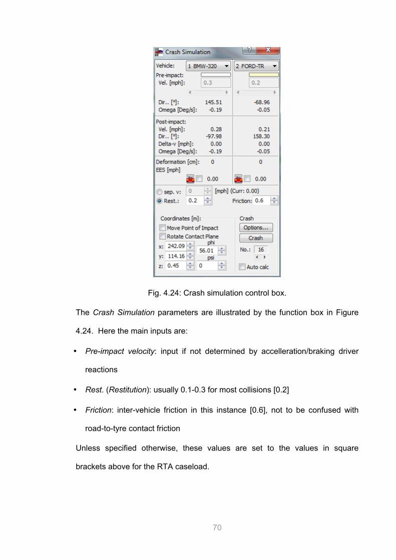
Fig. 4.24: Crash simulation control box.
The Crash Simulation parameters are illustrated by the function box in Figure
4.24. Here the main inputs are:
• Pre-impact velocity: input if not determined by accelleration/braking driver
reactions
• Rest. (Restitution): usually 0.1-0.3 for most collisions [0.2]
• Friction: inter-vehicle friction in this instance [0.6], not to be confused with
road-to-tyre contact friction
Unless specified otherwise, these values are set to the values in square
brackets above for the RTA caseload.
71
For each collision, the Crash Simulation function then determines the Point of
Impact and post impact parameters for each individual impact:
• Post-impact velocity
• Direction of post-impact travel
• Delta-v
• Omega (Yaw or tilt)
• Deformation (in cm or EES)
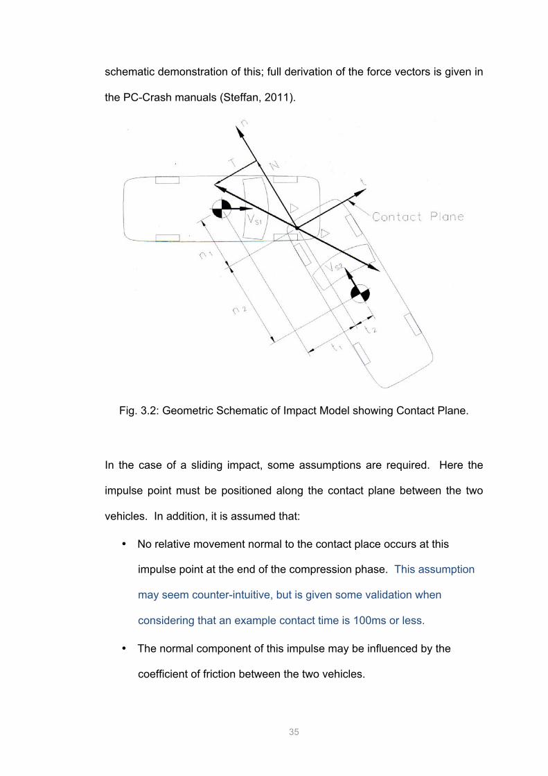
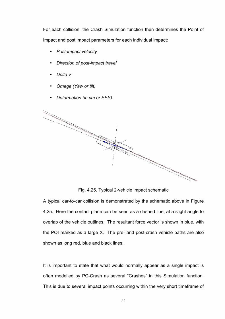
Fig. 4.25. Typical 2-vehicle impact schematic
A typical car-to-car collision is demonstrated by the schematic above in Figure
4.25. Here the contact plane can be seen as a dashed line, at a slight angle to
overlap of the vehicle outlines. The resultant force vector is shown in blue, with
the POI marked as a large X. The pre- and post-crash vehicle paths are also
shown as long red, blue and black lines.
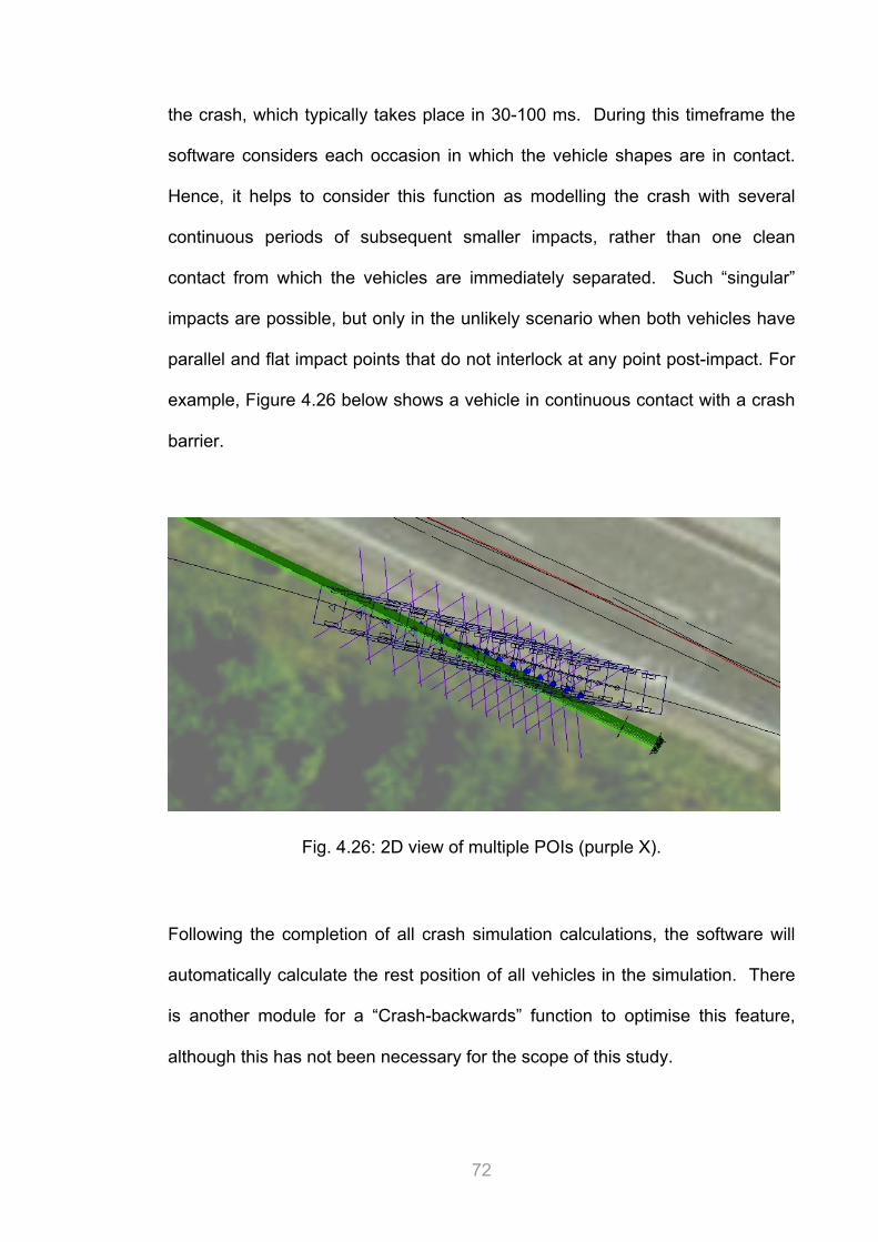
It is important to state that what would normally appear as a single impact is
often modelled by PC-Crash as several “Crashes” in this Simulation function.
This is due to several impact points occurring within the very short timeframe of
72
the crash, which typically takes place in 30-100 ms. During this timeframe the
software considers each occasion in which the vehicle shapes are in contact.
Hence, it helps to consider this function as modelling the crash with several
continuous periods of subsequent smaller impacts, rather than one clean
contact from which the vehicles are immediately separated. Such “singular”
impacts are possible, but only in the unlikely scenario when both vehicles have
parallel and flat impact points that do not interlock at any point post-impact. For
example, Figure 4.26 below shows a vehicle in continuous contact with a crash
barrier.
Fig. 4.26: 2D view of multiple POIs (purple X).
Following the completion of all crash simulation calculations, the software will
automatically calculate the rest position of all vehicles in the simulation. There
is another module for a “Crash-backwards” function to optimise this feature,
although this has not been necessary for the scope of this study.
73
4.7 Accuracy of Evidence
Here some discussion is given to the methods in which police investigators
gather evidence and how accurate these processes are. Cases from Gwent
police form the bulk of this thesis and only incidents from this constabulary will
be discussed here.
On arriving at the scene of an RTA, the police investigator will have multiple
responsibilities. The following discusses what technical evidence is to be
gathered, and how potential loss of accuracy could occur.
Witnesses
The investigator will gather statements from all persons present at the scene.
This may include drivers, passenger, passers-by, local residents and also other
police present at the scene. A brief statement can be taken as notes or audio
which is usually then expanded on in full at the local station. This form of
evidence is not technical, but highly influential; a vocal statement from a person
in court may be powerful in determining a case. The loss of accuracy with this
kind of evidence can be due to anything from memory, to fear, deceit and
shock. Hence this is very hard to quantify in a technical context. For all cases
included in this thesis, witness statements are wholly disregarded for these
reasons.
Measurements
The investigator will then gather a list of RTA measurements required from the
scene. This may include
• Skid marks: obtained with a tape measure or laser device. Accuracy is
dependent on visibility of the marks and the device calibration. Most
measurements in this thesis are given to the nearest metre, providing some
error to each case. It is understood that accuracy is limited more by time
rather than the precision of equipment.
• Vehicle paths: established by observing tyre marks. Plastic ‘markers’ are
placed in the paths and then photographed. This is especially helpful for
74
nighttime incidents. Accuracy is dependent on this skill of the investigator
present. Reconstructing vehicle paths via this method will have resulted in
some inaccuracy, although the start and end points between impacts were
the vital information for simulations. Detail on these areas was abundant
with many photographs, inclusive of measurement information.
• Environmental damage & features: gathered by professional expertise, i.e.
matching marks on a roadside barrier to scratch marks on vehicle bodies.
This is accurate to establish a ‘point of impact’ to a specific vehicle, but the
point in question can be variable to 0.5-1 vehicle lengths. This is an error
which can be easily integrated to the reconstruction. RF: Environmental
objects such as signs, barriers etc. are static and relatively easy to place on
an overhead-view map. Natural environmental objects are variable in size
and position and represent a great difficulty in simulation.
• Weather, temperature, conditions: measured or observed at the scene. A
thermometer or laser temperature device is mostly used to get ambient
conditions, but more importantly, road surface conditions. A digital/laser
thermometer will be typically be accurate to one decimal place. These
measurements are influential to tyre-road friction and given strong concern.
Combined with information from weather reports, data in this field is typically
accurate.
• Visibility, Daylight, Street lighting: a matter of observation, thus somewhat
subjective. However the time of the incident will be carefully noted, allowing
sunlight and weather data to be retrieved later. The subjective nature of the
visibility status on the ground at the time (or some time after) of the incident
could benefit from greater accuracy. For example, a foggy morning may be
described as ‘light fog’ or ‘low visibility’ depending on the investigator
present. Such conditions dramatically influence the driving conditions prior
to the incident and can be a source of error regarding incidents.
Vehicles
It is routine to photograph any vehicles in situ and perform more detailed
analysis at another location. The caseload indicated that the following
measurements were performed as standard:
75
• Model, working order, modifications, MOT, overall condition: obtained by a
police garage and records check. The main purpose is to ascertain if all UK
vehicle standards were met before the incident and that the car was in a
roadworthy condition. The accuracy of establishing this depends on the staff
in question, as inspecting a damaged vehicle requires some forensic skill.
• Vehicle damage & crush: an important method for determining the POI and
pre-impact velocity. This may included vehicle-to-vehicle and nearby object
impacts. Some expertise is again required, although crush damage
measurements are commonly made with a standard tape measure to the
nearest cm. This was a large source of error influential to the reconstructed
simulations.
• Tyres: tread remaining will be measured with a gauge (to 0.1mm accuracy)
and inflation pressure can be either be measured or estimated from the
profile and wear. Typically this falls within a legal/nonlegal category.
Underinflated tyres are an often overlooked cause of incidents due to the
increase of braking distance and loss of control.
• Lights: the use and activation of vehicle lights at the POI can be accurately
assessed using a specialist technique. The filament of the bulb can be
studied to ascertain whether each light was off or on at the moment of
impact. An activated brake light, for example, would show a stretched ‘loop
filament’ for a low-speed impact and a ‘hot break’ for a high-speed impact.
Likewise, a unactivated light would show a ‘cold break’ of the filament. The
process is reliable and has been used in court several times, although is
thoroughly ineffective for LED lighting.
• Vehicle computer units: recent and more sophisticated vehicle technologies
allow the unit computer to be taken out and connected. Here a wealth of
data can be extracted, e.g. speed at impact, emergency braking, vehicle
warning systems. This information has the highest degree of accuracy.
After all settings were integrated to the software, an initial reconstruction would
be prepared for criticism (as shown in Chapter 5.)
76
4.8 Integrating Investigator’s Data & Accuracy in Reconstruction
Part of the skill of an RTA investigator’s job is to balance all the available
information and form a firm conclusion about the incident. This is a complex
task due to the multiple forms of evidence and respective accuracies.
For these reasons, the process of reconstruction is often based on a
hypothesis. The most likely pre-crash scenario would be assessed and used
for a trial reconstruction. The evidence would be integrated (as described in
Section 3.2) and an initial reconstruction would then simulate the POI, vehicle
trajectories, and rest positions.
From this point, all measurement errors from the evidence gathered would be
used to refine the process. A good, common example is moving the POI; if
such a point was in the middle of a road, the accuracy may be 0.5m in any
direction. The software allows trajectories and rest positions of vehicles to be
assessed in real-time as the POI is moved. The same principle is true of
vehicle speeds, allowing the scenario to be improved significantly using these
means.
Secondary refinements would typically adjust reconstruction variables such as
vehicle-to-vehicle contact angle, friction, and restitution settings. These values
are all either automatically calculated or set as default in the software, and
adjustment of these helps to define the characteristics of the impact.
Subsequent adjustments would involve surface friction to compensate for
weather conditions. Road friction is commonly measured at a coefficient of 0.7-
0.9, although for wet and icy conditions this will drop. Other subsequent
changes made would be vehicle settings, for example centre of gravity,
occupants and loading, and perhaps tyre settings (e.g. for underinflated or worn
tyres), although no tyre adjustments were required for the caseload
demonstrated here.
77
Overall the most commonly adjusted settings in the caseload studied consisted
of:
• Vehicle-to-vehicle restitution
• Vehicle-to-vehicle friction
• Road/surface friction
• Point of Impact
• Contact Angle / Angle of Impact
It is noted that the adjustment of these settings deserves further discussion to
the effect of the reconstruction process. Such discussion is continued in
Chapter 6.
78
5. Results
In this chapter, the initial modelling of the RTA caseload is presented. Each
incident was reconstructed using the maximum possible amount of available
evidence, together with the methods described in the previous chapters. It is
important to state that only police reporting and evidence was used at this
point; this allows for RTA Investigators to view the reconstructions and
provide a critique of the process and its accuracy for the following chapters.
Each RTA casefile here is presented in this document as a series of “contact
sheet” slideshow images that describe the 3D reconstruction. Full evidence
is given in the appendices of this document, although full video files of each
reconstruction are available via a public shared folder (See Appendix A).
This folder is recommended for a first viewing of the caseload, and will be
available for 12 months after the submission date of this document.
Commentaries
Where evidence and commentary on each incident has been provided, the
source of the information is given with regard to:
• Public: Newspapers, reports and non-private sources
• GP: Private domain information from Gwent Police
• SJU: Opinions and conclusions of the author.
Please note all velocity and damage are software-calculated unless specified
otherwise.
79
5.1 RTA1 Collision: Car rear end shunt (example)
Study: This example serves to illustrate the general operation and interface
of the PC-Crash collision software.
Scenario: A basic setup is described where two cars collide.
In this instance, Car 1 is travelling at 30 km/h in a straight line, directly
towards Car 2 which is stationary. Both cars are VW Golfs, MK5 1.6
versions. Brakes are not employed on either car. Here the restitution
between the vehicles causes the motion of stopping.
Figure 5.1(i): 2-Car Example
Outcome [SJU]: The momentum is transferred between the two identical
vehicles. The point of impact is slightly off-centre as the cars are not
perfectly parallel. This causes the plane of contact between the two cars to
be at an angle to the vertical, although this discrepancy is not of large
80
enough magnitude to be visible in the 3D representation. Deformation to
each car body = 5cm.
RTA1 Slideshow
Figure 5.1 (ii-viii): 2-Car Example
3D side view of the two vehicles. Car 1 (Red) is at speed. The 2D view shows the point of impact (POI) as a purple X and the contact plane as a dashed line [SJU].
On impact, car 1 contacts the rear of car 2. The grey rectangle (in 3D view) marks the POI of a collision [SJU].
The momentum from Car 1 is transferred to Car 2, with both vehicles coming to rest. Note that vehicle damage is not displayed on any view or schematics [SJU].
81
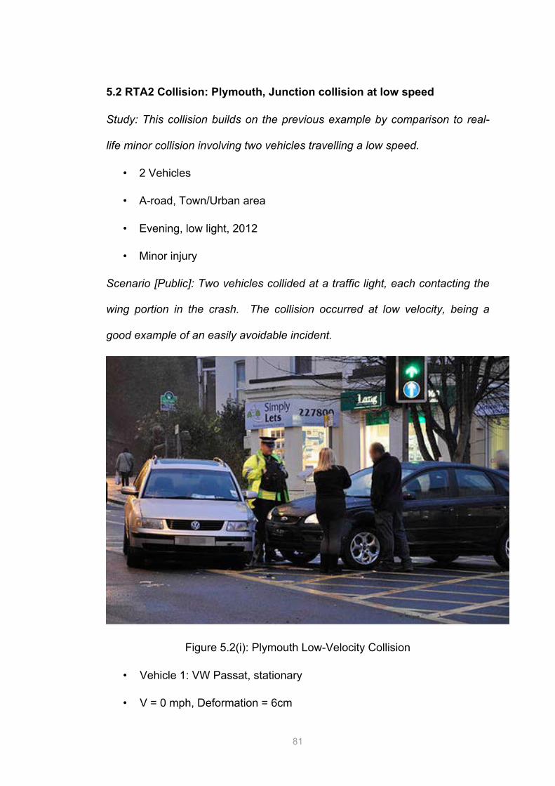
5.2 RTA2 Collision: Plymouth, Junction collision at low speed
Study: This collision builds on the previous example by comparison to real-
life minor collision involving two vehicles travelling a low speed.
• 2 Vehicles
• A-road, Town/Urban area
• Evening, low light, 2012
• Minor injury
Scenario [Public]: Two vehicles collided at a traffic light, each contacting the
wing portion in the crash. The collision occurred at low velocity, being a
good example of an easily avoidable incident.
Figure 5.2(i): Plymouth Low-Velocity Collision
• Vehicle 1: VW Passat, stationary
• V = 0 mph, Deformation = 6cm
82
• Vehicle 2: Ford Focus, braking
• V = 15 mph, Deformation = 8cm
Outcome [SJU]: This case gives an elementary example of how vehicle
motion and mild impact are modelled. First of all, the Passat comes to the
junction, braking to a stop and turning. The area of the box junction is
designated in yellow. Secondly, the Focus approaches the same junction
from an adjoining road, performing the same manoeuvre but failing to notice
the other car.
The Focus then impacts the Passat on the passenger side wing, causing a
minor impact at a 45 degree angle to both cars. Both vehicles are moved
from their initial positions slightly by the impact.
This is a lighter case compared to the other RTA incidents, but nevertheless,
such minor accidents are common and are the cause of many costly
proceedings which can be brought into the judicial systems for negotiation.
3D ground view of the two vehicles. Car 1 (Red) is at speed and approaching the box junction area in yellow, with the POIs and contact plane in the middle of the junction. The 2D view shows the start and rest position of the red car [SJU].
Car 1 slows down to turn in the junction, coming to the POI and contact plane. Car 2 (blue) approaches at a greater speed. The 2D view shows the start and rest position of both vehicles at the junction [SJU].
The momentum from Car 2 causes a minor impact and deflection of Car 1, producing an 2nd POI and contact plane as the vehicle bodies move. The 2D view shows the POIs more clearly and also the small deflection to the left of Car 2 [SJU].
84
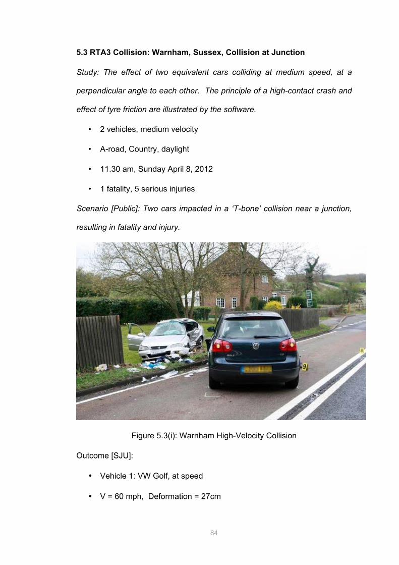
5.3 RTA3 Collision: Warnham, Sussex, Collision at Junction
Study: The effect of two equivalent cars colliding at medium speed, at a
perpendicular angle to each other. The principle of a high-contact crash and
effect of tyre friction are illustrated by the software.
• 2 vehicles, medium velocity
• A-road, Country, daylight
• 11.30 am, Sunday April 8, 2012
• 1 fatality, 5 serious injuries
Scenario [Public]: Two cars impacted in a ‘T-bone’ collision near a junction,
resulting in fatality and injury.
Figure 5.3(i): Warnham High-Velocity Collision
Outcome [SJU]:
• Vehicle 1: VW Golf, at speed
• V = 60 mph, Deformation = 27cm
85
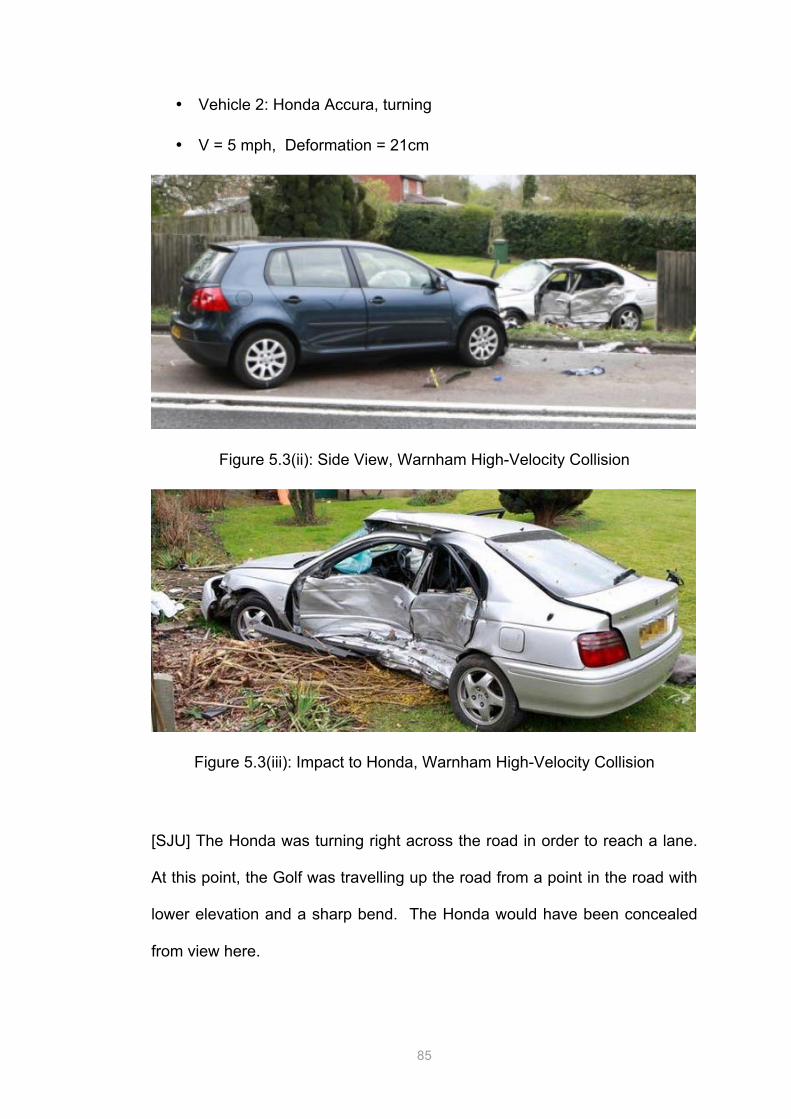
• Vehicle 2: Honda Accura, turning
• V = 5 mph, Deformation = 21cm
Figure 5.3(ii): Side View, Warnham High-Velocity Collision
Figure 5.3(iii): Impact to Honda, Warnham High-Velocity Collision
[SJU] The Honda was turning right across the road in order to reach a lane.
At this point, the Golf was travelling up the road from a point in the road with
lower elevation and a sharp bend. The Honda would have been concealed
from view here.
86
The Golf then collided with the Honda at a right angle, causing high crush to
the side body of the Honda, and causing the vehicles to both move along the
path of the road. Tyre marks were left by both cars. The braking of the Golf
and friction from the tyres of the Honda caused some deceleration, but was
not sufficient to stop the cars. The momentum of the crash then caused the
body of the Honda to rotate anticlockwise before passing over a narrow
grass verge and into a garden fence. The braking action of the Golf stopped
this car in the lefthand lane of the road.
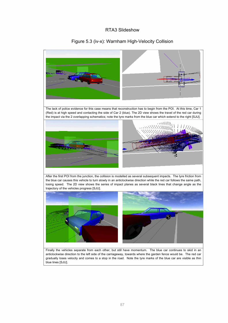
The available evidence for this collision consists of a series of photos with no
witness, news or RTA statements. Nevertheless, the crush damage, rest
positions and tyre marks can still be used to obtain a reconstruction of the
The lack of police evidence for this case means that reconstruction has to begin from the POI. At this time, Car 1 (Red) is at high speed and contacting the side of Car 2 (blue). The 2D view shows the travel of the red car during the impact via the 2 overlapping schematics; note the tyre marks from the blue car which extend to the right [SJU].
After the first POI from the junction, the collision is modelled as several subsequent impacts. The tyre friction from the blue car causes this vehicle to turn slowly in an anticlockwise direction while the red car follows the same path, losing speed. The 2D view shows the series of impact planes as several black lines that change angle as the trajectory of the vehicles progress [SJU].
Finally the vehicles separate from each other, but still have momentum. The blue car continues to skid in an anticlockwise direction to the left side of the carriageway, towards where the garden fence would be. The red car gradually loses velocity and comes to a stop in the road. Note the tyre marks of the blue car are visible as thin blue lines [SJU].
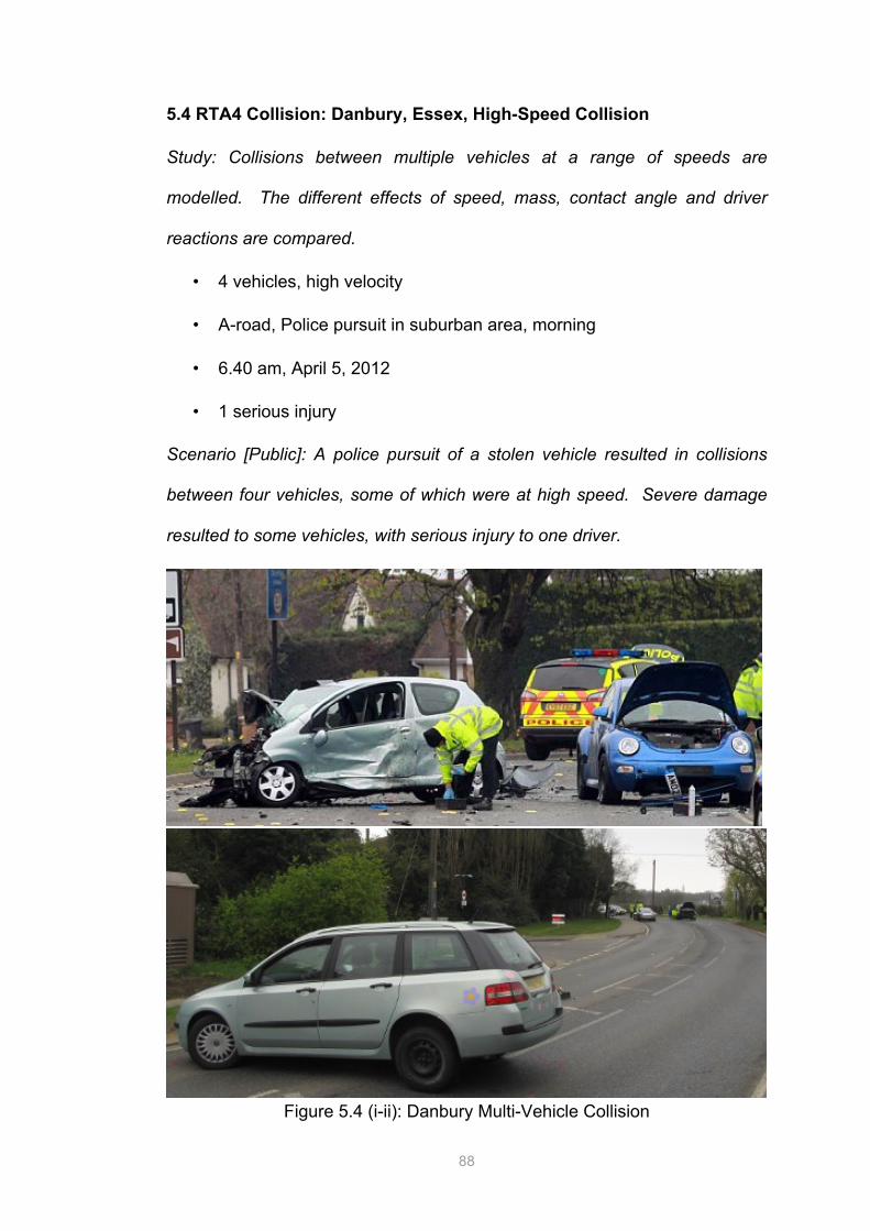
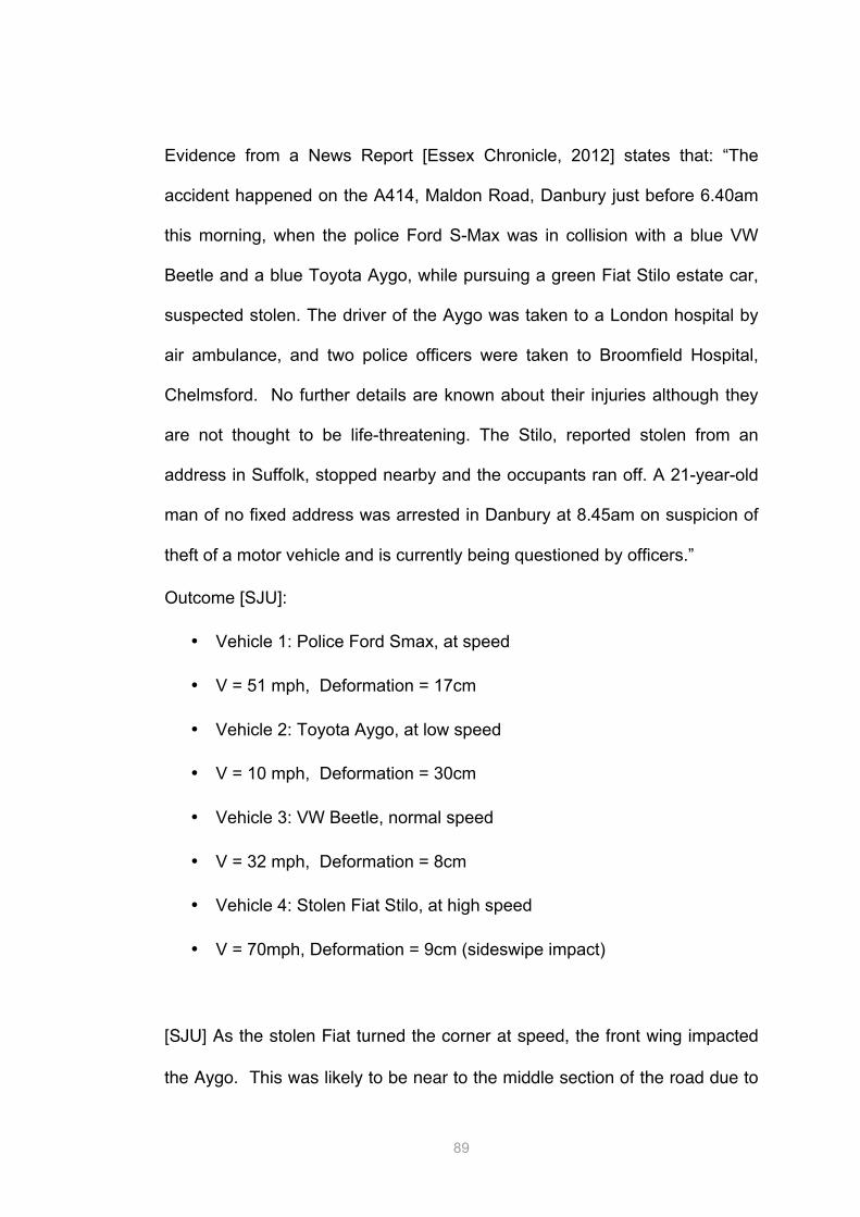
The number of vehicles in this case mean that an extended description is necessary. In the first instance, the grey car (Stolen Fiat Stilo) is travelling at high speed round a bend towards the blue car (Toyota Aygo). The blue car is travelling in the right position in the road although the grey car has drifted across the middle section.
The grey car collides with the blue car on the front right wing section; note the oblique contact plane visible in the overhead 2D view. At this point the green car (VW Beetle) follows behind the blue car, making an avoidance move towards the curb.
At this point, the green car shunts the blue car from behind, causing the green car to stop by the side of the road. This shunt, combined with the previous collision, causes the blue car to divert into the middle of the road. An imminent collision with the upcoming police pursuit car, following the stolen vehicle, is next to occur.
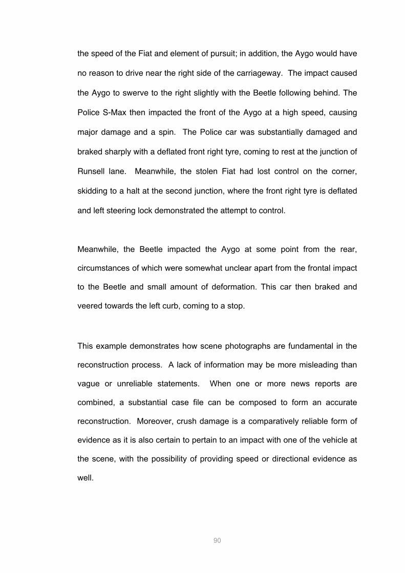
The deviation of both the police and blue cars from their respective sides of the road means that the front of the two vehicles collide in a near head-on fashion; note the impact plane is perpendicular to the direction of travel. This is the most serious impact in this case and is responsible for severe damage to the blue car.
The blue car is spun around by the impact and comes to a stop. The trajectory of this car can be seen by the tyre marks in the overhead 2D view, as can the direction of the police car which comes to a more controlled stop to the left hand side of the road.
The police car comes to a rest within sight of the stolen grey car, which has also come to a stop by the next road junction. The high speed at which the grey car was driven caused a punctured front tyre and resulting loss of control. No further impacts were reported from this point in the incident.
93
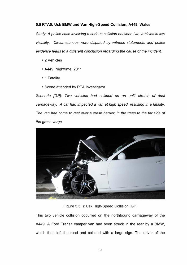
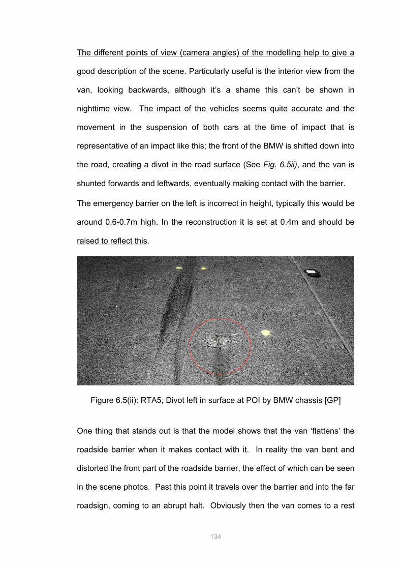
5.5 RTA5: Usk BMW and Van High-Speed Collision, A449, Wales
Study: A police case involving a serious collision between two vehicles in low
visibility. Circumstances were disputed by witness statements and police
evidence leads to a different conclusion regarding the cause of the incident.
• 2 Vehicles
• A449, Nighttime, 2011
• 1 Fatality
• Scene attended by RTA Investigator
Scenario [GP]: Two vehicles had collided on an unlit stretch of dual
carriageway. A car had impacted a van at high speed, resulting in a fatality.
The van had come to rest over a crash barrier, in the trees to the far side of
the grass verge.
Figure 5.5(i): Usk High-Speed Collision [GP]
This two vehicle collision occurred on the northbound carriageway of the
A449. A Ford Transit camper van had been struck in the rear by a BMW,
which then left the road and collided with a large sign. The driver of the
94
camper van was certified dead at the scene. It was alleged that the rear
lights of the camper van were not illuminated, an important matter as this
stretch of road had no streetlights.
Figure 5.5(ii): Usk High-Speed Collision [GP]
Figure 5.5(iii): Usk High-Speed Collision [GP]
95
Figure 5.5(iv): Front of impacted BMW [GP]
Figure 5.5(v): Above view of van in rest position & sign [GP]
96
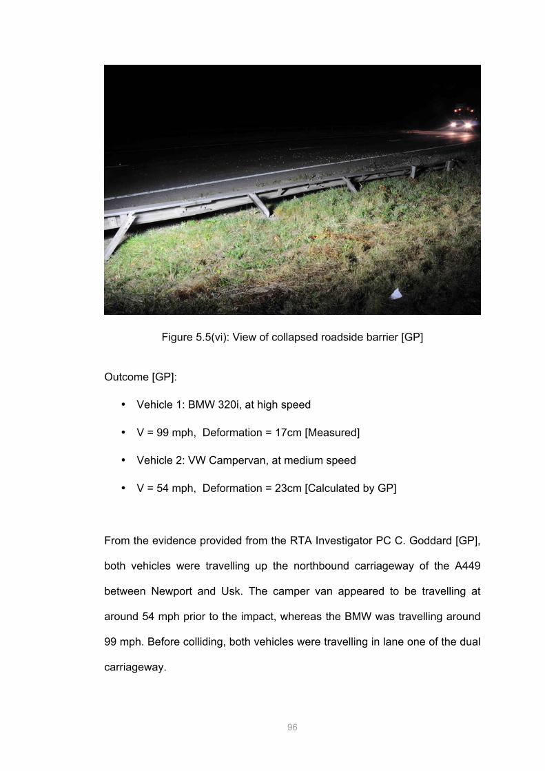
Figure 5.5(vi): View of collapsed roadside barrier [GP]
Outcome [GP]:
• Vehicle 1: BMW 320i, at high speed
• V = 99 mph, Deformation = 17cm [Measured]
• Vehicle 2: VW Campervan, at medium speed
• V = 54 mph, Deformation = 23cm [Calculated by GP]
From the evidence provided from the RTA Investigator PC C. Goddard [GP],
both vehicles were travelling up the northbound carriageway of the A449
between Newport and Usk. The camper van appeared to be travelling at
around 54 mph prior to the impact, whereas the BMW was travelling around
99 mph. Before colliding, both vehicles were travelling in lane one of the dual
carriageway.
97
The BMW then impacted with the rear of the Ford Transit. Extracted
evidence from the BMW computer showed that a post impact event recorded
by one of the safety systems recorded a speed of 87 mph.
The impact caused the Ford to veer left and collide with a crash barrier on
the nearside verge, vaulting the barrier and colliding with the leg of a large
roadsign. Unfortunately the driver of the van died at the scene.
After this impact the BMW veered rightwards into lane two, applying braking
such that the front wheels locked and left skid marks for 116m. Before the
impact, the closing speed between the BMW and the camper van would have
been 48mph, plus the camper van would have been in view for 25 seconds
with a direct line of sight for the last 16 seconds before the impact.
This specific case demonstrates how the information supplied from the RTA
investigator is most helpful in its reconstruction. The scene may be modelled
quickly with a high degree of accuracy to vehicle movement and velocity,
enabling matters such as crush damage and barrier impacts to be focused
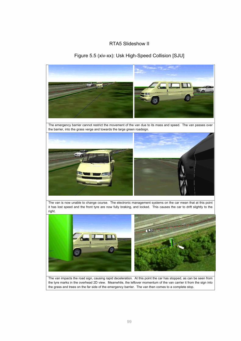
This reconstruction begins from immediately before the impact. The yellow van (VW Camper) is travelling at 55mph along a dual carriageway, with the white car (BMW) approaching swiftly behind at approximately 90mph. Note from the overhead 2D view that the paths overlap closely.
The car makes a rear impact with the van, causing the suspension of both vehicles to change dramatically and alter course of the van. The transfer of kinetic energy from the car means that the van is shunted to the left hand barrier side of the road and increases speed, whereas the car itself loses speed and performs an emergency stop in a forward direction.
The van loses control and veers leftwards; note the altered suspension state. After crossing the carriageway the van makes contact with the emergency barrier running alongside the road, past a green road sign to the side of the trees.
The emergency barrier cannot restrict the movement of the van due to its mass and speed. The van passes over the barrier, into the grass verge and towards the large green roadsign.
The van is now unable to change course. The electronic management systems on the car mean that at this point it has lost speed and the front tyre are now fully braking, and locked. This causes the car to drift slightly to the right.
The van impacts the road sign, causing rapid deceleration. At this point the car has stopped, as can be seen from the tyre marks in the overhead 2D view. Meanwhile, the leftover momentum of the van carrier it from the sign into the grass and trees on the far side of the emergency barrier. The van then comes to a complete stop.
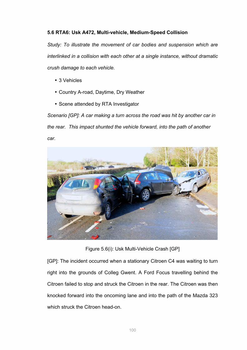
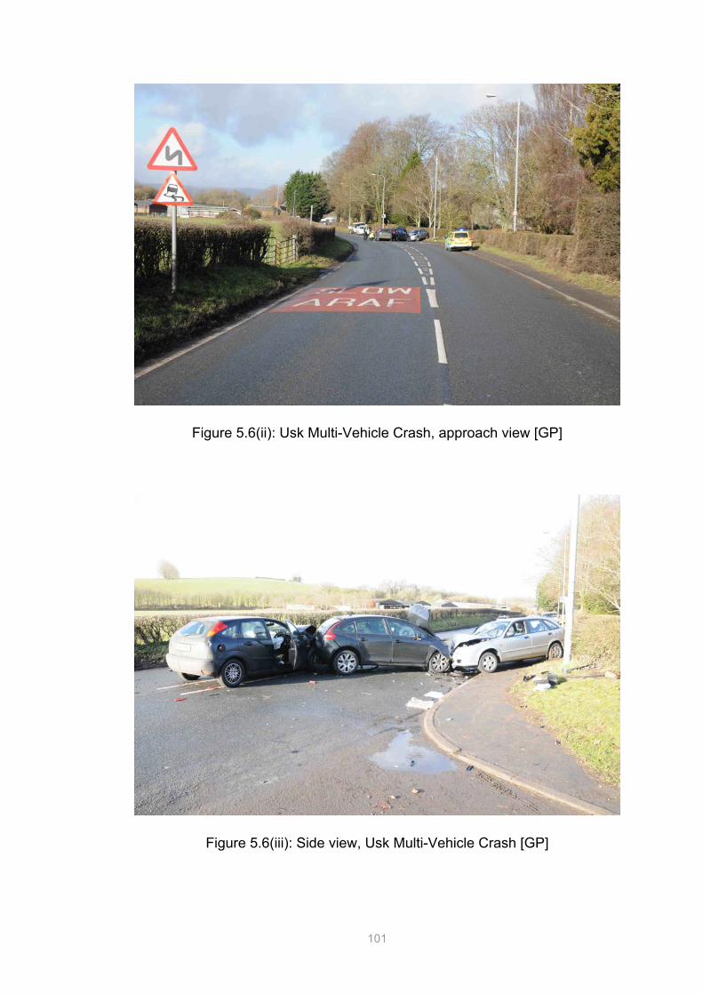
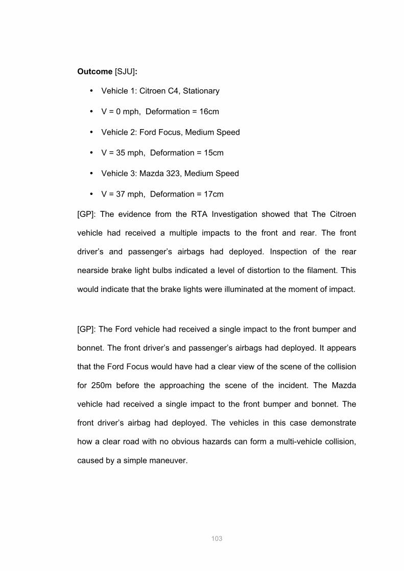
[GP]: The evidence from the RTA Investigation showed that The Citroen
vehicle had received a multiple impacts to the front and rear. The front
driver’s and passenger’s airbags had deployed. Inspection of the rear
nearside brake light bulbs indicated a level of distortion to the filament. This
would indicate that the brake lights were illuminated at the moment of impact.
[GP]: The Ford vehicle had received a single impact to the front bumper and
bonnet. The front driver’s and passenger’s airbags had deployed. It appears
that the Ford Focus would have had a clear view of the scene of the collision
for 250m before the approaching the scene of the incident. The Mazda
vehicle had received a single impact to the front bumper and bonnet. The
front driver’s airbag had deployed. The vehicles in this case demonstrate
how a clear road with no obvious hazards can form a multi-vehicle collision,
caused by a simple maneuver.
104
RTA6 Slideshow I
Figure 5.6 (vi-xi): Usk Multi-Vehicle Crash [SJU]
Imminently before the collision, the Citroen is slowing to a halt to turn right across the road. As this vehicle comes to a stop with some right steering lock, the other two cars approach front the rear and front respectively.
The Focus, directly behind the Citroen, makes contact with the bumper. This impact pushes the Citroen forward and onto the opposite carriageway. The oncoming Mazda in the other side of the road is now in the path of the Citroen. Contact is made when the Citroen is at a 40 degree angle to the median road line.
At the end of the impact, all vehicles are in contact. The Citroen is shunted further forward, and thus pushed the Mazda back into the grass verge. Past this point, all vehicles come to a rest but remain within contact with each other.
From the point of view of the Mazda in the oncoming lane: Imminently before the collision, there is no reason to suspect an accident is about to occur. As the distance between the cars decreases, it becomes evident that the Focus will not halt or evade impact with the Citroen.
The Citroen can now be seen to be proceeding across the median point of the road, with some right steering lock. Note that the rear impact from the Focus moves the Citroen’s suspension down at the front passenger side.
As contact is made with the front bumper of the Mazda and Citroen, the Mazda spins round from the angle of contact of the two vehicles and the sudden deceleration. Note that at this point in the impact, the suspension of the Focus has caused it to yaw to the passenger side.
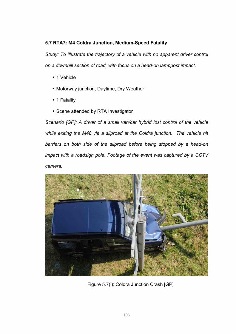
Study: To illustrate the trajectory of a vehicle with no apparent driver control
on a downhill section of road, with focus on a head-on lamppost impact.
• 1 Vehicle
• Motorway junction, Daytime, Dry Weather
• 1 Fatality
• Scene attended by RTA Investigator
Scenario [GP]: A driver of a small van/car hybrid lost control of the vehicle
while exiting the M48 via a sliproad at the Coldra junction. The vehicle hit
barriers on both side of the sliproad before being stopped by a head-on
impact with a roadsign pole. Footage of the event was captured by a CCTV
camera.
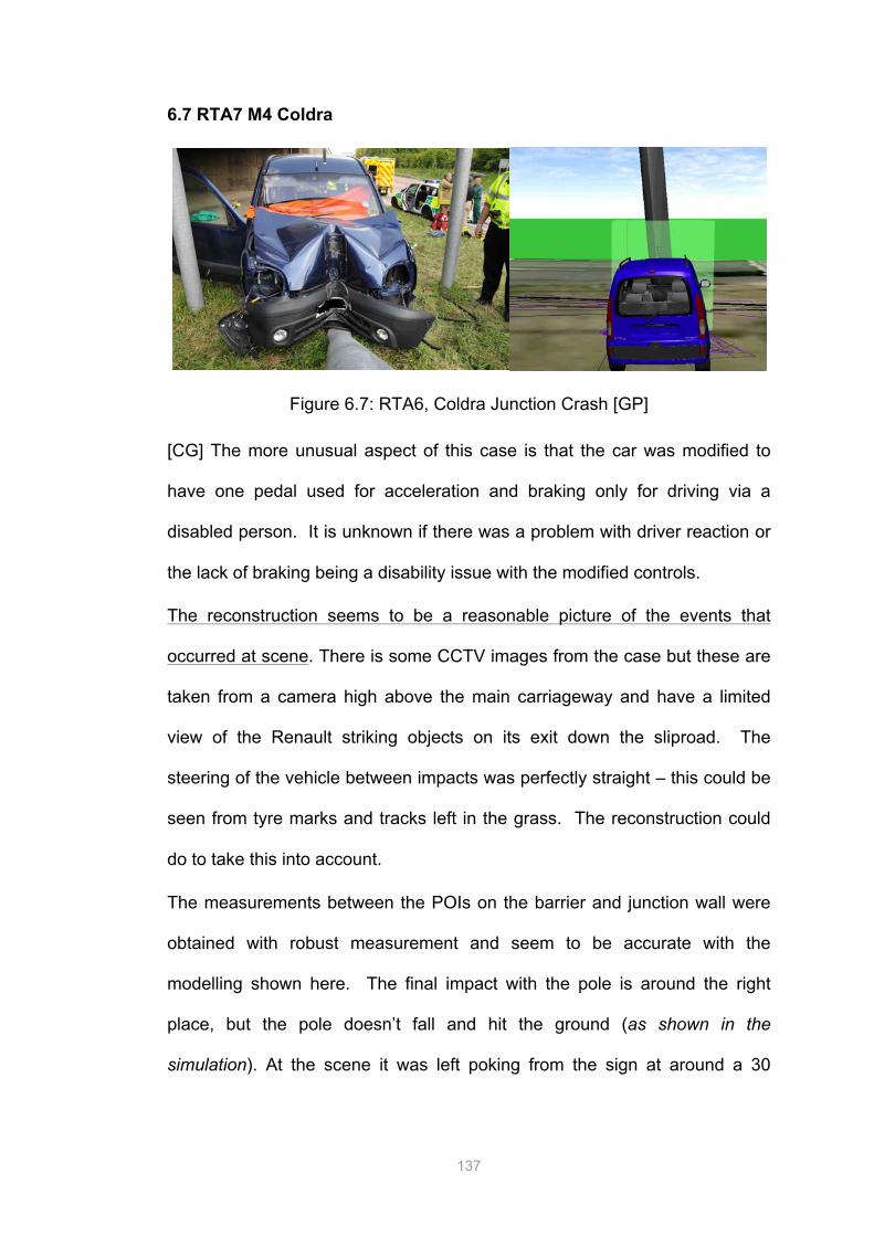
Figure 5.7(i): Coldra Junction Crash [GP]
107
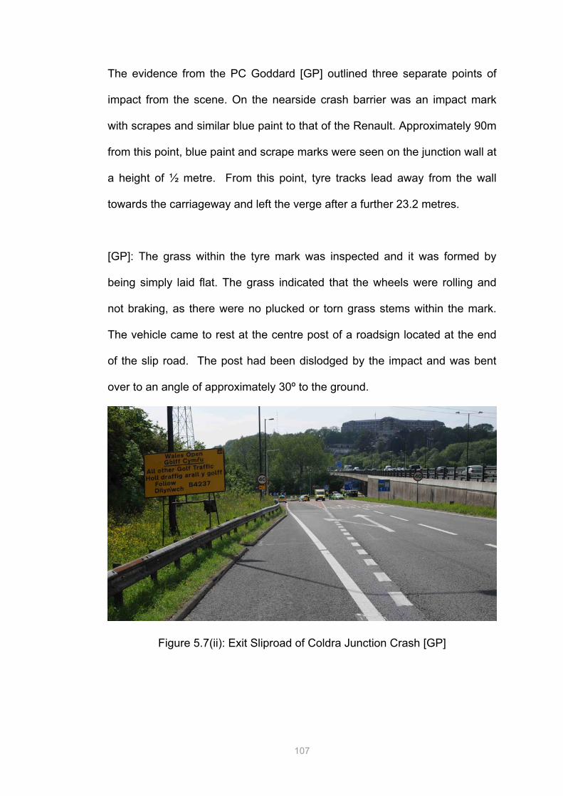
The evidence from the PC Goddard [GP] outlined three separate points of
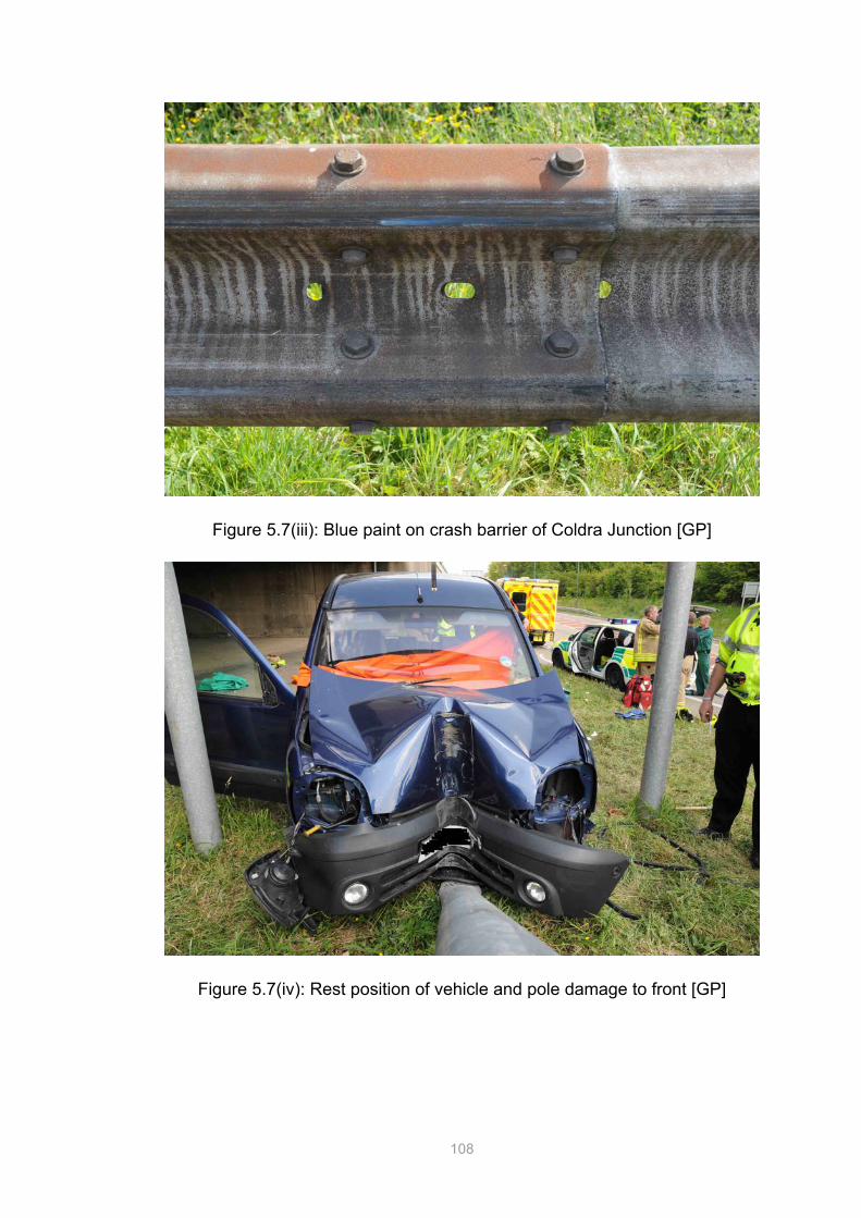
impact from the scene. On the nearside crash barrier was an impact mark
with scrapes and similar blue paint to that of the Renault. Approximately 90m
from this point, blue paint and scrape marks were seen on the junction wall at
a height of ½ metre. From this point, tyre tracks lead away from the wall
towards the carriageway and left the verge after a further 23.2 metres.
[GP]: The grass within the tyre mark was inspected and it was formed by
being simply laid flat. The grass indicated that the wheels were rolling and
not braking, as there were no plucked or torn grass stems within the mark.
The vehicle came to rest at the centre post of a roadsign located at the end
of the slip road. The post had been dislodged by the impact and was bent
over to an angle of approximately 30º to the ground.
Figure 5.7(ii): Exit Sliproad of Coldra Junction Crash [GP]
108
Figure 5.7(iii): Blue paint on crash barrier of Coldra Junction [GP]
Figure 5.7(iv): Rest position of vehicle and pole damage to front [GP]
109
Outcome [SJU]:
• Vehicle 1: Renault Kangoo, medium speed
• V = 40 mph, Deformation = 26cm
The RTA evidence [GP] reported that 3 passengers were in the vehicle, the
driver and passenger, whom were wearing seat belts, and a passenger in the
rear seat who was not. The first collision with the nearside crash barrier at
the top of the exit slip road for the junction could be described as a glancing
blow where the nearside of the car contacted the crash barrier, causing
relatively minor damage. This impact deflected the car away from the barrier
and across the sliproad.
[GP]: The car continued across the road and onto the offside verge and into
a concrete wall, again causing minor damage to the bodywork. After this
contact with the wall, the vehicle struck the centre post of a roadsign and
came to rest.
[SJU]: The vehicle in this case demonstrates how a lack of steering and
braking on a downhill section of road can cause the vehicle to ricochet off
roadside barriers and walls. The software concept of modelling roadside
features as solid objects with a large mass is representative in this respect.
110
RTA7 Slideshow
Figure 5.7 (v-xi): Coldra Junction Crash [SJU]
The vehicle exits the sliproad from the motorway, but for unknown reasons veers from the normal left-hand exit lane into the roadside barrier. Contact is made with the roadside barrier at a known point, measured by the RTA Investigator. This is modelled as 3 short sideswipe impacts. The vehicle then rebounds from the barrier to the right.
The vehicle now veers right across two lanes towards the concrete wall of the overhead motorway. Again, no evidence of braking or steering was recorded by the RTA. At contact with the wall the software reconstructs this collision as 3 short sideswipes. The vehicle then rebounds to the left again, heading towards the main junction roundabout. Before the vehicle can reach the roundabout, a frontal impact with a pole occurs, stopping the vehicle suddenly and dislodging the pole.
As part of the case file was CCTV footage taken from a motorway camera mounted high above the carriageway, two viewpoints from this camera position are given. On the left, the vehicle is shown heading towards the first impact with the side barrier. On the right, the subsequent rebound towards the junction wall is given.
111
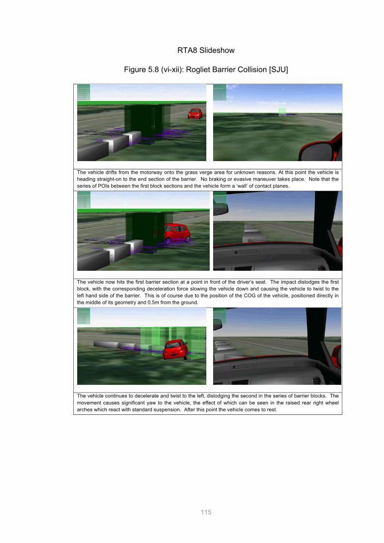
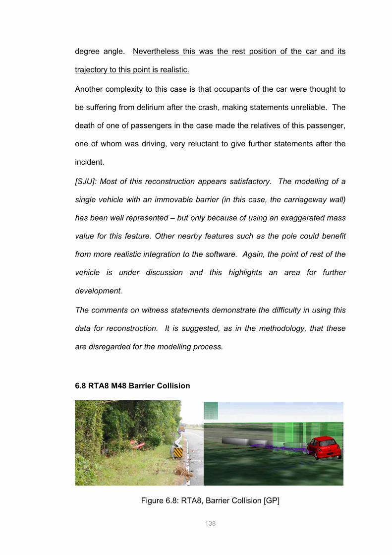
5.8 RTA8: M48 Rogliet, Head-on Collision with Emergency Barrier
Study: A case demonstrating the reconstruction of a small vehicle striking a
roadside barrier head-on. The complex barrier geometry has been
represented by a series of blocks with mass and friction to model
deceleration of the vehicle.
• 1 Vehicle impacted with object
• Motorway, Daytime, 2012
• No serious injuries, subsequent fatality following incident
• Scene attended by RTA Investigator
Scenario [GP]: A driver was travelling along the M48 motorway in clear light.
At some point the vehicle drifted to the left hand side of the carriageway, onto
the grass verge and impacted with the initial section of the roadside barrier
(yellow/black stripe). No obstacles or collisions with other vehicles were
noted or suspected. The barrier absorbed the momentum of the vehicle and
brought the car to rest in a clump of trees to the left of the verge.
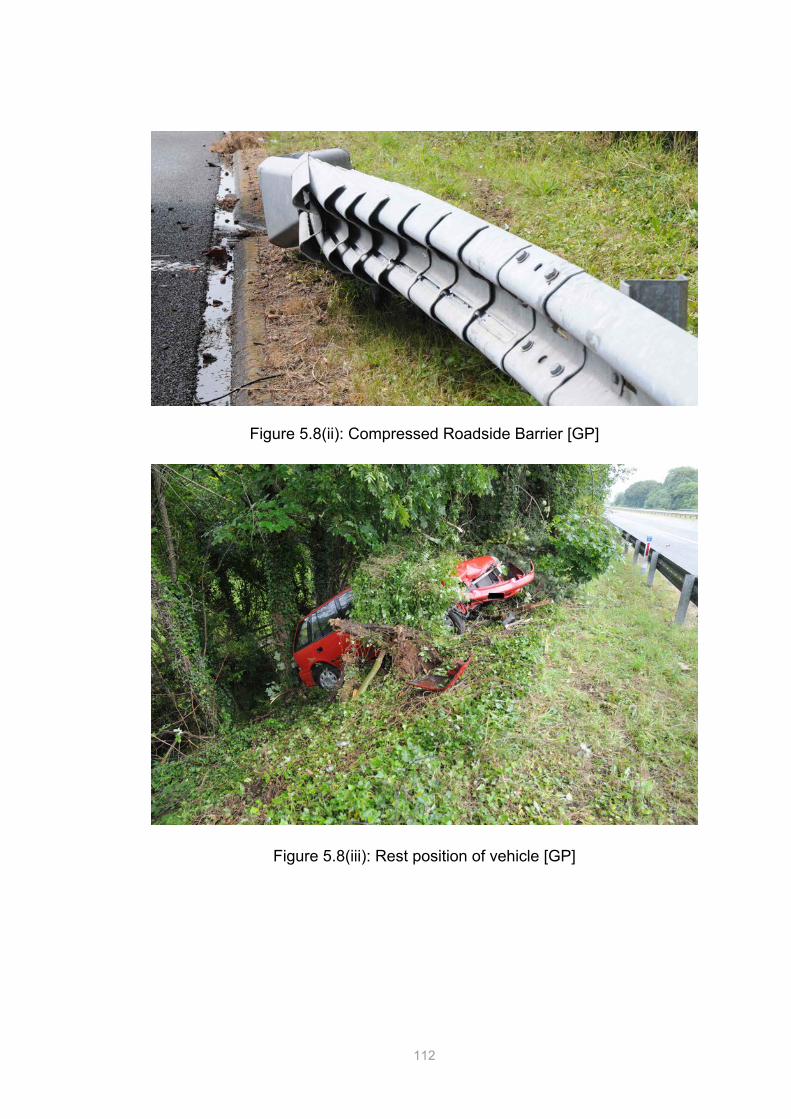
Figure 5.8(i): Rogliet Barrier Collision [GP]
112
Figure 5.8(ii): Compressed Roadside Barrier [GP]
Figure 5.8(iii): Rest position of vehicle [GP]
113
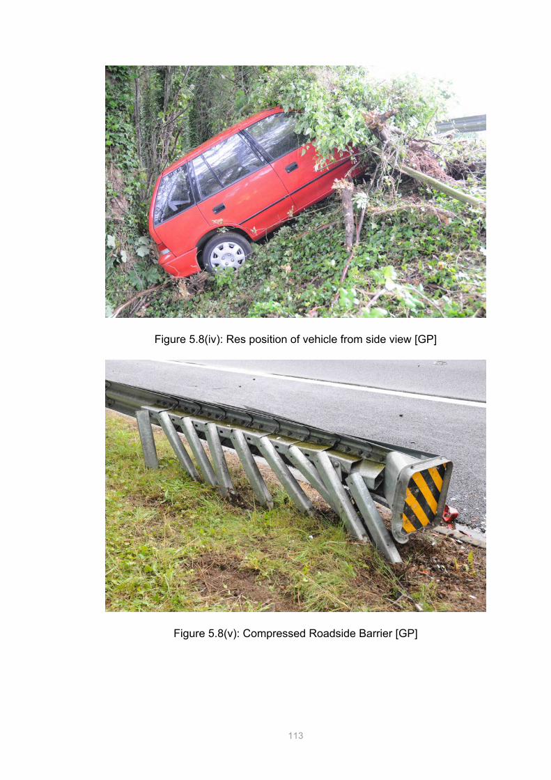
Figure 5.8(iv): Res position of vehicle from side view [GP]
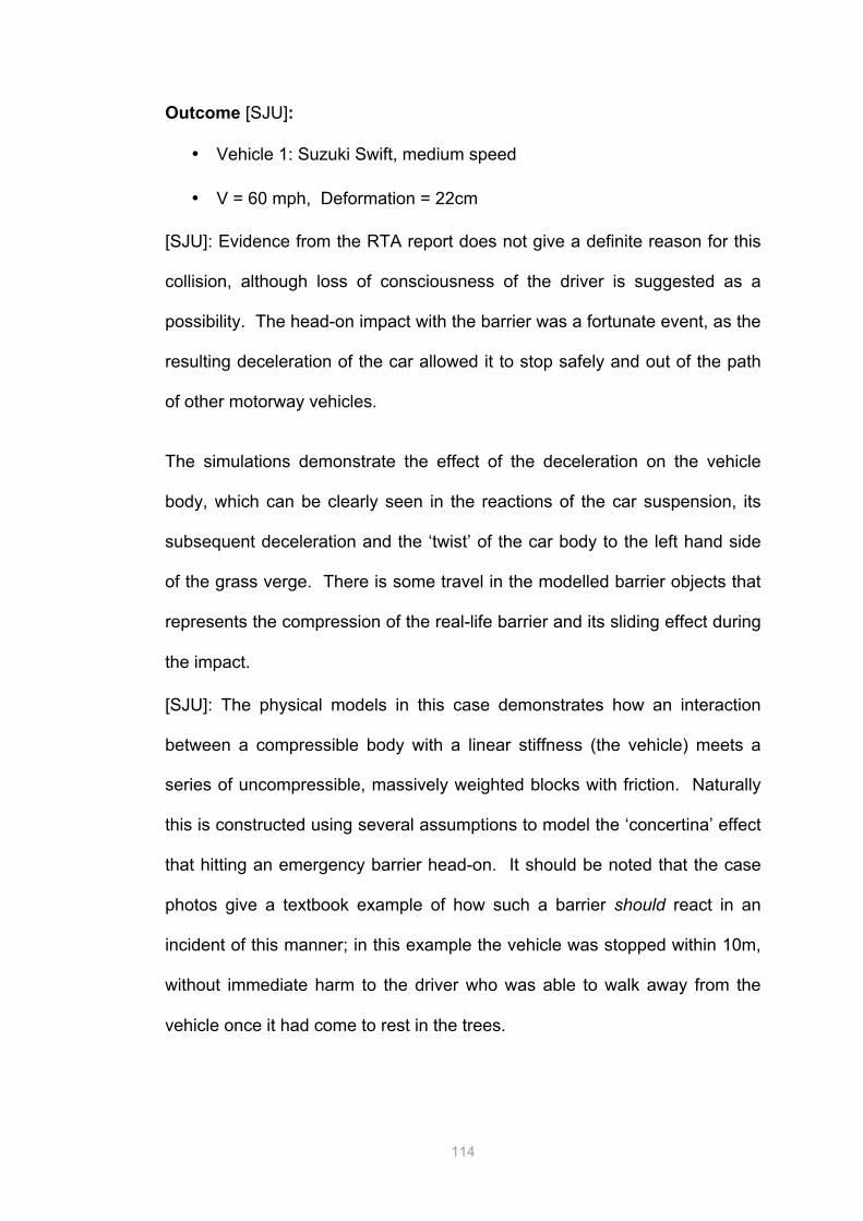
Figure 5.8(v): Compressed Roadside Barrier [GP]
114
Outcome [SJU]:
• Vehicle 1: Suzuki Swift, medium speed
• V = 60 mph, Deformation = 22cm
[SJU]: Evidence from the RTA report does not give a definite reason for this
collision, although loss of consciousness of the driver is suggested as a
possibility. The head-on impact with the barrier was a fortunate event, as the
resulting deceleration of the car allowed it to stop safely and out of the path
of other motorway vehicles.
The simulations demonstrate the effect of the deceleration on the vehicle
body, which can be clearly seen in the reactions of the car suspension, its
subsequent deceleration and the ‘twist’ of the car body to the left hand side
of the grass verge. There is some travel in the modelled barrier objects that
represents the compression of the real-life barrier and its sliding effect during
the impact.
[SJU]: The physical models in this case demonstrates how an interaction
between a compressible body with a linear stiffness (the vehicle) meets a
series of uncompressible, massively weighted blocks with friction. Naturally
this is constructed using several assumptions to model the ‘concertina’ effect
that hitting an emergency barrier head-on. It should be noted that the case
photos give a textbook example of how such a barrier should react in an
incident of this manner; in this example the vehicle was stopped within 10m,
without immediate harm to the driver who was able to walk away from the
The vehicle drifts from the motorway onto the grass verge area for unknown reasons. At this point the vehicle is heading straight-on to the end section of the barrier. No braking or evasive maneuver takes place. Note that the series of POIs between the first block sections and the vehicle form a ‘wall’ of contact planes.
The vehicle now hits the first barrier section at a point in front of the driver’s seat. The impact dislodges the first block, with the corresponding deceleration force slowing the vehicle down and causing the vehicle to twist to the left hand side of the barrier. This is of course due to the position of the COG of the vehicle, positioned directly in the middle of its geometry and 0.5m from the ground.
The vehicle continues to decelerate and twist to the left, dislodging the second in the series of barrier blocks. The movement causes significant yaw to the vehicle, the effect of which can be seen in the raised rear right wheel arches which react with standard suspension. After this point the vehicle comes to rest.
116
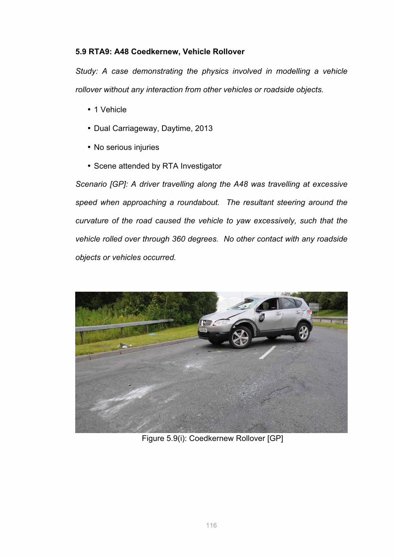
5.9 RTA9: A48 Coedkernew, Vehicle Rollover
Study: A case demonstrating the physics involved in modelling a vehicle
rollover without any interaction from other vehicles or roadside objects.
• 1 Vehicle
• Dual Carriageway, Daytime, 2013
• No serious injuries
• Scene attended by RTA Investigator
Scenario [GP]: A driver travelling along the A48 was travelling at excessive
speed when approaching a roundabout. The resultant steering around the
curvature of the road caused the vehicle to yaw excessively, such that the
vehicle rolled over through 360 degrees. No other contact with any roadside
objects or vehicles occurred.
Figure 5.9(i): Coedkernew Rollover [GP]
117
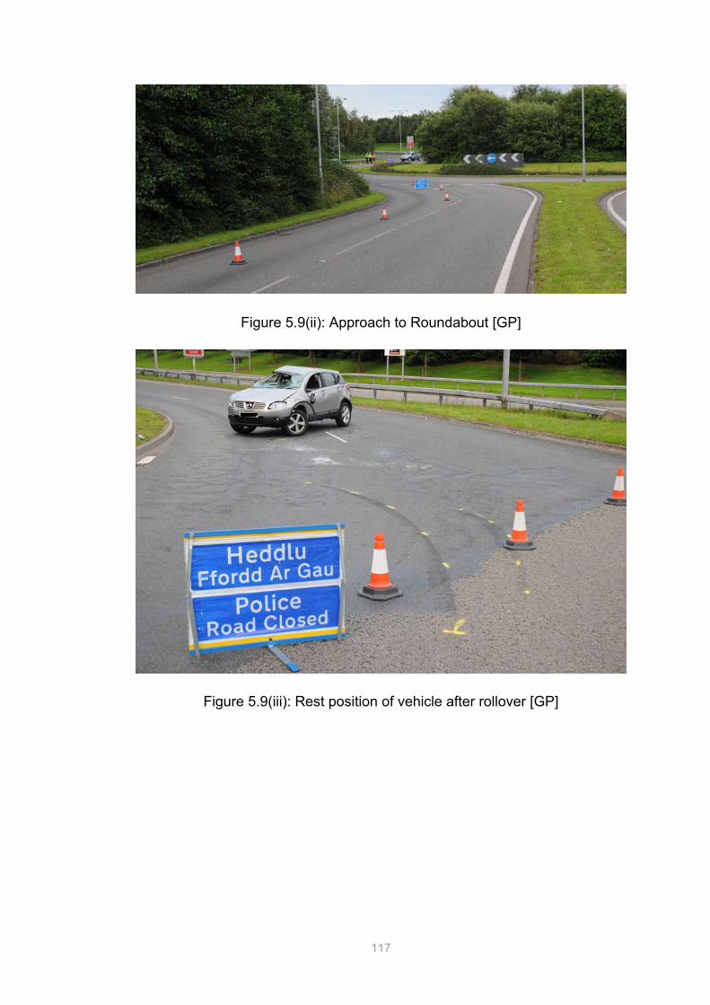
Figure 5.9(ii): Approach to Roundabout [GP]
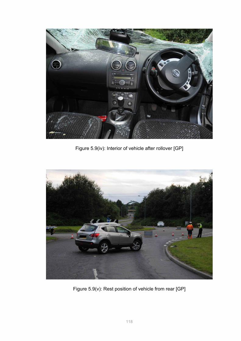
Figure 5.9(iii): Rest position of vehicle after rollover [GP]
118
Figure 5.9(iv): Interior of vehicle after rollover [GP]
Figure 5.9(v): Rest position of vehicle from rear [GP]
119
Outcome [GP]:
• Vehicle 1: Nissan Qashqai, Excessive speed
• V = 56 mph, Deformation = N/A
[GP]: The evidence showed that as the Nissan entered the left hand bend on
the entrance to the Roundabout, it was travelling at a speed of 56 mph,
losing control. The driver then attempted to steer the car leftwards to avoid
the roundabout, causing the vehicle to spin in a clockwise direction.
[GP]: The driver has again attempted to correct the ‘over steer’ when heading
towards the eastern exit onto the A48, causing the car to yaw rapidly and
spin in a anticlockwise direction. The resultant forces on the tyres were
sufficient to cause the alloy wheels to make contact with the road surface,
marking the road. Past this point the momentum and yaw of the car caused
it to overturn onto its roof, then coming to rest in the middle of the eastbound
lane.
The evidence shows that the distance from leaving the first skid mark to the
point where the car overturned was over 98 metres. A car travelling at 50
mph could stop in 26 metres, hence the speed of this vehicle was excessive.
[SJU]: This case demonstrates that the physical forces involved in a non-
contact incident can be accurately represented. Attributes such as COG and
suspension stiffness are vital in giving a meaningful interpretation of the
incident.
120
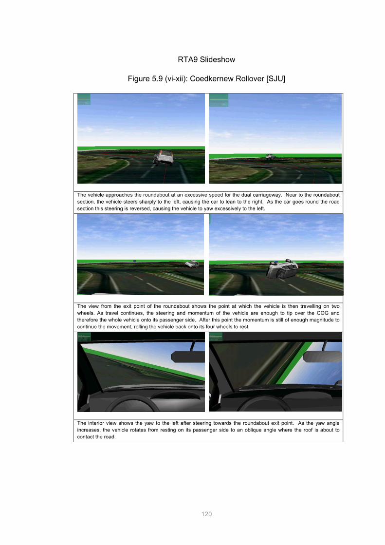
RTA9 Slideshow
Figure 5.9 (vi-xii): Coedkernew Rollover [SJU]
The vehicle approaches the roundabout at an excessive speed for the dual carriageway. Near to the roundabout section, the vehicle steers sharply to the left, causing the car to lean to the right. As the car goes round the road section this steering is reversed, causing the vehicle to yaw excessively to the left.
The view from the exit point of the roundabout shows the point at which the vehicle is then travelling on two wheels. As travel continues, the steering and momentum of the vehicle are enough to tip over the COG and therefore the whole vehicle onto its passenger side. After this point the momentum is still of enough magnitude to continue the movement, rolling the vehicle back onto its four wheels to rest.
The interior view shows the yaw to the left after steering towards the roundabout exit point. As the yaw angle increases, the vehicle rotates from resting on its passenger side to an oblique angle where the roof is about to contact the road.
121
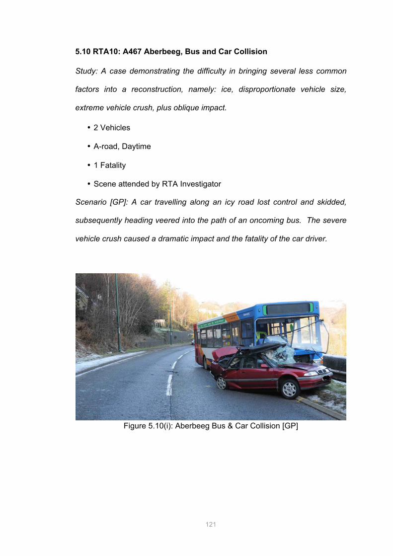
5.10 RTA10: A467 Aberbeeg, Bus and Car Collision
Study: A case demonstrating the difficulty in bringing several less common
factors into a reconstruction, namely: ice, disproportionate vehicle size,
extreme vehicle crush, plus oblique impact.
• 2 Vehicles
• A-road, Daytime
• 1 Fatality
• Scene attended by RTA Investigator
Scenario [GP]: A car travelling along an icy road lost control and skidded,
subsequently heading veered into the path of an oncoming bus. The severe
vehicle crush caused a dramatic impact and the fatality of the car driver.
Figure 5.10(i): Aberbeeg Bus & Car Collision [GP]
122
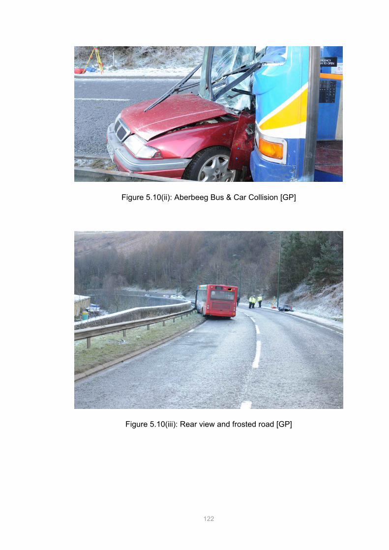
Figure 5.10(ii): Aberbeeg Bus & Car Collision [GP]
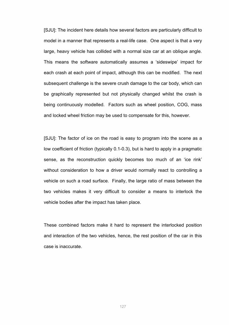
Figure 5.10(iii): Rear view and frosted road [GP]
123
Figure 5.10(iv): Severe vehicle crush of Bus & Car bodies [GP]
Figure 5.10(v): Side view, severe vehicle crush of Bus & Car bodies [GP]
124
Outcome [SJU]:
• Vehicle 1: Rover 216
• V = 35 mph, Deformation = 34cm
• Vehicle 2: Dennis Single-Level Passenger Bus
• V = 39 mph, Deformation = 11cm
[SJU]: The environment surrounding this incident was highly influential in the
action of the drivers and the trajectory of the vehicles involved, as it was a
very cold and dry day. [GP] The road temperature was measured at between
-7°C and -9°C, and black ice was present on the road surface.
[GP]: The driver of the Rover was travelling on the A467 in a northerly
direction, and appeared to be wearing their seat belt at the time of the
collision. On a right hand bend it lost control and started to spin in a
clockwise direction, crossing the centre white line and rotating to a broad
angle to oncoming traffic.
[GP]: The Bus operated by Stagecoach was travelling in the opposite
direction. The car had skidded for 33 metres before impacting into the front
offside corner of the bus. After this impact, the vehicle bodies of the bus and
Rover were interlocked and took 21 metres to come to rest near the left-hand
side of the road.
125
RTA10 Slideshow I
Figure 5.10(vi-xii): Aberbeeg Bus & Car Collision [SJU]
The car is travelling round the curve of the road and begins to lose control, with right lock being applied to the steering. At this point all four wheels have made contact with the low-friction portion of the road designated as ice. This portion can be seen as a black-lined polygon. From the opposing point of view of the bus driver, the car is now becoming visible.
The momentum of the car continues as further right wheel lock and full braking is applied. The car is now out of control and continues to skid across the ice over to the right-hand side of the road. This point now represents the image of the bus CCTV footage included in the appendix. The exact reaction point of the bus driver is not known but this position would be a reasonable estimate.
The car continues along its trajectory, rotating clockwise as it does. Imminently before the collision the car is about to contact the opposing grass verge. Note that the contact plane at the POI is almost parallel to the car body.
126
RTA10 Slideshow II
Figure 5.10 (xiii-ix): Aberbeeg Bus & Car Collision [SJU]
At the POI, the bus impacts the car at the area of the passenger side door, with an angle of impact approximately 30 degrees to the longitudinal axis of the car body. Full steering lock and braking is still applied to the car at the point. The bus driver would have a view above the impact area.
Immediately after the impact, there are no modelled forces to represent the interlocking of the vehicle bodies. The rotation of the car body continues against the bus, with the low friction of the ice underneath encouraging further skidding. This modelled situation allows the car body to separate from the bus. The bus then drifts to the left, hitting the grass verge.
The car continues to skid and rotate, heading away from the bus. The minimal friction on the ice allows it to stop on the right hand side of the road. The bus is now in contact with the grass verge (designated as a high-friction area) and comes to a stop.
127
[SJU]: The incident here details how several factors are particularly difficult to
model in a manner that represents a real-life case. One aspect is that a very
large, heavy vehicle has collided with a normal size car at an oblique angle.
This means the software automatically assumes a ‘sideswipe’ impact for
each crash at each point of impact, although this can be modified. The next
subsequent challenge is the severe crush damage to the car body, which can
be graphically represented but not physically changed whilst the crash is
being continuously modelled. Factors such as wheel position, COG, mass
and locked wheel friction may be used to compensate for this, however.
[SJU]: The factor of ice on the road is easy to program into the scene as a
low coefficient of friction (typically 0.1-0.3), but is hard to apply in a pragmatic
sense, as the reconstruction quickly becomes too much of an ‘ice rink’
without consideration to how a driver would normally react to controlling a
vehicle on such a road surface. Finally, the large ratio of mass between the
two vehicles makes it very difficult to consider a means to interlock the
vehicle bodies after the impact has taken place.
These combined factors make it hard to represent the interlocked position
and interaction of the two vehicles, hence, the rest position of the car in this
case is inaccurate.
128
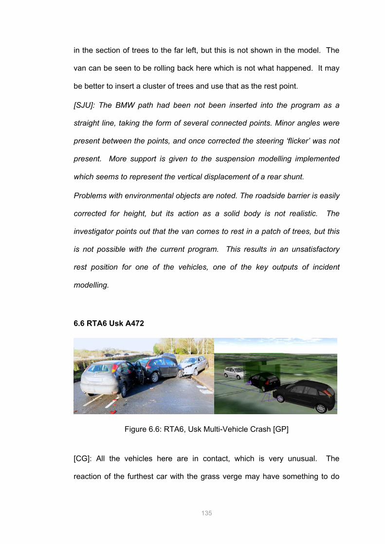
6. Discussion of Results & Professional Feedback
The caseload of simulated RTA Incidents were then presented back to PC
Goddard at Gwent Police. The officer was shown the scenes in the form of
several 2D and 3D reconstructions, and asked to give direct and critical
feedback regarding the suitability and accuracy of the software for collision
modelling. The table below shows the RTA caseload given and areas which
were said to require modification in order to be accurate and meaningful to
the incident.
RTA Location
Modification was Requested to the Following Parameters:
Vehicle & Settings Speed Layout &
Environment Collision/
POI Friction,
Restitution
1 Example No No No No No
2 Plymouth No No No No No
3 Warnham No Yes No No No
4 Danbury No No No Yes No
5 Usk A449 Yes No Yes No No
6 Usk A472 Yes No No Yes No
7 Coldra M4 No No Yes No No
8 M48 Barrier No Yes Yes No No
9 Coedkernew Yes No No No Yes
10 Aberbeeg Yes No Yes No Yes
Table 6.1: Modifications requested to reconstructions in caseload.
The comments of the officer [CG] are given in an edited form that extracts
most of the conversational element of the feedback. The most pertinent
points to the reconstructions have been underlined; some reflection [SJU] is
given to each of these points, as well as other commentary from PC
Goddard.
129
6.1 RTA1 Example
Figure 6.1: RTA1, Example
[CG]: This is a very simple example so it is difficult to comment. It isn’t a real
case so it simply appears that the impact is just that. There is movement in
the car suspension which is appropriate, but there is not really more to add.
[SJU]: This is indeed an ‘example case’. The note of vehicle suspension is
worth commentary as this is one of the advantages of the PC-Crash
software, given that suspension is modelled realistically and may be adjusted
widely.
6.2 RTA2 Plymouth
Figure 6.2: RTA2, Plymouth Low-Velocity Collision
[CG]: It would be beneficial to know if there was any displacement of the red
vehicle (the stationary car on the left). A lot of the impact at low speed will be
absorbed by the suspension alone. It appears that the red car has not moved
130
at all with a very small rebound from the blue car. This would be expected in
a normal low-speed collision.
[SJU]: There was no information on post-impact displacment available from
the public domain source. Commentary above demonstrates that the
potential investigating low-speed crashes is very limited, due to the small
amount of damage to vehicle bodies, lack of tyres marks, debris, and so
forth. This type of incident still remains less popular among Forensic
Investigators, although dashcams have become widespread in use as a
means of recording such impacts.
6.3 RTA3 Warnham
Figure 6.3: RTA3, Warnham High-Velocity Collision
[CG]: A staged incident set up for controlled crash research resembled this
case very closely. The staged incident here used a Peugeot 206 with an
Astra in a perpendicular T-bone impact. In this incident, the force of the
impact tilted the impacted car significantly. Looking at the Golf (in Figure
5.3ii) the damage is appears comparable, which suggests the speeds are
relative; 50mph in the setup test and 60mph in the RTA3 case. The
suspension of the impacted car would have moved sharply on impact,
absorbing a little of the kinetic energy.
131
Here the simulated case does not appear very different from the real vehicle-
to-vehicle interactions.
[SJU]: The integration of vehicle suspension features to the program is given
some more validation here. More interestingly, this case outlines a general
type of crash (the t-bone, common at junctions) that appears to have been
modelled well with regard to simulating this scenario accurately. There is an
advantage to this case in that both vehicles are approximately the same
mass and dimensions. The accuracy of the modelling could well diminish if
this was not the case (requires further research).
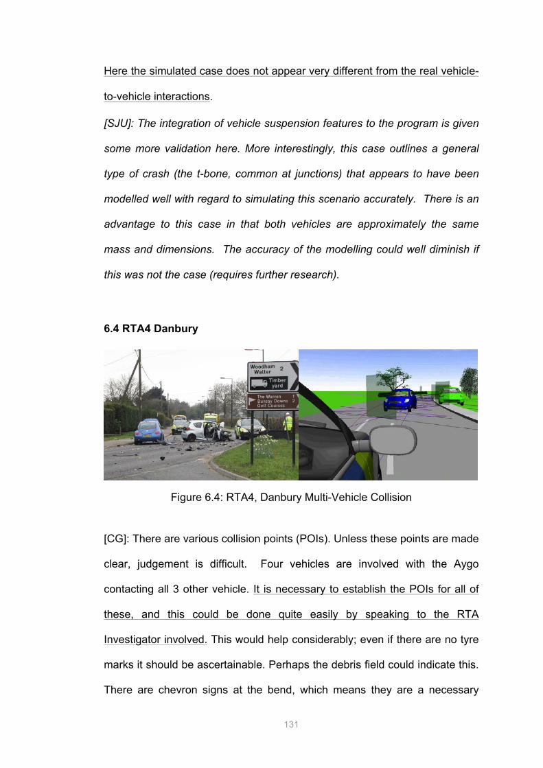
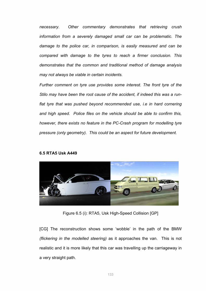
6.4 RTA4 Danbury
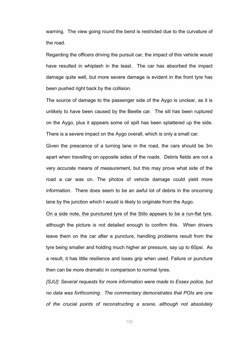
Figure 6.4: RTA4, Danbury Multi-Vehicle Collision
[CG]: There are various collision points (POIs). Unless these points are made
clear, judgement is difficult. Four vehicles are involved with the Aygo
contacting all 3 other vehicle. It is necessary to establish the POIs for all of
these, and this could be done quite easily by speaking to the RTA
Investigator involved. This would help considerably; even if there are no tyre
marks it should be ascertainable. Perhaps the debris field could indicate this.
There are chevron signs at the bend, which means they are a necessary
132
warning. The view going round the bend is restricted due to the curvature of
the road.
Regarding the officers driving the pursuit car, the impact of this vehicle would
have resulted in whiplash in the least. The car has absorbed the impact
damage quite well, but more severe damage is evident in the front tyre has
been pushed right back by the collision.
The source of damage to the passenger side of the Aygo is unclear, as it is
unlikely to have been caused by the Beetle car. The sill has been ruptured
on the Aygo, plus it appears some oil spill has been splattered up the side.
There is a severe impact on the Aygo overall, which is only a small car.
Given the prescence of a turning lane in the road, the cars should be 3m
apart when travelling on opposite sides of the roads. Debris fields are not a
very accurate means of measurement, but this may prove what side of the
road a car was on. The photos of vehicle damage could yield more
information. There does seem to be an awful lot of debris in the oncoming
lane by the junction which I would is likely to originate from the Aygo.
On a side note, the punctured tyre of the Stilo appears to be a run-flat tyre,
although the picture is not detailed enough to confirm this. When drivers
leave them on the car after a puncture, handling problems result from the
tyre being smaller and holding much higher air pressure, say up to 60psi. As
a result, it has little resilience and loses grip when used. Failure or puncture
then can be more dramatic in comparison to normal tyres.
[SJU]: Several requests for more information were made to Essex police, but
no data was forthcoming. The commentary demonstrates that POIs are one
of the crucial points of reconstructing a scene, although not absolutely
133
necessary. Other commentary demonstrates that retrieving crush
information from a severely damaged small car can be problematic. The
damage to the police car, in comparison, is easily measured and can be
compared with damage to the tyres to reach a firmer conclusion. This
demonstrates that the common and traditional method of damage analysis
may not always be viable in certain incidents.
Further comment on tyre use provides some interest. The front tyre of the
Stilo may have been the root cause of the accident, if indeed this was a run-
flat tyre that was pushed beyond recommended use, i.e in hard cornering
and high speed. Police files on the vehicle should be able to confirm this,
however, there exists no feature in the PC-Crash program for modelling tyre
pressure (only geometry). This could be an aspect for future development.
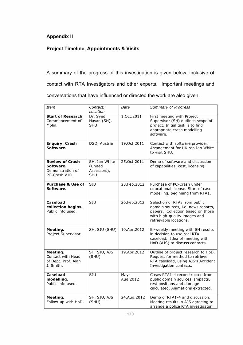
A summary of the progress of this investigation is given below, inclusive of
contact with RTA Investigators and other experts. Important meetings and
conversations that have influenced or directed the work are also given.
Item Contact, Location
Date Summary of Progress
Start of Research. Commencement of Mphil.
Dr. Syed Hasan (SH), SHU
1.Oct.2011 First meeting with Project Supervisor (SH) outlines scope of project. Initial task is to find appropriate crash modelling software.
Enquiry: Crash Software.
DSD, Austria 19.Oct.2011 Contact with software provider. Arrangement for UK rep Ian White to visit SHU.
Review of Crash Software. Demonstration of PC-Crash v10.
SH, Ian White (United Assessors), SHU
25.Oct.2011 Demo of software and discussion of capabilities, cost, licensing.
Purchase & Use of Software.
SJU 23.Feb.2012 Purchase of PC-Crash under educational license. Start of case modelling, beginning from RTA1.
Caseload collection begins. Public info used.
SJU 26.Feb.2012 Selection of RTAs from public domain sources, i.e. news reports, papers. Collection based on those with high-quality images and retrievable locations.
Meeting. Project Supervisor.
SH, SJU (SHU) 10.Apr.2012 Bi-weekly meeting with SH results in decision to use real RTA caseload. Idea of meeting with HoD (AJS) to discuss contacts.
Meeting. Contact with Head of Dept. Prof. Alan J. Smith.
SH, SJU, AJS (SHU)
19.Apr.2012 Outline of project research to HoD. Request for method to retrieve RTA caseload, using AJS’s Accident Investigation contacts.
Caseload modelling. Public info used.
SJU May-Aug.2012
Cases RTA1-4 reconstructed from public domain sources. Impacts, rest positions and damage calculated. Animations extracted.
Meeting. Follow-up with HoD.
SH, SJU, AJS (SHU)
24.Aug.2012 Demo of RTA1-4 and discussion. Meeting results in AJS agreeing to arrange a police RTA investigator
171
as main project contact.
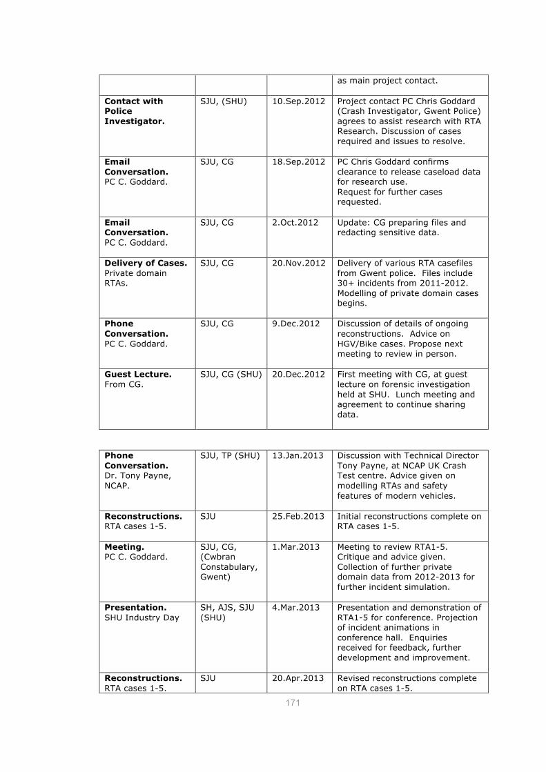
Contact with Police Investigator.
SJU, (SHU) 10.Sep.2012 Project contact PC Chris Goddard (Crash Investigator, Gwent Police) agrees to assist research with RTA Research. Discussion of cases required and issues to resolve.
Email Conversation. PC C. Goddard.
SJU, CG 18.Sep.2012 PC Chris Goddard confirms clearance to release caseload data for research use. Request for further cases requested.
SJU, CG 20.Nov.2012 Delivery of various RTA casefiles from Gwent police. Files include 30+ incidents from 2011-2012. Modelling of private domain cases begins.
Phone Conversation. PC C. Goddard.
SJU, CG 9.Dec.2012 Discussion of details of ongoing reconstructions. Advice on HGV/Bike cases. Propose next meeting to review in person.
Guest Lecture. From CG.
SJU, CG (SHU) 20.Dec.2012 First meeting with CG, at guest lecture on forensic investigation held at SHU. Lunch meeting and agreement to continue sharing data.
Phone Conversation. Dr. Tony Payne, NCAP.
SJU, TP (SHU) 13.Jan.2013 Discussion with Technical Director Tony Payne, at NCAP UK Crash Test centre. Advice given on modelling RTAs and safety features of modern vehicles.
Reconstructions. RTA cases 1-5.
SJU 25.Feb.2013 Initial reconstructions complete on RTA cases 1-5.
Meeting. PC C. Goddard.
SJU, CG, (Cwbran Constabulary, Gwent)
1.Mar.2013 Meeting to review RTA1-5. Critique and advice given. Collection of further private domain data from 2012-2013 for further incident simulation.
Presentation. SHU Industry Day
SH, AJS, SJU (SHU)
4.Mar.2013 Presentation and demonstration of RTA1-5 for conference. Projection of incident animations in conference hall. Enquiries received for feedback, further development and improvement.
Reconstructions. RTA cases 1-5.
SJU 20.Apr.2013 Revised reconstructions complete on RTA cases 1-5.
172
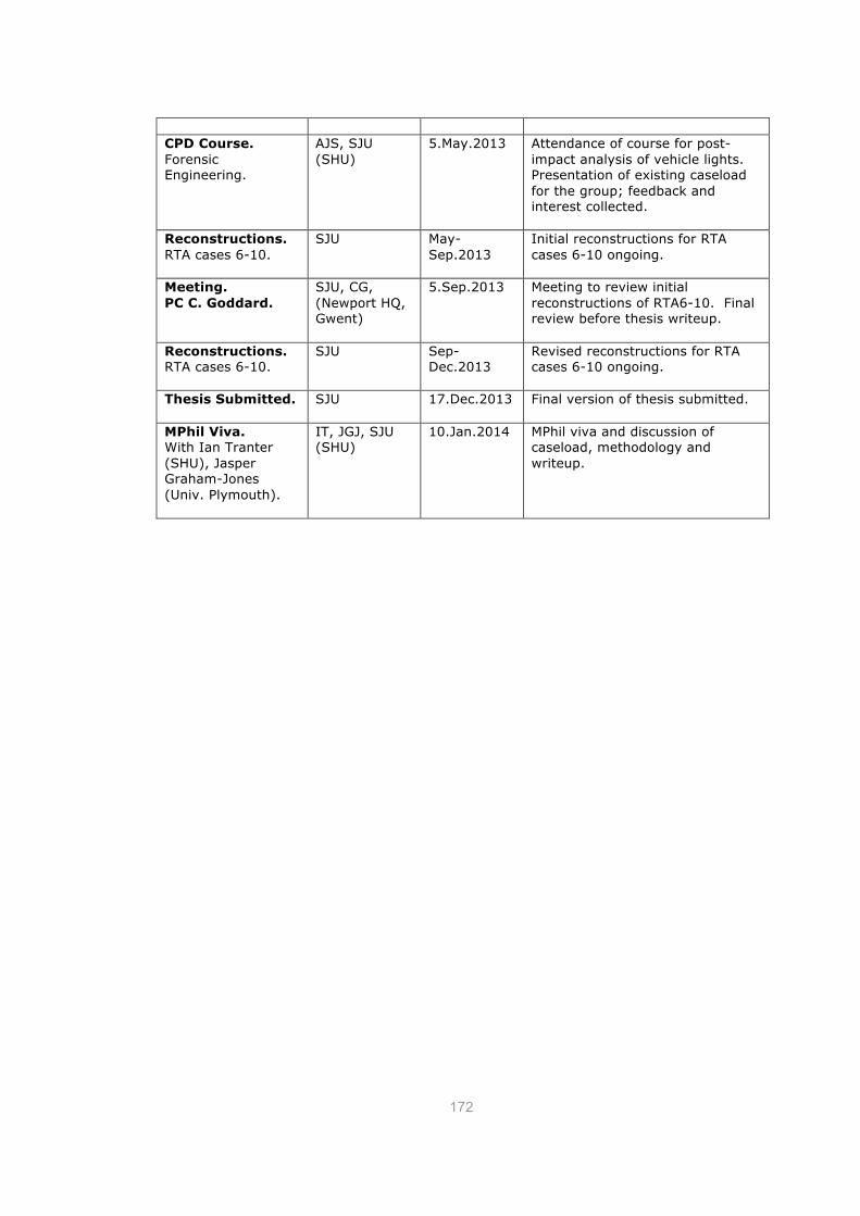
CPD Course. Forensic Engineering.
AJS, SJU (SHU)
5.May.2013 Attendance of course for post-impact analysis of vehicle lights. Presentation of existing caseload for the group; feedback and interest collected.
Reconstructions. RTA cases 6-10.
SJU May-Sep.2013
Initial reconstructions for RTA cases 6-10 ongoing.
Meeting. PC C. Goddard.
SJU, CG, (Newport HQ, Gwent)
5.Sep.2013 Meeting to review initial reconstructions of RTA6-10. Final review before thesis writeup.
Reconstructions. RTA cases 6-10.
SJU Sep-Dec.2013
Revised reconstructions for RTA cases 6-10 ongoing.
Thesis Submitted.
SJU 17.Dec.2013 Final version of thesis submitted.
MPhil Viva. With Ian Tranter (SHU), Jasper Graham-Jones (Univ. Plymouth).
IT, JGJ, SJU (SHU)
10.Jan.2014 MPhil viva and discussion of caseload, methodology and writeup.
MERI Health and Safety Plan - Desk based students only 2008 page
Project Safety Plan 2011/2 Date: 20.10.2012 (project start date or first planning meeting with DoS) DESK BASED STUDENTS only
STUDENT NAME URQUHART, Simon DoS
NAME Syed T. Hasan
Project Title Vehicle Collision Modelling
Short Summary of project activities
Computer modelling of road traffic accidents (project involves desk work only).
Safety training for first month including Induction
Date:
DoS Signature:
Student Signature:
Attended University Induction Session 21.11.2011
Attended MERI Induction Programme 02.11.2011 Attended Fire Awareness Training session 05.12.2011
You must know : Where your Fire Evacuation Assembly Point is: you can find this on the blue wall signs Who the First-Aiders in your area are: you can find this on the green wall signs In case of an emergency you must ring X888 and explain the problem and give your location