DEMOGRAPHY© Volume 11, Number 4 November 1974

THE FORMAL DYNAMICS OF CONTROLLED POPULATIONSAND THE ECHO, THE BOOM AND THE BUST

Ronald LeeDepartment of Economics and Population Studies Center, University of Michigan,1225 S. University Ave., Ann Arbor, Michigan 48104

Abstract-This paper analyzes the pattern of fluctuations of births in an age­structured population whose growth is subject to environmental or eco­nomic constraint. It synthesizes the traditional demographic analysis ofage-structured renewal with constant vital rates and the economic analysiswhich treats population change endogenously. When cohort fertility de­pends on relative cohort size, or when period fertility depends on laborforce size, fluctuations of forty or more years replace the traditional "echo"or generation-length cycle. Twentieth-century U. S. fertility change agreeswell with the theory, as the "Easterlin Hypothesis" suggests; but the periodmodel fits better than the cohort model.

1. INTRODUCTION the reversal of the echo effect, are re-All populations are subject to environ- garded from this point of view.

mental constraint in one form or another, Numerous models express an assumedand because their potential growth is so long-run tendency of population to equil­rapid, they are typically found near equi- ibrate with productive capacity. Manylibrium, where the constraints operate of these derive from the populationeffectively through checks on population theory of classical economics and aregrowth and size. So Malthus argued; and exemplified by the work of Leibensteinthis paper explores the implications of his (1963), Solow (1956) and Lee (1970,view for the analysis of population dy- 1973, 1974b). Others are extensions tonamics. human populations of models devel-

However, despite an extensive litera- oped for animal ecology, as in the workture on the economics of fertility and the of Pearl (1924), Birdsell (1957), Sauvymacroeconomic effects of population (1969) and Wrigley (1969). There is re­growth, there is little direct evidence that lated work by animal population ecol­population is an endogenous component ogists with which this author can claimin an equilibrating system. The approach little familiarity. Most of these modelsof this paper is indirect: we assume that are static or, if dynamic, ignore the agepopulation is near equilibrium and de- structure of the population and the vari­rive the consequences for the dynamics ous lags which occur in the adjustmentof population renewal. Comparison of process. But oscillations are characteris­actual population dynamics to the be- tic of controlled systems, since sensitivehavior implied by the model may then regulation, operating with a response lag,shed light on the questions of whether a can lead to overshooting of equilibriumcontrol system exists, and if so, how it and what we will call "control cycles."operates. In particular, the U. S. baby Thus, while abstraction from lags andboom and baby bust, characterized by age structure may be appropriate for the

563

564 DEMOGRAPHY, volume 11, number 4, November 1974

long run, for many applications we willwant to know more about the conver­gence path of population, about the sta­bility of equilibrium, and about the cyclictendencies of the system.

There is also an extensive body of lit­erature analyzing the dynamic behaviorof age-structured populations as theyproceed from an initially disturbed stateto steady exponential growth, under theassumption of constant vital rates. Thiswork derives from the models and analy­sis of Lotka, the pioneer mathematicaldemographer, and includes contributionsby Bernardelli (1941), Keyfitz (1965),Coale (1972) and LeBras (1969). Thiswork establishes a tendency for humanpopulations to move in cycles of onegeneration, or twenty-five to thirty­three years; we will call these "genera­tional cycles" or "echos." However, allthe models either assume that vital ratesare constant or that they vary indepen­dently of the size and structure of thepopulation; they thus abstract from theexistence of environmental constraints.

There has not yet been a general anal­ysis of population dynamics which incor­porates both the operation of constraintsand the age structure of the populationand thus relates the control cycle andgenerational cycle (although Keyfitz,1972, touches on closely related matters).However, there is a long tradition ofinteresting speculations regarding the dy­namic behavior arising from the inter­actions of the two. Malthus (1970) con­fidently asserted that population andwelfare perpetually oscillate about theirequilibria, due to the lag of labor supplybehind demand and the consequent over­reaction of net reproduction and capitalformation to prevailing conditions oflabor. Alfred Marshall expressed similarviews (Liu, 1971), and Yule (1906)argued for a periodicity of fifty to onehundred years.

More recently, it has been suggestedthat the time series of fertility in theUnited States might be due to a strong

negative reaction of fertility to cohortsize or potential labor force size; alongthese lines we have the contributions ofGrauman (1960), Easterlin (1962, 1968),Coale (1963), Ryder (1971), Lee (1970)and Keyfitz (1972). Easterlin, withwhose name this hypothesis is associated,has made the most careful empiricalstudies and, together with Condran(1974), has recently extended the analy­sis to several other industrial countries.

These studies suggest that an econom­ically endogenous population with agestructure might exhibit long control cy­cles in place of the classic echo effect. Ifso, the empirical analysis of populationfluctuations could provide evidence con­cerning the presence and nature of auto­regulatory mechanisms governing popu­lation growth.

Regular fluctuations in human popula­tions have long been observed. Someoscillations, with periods up to fifteenyears, are obviously imposed on demo­graphic series by the periodicity of cli­mate, epidemic, harvest, and the intrinsicdynamics of capitalist economies; others,like the twenty-year Kuznets cycle, mayreflect economic-demographic interac­tions (Easterlin, 1968). But these cyclesare superimposed on longer fluctuationsof less certain origin. The most widelyrecognized of these is a thirty-year cyclewhich is noticeable in the graphs of bap­tisms from many preindustrial parishes(see, e.g., Goubert, 1965). This could bean empirical manifestation of the "gen­erational" cycle, but we cannot reallytell without analyzing it in conjunctionwith stochastic models of the sort to bedeveloped in this paper.

Some observers also see evidence oflonger cycles in human populations, oflength closer to two generations, or fortyto sixty years. Thus the fifty-year Kon­dratieff cycle runs through the dem­ographic variables of nineteenth-centuryEurope and could possibly originate ina demographic control cycle. Similarly,there is a forty-year "cycle" in the fer-

Dynamics of Controlled Populations

tility of the United States in the twen­tieth century; it declines to a troughin the mid-thirties, rises to the "babyboom" peak in the late fifties, and de­clines in the "baby bust" thereafter. Thishas sometimes been interpreted as a con­trol cycle.

This paper develops a formal modelof renewal in an age-structured popula­tion subject to environmental constraint.We analyze the dynamics of the model ina way compatible with empirical estima­tion and testing. We conclude with anempirical application to U. S. fertility,1917 to 1972.

2. CONTROLLED POPULATION WITHOUT

AGE STRUCTURE

By a "controlled" population, we meanone which is endogenous to a systemwhich tends toward equilibrium. This re­quires that population growth respondpositively to variation in material wel­fare, while material welfare should inturn be depressed by population growth.For some level of material welfare, popu­lation will remain stationary and thesystem will be in equilibrium. The equi­librium levels of the system, and thespeed with which it converges, depend onsocial and economic institutions, tech­nology, and resources.

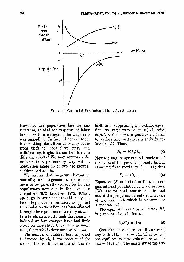
The basic system for a populationwithout age structure is illustrated inFigure 1. Aggregate fertility, measuredby the crude birth rate, b, is positivelyrelated to material welfare, w (whichcould be real wages, per capita income,average space, or any other appropriateconcept), with the form and level of therelation determined institutionally. (Fora discussion of relevant empirical work,see Simon, 1974.) This is represented bythe curve b(w). Mortality, measured bythe crude death rate, d, is negativelyrelated to w, as shown by the curve d(w) .At some level of welfare, b (w) andd (w) are equal, and the population istherefore stationary. This defines the

565

equilibrium welfare, WE, as noted on thediagram.

Welfare, w, is in turn negatively re­lated to population size, P, by a functionreflecting resources, reproducible capital,technology and social organization. Thebottom half of the diagram shows thisrelation, w(P), in inverted form. Finally,the relation w(P), together with WE, de­termines the equilibrium population size,P", as shown.

Every population size has a specificwage and a specific rate of populationgrowth, b (w) - d (w), associated withit. Inspection of Figure 1 shows that,when population is above equilibrium,mortality exceeds fertility and the pop­ulation declines; when population is be­low equilibrium, the opposite occurs.Thus, the equilibrium is stable.

We can be more explicit about thedynamics of the population when par­ticular equations for i. d and wareknown. For example, suppose that theseequations are all linear. Then the dif­ferential equation relating populationgrowth rates (PIP) to population sizewill also be linear:

PIP = a - cP (1)

for appropriate a and c. The solution tothis equation is the well-known logisticcurve, applied to human populations byPearl (1924) and many others. It has theform

P(t) = kl(l + e-a t) , (2)

where k = ale is the equilibrium popu­lation size.

For further development of this modeland for its estimation, testing and simu­lation based on historical data, see Lee(1970, 1973, 1974b).

3. CONTROLLED POPULATIONS WITH

Two AGE GROUPS

The model outlined in the last partconverged smoothly and steadily towardequilibrium following a disturbance.

566 DEMOGRAPHY, volume 11, number 4, November 1974

welfare

b(wl

l--__+--;:;- w

bd

io

t

pE\----f

PopulationP

Birthand

dC!othrates

FIGURE I.-Controlled Population without Age Structure

Consider once more the linear case,say with b (L t ) = a - cl.; Then by (5)the equilibrium birth cohort size will be(as - 1)/ (cs2 ) • The elasticity of the fer-

B l = b(LI)LI. (3)

Now the mature age group is made up ofsurvivors of the previous period's births,assuming fixed mortality (1 - s); thus

birth rate. Suppressing the welfare equa­tion, we may write b = b (L t ) , withdb/dL < 0 (since b is positively relatedto welfare and welfare is negatively re­lated to L). Thus,

(5)

(4)

Equations (3) and (4) describe the inter­generational population renewal process.(We assume that transition into andout of the groups occurs only at intervalsof one time unit, which is measured asa generation.)

The equilibrium number of births, BE,is given by the solution to

However, the population had no agestructure, so that the response of laborforce size to a change in the wage ratewas immediate. In fact, of course, thereis something like fifteen or twenty yearsfrom birth to labor force entry andchildbearing. Might this not lead to quitedifferent results? We may approach theproblem in a preliminary way with apopulation made up of two age groups:children and adults.

We assume that long-run changes inmortality are exogenous, which we be­lieve to be generally correct for humanpopulations now and in the past (seeChambers, 1972; Lee, 1970, 1973, 1974b),although in some contexts this may notbe so. Population adjustment, as opposedto population variation, has been effectedthrough the regulation of fertility at wel­fare levels sufficiently high that density­induced welfare changes have had littleeffect on mortality. Under this assump­tion, the model is developed as follows.

The number of children born in periodt, denoted by B t , is the product of thesize of the adult age group L, and its

Dynamics of Controlled Populations

tility function with respect to L is(1 - as). The difference equation will be

B, = (as)B I - 1 - (cl)Bl-1 2• (6)

Now this difference equation is veryclosely related to the logistic differentialequation, since with a little manipulationit can be represented in the form

tiBI/BI = e - fBI, (7)

with e = as - 1, and f = cs,". This ishardly surprising; the question is: Willthe solution also closely resemble thelogistic curve? This can be explored mostsimply with a diagram.

Let us represent the number of personsin the adult age group, L, on the hori­zontal axis and the number of births onthe vertical axis. Equations (3) and (4)may then be plotted as in Figure 2A.

From a point on the L axis we movevertically to find the number of birthson the B curve. We then advance a timeperiod (one generation or about thirtyyears) by moving horizontally to thenumber of adult survivors on the Lcurve. The process may now be repeated,leading to a steady convergence towardequilibrium from above or below theequilibrium point, indicated by the inter­section of the two curves. Recalling thateach horizontal move represents a gen­eration of time, we can plot the conver­gence of numbers of children or adults asin Figure 2B. The path closely resemblesa logistic.

However, the situation depicted inFigure 2 is not the only one possible. Ifthe birth rate is very sensitive (i.e., elas­tic) to the welfare of adults, which isin turn sensitive to their numbers, thenfertility may overreact to the size of theparent generation, leading to oscillationsabout equilibrium. This case is illus­trated in Figure 3. Near equilibrium, thesize of, each birth cohort is inverselyrelated to the size of the mature agegroup; if the adult age group is aboveequilibrium in one period, it will restrict

567

its fertility so sharply that, when its chil­dren become adults, their numbers willbe below equilibrium. Thus each agegroup oscillates about equilibrium, witha period equal to twice the length of ageneration. The system mayor may noteventually converge.

The dynamic behavior in Figure 3 cor­responds roughly to recent U. S. demo­graphic history: the small cohorts bornin the 1930's had a very large number ofbirths; the larger cohorts born after the1930's are producing a much smallernumber of births.

There are other possibilities not illus­trated in Figures 2 and 3: the equilibriumpoint may be unstable, in which caseviolent oscillations may lead to extinc­tion (if B, :s; 0) ; or a stable "limit cycle"may occur, with perpetual oscillation.However, neither is likely to occur in ahuman population, as we now show.

If we use equation (6) to find thederivative of B, with respect to B t- 1 andevaluate this derivative at equilibrium[B= (as - 1)/cs2], we find it equal to2 - as. From this we may conclude thatfor 1 < as :s; 2 convergence will be directas in Figure 2. When 2 < as :s; 3, con­vergence will be oscillating, as in Fig­ure 3. When as > 3, the equilibrium isunstable and either extinction or a limitcycle will result.

Let us consider the interpretation ofas. Since a is the maximum generationalbirth rate, occurring when L is verysmall, and s is the constant generationalsurvival rate, as must be the maximumnet reproduction rate, which obtainswhen population is so small that it cangrow essentially without constraint. Sincenet reproduction rates for human popu­lations hardly ever exceed 3, we may con­clude that as < 3, and therefore steadyor oscillating convergencewill be the rule.

Malthus looked to the North AmericanColonies to exemplify the power ofhuman reproduction under ideal condi­tions and argued that population therewas at least doubling every twenty-five

568

2A:- 24

20

16

Births B 12

8

DEMOGRAPHY, volume 11, number 4, November1974

Lt-sBt_1

Bt-LtCa-cLtJ

as" 1.5

a - 1.875s -.8C ...03907

BE- 20

Adults L

ZB: 24

8i rths B

Tim~) in generations

FIGURE 2.-Convergence of a Weakly Controlled Population

years through natural increase. With ageneration length of thirty years, this im­plies a net reproduction rate (as) of 2.3.When continuous logistic curves are fit toU. S. data, the parameters imply an un­constrained population growth rate of.0314 per year, which corresponds to anet reproduction rate (as) of 2.6 for ageneration length of thirty years (seeDavis, 1963, p. 257).

If we accept the structural homogene-

ity of two centuries of U. S. populationgrowth despite an industrial revolu­tion, increased life expectancy, and vary­ing net migration, then these estimates ofas suggest that the U. S. populationshould conform to the oscillating growthpath of Figure 3B rather than the smoothconvergence of Figure 2B. Indeed, onecan interpret the behavior of U. S. fertil­ity since 1917 in these terms.

We will now extend this analysis of

Dynamics of Controlled Populations 569

3A:2B

Births B

Births B

24

20

16

12

8

4

24

as"" 2..8d - 3.5s = .8c - .141BE - 2.0

4 8 12 16 2.0 24 28Adults L

7 B 9 10

Time) in gCi/nC'lrotions

FIGURE a.-Convergence of a Strongly Controlled Population

the two-age-group case to a populationwith an arbitrarily fine age structure.

4. A GENERAL MODEL OF RENEWAL

FOR CONSTRAINED POPULATIONS

We begin by reviewing the Lotkamodel for renewal of populations subjectto constant age-specific rates. Let Bedenote the number of births at time t;

Pa the proportion of births surviving toage a; and ma the number of births persurviving member of the population ofage a in the appropriate time interval.The product maPa is called the "net ma­ternity function," epa. The sum of epa overall reproductive ages equals the "net re­production rate," denoted by R (for de­tails, see Keyfitz, 1968, p. 195) .

570 DEMOGRAPHY, volume 11, number 4, November 1974

The population renewal equation, indiscrete form (and using a slightly mod­ified definition of cf>a), is then

45

B, = L cf>.B,-.. (8)0-15

It is well known that such a populationwill converge to steady state growth, withbirths following an exponential path. Therate of growth, called the "intrinsicgrowth rate," may be found as the uniquereal solution for r in the equation

1 = Le-racf>.. (9)

We note that, when the NRR equals 1,then r =0, and the birth series and pop­ulation converge to a constant level.

The population described by equation(8) is unconstrained; its growth rate isindependent of its size and hence inde­pendent of its environment.

As before, we incorporate control inthe model by permitting welfare, andhence fertility, to depend on the popula­tion size and age distribution. Since thesefeatures of the population depend en­tirely on the sequence of previous births(under the assumptions of closure andconstant mortality), and since as beforewe may "solve out" the welfare variable,we can express the control assumption ingeneral form as follows:

m.,t = ma(B'_i, B t - 2 , ••• ,Bt - ,,) , (10)

where w is the oldest age of survival. Fornotational convenience, we may let B,denote the vector (Bt-I, ... , B,_,,) andlet cf>.(B,) = Pam.(B,) denote the netmaternity function. Then (10) may berewritten as

cf>." = cf>,,(B,). (11)

The renewal equation for the controlledpopulation is now

The population is in equilibrium whenthe net reproduction rate R is unity andthe number of births is constant over

time. Thus if B* is the equilibrium birthcohort size and B* denotes the vector B,with all entries equal to B*, then

1 = Lcf>.(B*). (13)

We are interested in models for whichthis kind of equilibrium exists. We nextconsider whether the equilibrium is stableand the kind of fluctuations that wouldbe generated by displacements from equi­librium. To carry out this analysis, wemust first derive a linear approximationto equation (12), which will generallybe nonlinear.

Let c/>. = cf>.(B*) denote the net mater­nity function in equilibrium. Let 1/. =(aR,1aBt-.)B* denote the elasticity atequilibrium of the net reproduction ratewith respect to the number of birthsa years earlier. Then it is shown in thesecond part of the Appendix that thelinear approximation to (12) is given by

B, == B* + L(c/>. + 1/.)(B,-. - B*). (14)

This equation may be conveniently re­written in terms of proportional devia­tions of births from their equilibriumvalue, B*. Thus let b, = iB, - B*) IB" ;then equation (14) can be rewritten as

The result expressed in (15) is sur­prisingly simple and suggestive, but it isvery general and says nothing of thelikely magnitudes and patterns by age ofthe elasticities 7]a. These will depend onspecific hypotheses about the way thematerial welfare and fertility depend onpopulation size and age structure. Thereare two specifications we will discuss:the "period" model and the "cohort"model.

The period model is essentially a neo­classical growth model with endogenousage-structured population, and it con­forms closely to the classical view thatin the long run the supply of labor wasendogenous and infinitely elastic. In theperiod model, each age-specific fertility

Dynamics of Controlled Populations

rate depends on the real wage, and thereal wage varies inversely with the sup­ply of labor. Both relations may incor­porate a "time-shift" factor: the fertil­ity-wage relation may shift because ofchanging wage expectations, and thewage-labor relation because of capitalaccumulation and technical progress.These generalizations are discussed insection 1 of the Appendix. It should benoted that we are ignoring all Keynesiancomplications, such as the stagnationistview that population growth may in­crease income per head by stimulatingdemand. We instead focus on supplyconstraints in a fully employed economy.

The cohort specification formalizesthe view, now accepted by many demog­raphers, that "the relative size of a co­hort may be an important influence onits entire life cycle" (Ryder, 1971) andthus that cohort fertility may be in­versely related to cohort size. Explana­tions for this cohort effect on materialwelfare are seldom spelled out explicitlybut might include the effects of lowerhuman capital per head due to the im­pact of numbers of siblings on healthand LQ. (Wray, 1971) and of crowdingon educational quality, and the effectsof cohort size on wages and promotionin an age-segmented labor market (Key­fitz, 1972; Coale, 1963). Some very pre­liminary empirical work by Winsborough(1974) suggests the existence of a nega­tive impact of cohort size on wages whenseveral other factors are controlled.

Thus, while the period model assum~s

that all age groups of labor are of urn­form quality and perfectly substitutable,the cohort model emphasizes the hetero­geneity of the labor force with respect tohuman capital endowments (which areheld to vary inversely with cohort size)and with respect to age proper. A moregeneral specification would incorporateboth period and cohort effects.

Period ModelConsider the size of the labor force,

571

denoted Lt. This will depend on the sizeof surviving birth cohorts (pjB t- h for j= 1, " " w) and on the age-specific par­ticipation rates (nj, j = 1, '" , w)which are assumed constant over time.Specifically,

L, = 1:ni(PiBI-i)' (16)

We assume that the demand for laborschedule is constant, so that real wagesand fertility vary inversely with thelabor supply Lt. We thus have

m.,l = m.(L I ) , dm.ldL I < O. (17)

This may be compared to the more gen­eral (10) in which age-specific fertilitywas a function of the entire vector ofprevious births; in (17) the effects ofvariations in that vector are summarizedby a single number, Lt.

We now calculate the elasticity "fJa,which equals the product of the elasticityof R; with respect to Lt , and the elas­ticity of L t with respect to Bt- a . Denotethe elasticity of R, with respect to L,by -/3. The elasticity of L, with respectto Bi.; can be calculated from (16) andequals naPa/:£' njPh which we denote ka.This is simply the proportional share ofage group a in the total labor force inequilibrium. It will often be convenientto assume that nj is constant from age 15to 64 and zero elsewhere, so that

/

64

k. = P. 1:Pi'15

We may now write the approximaterenewal equation for the period model:

b, == 1: (cf>. - {31c.)b l - . , (18)

where ka is the proportion of the totallabor force supplied by age group a inequilibrium, and -{3 is the elasticity ofthe net reproduction rate with respectto labor force size, at equilibrium. Equa­tion (18) completely defines the age pat­tern of the elasticities "fJa, although it doesnot determine their absolute level, whichdepends on /3.

572 DEMOGRAPHY, volume 11, number 4, November 1974

Cohort Model

In the cohort model, each age-specificrate ma.t is a function of the relevantcohort size Bi.; and is independent of allother cohort sizes. Thus

ma. t = ma(Bt- a) , (19)

and once again the vector of past birthsis reduced to a single number. In thiscase,aRtlaBt- a equals arPa.tlaBt-a. If ,aadenotes the elasticity of net maternityat age a with respect to cohort size, thenn« = -,aarPa' Then by (15) the approxi­mate renewal relation for the cohortmodel is

bt == :E (1 - cxa)cf>abt- a. (20)

Suppose all the age-specific elasticitiesequal the same value, say -ex, so that aone percent increase in the size of a co­hort would reduce its completed fertility,and its fertility at each age, by ,a per­cent. Then the renewal equation wouldtake on the particularly simple form

b, == (1 - cx) :E cf>abt- a. (21)

This last equation again determines theage pattern of the 7]a, while leaving theirabsolute level, which depends on 'lX,

indeterminate.

Other ApproachesThere are, of course, many other pos­

sible models. The work of Easterlin,which has been widely discussed and hasbeen formalized by Keyfitz (1972), em­phasizes the size of cohorts relative toone another, rather than relative to anequilibrium size. Such models imply anequilibrium growth rate but are compati­ble with any corresponding growth pathor population size. For this reason theyare inconsistent with the approach of thispaper, which emphasizes environmentalconstraints. Such models may accuratelyportray the dynamics of population re­newal over a period of several genera­tions, and their conceptual unsuitabilityfor the very long run may be of little

practical importance. Similarly, the kindof model presented above may be ap­propriate for some hypothetical long runbut may not capture the dynamic be­havior over the shorter period for whichthe interplay of age structure and con­straint is really of interest. We, ofcourse, hope that this is not so.

5. CONSTRAINED POPULATIONS SUBJECT

TO STOCHASTIC DISTURBANCE

We must now acknowledge the obviousfact that the net maternity rate is notcompletely determined endogenously byB, but also reflects exogenous factorssuch as climate, business cycles, war, andpure demographic randomness. We mayformalize this indeterminancy by writingcf>a.t = cf>a(B t) +ea.t•The net reproductionrate, Ru which equals the sum of theage-specific net maternity rates, is thengiven by R, = R(B,) + :E ea • l • It willbe convenient to denote this last term,which is the sum of all the individualperturbations in the age-specific netmaternity rates, by e..

The renewal equation is now

n, = L [cf>a(B t) + ea.t]Bt- a. (22)

Recalling the definitions of bt and ei,this can be rewritten as,

bt == L: (cf>a + 7]a)bt- a

+ L ea.tbt - a + et· (23)

The second summation is composed ofterms which are second order in devia­tions from equilibrium and which maytherefore be ignored for small variations.This leaves us with the following simpleapproximation for the renewal processin a stochastically disturbed constrainedpopulation:

b, == L: (4)0 + 'T/a)b t - a + e., (24)

where e, is the random variation in thenet reproduction rate let = R, - R(Bt)].This result is perfectly general and soapplies to the period and cohort specifi­cations of (18) and (21). (This stochastic

Dynamics of Controlled Populations

renewal equation, with or without controlpresent, may be used to generate popula­tion forecasts and their confidence in­tervals [see Lee, 1974a].)

The two-age-group model of section 3provides a simple illustration of all theanalyses so far. The net reproductionrate R, is given by B,/B'_I = as ­cs2B t-!. Its elasticity with respect toB'_I' at equilibrium, is '171 = 1 - as.In equilibrium we will also have R =CPI = 1. So by (24) the approximaterenewal equation is

b, == (2 - as)bt - I + e.. (25)

This is a first-order Markov processwhich will either tend to converge stead­ily toward equilibrium (as in Figure 2)if 1 < as ~ Z or tend to oscillate whileconverging to equilibrium if Z < as ~ 3(as in Figure 3). If as >3, the oscilla­tions will be explosive. These are thesame conclusions we reached in section 3,except that in a linear system no limitcycle can occur.

6. POPULATION FLUCTUATIONS

In the preceding part we derived thelinear stochastic difference equation (24)approximately describing the renewalprocess for a constrained population. Thenext step is to find the dynamic impli­cations for population renewal by ana­lyzing the coefficients in the equation.

Demographers have studied fluctua­tions principally in deterministic popu­lations with constant vital rates (seeBernardelli, 1941; Keyfitz, 1965; Coale,1972; LeBras, 1969; Pollard, 1973), al­though there have been important ex­ceptions (LeBras, 1971; Keyfitz, 1972;Coale, 1972). The method has been toderive an explicit expression for futurebirths as a function of time,given aninitial age distribution. The expressioncontains an exponential trend, withdamped oscillations superimposed; andthe periodicity of the oscillations pro­vides insights into the pattern of fluc­tuation of births about trend. However,

573

this approach has serious shortcomings:it is conditional on a particular initialage structure; it is unrealistic in assum­ing constant vital rates; in actual popu­lations, fluctuations are observed in theabsence of the severe initial distortionrequired by this model; and actual popu­lation waves are much more persistentthan those of the model, which dampvery rapidly. An adequate treatment ofthe problem must be based on a sto­chastic model.

There are several ways to analyze thedynamics of stochastic linear differenceequations; for a discussion of the rela­tions among them, see Howrey (1968).We will use two tools: the theoreticalautocorrelation function and the theo­retical spectrum. The autocorrelation isthe correlation of the process with itselfat each lag; for example, the autocorre­lation of the b-series at lag m, denotedr,.., is the covariance of b, and bi:«(which for a stationary process is inde­pendent of t) divided by the varianceof b. The plot of r; against m is calledthe correlogram. Periodic oscillations inthe correlogram indicate a tendency forthe series to oscillate with the sameperiod. The autocorrelation, as a functionof the lag, can be written as the weightedsum of the same damped oscillatory com­ponents as occur in the deterministicexpression of the classic demographicanalysis. However, the weights are inde­pendent of any initial age distribu­tion, and therefore the analysis is moregeneral.

The use of the autocorrelation functioncan be illustrated with the two-age groupmodel, as given in (25). The process willbe stationary when 1 < as < 3. Theautocorrelation function is given by:r-:> (2 - as)m. When 1 > (2 - as) > 0,rm will decline exponentially to zero, andno oscillations will be generated. Butwhen 2 - as < 0, rm will oscillate aboutzero with a period of two generations.This indicates that the population, whensubject to continual random shocks, will

574 DEMOGRAPHY, volume 11, number 4, November 1974

continually exhibit waves of roughly twogenerations length.

To what extent may these results begeneralized to models with many agegroups? The two-age-group model, byconstruction, can exhibit only the con­trol cycle and excludes the generationalcycle. However, it will still be of interestto compare its behavior to that of morecomplete models to determine whetherthe preconditions of the control cycle andits period are similar.

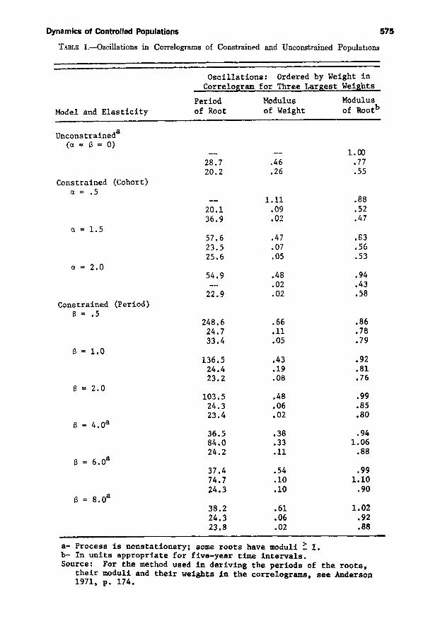
Table 1 shows the periods of the rootsof the characteristic polynomials, theirmoduli, and their weights in the correlo­gram for each model (for the methodused to derive these, see Anderson, 1971).The roots are ranked according to theirweights, and only the three most im­portant are shown. We note that theuncontrolled model has a root with unitmodulus and is hence nonstationary.Otherwise nonstationarity due to explo­sive oscillations arises from high controlelasticities (e.g., for values of 13 abovetwo).

Our major interest is in the dominantperiodicities and the way in which theyare affected by control. For the uncon­trolled model (ex = 13 = 0) there is onlya generational cycle, with period roughlyequal to the mean age of the net ma­ternity function. This corroborates theresults of previous deterministic analy­ses. For the cohort-controlled model witha control elasticity (a) of .5, the genera­tional cycle virtually disappears, and thecorrelogram is dominated by an expo­nential decline to zero, indicated by thereal root. This is entirely consistent withthe two-age-group model with 1 < as <2. For the cohort-controlled model withcontrol elasticity greater than one, theprocess exhibits a control cycle of twogenerations length, and the generationalcycle is of little importance. Thus in thiscase also, the two-age-group model pro­vides an accurate representation of thedynamics.

The behavior of the period control

model (which we prefer) is much morecomplicated. For control elasticities (13)less than one, there is a very long controlcycle of well over a hundred years; andsuperimposed on it is a modified genera­tional cycle of about twenty-five years.As the elasticity increases, the controlcycle period becomes steadily shorterand loses importance relative to themodified generational cycle. At 13 = 4,which is unstable, the process is domi­nated by fluctuations of 36.5 and 84.5years. Above this elasticity, the controlcycle and generational cycle merge at aperiod of about thirty-eight years, whichdominates all else. We note that withthe period model the elasticity must bevery high to produce a control cycle neartwo generations in length; and when ashort control cycle does emerge, its pe­riod is substantially less than two gen­erations. The two-age-group model nolonger provides a satisfactory simplifi­cation.

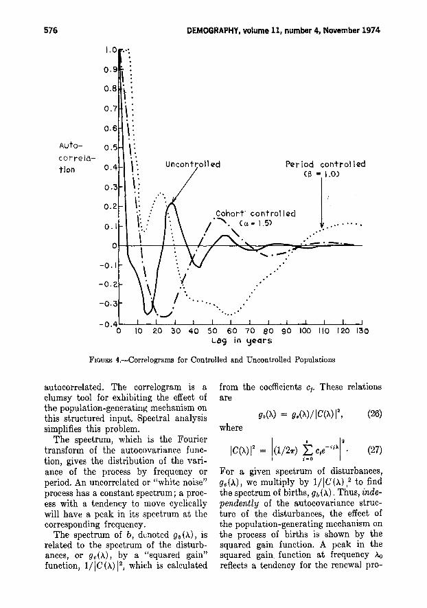
We now consider Figure 4, which showsseveral theoretical correlograms. For theuncontrolled model, the pseudo-correlo­gram shows sharply damped oscillationsof about twenty-eight years length, asexpected. The correlogram for ex = 1.5shows a damped 57.6-year cycle andconforms closely to the correlogram of afirst-order Markov process with ri =- .37 and time measured in twenty-eight­year units. The correlogram for the pe­riod model with 13 = 1 shows a 24.4-yeargenerational cycle superimposed on a136-year control cycle.

As we have mentioned, the correlo­gram interests us because its oscillationsreflect a tendency for the process to os­cillate with the same periodicity. How­ever, the correlogram depends not onlyon the coefficients OJ but also On the auto­correlation structure of the disturbanceterm, e, which we have implicitly as­sumed to be serially uncorrelated. Infact, however, disturbances reflect eco­nomic, meteorological and epidemeolog­ical conditions, each of which is itself

Dynamics of Controlled Populations

TABLE i.-Oscillations in Correlograms of Constrained and Unconstrained Populauons

a- Process is nonstationary; some roots have moduli ~ 1.b- In units appropriate for five-year time intervals.Source: For the method used in deriving the periods of the roots,

their moduli and their weights in the correlograms, see Anderson1971, p. 174.

575

576 DEMOGRAPHY, volume 11, number 4, November 1974

1.0 .,~

"

"....

. '--'-'

Period controlled

ce lO' .....,,'

Cohor-t' co nt rol led;' '"' , Cex • 1.5)

. "

uncontroll ed

-0.3

0.9 \

0.8 \ :0.7 \:. ,

0.6 \:. ,

Auto- 0.5 \:cor rele- , '

flon 0.4 r.0.·3 \:

"

0.2 \:0.1

\\ :,:....

0\\

-0.1\

-0.2\

- 0 .4'----L_--'-_-1-_J----'_-J.._-'-_..1.---'L...-........_~_...I____J

o 10 20 30 40 50 60 70 80 90 100 110 120 130Lag in \jeers

FIGURE 4.-Correlograms for Controlled and Uncontrolled Populations

autocorrelated. The oorrelogram is aclumsy tool for exhibiting the effect ofthe population-generating mechanism onthis structured input. Spectral analysissimplifies this problem.

The spectrum, which is the Fouriertransform of the autocovariance func­tion, gives the distribution of the vari­ance of the process by frequency orperiod. An uncorrelated or "white noise"process has a constant spectrum; a proc­ess with a tendency to move cyclicallywill have a peak in its spectrum at thecorresponding frequency.

The spectrum of b, denoted gb (A), isrelated to the spectrum of the disturb­ances, or ge(A), by a "squared gain"function, 1/IC(A) 12 , which is calculated

from the coefficients Ci' These relationsare

where

IC(>-)12 = 1(1/2'11) ~Cje-ijXr, (27)

For a given spectrum of disturbances,ge (A), we multiply by 1/ IC (A) 1

2 to findthe spectrum of births, gb (A). Thus, inde­pendently of the autocovariance struc­ture of the disturbances, the effect ofthe population-generating mechanism onthe process of births is shown by thesquared gain function. A peak in thesquared gain function at frequency Aoreflects a tendency for the renewal pro-

Dynamics of Controlled Populations

cess to create cycles of frequency x, andperiod l/Ao, out of random disturbance.When the disturbance term, e, is seriallyuncorrelated, then its spectrum is a hori­zontal line, and the squared gain func-

577

tion represents exactly the shape of thespectrum of births.

Figure 5 plots squared gain againstfrequency for the cohort-controlled modelwith various elasticities, a, including zero

10090807060

50

40

30

987

.~54.5 years

I~i \..I \

II,I

2 3 4 5 6

Cycles per centurlj

FIGURE 5.-Squared Gain for the Cohort Model

o

3

2

109876

5

4

1.0f--4-#---~1-----~~~~=~"!:30_-----.9

F.8.7.6

.5

s9u~red 20Gain

578 DEMOGRAPHY, volume 11, number 4, November 1974

(no control). We see that the uncon­trolled population amplifies variation atperiods of about twenty-eight years, andalso at very long periods (low frequen­cies). (For a much more detailed discus­sion of the squared gain of an uncon­trolled population in a nonstochasticcontext, see Coale, 1972.) This ampli­fication at long periods reflects the ab­sence of control; when fertility remainsabove equilibrium for a long time, thebirth series will grow exponentially with­out restraint. The effect of cohort con­trol with elasticities (a) less than oneis to flatten out the spectrum and reducethe generational cycle, or echo. Note inparticular that low frequency (long pe­riod) fluctuations are drastically reducedin amplitude, which is the expected effectof control. When the elasticity is aboveone, there is an amplification of varianceat periods of two generations; the echodisappears and is replaced by a controlcycle.

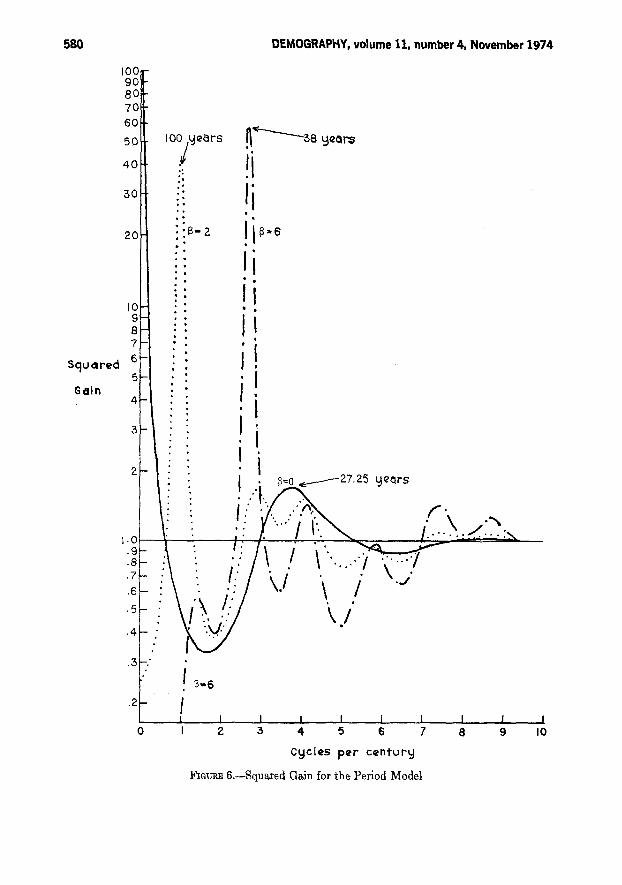
Figure 6 shows the inverse squaredgain for f3 = 2 and 6 in the period model.At f3 = 2, there is a very strong controlcycle with a period of one hundred years,which swamps the generational cycle,represented by two small peaks. Whenf3 =6, there is a very strong control cyclewith period thirty-eight years. For thismodel also, we note the attenuation ofall low frequency variations, in sharpcontrast to the uncontrolled model whichamplifies them.

Let us recapitulate the main results ofthis part. The dynamics of controlledpopulations, are, indeed, quite differentfrom those of uncontrolled populations,at least for moderately high control elas­ticities. Uncontrolled populations tend tofluctuate with a period of one generation.In cohort-controlled populations, evenwith low elasticities, the importance ofthis generational cycle is sharply re­duced. When the control elasticity ex­ceeds one, the generational cycle dis­appears altogether and is replaced by acontrol cycle twice as long. This latterresult is sufficiently strong and un-

ambiguous to permit inference from ob­served dynamics to the presence orabsence of strong control, provided thecohort model is an appropriate specifica­tion. We believe, however, that theperiod-control model is more reasonable.And unfortunately the dynamics of thismodel are more complicated and provideless clearcut indications. For low elas­ticities, the generational cycle remains,superimposed on a very long controlcycle of over a century. At very highelasticities there is a single cycle withperiod less than two generations; butbefore this appears, the system becomesunstable.

7. PRELIMINARY RESULTS FOR THE

UNITED STATES

The empirical analysis which is under­taken in this part is intended to be il­lustrative and suggestive, not a formaltest or demonstration. We begin with adiscussion of the correlogram of birthsfor the United States, 1900 to 1972, anda comparison of this correlogram withthe correlogram of baptisms for a pre­industrial French parish, 1590-1800. Wethen estimate the fertility relations as­sumed by each of the two models wedeveloped and consider whether the esti­mated relations are consistent with theobserved dynamic behavior.

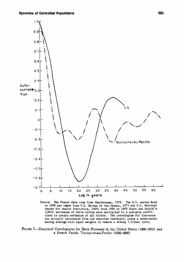
The correlograms for the United Statesand Tourouvre-au-Perche are shown inFigure 7. These are calculated from theproportional deviations of births fromexponential trend, estimated as the re­siduals from the regression of the logof annual births on time. Tourouvre waschosen arbitrarily from those parisheswith long published series. The correlo­gram for Tourouvre shows a twenty­nine-year cycle, which is also found,plus or minus a few years, in the otherthree parish baptism series I have ana­lyzed. The work of the previous sectionshows that these would be characteristicof uncontrolled or weakly controlledpopulations, though the possibility thatthese cycles are forced oscillations due

.812.

(29)

Dynamics of Controlled Populations

to climate or prices cannot yet be en­tirely ruled out. The fifteen-year cyclewhich the eorrelogram also reveals isalmost certainly due to a correspondingcycle in grain prices.

The correlogram for the United States,on the other hand, shows a strong peakat about thirty-nine years. Relative tothe hypothesized "cycle" length the seriesis much too short for accurate estima­tion. But taken at face value, the esti­mate conforms very closely to the pre­dicted cycle length of thirty-eight yearsgenerated by the period model with ahigh control elasticity. According to themodel (see Table 1), the oscillationsshould be explosive, but the empiricalcorrelogram cannot provide informationon this score.

We now consider the estimated fer­tility equations. The first model is basedon the assumption that period fertilityrates depend on the size of the (dis­counted) potential labor force, as inequation (17). To test this assumption,we first find the deviations of potentiallabor force size from exponential trendby calculating the residuals of the re­gression of the log of the population aged15 to 64 on time. (We use Potentialrather than actual labor force size, be­cause it is the base population size inrelation to available nonlabor inputswhich determines the feasible set of ag­gregate income-leisure choices for thesociety.) Then the log of the total fer­tility rate (equal to twice the sum of allthe ma,t for period t) is regressed on theseresiduals. The results are shown belowfor U. S. data, 1917 to 1972, aggregatedinto eleven observations of quinquennialaverages (the standard errors of the esti­mates are shown in parentheses) :

In (P/S-64)

= 11.102 + .01l4t + el , R 2 = .988;

(.0142) (.000419) (28)

In (TFR.)= 7.942 - 7.724e. + U" R 2

=

(.0247) (1.241)

579

We thus find a highly significant esti­mate of 7.7 for [3, and 80 percent of thevariance in fertility is "explained." When[3 actually has this value in the periodmodel, births tend to move in an explo­sive thirty-eight-year cycle. Thus, theestimated elasticity is strikingly consis­tent with the observed dynamic behavior,which helps to confirm the model. On theother hand, if this fluctuation in fer­tility were forced on the system by exo­genous factors, then we would necessarilyestimate a high, though spurious, elas­ticity [3. The consistency of the esti­mated [3 with the dynamic behavior cutsboth ways.

The second model is based on the as­sumption that cohort fertility rates aredependent on cohort size, as in equation(19). To test this hypothesis, we firstobtained the residuals from the regressionof the log of cohort size on time, as ameasure of the deviation of cohort sizefrom its stable growth path. We usedfive-year birth cohorts, 1890-1894 to1950-1954. The estimates given in equa­tions (30) .and (31) are based on cohortsize measured at ages 0-4. We found verysimilar results measuring cohort size atages ~24, which reflects changes inmigration and mortality, as well as insize at birth.

We then regressed the "completed" co­hort fertility on the residual from equa­tion (30). For many cohorts this in­volved some projection of fertility, butfor all except the last, which had borneonly about half its expected number ofchildren, this cannot have led to largeerrors. We followed Ryder (1971) forcohorts through 1919; after that we fol­lowed U. S. Bureau of the Census (1972).

The results are shown below:

In (Bl )

= 2.133 + .00902t + e., R2= .676;

(.0749) (.00188) (30)

In (TFR I )

= .966 - .954e. + U" R 2 = .710 .

(.0216) (.184) (31)

580

10090807060

50

40

30

20

109B7

Squdlred 6

'5Gain

4

3

2

1·0.9.8.7

.6

.5

.4

.3

.2

0

.'.'.'.'·.·.·.:'f3- 2·:·· .·.· .: .· .·.·.· .· .· .· .

DEMOGRAPHY. volume11, number4. November 1974

~~38 ~eo~

!i~ i!i~a6Iii i·.II· iI .· II .i ~· II .· II .-· :~. .

!/ .....·......I·:~( r: \ ."".' ......~ ... :

\. .' \....... ,,/ . '\..'/\/ " i .J

\j

cycles per century

FIGURE 5.-Squared Gain for the Period Model

Dynamics of Controlled Populations 581

1.0

504540

.,/ '. '\

r: /. '- .../'/

, /........ ' tcurouvre-eu-Perche

20 25 30 35

Lag in ~ears

1510

0.8 \0.7 \0.6 \0.5

\

\0.4

Auto- \correI4-0.3

\tion

0·2 \01 \

0 \

-0.1\

-0.2

-0.3

-0·4

-0.5

- 0.6

-0·70 5

Source: The French data come from Charbonneau, 1970, The U.S. series backto 1909 was taken from U.S. Bureau of the Census, 1973 and U.S. NationalCenter for }Lealth Statistics, 1969; from 1900 to 1909 Coale and Zelnik's(1963) estimates of white births were multiplied by a suitable coeffi­cient to obtain estimates of all births. The correlogram for Tourouvrewas actually calculated from the smoothed residuals, using a seven-pointmoving average with equal weights to remove a strong 7.S-year cycle.

FIGURE 7.-Empirical Correlograms for Birth Processes in the United States (1900-1972) anda French Parish, Tourouvre-au-Perche (1590--1800)

582 DEMOGRAPHY, volume 11, number 4, November 1974

This model also gives a good fit,though not so close as the previous one.However, in this case the estimated elas­ticity, - .954, is not consistent with thedynamic behavior of the system. Anelasticity of -1 would immediatelydamp any disturbance, and the expectednumber of births would be the same, re­gardless of cohort size. The model withthis estimated value of a is thus incapa­ble of generating the observed patternof fluctuation in births or fertility. Ap­parently, therefore, this version of themodel is inconsistent with the dynamicbehavior of population in the UnitedStates.

8. DISCUSSION

Two distinct kinds of cycles may arisein populations: the "generational" cycleor "echo" due to the intrinsic dynamicsof population renewal as an age-struc­tured process and the "control" cycledue to the lagged operation of equilibrat­ing mechanisms. In populations growingwithout effective constraint, such asmight occur temporarily in newly settledareas, only the generational cycle willarise. This case has previously been ana­lyzed in a deterministic context; we haveextended the analysis to a stochasticcontext and derived the theoretical cor­relogram and spectrum of the birth pro­cess. The cycles are shown to arise fromthe "filtering" of random variations bythe age structure of reproduction, ratherthan from the repercussions of a singledistorting shock. '

When homeostatic control is effectivelypresent, the pattern of fluctuation de­pends on the form of the control mech­anism and its sensitivity. We have con­sidered two kinds of mechanisms. In theperiod model, the labor supply exertsdownward pressure on welfare and fer­tility in each time period, while in thecohort model the size of each cohortaffects its welfare and fertility through­out its life.

When control is weak, the period

model continues to exhibit generationalcycles, although these are superimposedon a very long control cycle of one ortwo centuries periodicity. In the cohortmodel, no control cycle emerges, and thegenerational cycles are strongly damped.We conclude that, when control is weak,it will be difficult or impossible to drawconclusions about possible control froman analysis of population fluctuations; itwill be necessary to examine their long­run behavior.

When control is strong, the cohortmodel exhibits strikingly different be­havior; the generational cycle disappearsand is replaced by a control cycle oflength two generations. As the controlelasticity of the period model increases,it first becomes unstable and then de­velops a very strong thirty-eight-yearcycle. We conclude that at high controlelasticities either system would presentsufficiently distinctive dynamics to berecognizable.

Preliminary empirical analysis sug­gests that only the generational cyclewas prominent in preindustrial Europe.This would indicate relatively low con­trol elasticities, which is consistent withthe low long-run elasticity estimated forpreindustrial England by Lee (1970,1973, 1974b). But in the nineteenth cen­tury, dominated by the Kondratieff longcycle, the generational cycle is conspicu­ously absent. Thus the correlogram ofthe birth series for nineteenth-centuryFrance (not shown in this paper) has asingle strong peak at fifty-five years.And in the twentieth century, the UnitedStates, relatively undisturbed by war,has a single and very strong peak in itsbirth correlogram at thirty-nine years.Might these longer fluctuations representcontrol cycles? Is it possible that thelaws of motion for demographic pro­cesses underwent a radical change withindustrialization and/or the transition tolower fertility? Are the populations ofmodern industrial nations, far fromgrowing out of control, actually subject

(A.8)

Dynamics of Controlled PopulatiOns

to a more sensitive regulation than theirpreindustrial predecessors? These arehighly speculative hypotheses, based onthe slenderest evidence, but they invitefurther investigation.

ApPENDIX

Analysis of a Growing System

We have developed and analyzed amodel of population renewal under theassumption that the equilibrium popula­tion size was constant. We now supposethat the constraint to which the popu­lation is subject is receding at a constantrate u, as the result of capital accumula­tion, technical change, increasing qualityof labor, or other unspecified factors.Then the population size which is con­sistent with any given level of welfareis increasing at rate u. To illustrate forthe model of section 2, without age struc­ture, we would have U', = U'(e-u,p,) .

We may also suppose that the relationbetween fertility and welfare is chang­ing with time at some constant rate v,due to rising expectations; then the levelof welfare necessary to induce a givenlevel of fertility increases at a rate v. Inthe model without age structure, wewould have b, = b(e--v'U',). The systemwill have a steady state growth rate rfor population, which will depend on therates u and v and on the functiondetermining U'.

Now let us consider the more generalage-structured model of section 4. Let rdenote the steady state growth rate ofpopulation and of births resulting fromthe interplay of changes in productivityand in expectations. When the stream ofbirths grows at rate r, the net maternityfunction will be constant. The net ma­ternity function, then, may be writtenas follows:

¢a.,(B,)

- A. [e-r<c-IlB . . . -r<C-w)B 1- '/'0 '-I" e c-,. ,

(A.l)

583

or, to slightly extend our earlier notation,

ePa.,(B,) = ePo(e-r'B,). (A.2)

The renewal equation based on (A.2) is

B, = L ePo(e-rIBc)B,_o. (A.3)

Now consider the transformed birthsequence, B,*, and the net maternityfunction, ePa* (B,*) , defined, respectively,as follows:

and

ePo*(B,*) = e-r°ePo(B,*). (A.5)

Substituting into the renewal equation(A.3) and dividing both sides by e:"we find

B,* = L ePo*(B,*)B,- o*' (A.6)

But this is precisely the equation ana­lyzed in section 4.

In section 6 we showed how to deter­mine the autocorrelation function and thespectrum for birth fluctuations in a con­strained system with a constant equi­librium, where fluctuations were meas­ured as proportional deviations of birthsfrom equilibrium. The analysis wasbased on coefficients (ePa + "1a) in equa­tion (15). Our discussion in this part ofthe Appendix has shown that the entireanalysis in section 6 carries over to agrowing system; we need only multiplyeach coefficient in (15) by e-ra and pro­ceed as before.

Derivation of the Linear Approximation

The linear approximation is given by

B, == B* + L (fJB,/fJB'_o)(B,_o - B*),(A.7)

where the partial derivatives are to beevaluated at equilibrium. These partialderivatives may be calculated from (12) I

yielding

fJB,/fJB,-o = ePo(B,)

+ L [fJeP;(B.)/fJB,-.]B,-i-

n; = (B*/1.0) (aRt/aBt-a) IB,-B>. (A.11)

It therefore follows from (A.9) that

DEMOGRAPHY, volume 11, number 4, November 1974

Chambers, J. D. 1972. Population, Economyand Society in Preindustrial England. Ox­ford: Oxford University Press.

Charbonneau, Hubert. 1970. Tourouvre-au­Perche Aux XVII" et XVIII" Siecles. Paris:Presses Universitaires de France.

Coale, Ansley. 1963. The Economic Effects ofFertility Control in Underdeveloped Areas.In Roy Greep (ed.), Human Fertility andPopulation Problems. Cambridge: Schenk­man Publishing Co.

--. 1972. The Growth and Structure ofHuman Populations: A Mathematical Inves­tigation. Princeton: Princeton UniversityPress.

--, and Melvin Zelnik. 1963. New Esti­mates of Fertility and Population in theUnited States: A Study of Annual WhiteBirths from 1855 to 1960 and of Complete­ness of Enumeration in the Censuses from1880to 1960. Princeton: Princeton UniversityPress.

Davis, Harold T. 1963. The Analysis of Eco­nomic Time Series (reissued ed.). San An­tonio: Principia Press of Trinity University.

Easterlin, Richard. 1962. The American BabyBoom in Historical Perspective. Occasionalpaper no. 79. New York: National Bureaufor Economic Research.

--. 1968. Population, Labor Force, andLong Swings in Economic Growth. NewYork: National Bureau for Economic Re­search.

--, and Gretchen Condran. 1974. A Noteon the Recent Fertility Swing in Australia,Canada, England and Wales, and the UnitedStates. In Migration, Foreign Capital andEconomic Development: Essays in Honor ofBrinley Thomas. Forthcoming.

Goubert, Pierre. 1965. Recent Theories andResearch in French Population between 1500and 1700. Pp. 457-473 in D. V. Glass andD. E. C. Eversley (eds.). Population in His­tory. Chicago: Aldine Publishing Co.

Grauman, John. 1960. Comment. In NationalBureau for Economic Research (ed.), Demo­graphic and Economic Change in DevelopedCountries. Princeton: Princeton UniversityPress.

Howrey, P. E. 1968. A Spectrum Analysis ofthe Long-Swing Hypothesis. InternationalEconomic Review 9 :228-252.

Keyfitz, Nathan. 1965. Estimating the Trajec­tory of a Population. Proceedings of theFifth Berkeley Symposium on MathematicalStatistics and Probability 4 :81-113.

__. 1968. Introduction to the Mathematicsof Population. Reading: Addison-Wesley.

__. 1972. Population Waves. Pp, 1-38 inT. N. E. Greville (ed.). Population Dynam­ics. New York: Academic Press.

(A.12)

(A.l4)

REFERENCES

Evaluated at equilibrium, this is

584

L: ar/>;(B,)/OBt-a = aRt/aBt-a, (A.lO)

and in equilibrium R equals one. Theelasticity at equilibrium of R, with re­spect to Bt-a, which we denote 7Ja, there­fore is given by

aBt/OBt-a IB,-B> = r/>a + 1/a,

and hence from (A.7) that

Anderson, T. W. 1971. The Statistical Analysisof Time Series. New York: John Wiley &Sons.

Birdsell, Joseph. 1957. Some Population Prob­lems Involving Pleistocene Man. ColdSprings Harbor Symposia on QuantitativeBiology 22:47-69.

Bernardelli, Harre. 1941. Population Waves.Journal of the Burma Research Society31 :1-18.

aBt/aBt-a = r/>a + B*

..l: ar/>;(Bt)/aBt-a IB,-B>. (A.9)

Now by definition of R, we have

ACKNOWLEDGMENTS

The research on which this paper isbased was supported by the PopulationStudies Center of the University ofMichigan. Professors Saul Hymans andPhil Howrey and two referees made use­ful comments on an earlier draft. Theauthor gratefully acknowledges the re­search assistance of Martha Hill andDavid Levinson and the typing andpreparation of diagrams by CarolynCopley.

B, == B* + L: (r/>a + 1/a)(Bt-a - B*).

(A.l3)

Finally, letting bt = iB, - B*)/B*,(A.l3) implies that

Dynamics of Controlled Populations

Le Bras, Herve. 1969. Retour d'une popula­tion a l'etat stable apres une "catastrophe."Population 24:861--s96.

--. 1971. Elements pour une theorie despopulations instables. Population 26:525-572.

Lee, Ronald. 1970. Econometric Studies ofTopics in Demographic History. Unpub­lished Ph. D. dissertation. Cambridge: Har­vard University.

--. 1973. Population in Preindustrial Eng­land: An Econometric Analysis. QuarterlyJournal of Economics 87:581--Q07.

--. 1974a. Forecasting Births in Post-Tran­sition Populations: Stochastic Renewal withSerially Correlated Fertility. Journal of theAmerican Statistical Association 69:607-617.

--. 1974b. Models of Preindustrial Popu­lation Dynamics with Applications to Eng­land. In Charles Tilly (ed.), Early Indus­trialization, Shifts in Fertility and Changesin Family Structure. Forthcoming. Prince­ton: Princeton University Press.

Leibenstein, Harvey. 1963. Economic Back­wardness and Economic Growth. New York:John Wiley & Sons.

Liu, Paul. 1971. Marshall's Economic Theoryof Population. Unpublished manuscript. EastLansing: Department of Economics, Michi­gan State University.

Malthus, Thomas Robert. 1970. An Essay onthe Principle of Population (1798). Editedby Anthony Flew. Baltimore: PenguinBooks Inc.

Pearl, Raymond. 1924. Studies in Human Biol­ogy. Baltimore: Williams & Wilkins.

Pollard, J. H. 1973. Mathematical Models forthe Growth of Human Populations. Cam­bridge: Cambridge University Press.

Ryder, Norman B. 1971. The Time Series ofFertility in the United States. In Interna-

585

tional Union for the Scientific Study ofPopulation (ed.), International PopulationConference, London, 1969. Vol. 1. London:International Union for the Scientific Studyof Population.

Sauvy, Alfred. 1969. General Theory of Popu­lation. New York: Basic Books.

Solow, Robert. 1956. A Contribution to theTheory of Economic Growth. QuarterlyJournal of Economics 79:65-94.

Simon, Julian L. 1974. The Effects of Incomeon Fertility Control. Chapel Hill: CarolinaPopulation Center.

U. S. Bureau of the Census. 1972. Projectionsof the Population of the United States, byAge and Sex: 1972 to 2020. Current Popula­tion Reports, Series P-25, No. 493. Washing­ton, D. C.: Government Printing Office.

--. 1973. Statistical Abstract of the UnitedStates: 1973. Washington, D. C.: Govern­ment Printing Office.

U. S. National Center for Health Statistics.1969. Vital Statistics of the United States:1967. Vol. 1. Natality. Washington, D. C.:Government Printing Office.

Winsborough, H. H. 1974. Age, Period, Cohortand Education Effects on Earnings by Race.In Kenneth Land and Seymour Spilerman(eds.), Social Indicator Models. Forthcoming.New York: Russell Sage Foundation.

Wray, Joe D. 1971. Population Pressure onFamilies: Family Spacing. In National Acad­emy of Sciences (ed.), Rapid PopulationGrowth: Consequences and Policy Implica­tions. Baltimore: Johns Hopkins Press.

Wrigley, E. A. 1969. Population and History.New York: McGraw-Hill.

Yule, G. Udney. 1906. Changes in the Marriageand Birth Rates in England and Wales Dur­ing the Past Half Century. Journal of theRoyal Statistical Society 69:18-132.