The Fractured Nature of British Politics Carlos Molinero * , Elsa Arcaute , Duncan Smith , and Michael Batty Centre for Advanced Spatial Analysis (CASA) University College London (UCL) June 7, 2021 Abstract The outcome of the British General Election to be held in just over one week’s time (May 7th, 2015) is widely regarded as the most difficult in living memory to predict. Current polls suggest that the two main parties (Conservative and Labour) are neck and neck but that there will be a landslide to the Scottish Nationalist Party with that party taking most of the constituencies in Scotland (some 50 out of 59 on the most recent forecast for Sunday April 26th). The Liberal Democrats are forecast to loose more than half their seats (56 to 24) and the fringe parties of whom the UK Independence Party is the biggest are simply unknown quantities. Much of this volatility relates to long-standing and deeply rooted cultural and nationalist attitudes that relate to geographical fault lines that have been present for 500 years or more but occasionally reveal themselves, at times like this. In this paper our purpose is to raise the notion that these fault lines are critical to thinking about regionalism, nationalism and the hierarchy of cities in Great Britain (excluding Northern Ireland). We use a percolation method [1] to reveal them that treats Britain as a giant cluster of related places each defined from the intersections of the road network at a very fine spatial scale (down to 50 metre resolution). We break this giant cluster into a detailed hierarchy of sub-clusters by successively reducing a distance threshold starting at 5 kilometres which first breaks off some of the Scottish Islands and then reveals the very distinct nations and regions that make up Britain, all the way down to the definition of the largest cities that appear when the threshold reaches 300 metres. We use these percolation clusters to apportion the 2010 voting pattern to a new hierarchy of constituencies based on these clusters, and this gives us a picture of how Britain might vote on purely geographical lines. We then examine this voting pattern which provides us with some sense of how important the new configuration of political parties might be to the election next week. * Corresponding author [email protected]; [email protected]; [email protected]; [email protected]1 arXiv:1505.00217v1 [physics.soc-ph] 1 May 2015
Transcript
The Fractured Nature of British Politics
Carlos Molinero∗, Elsa Arcaute , Duncan Smith , and Michael Batty
Centre for Advanced Spatial Analysis (CASA)University College London (UCL)
June 7, 2021
Abstract
The outcome of the British General Election to be held in just over one week’stime (May 7th, 2015) is widely regarded as the most difficult in living memory topredict. Current polls suggest that the two main parties (Conservative and Labour)are neck and neck but that there will be a landslide to the Scottish Nationalist Partywith that party taking most of the constituencies in Scotland (some 50 out of 59 onthe most recent forecast for Sunday April 26th). The Liberal Democrats are forecastto loose more than half their seats (56 to 24) and the fringe parties of whom theUK Independence Party is the biggest are simply unknown quantities. Much ofthis volatility relates to long-standing and deeply rooted cultural and nationalistattitudes that relate to geographical fault lines that have been present for 500 yearsor more but occasionally reveal themselves, at times like this. In this paper ourpurpose is to raise the notion that these fault lines are critical to thinking aboutregionalism, nationalism and the hierarchy of cities in Great Britain (excludingNorthern Ireland). We use a percolation method [1] to reveal them that treatsBritain as a giant cluster of related places each defined from the intersections of theroad network at a very fine spatial scale (down to 50 metre resolution). We breakthis giant cluster into a detailed hierarchy of sub-clusters by successively reducinga distance threshold starting at 5 kilometres which first breaks off some of theScottish Islands and then reveals the very distinct nations and regions that makeup Britain, all the way down to the definition of the largest cities that appear whenthe threshold reaches 300 metres. We use these percolation clusters to apportionthe 2010 voting pattern to a new hierarchy of constituencies based on these clusters,and this gives us a picture of how Britain might vote on purely geographical lines.We then examine this voting pattern which provides us with some sense of howimportant the new configuration of political parties might be to the election nextweek.
Long-standing cultural differences between the countries that comprise the United King-dom are part of the folklore of British politics but in the last twenty-five years they havereasserted themselves with a vengeance. The devolution of central powers from the gov-ernment in Westminster to Scotland and Wales were first initiated a generation ago whileNorthern Ireland has had periods from the 1970s when its traditional parliament, nowassembly, has been entirely suspended. However these divisions have not really assertedthemselves in terms of national voting until the last decade but it now looks as thoughBritain in its forthcoming general election on 7th May 2015 will finally divide itself alongvery deep and historically significant lines.
In recent times, since the 1960s, the traditional two party system that had dominatedpolitics since the early 20th century began to slowly fracture with the Liberals (now Lib-eral Democrats) reasserting themselves in south west England while also making inroadsinto somewhat conservative but relatively high income city suburbs and country towns.The Scottish Nationalist Party (SNP) began to gain more seats after devolution and re-cent local and European elections have led to a massive increase in their support that iswidely seen as a sea change in the quest for Scottish independence. The SNP are forecastto more or less wipe out the traditional Labour Party in Scotland in the forthcominggeneral election. The Welsh nationalists Plaid Cymru have a much smaller base in Walesalthough it is entirely possible that they will gain seats in May while in Northern Irelandthe traditional focus on conservatism and nationalism has led to a split with the Conser-vative Party in England to which it is traditionally allied. Northern Ireland politics havebecome much more inward looking.
The two parties that have dominated national politics until quite recently the Con-servatives (the Tories) and the Labour party have also changed. The Blair and Browngovernments, from 1997 to 2010, introduced the philosophy that was called New Labour,with the party much more geared to contemporary business ethics and deregulation.There has been a substantial reaction against this with the party reverting to a some-what more traditional stance but like the present coalition of Conservatives and LiberalDemocrats espousing a pro-austerity stance in the wake of the Great Recession. TheLiberals, of course, joined with the Conservatives in 2010 in a coalition, the first longlasting one for well over 70 years, and this has softened and blurred traditional thinkingamongst the Conservatives and perhaps hardened and confused the philosophy of theLiberal Democrats. Add to this the emergence of the anti immigration and anti Euro-pean Union party, UKIP (the United Kingdom Independence Party) and the picture atfirst sight appears more confused that at any time since the Labour Party began to erodesupport for the Liberals in the late 19th century.
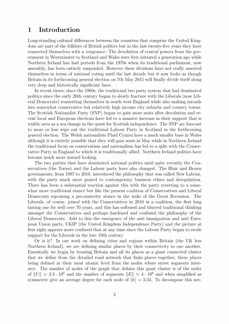
Or is it? In our work on defining cities and regions within Britain (the UK lessNorthern Ireland), we are defining similar places by their connectivity to one another.Essentially we begin by treating Britain and all its places as a giant connected clusterthat we define from the detailed road network that links places together, these placesbeing defined at their most atomic level from the nodes where street segments inter-sect. The number of nodes of the graph that defines this giant cluster is of the orderof ‖V ‖ ' 3.3 · 106 and the number of segments ‖E‖ ' 4 · 106 and when simplified assymmetric give an average degree for each node of 〈k〉 = 2.34. To decompose this net-
2
work into clusters with different degrees of connectivity, we begin by specifying a rangebased on the maximum segment length in the network, gradually relaxing this threshold,thus producing a hierarchy of clusters which is a unique decomposition of the Britishgeographical space. Note that we use street intersections as the basis for our definition ofany spatial unit so a parliamentary constituency, an area for which a politician is elected,is regarded as all the nodes and segments that fall uniquely into the physical area definingthat space.
The percolation method developed in [1] starts with the entire cluster, setting thestarting threshold at d = 5000m and the hierarchy of clusters emerges as we successivelyreduce this value. As we might expect from a casual knowledge of Britain, the moreremote periphery will disconnect first but we are not able to anticipate the actual parti-tioning. When the threshold reaches 1.4 km, Scotland breaks off completely from the restof England and Wales. The break is very geographically distinct, with the central low-lands dividing the country entirely from England excluding a few of the English bordercounties in the south. When the threshold falls to 900m, the Industrial North and Westand Wales separates off from the South East and then, when it falls another 100 metres,the South West and South Wales become distinct from this division. The big cities thenfall out of this when the threshold falls to 300 metres. The hierarchy is so clear that it ishard not to conclude without knowing anything else about these regions, that they areculturally and economically quite distinct. In the light of the debate about Scottish in-dependence and recent European election results, the geographical correlations with thepredominant voting patterns are surprising and very clear. The influence of geographicalboundaries on voting dynamics has already been studied in a few papers in the literature[2, 3, 4] but the notion of percolation and the way that it divides the geographical spacevastly improves our understanding on the matter and allows us to quantify those geo-graphical units in an univocal manner. Although there are many explorations of votingbehaviours using physical concepts particularly in opinion dynamics and voting structure[5], and many that have used the concept of percolation applied to consensus decisionmaking [6, 7, 8] and even studied the spread of opinions through networks [9, 10], none,as far as we are aware, are using a geographical percolation to explain voting patterns.
To get an immediate idea of this kind of clustering, we refer you to our percolationmovie where we successively partition the space by increasing the distance thresholdsystematically. Figure 1 shows the partition produced by the percolation at the thresholdsthat produce the most relevant divisions (300m, 800m, 900m, 1400m, 5000m).
If we were to suggest that the Scottish cluster coincided with predominant SNP voters,the south west with Liberal Democrats, the industrial north with Labour, and the southeast and shire counties with Conservatives, then one would not be far of the mark inwhat people have speculated this last six months about the forthcoming May election.UKIP do not show up in this physical decomposition and Wales blurs in the northernand western clusters for Plaid Cymru is largely a rural party, remote even within Wales.The local effects in urban areas where inner cities are more likely to vote Labour and thesuburbs Conservative are picked up when we go down to the much finer city thresholds.It is this that encourages us that using percolation to detect the degree of isolationismas well as the strong concentration in the British population space of orientation andnearness to other areas are remarkably strong determinants of what people will vote.
Figure 1: Network percolations at the main thresholds, respectively, 300m,800m, 900m, 1400m and 5000m . To view the animated sequence ofpercolation distances please refer to: http://www.mechanicity.info/
percolation-clustering-of-the-uk-road-network/.
2 Clustering of the percolation
2.1 Preliminary definitions
Let I be the set of intersections of the road network of Britain and let C be a set ofparliamentary constituencies with n being the number of constituencies. Each Ci ⊂ Cis a set of intersections that belong to the i-th constituency such that
⋃ni=1Ci = C,
Ci ∩ Cj = ∅ for all i and j and⋃n
i=1x | x ∈ Ci = I.For each constituency Ci we have a vector of voting behavior ~vi = (vi,1, · · · , vi,l) which
is composed of l elements, being l the number of political parties. We will refer to the k-thelement of the vector ~vi as vi,k, which is equal to the number of votes that the politicalparty k received in the constituency i.
2.2 Obtaining the percolation clusters
The technique to generate the percolation clusters is explained in detail in [1]. We willexplain in the following paragraphs a summarised version of the technique to performa network percolation, how it serves to generate a tree of the percolations, and how wecan use that tree to assign a unique cluster for each intersection of the road network ofthe UK. Given a graph of the road network, where nodes represent intersections and theweight for each edge is the length of the street that connects them and a certain metricthreshold (e.g. 5000m) we produce a network percolation by:
1. Selecting the transition of the graph with the smallest weight (distance), generatinga new cluster and inserting both its nodes into the cluster.
2. We will keep a first-in first-out queue of nodes to expand, from which we will extracta node to continue the process. We add both nodes of the transition selected instep 1 to this queue. Nodes are only added to this queue if they are not alreadyincluded.
3. Extract a node from the queue of nodes to explore and if a transition departing fromthat node (not yet included in the cluster) is smaller than the threshold, include thetransition in the cluster and the end node of the transition in the queue of nodesto explore.
4. Repeat step 3 until no further node can be expanded (the queue is empty) and ifthere are transitions left in the graph that do not belong to any cluster, generate anew cluster by choosing the smallest available transition and repeat from step 1.
This procedure will cover the complete graph with clusters, most of them irrelevantclusters of only a few nodes. To avoid this noisy behaviour we set a minimum size for acluster of 75 nodes in order to include it in the set of percolation clusters.
If we repeat this algorithm for a large set of distance thresholds (in the interval[5000, 50] every 50m), the largest distance will produce one single cluster for the wholeof the UK that includes every intersection. The following distance will produce a set ofsmaller clusters completely contained in the previous one, leaving behind a few intersec-tions. In fact, we can generate a tree of the percolation in this manner which renders theresult portrayed in Figure 2.
The set P of percolation clusters is the extended set that includes every cluster inthis tree with m being the number of percolation clusters. Each Pj ⊂ P is a set ofintersections that belong to the j-th percolation cluster such that
⋃mj=1 Pj = P and⋃m
j=1x|x ∈ Pj = I. The set P is not a disjoint set, meaning that the same intersectionwill belong to several percolation clusters simultaneously as long as they have a parent-son relationship. That is, given two percolation clusters Pj and Pk, Pj ∩ Pk 6= ∅ if thereexist a path in the percolation tree from Pj to Pk (or viceversa) and otherwise Pj∩Pk = ∅.
Figure 2: To the left, the complete tree of the percolation using all the calculated thresh-olds and every cluster larger than 75 nodes. To the right, a simplified version of thepercolation tree, generated by using only some selected thresholds and the largest 10clusters per distance presented to improve the understanding of the approach.
5
We will define the operation of intersecting a constituency with the set of percolationclusters as the operation that returns a vector (~pi) with size m where each componentj of the vector is the number of intersections that belong to the intersection of Ci ∩ Pj.That is, Ci ∩ P = ~pi, pi,j = ‖x|x ∈ Ci ∩ Pj‖.
This operation serves to generate a vector for each constituency that determines itscomposition in terms of the percolation clusters and that in turn, will serve to cluster theconstituencies into similar behavioral groups according to the percolation.
2.3 Clustering the percolation clusters following the parliamen-tary constituencies subdivision
We will use the partitioning around medoids algorithm (PAM [11]) to cluster the vectors~pi using the chi-squared distance [12] between them. In more detail, the distance between
the constituencies Ci and Ck is d(~pi, ~pk) = 12
∑∀j
(pi,j−pk,j)2pi,j+pk,j
. This algorithm will cluster the
constituencies into different sets according to their composition of percolation clusters.We will call the set that holds this set of disjoint clusters A, where each componentAg ⊂ A is composed of several constituencies (Ag = Ci, Ck, · · ·) such that
⋃‖A‖g=1Ag = C
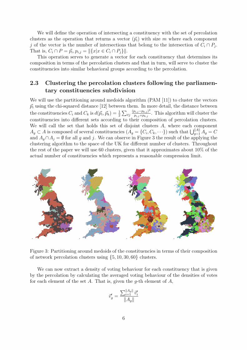
and Ag∩Aj = ∅ for all g and j. We can observe in Figure 3 the result of the applying theclustering algorithm to the space of the UK for different number of clusters. Throughoutthe rest of the paper we will use 60 clusters, given that it approximates about 10% of theactual number of constituencies which represents a reasonable compression limit.
Figure 3: Partitioning around medoids of the constituencies in terms of their compositionof network percolation clusters using 5, 10, 30, 60 clusters.
We can now extract a density of voting behaviour for each constituency that is givenby the percolation by calculating the averaged voting behaviour of the densities of votesfor each element of the set A. That is, given the g-th element of A,
~v′g =
∑‖Ag‖i=1 ~v′i‖Ag‖
6
where ~v′i = ~vi∑lj=1 vi,j
is the density vector of the voting behavior of the i-th constituency
belonging to the set Ag.
2.4 Performance of the clustering
In order to quantify the quality of the partitioning of the constituencies set based onthe percolation, we will study the error that it generates in comparison with severalother types of partitioning. On one side, we will take into account several socio-economicvariables from the 2011 census [13] that could be relevant to the voting behaviour such asthe degree of educational level (qualifications), the occupational class data (which servesas well as a proxy for income data), the age structure of the population and the countryof birth (that can account for areas with a strong immigration rate).
The data of the different variables is normalized by the total number of people thateach variable accounts for. Qualifications is a vector with 5 categories: no-qualification,level 1, 2, 3 and 4. Occupational data is a vector that distinguishes between Managers,Professional, Associate Professional, Admin, Skilled Trades, Other Service, Sales, Processand Elementary. Age structure is another vector that has separated into components thenumber of people in each age group segregated by periods of 5 years and country of birthdistinguishes between the categories UK, Ireland, Other EU, Other EU Accession andRest of the World. We will later use the same partitioning mechanism to produce theclustering of the constituencies.
As we can observe in Figure 4, the best clustering corresponds to the percolation,with the second best being occupational class data and the qualification variable whichperforms similarly. This shows how relevant it is the area to which one belongs, the levelof connectivity that it has to other regions and how deep in the percolation tree a regionis (cities have a larger depth than rural areas) to characterize voting behaviour. Thiscan be explained relatively easy by considering the role that the inter-exchange of ideasbetween peers has on cultural patterns and that areas that are highly connected (or evenbelong to the same region) will have a wider range of migrant flows thus influencing eachother’s way of thinking. The full extent of this analysis and how to be able to improvethe results by simultaneously using the socio-economic and the geographical data will betreated in future work.
In order to produce the plot, we will calculate the error as the sum of the distances be-tween the averaged voting vector of Ag (~v′g) and the voting behaviour of each constituencyCi (~vi) included in the set Ag. That is:
error =∑∀g,∀i
|wi · ~v′g − ~vi|
where wi =∑∀j vi,j is the total number of votes for constituency Ci.
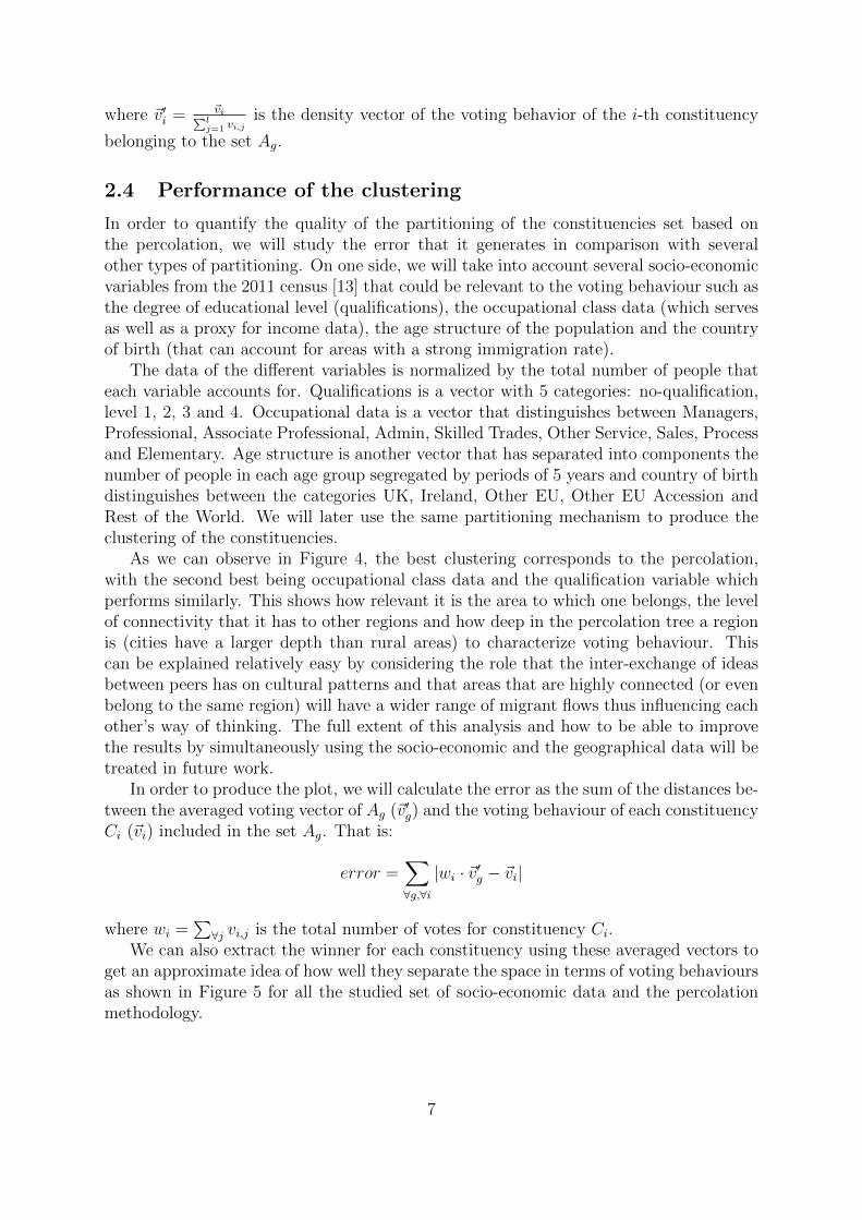
We can also extract the winner for each constituency using these averaged vectors toget an approximate idea of how well they separate the space in terms of voting behavioursas shown in Figure 5 for all the studied set of socio-economic data and the percolationmethodology.
7
Figure 4: Plot of the percentage of total error for different number of clusters in whichwe are comparing the socio-economic data with the approach presented in this paper.
2.5 Sub-trees
We have produced the tree of the percolation using the full set of percolation thresh-olds from 5000m to 50m, but we could perform this procedure calculating the clustersfrom 5000 to 4950 and generating the tree for those thresholds, gradually decreasing thelowest threshold generating different sub-trees of increasing detail. We could then studytheir clusterings and their averaged voting behaviour and measure how much error eachaccounts for.
Furthermore, we can produce the plot presented in Figure 6 for all the subtrees wherethe errors for the accumulated sub-trees are shown. In this Figure we can observe thatthere are 2 main thresholds where there are large decreases in the error thus producinglocal minima, exactly in the threshold of 1400 and in the 900, 800 range and in a smallerscale also in the 400, 300 range. Those 3 thresholds correspond respectively to 3 scales,the nation scale, the regional scale and the city scale that were represented in Figure 1.
3 Predicting voting behaviours
This entire approach is based on assuming that the percolation clusters identify a geo-graphical pattern from which voter behaviour can emerge as a consequence of nationalisticand regional attitudes that reflect how Britain is fracturing into its long standing histor-ical subdivisions. We should alert ourselves to the possibility that geographical factorsare more of a determinant of the current volatility in voter attitudes than at any time inthe last 100 years. To this end, we will examine how we might embed these geographicalconsiderations into a simple model that is able to predict votes by combining the 2010
8
Figure 5: From left to right, actual results of the winners from the 2010 elections; winnerextracted from the clustering based on the percolation; winner from the clustering of thequalifications variable; winner of the clustering from the occupational data; winners fromage structure clustering and country of birth clustering.
election results with our results from the percolation.In order to predict voting behaviour we use the the uniform national swing method [14]
segregated by Scotland and England with Wales, which takes the following form:
1. Using the votes vectors of the constituencies (~vi) we calculate the average votes foreach party in the two areas (Scotland and England with Wales).
2. Taking into account the percentages published in the polls by The New Statesmanof the final results (http://may2015.com) we produce a vector of swing votes fromScotland and England with Wales (~si for the constituency Ci).
3. Using both vectors we can generate a new vector of predicted votes for each con-stituency Ci as ~vpi = ~vi + ~si.
In order to have control values for our methodology we use the predictions presentedin http://www.electionforecast.co.uk/ which are shown in column AC of table 1and to ensure that our simple methodology is capable of generating valuable results, weproduce a prediction based on the actual votes (~vi) from the 2010 elections which is shownin column BP . As we can see in the table the results are quite similar.
We then proceed to apply this method to generate a prediction based on the per-colation. Instead of using the actual votes we use the averaged votes from the clustersgenerated with the percolation (~vi = wi · ~v′g) and recalculate the swing votes to form col-umn DP . Finally, we do the same for the clusters generated from the occupational datato generate column EP and later on, we calculate the average between the votes obtainedwith the percolation and the votes obtained with the occupational data, substitute vi torecalculate the swing votes and produce the output shown in column CP .
As we can observe, the result obtained with the percolation clusters overestimatethe impact of the Labour Party while the occupational data produces the inverse effect.
Figure 6: Errors of the accumulated subtrees for 60 clusters.
Using the average of both voting behaviours produces a map of constituencies that re-semble to a large extent the actual voting prediction showing that there is a underlyingrelationship between the voting patterns of people and their location in the network inclose relationship with the occupational data.
4 So What Will be the Outcome?
In essence, our model does not pick up either the extremes of voting that the currentpolls are showing, nor does it produce the neck and neck race between the traditionalparties. If the result of the election is as the recent YouGov polls suggest (see http:
Table 1: Voting predictions by number of seats. AC prediction from http://www.
electionforecast.co.uk/. BP Prediction based on the real voting vectors. CP pre-diction based on the percolation and the occupational class data voting behaviour. DP
prediction based on the percolation voting behaviour. EP prediction based in the occu-pational data.
Figure 7: From left to right: (BP ) Prediction using the actual votes and the polls; (CP )prediction by using the percolation and the occupational data; (DP ) prediction usingsolely the percolation; and (EP ) prediction using the occupational data.
//www.electionforecast.co.uk/) the Conservatives will gain 285 seats, Labour around270, the SNP 50 and the Liberal Democrats 25. This indeed would be a strange resultby historical standards. It probably represents a hung parliament with no party ableto win an outright majority and in fact no parties able to form a stable coalition. Theclosest that our model comes to forecasting this is with the Conservatives on 301, Labour271, the SNP 56 while the Liberal Democrats are erased from the map. But our mostextreme prediction which still takes account of the geographical effects produces a muchlarger concentration of seats for the Labour Party which brings up the topic of howcapable is the system of first pass the post to represent proportionally the number ofvotes taking into account that different partitioning of the constituencies produce verydifferent results. This variation is present as well in the opposite range by the partitiongenerated from the occupational data which agglomerate the constituencies in such a waythat the Conservatives get a clear win. Strange times indeed.
To an extent what we have developed here is a work in progress. We will only beable to refine our model, once the votes are known on May 7th 2015, when we will beable to undertake a much more considered analysis of geographical factors but we remainconvinced that geographical isolation, separation, and connectivity is a key factor indetermining not only how people vote but even how they think and it is this that wouldappear to be dictating the high volatility of current and more considered predictions.In fact in such a situation, there could well be a final bounce or shift, a transition totraditional or even more extreme or some combination of both when the voters take topolls and the votes are finally counted.
[1] E. Arcaute, C. Molinero, E. Hatna, R. Murcio, C. Vargas-Ruiz, P. Masucci, J. Wang,M. Batty, Hierarchical organisation of Britain through percolation theory (2015) 11,arXiv:1504.08318.
[2] R. Johnston, C. Pattie, Putting voters in their place: Geography and elections inGreat Britain, Oxford University Press, 2006.
[3] R. Johnston, C. Pattie, Geography: The Key to Recent British Elections, GeographyCompass (5) 1865–1880. doi:10.1111/j.1749-8198.2009.00258.x.
[4] T. Perez, J. Fernandez-Gracia, J. J. Ramasco, V. M. Eguıluz, Persistence in votingbehavior: Stronghold dynamics in elections, in: N. Agarwal, K. Xu, N. Osgood(Eds.), Social Computing, Behavioral-Cultural Modeling, and Prediction, Vol. 9021of Lecture Notes in Computer Science, Springer International Publishing, 2015, pp.173–181. doi:10.1007/978-3-319-16268-3\_18.
[5] J. Torok, G. Iniguez, T. Yasseri, M. San Miguel, K. Kaski, J. Kertesz, Opinions,Conflicts, and Consensus: Modeling Social Dynamics in a Collaborative Environ-ment, Physical Review Letters 110 (8) (2013) 088701. doi:10.1103/PhysRevLett.110.088701.
[6] D. Stauffer, Percolation and Galam Theory of Minority Opinion Spreading, In-ternational Journal of Modern Physics C 13 (07) (2002) 975–977. doi:10.1142/
S0129183102003735.
[7] J. Shao, S. Havlin, H. E. Stanley, Dynamic Opinion Model and Invasion Percolation,Physical Review Letters 103 (1) (2009) 018701. doi:10.1103/PhysRevLett.103.
018701.
[8] A. S. Balankin, M. A. Martınez Cruz, A. T. Martınez, Effect of initial concentrationand spatial heterogeneity of active agent distribution on opinion dynamics, PhysicaA: Statistical Mechanics and its Applications 390 (21-22) (2011) 3876–3887. doi:
10.1016/j.physa.2011.05.034.
[9] G. Travieso, L. da Fontoura Costa, Spread of opinions and proportional voting,Physical Review E 74 (3) (2006) 036112. arXiv:0603044, doi:10.1103/PhysRevE.74.036112.
[10] R. Lambiotte, M. Ausloos, J. A. Hoyst, Majority model on a network with communi-ties, Physical Review E 75 (3) (2007) 030101. doi:10.1103/PhysRevE.75.030101.
[11] H.-S. Park, C.-H. Jun, A simple and fast algorithm for K-medoids clustering, ExpertSystems with Applications (2) 3336–3341. doi:10.1016/j.eswa.2008.01.039.
[12] The quadratic-chi histogram distance family, in: K. Daniilidis, P. Maragos, N. Para-gios (Eds.), Computer Vision ECCV 2010, Vol. 6312 of Lecture Notes in ComputerScience, 2010. doi:10.1007/978-3-642-15552-9_54.
[13] Office for national statistics. 2011 census (2011).URL https://www.nomisweb.co.uk/census/2011
[14] R. J. Johnston, A. M. Hay, On the parameters of uniform swing in single-memberconstituency electoral systems, Environment and Planning A 14 (1) (1982) 61–74.doi:10.1068/a140061.