The Fundamentals of HTK - York University · The Fundamentals of HTK Training Tools Speech Data...

Chapter 1

The Fundamentals of HTK

Training Tools

Speech Data

Recogniser

Transcription

Unknown Speech Transcription

HTK is a toolkit for building Hidden Markov Models (HMMs). HMMs can be used to model anytime series and the core of HTK is similarly general-purpose. However, HTK is primarily designedfor building HMM-based speech processing tools, in particular recognisers. Thus, much of theinfrastructure support in HTK is dedicated to this task. As shown in the picture alongside, thereare two major processing stages involved. Firstly, the HTK training tools are used to estimatethe parameters of a set of HMMs using training utterances and their associated transcriptions.Secondly, unknown utterances are transcribed using the HTK recognition tools.

The main body of this book is mostly concerned with the mechanics of these two processes.However, before launching into detail it is necessary to understand some of the basic principles ofHMMs. It is also helpful to have an overview of the toolkit and to have some appreciation of howtraining and recognition in HTK is organised.

This first part of the book attempts to provide this information. In this chapter, the basic ideasof HMMs and their use in speech recognition are introduced. The following chapter then presents abrief overview of HTK and, for users of older versions, it highlights the main differences in version2.0 and later. Finally in this tutorial part of the book, chapter 3 describes how a HMM-basedspeech recogniser can be built using HTK. It does this by describing the construction of a simplesmall vocabulary continuous speech recogniser.

The second part of the book then revisits the topics skimmed over here and discusses each indetail. This can be read in conjunction with the third and final part of the book which providesa reference manual for HTK. This includes a description of each tool, summaries of the variousparameters used to configure HTK and a list of the error messages that it generates when thingsgo wrong.

Finally, note that this book is concerned only with HTK as a tool-kit. It does not provideinformation for using the HTK libraries as a programming environment.

2

1.1 General Principles of HMMs 3

1.1 General Principles of HMMs

s1 s2 s3 etc

s1 s2 s3

SpeechWaveform

SpeechVectors

Concept: a sequence of symbols

Parameterise

Recognise

Fig. 1.1 MessageEncoding/Decoding

Speech recognition systems generally assume that the speech signal is a realisation of some mes-sage encoded as a sequence of one or more symbols (see Fig. 1.1). To effect the reverse operation ofrecognising the underlying symbol sequence given a spoken utterance, the continuous speech wave-form is first converted to a sequence of equally spaced discrete parameter vectors. This sequence ofparameter vectors is assumed to form an exact representation of the speech waveform on the basisthat for the duration covered by a single vector (typically 10ms or so), the speech waveform canbe regarded as being stationary. Although this is not strictly true, it is a reasonable approxima-tion. Typical parametric representations in common use are smoothed spectra or linear predictioncoefficients plus various other representations derived from these.

The role of the recogniser is to effect a mapping between sequences of speech vectors and thewanted underlying symbol sequences. Two problems make this very difficult. Firstly, the mappingfrom symbols to speech is not one-to-one since different underlying symbols can give rise to similarspeech sounds. Furthermore, there are large variations in the realised speech waveform due tospeaker variability, mood, environment, etc. Secondly, the boundaries between symbols cannotbe identified explicitly from the speech waveform. Hence, it is not possible to treat the speechwaveform as a sequence of concatenated static patterns.

The second problem of not knowing the word boundary locations can be avoided by restrictingthe task to isolated word recognition. As shown in Fig. 1.2, this implies that the speech waveformcorresponds to a single underlying symbol (e.g. word) chosen from a fixed vocabulary. Despite thefact that this simpler problem is somewhat artificial, it nevertheless has a wide range of practicalapplications. Furthermore, it serves as a good basis for introducing the basic ideas of HMM-basedrecognition before dealing with the more complex continuous speech case. Hence, isolated wordrecognition using HMMs will be dealt with first.

1.2 Isolated Word Recognition

Let each spoken word be represented by a sequence of speech vectors or observations O, defined as

O = o1, o2, . . . ,oT (1.1)

where ot is the speech vector observed at time t. The isolated word recognition problem can thenbe regarded as that of computing

arg maxi

{P (wi|O)} (1.2)

where wi is the i’th vocabulary word. This probability is not computable directly but using Bayes’Rule gives

P (wi|O) =P (O|wi)P (wi)

P (O)(1.3)

Thus, for a given set of prior probabilities P (wi), the most probable spoken word depends onlyon the likelihood P (O|wi). Given the dimensionality of the observation sequence O, the directestimation of the joint conditional probability P (o1, o2, . . . |wi) from examples of spoken words isnot practicable. However, if a parametric model of word production such as a Markov model is

1.2 Isolated Word Recognition 4

assumed, then estimation from data is possible since the problem of estimating the class conditionalobservation densities P (O|wi) is replaced by the much simpler problem of estimating the Markovmodel parameters.

SpeechWaveform

SpeechVectors

Concept: a single word

Parameterise

Recognise

w

w

Fig. 1.2 Isolated WordProblem

I n HMM based speech recognition, it is assumed that the sequence of observed speech vectorscorresponding to each word is generated by a Markov model as shown in Fig. 1.3. A Markov modelis a finite state machine which changes state once every time unit and each time t that a state j

is entered, a speech vector ot is generated from the probability density bj(ot). Furthermore, thetransition from state i to state j is also probabilistic and is governed by the discrete probabilityaij . Fig. 1.3 shows an example of this process where the six state model moves through the statesequence X = 1, 2, 2, 3, 4, 4, 5, 6 in order to generate the sequence o1 to o6. Notice that in HTK, theentry and exit states of a HMM are non-emitting. This is to facilitate the construction of compositemodels as explained in more detail later.

The joint probability that O is generated by the model M moving through the state sequenceX is calculated simply as the product of the transition probabilities and the output probabilities.So for the state sequence X in Fig. 1.3

P (O, X|M) = a12b2(o1)a22b2(o2)a23b3(o3) . . . (1.4)

However, in practice, only the observation sequence O is known and the underlying state sequenceX is hidden. This is why it is called a Hidden Markov Model.

a12 a23 a34 a 45 a56

a22 a33 a44 a55

1 2 3 4 5 6

a24 a35

o1 o2 o3 o4 o5 o6

b2 o1( ) b5

o 6( )b2 o 2( ) b3

o 3( ) b4

o 4( ) b4

o 5( )

MarkovModel

M

ObservationSequence

Fig. 1.3 The Markov Generation Model

Given that X is unknown, the required likelihood is computed by summing over all possiblestate sequences X = x(1), x(2), x(3), . . . , x(T ), that is

P (O|M) =∑

X

ax(0)x(1)

T∏

t=1

bx(t)(ot)ax(t)x(t+1) (1.5)

1.2 Isolated Word Recognition 5

where x(0) is constrained to be the model entry state and x(T + 1) is constrained to be the modelexit state.

As an alternative to equation 1.5, the likelihood can be approximated by only considering themost likely state sequence, that is

P (O|M) = maxX

{

ax(0)x(1)

T∏

t=1

bx(t)(ot)ax(t)x(t+1)

}

(1.6)

Although the direct computation of equations 1.5 and 1.6 is not tractable, simple recursiveprocedures exist which allow both quantities to be calculated very efficiently. Before going anyfurther, however, notice that if equation 1.2 is computable then the recognition problem is solved.Given a set of models Mi corresponding to words wi, equation 1.2 is solved by using 1.3 andassuming that

P (O|wi) = P (O|Mi). (1.7)

All this, of course, assumes that the parameters {aij} and {bj(ot)} are known for each modelMi. Herein lies the elegance and power of the HMM framework. Given a set of training examplescorresponding to a particular model, the parameters of that model can be determined automaticallyby a robust and efficient re-estimation procedure. Thus, provided that a sufficient number ofrepresentative examples of each word can be collected then a HMM can be constructed whichimplicitly models all of the many sources of variability inherent in real speech. Fig. 1.4 summarisesthe use of HMMs for isolated word recognition. Firstly, a HMM is trained for each vocabulary wordusing a number of examples of that word. In this case, the vocabulary consists of just three words:“one”, “two” and “three”. Secondly, to recognise some unknown word, the likelihood of each modelgenerating that word is calculated and the most likely model identifies the word.

P( P(P(

(a) Training

one two three

Training Examples

M1 M 2 M3

EstimateModels

1.

2.

3.

(b) Recognition

Unknown O =

O|M1) O|M2 ) O|M3 )

Choose Max

Fig. 1.4 Using HMMs for Isolated WordRecognition

1.3 Output Probability Specification 6

1.3 Output Probability Specification

Before the problem of parameter estimation can be discussed in more detail, the form of the outputdistributions {bj(ot)} needs to be made explicit. HTK is designed primarily for modelling con-tinuous parameters using continuous density multivariate output distributions. It can also handleobservation sequences consisting of discrete symbols in which case, the output distributions arediscrete probabilities. For simplicity, however, the presentation in this chapter will assume thatcontinuous density distributions are being used. The minor differences that the use of discreteprobabilities entail are noted in chapter 7 and discussed in more detail in chapter 11.

In common with most other continuous density HMM systems, HTK represents output distri-butions by Gaussian Mixture Densities. In HTK, however, a further generalisation is made. HTKallows each observation vector at time t to be split into a number of S independent data streamsost. The formula for computing bj(ot) is then

bj(ot) =

S∏

s=1

[

Ms∑

m=1

cjsmN (ost;µjsm,Σjsm)

]γs

(1.8)

where Ms is the number of mixture components in stream s, cjsm is the weight of the m’th compo-nent and N (·; µ,Σ) is a multivariate Gaussian with mean vector µ and covariance matrix Σ, thatis

N (o; µ,Σ) =1

√

(2π)n|Σ|e−

1

2(o−µ)′Σ−1

(o−µ) (1.9)

where n is the dimensionality of o.The exponent γs is a stream weight1. It can be used to give a particular stream more emphasis,

however, it can only be set manually. No current HTK training tools can estimate values for it.Multiple data streams are used to enable separate modelling of multiple information sources. In

HTK, the processing of streams is completely general. However, the speech input modules assumethat the source data is split into at most 4 streams. Chapter 5 discusses this in more detail but fornow it is sufficient to remark that the default streams are the basic parameter vector, first (delta)and second (acceleration) difference coefficients and log energy.

1.4 Baum-Welch Re-Estimation

To determine the parameters of a HMM it is first necessary to make a rough guess at what theymight be. Once this is done, more accurate (in the maximum likelihood sense) parameters can befound by applying the so-called Baum-Welch re-estimation formulae.

a ijcj1

a ijc j2

a ijcjM

...

SingleGaussians

ja ij

M-componentGaussianmixture

j1

j2

jM

Fig. 1.5 Representing a Mixture

Chapter 8 gives the formulae used in HTK in full detail. Here the basis of the formulae willbe presented in a very informal way. Firstly, it should be noted that the inclusion of multipledata streams does not alter matters significantly since each stream is considered to be statistically

1often referred to as a codebook exponent.

1.4 Baum-Welch Re-Estimation 7

independent. Furthermore, mixture components can be considered to be a special form of sub-statein which the transition probabilities are the mixture weights (see Fig. 1.5).

Thus, the essential problem is to estimate the means and variances of a HMM in which eachstate output distribution is a single component Gaussian, that is

bj(ot) =1

√

(2π)n|Σj |e−

1

2(ot−µ

j)′Σ−1

j (ot−µj) (1.10)

If there was just one state j in the HMM, this parameter estimation would be easy. The maximumlikelihood estimates of µj and Σj would be just the simple averages, that is

µj =1

T

T∑

t=1

ot (1.11)

and

Σj =1

T

T∑

t=1

(ot − µj)(ot − µj)′ (1.12)

In practice, of course, there are multiple states and there is no direct assignment of observationvectors to individual states because the underlying state sequence is unknown. Note, however, thatif some approximate assignment of vectors to states could be made then equations 1.11 and 1.12could be used to give the required initial values for the parameters. Indeed, this is exactly whatis done in the HTK tool called HInit. HInit first divides the training observation vectors equallyamongst the model states and then uses equations 1.11 and 1.12 to give initial values for the meanand variance of each state. It then finds the maximum likelihood state sequence using the Viterbialgorithm described below, reassigns the observation vectors to states and then uses equations 1.11and 1.12 again to get better initial values. This process is repeated until the estimates do notchange.

Since the full likelihood of each observation sequence is based on the summation of all possi-ble state sequences, each observation vector ot contributes to the computation of the maximumlikelihood parameter values for each state j. In other words, instead of assigning each observationvector to a specific state as in the above approximation, each observation is assigned to every statein proportion to the probability of the model being in that state when the vector was observed.Thus, if Lj(t) denotes the probability of being in state j at time t then the equations 1.11 and 1.12given above become the following weighted averages

µj =

∑T

t=1 Lj(t)ot∑T

t=1 Lj(t)(1.13)

and

Σj =

∑T

t=1 Lj(t)(ot − µj)(ot − µj)′

∑T

t=1 Lj(t)(1.14)

where the summations in the denominators are included to give the required normalisation.Equations 1.13 and 1.14 are the Baum-Welch re-estimation formulae for the means and covari-

ances of a HMM. A similar but slightly more complex formula can be derived for the transitionprobabilities (see chapter 8).

Of course, to apply equations 1.13 and 1.14, the probability of state occupation Lj(t) mustbe calculated. This is done efficiently using the so-called Forward-Backward algorithm. Let theforward probability2 αj(t) for some model M with N states be defined as

αj(t) = P (o1, . . . ,ot, x(t) = j|M). (1.15)

That is, αj(t) is the joint probability of observing the first t speech vectors and being in state j attime t. This forward probability can be efficiently calculated by the following recursion

αj(t) =

[

N−1∑

i=2

αi(t − 1)aij

]

bj(ot). (1.16)

2 Since the output distributions are densities, these are not really probabilities but it is a convenient fiction.

1.4 Baum-Welch Re-Estimation 8

This recursion depends on the fact that the probability of being in state j at time t and seeingobservation ot can be deduced by summing the forward probabilities for all possible predecessorstates i weighted by the transition probability aij . The slightly odd limits are caused by the factthat states 1 and N are non-emitting3. The initial conditions for the above recursion are

α1(1) = 1 (1.17)

αj(1) = a1jbj(o1) (1.18)

for 1 < j < N and the final condition is given by

αN (T ) =

N−1∑

i=2

αi(T )aiN . (1.19)

Notice here that from the definition of αj(t),

P (O|M) = αN (T ). (1.20)

Hence, the calculation of the forward probability also yields the total likelihood P (O|M).The backward probability βj(t) is defined as

βj(t) = P (ot+1, . . . ,oT |x(t) = j,M). (1.21)

As in the forward case, this backward probability can be computed efficiently using the followingrecursion

βi(t) =N−1∑

j=2

aijbj(ot+1)βj(t + 1) (1.22)

with initial condition given byβi(T ) = aiN (1.23)

for 1 < i < N and final condition given by

β1(1) =

N−1∑

j=2

a1jbj(o1)βj(1). (1.24)

Notice that in the definitions above, the forward probability is a joint probability whereas thebackward probability is a conditional probability. This somewhat asymmetric definition is deliberatesince it allows the probability of state occupation to be determined by taking the product of thetwo probabilities. From the definitions,

αj(t)βj(t) = P (O, x(t) = j|M). (1.25)

Hence,

Lj(t) = P (x(t) = j|O,M) (1.26)

=P (O, x(t) = j|M)

P (O|M)

=1

Pαj(t)βj(t)

where P = P (O|M).All of the information needed to perform HMM parameter re-estimation using the Baum-Welch

algorithm is now in place. The steps in this algorithm may be summarised as follows

1. For every parameter vector/matrix requiring re-estimation, allocate storage for the numeratorand denominator summations of the form illustrated by equations 1.13 and 1.14. These storagelocations are referred to as accumulators4.

3 To understand equations involving a non-emitting state at time t, the time should be thought of as being t− δt

if it is an entry state, and t + δt if it is an exit state. This becomes important when HMMs are connected togetherin sequence so that transitions across non-emitting states take place between frames.

4 Note that normally the summations in the denominators of the re-estimation formulae are identical across theparameter sets of a given state and therefore only a single common storage location for the denominators is requiredand it need only be calculated once. However, HTK supports a generalised parameter tying mechanism which canresult in the denominator summations being different. Hence, in HTK the denominator summations are alwaysstored and calculated individually for each distinct parameter vector or matrix.

1.5 Recognition and Viterbi Decoding 9

2. Calculate the forward and backward probabilities for all states j and times t.

3. For each state j and time t, use the probability Lj(t) and the current observation vector ot

to update the accumulators for that state.

4. Use the final accumulator values to calculate new parameter values.

5. If the value of P = P (O|M) for this iteration is not higher than the value at the previousiteration then stop, otherwise repeat the above steps using the new re-estimated parametervalues.

All of the above assumes that the parameters for a HMM are re-estimated from a single ob-servation sequence, that is a single example of the spoken word. In practice, many examples areneeded to get good parameter estimates. However, the use of multiple observation sequences addsno additional complexity to the algorithm. Steps 2 and 3 above are simply repeated for each distincttraining sequence.

One final point that should be mentioned is that the computation of the forward and backwardprobabilities involves taking the product of a large number of probabilities. In practice, this meansthat the actual numbers involved become very small. Hence, to avoid numerical problems, theforward-backward computation is computed in HTK using log arithmetic.

The HTK program which implements the above algorithm is called HRest. In combinationwith the tool HInit for estimating initial values mentioned earlier, HRest allows isolated wordHMMs to be constructed from a set of training examples using Baum-Welch re-estimation.

1.5 Recognition and Viterbi Decoding

The previous section has described the basic ideas underlying HMM parameter re-estimation usingthe Baum-Welch algorithm. In passing, it was noted that the efficient recursive algorithm forcomputing the forward probability also yielded as a by-product the total likelihood P (O|M). Thus,this algorithm could also be used to find the model which yields the maximum value of P (O|Mi),and hence, it could be used for recognition.

In practice, however, it is preferable to base recognition on the maximum likelihood state se-quence since this generalises easily to the continuous speech case whereas the use of the totalprobability does not. This likelihood is computed using essentially the same algorithm as the for-ward probability calculation except that the summation is replaced by a maximum operation. Fora given model M , let φj(t) represent the maximum likelihood of observing speech vectors o1 toot and being in state j at time t. This partial likelihood can be computed efficiently using thefollowing recursion (cf. equation 1.16)

φj(t) = maxi

{φi(t − 1)aij} bj(ot). (1.27)

whereφ1(1) = 1 (1.28)

φj(1) = a1jbj(o1) (1.29)

for 1 < j < N . The maximum likelihood P (O|M) is then given by

φN (T ) = maxi

{φi(T )aiN} (1.30)

As for the re-estimation case, the direct computation of likelihoods leads to underflow, hence,log likelihoods are used instead. The recursion of equation 1.27 then becomes

ψj(t) = maxi

{ψi(t − 1) + log(aij)} + log(bj(ot)). (1.31)

This recursion forms the basis of the so-called Viterbi algorithm. As shown in Fig. 1.6, this algorithmcan be visualised as finding the best path through a matrix where the vertical dimension representsthe states of the HMM and the horizontal dimension represents the frames of speech (i.e. time).Each large dot in the picture represents the log probability of observing that frame at that time andeach arc between dots corresponds to a log transition probability. The log probability of any pathis computed simply by summing the log transition probabilities and the log output probabilitiesalong that path. The paths are grown from left-to-right column-by-column. At time t, each partialpath ψi(t − 1) is known for all states i, hence equation 1.31 can be used to compute ψj(t) therebyextending the partial paths by one time frame.

1.6 Continuous Speech Recognition 10

1

2

3

4

5

6

State

SpeechFrame(Time)1 2 3 4 5 6

b3 o 4( )

a35

Fig. 1.6 The Viterbi Algorithm for Isolated WordRecognition

This concept of a path is extremely important and it is generalised below to deal with thecontinuous speech case.

This completes the discussion of isolated word recognition using HMMs. There is no HTK toolwhich implements the above Viterbi algorithm directly. Instead, a tool called HVite is providedwhich along with its supporting libraries, HNet and HRec, is designed to handle continuousspeech. Since this recogniser is syntax directed, it can also perform isolated word recognition as aspecial case. This is discussed in more detail below.

1.6 Continuous Speech Recognition

Returning now to the conceptual model of speech production and recognition exemplified by Fig. 1.1,it should be clear that the extension to continuous speech simply involves connecting HMMs togetherin sequence. Each model in the sequence corresponds directly to the assumed underlying symbol.These could be either whole words for so-called connected speech recognition or sub-words such asphonemes for continuous speech recognition. The reason for including the non-emitting entry andexit states should now be evident, these states provide the glue needed to join models together.

There are, however, some practical difficulties to overcome. The training data for continuousspeech must consist of continuous utterances and, in general, the boundaries dividing the segmentsof speech corresponding to each underlying sub-word model in the sequence will not be known. Inpractice, it is usually feasible to mark the boundaries of a small amount of data by hand. All ofthe segments corresponding to a given model can then be extracted and the isolated word styleof training described above can be used. However, the amount of data obtainable in this way isusually very limited and the resultant models will be poor estimates. Furthermore, even if therewas a large amount of data, the boundaries imposed by hand-marking may not be optimal as faras the HMMs are concerned. Hence, in HTK the use of HInit and HRest for initialising sub-wordmodels is regarded as a bootstrap operation5. The main training phase involves the use of a toolcalled HERest which does embedded training.

Embedded training uses the same Baum-Welch procedure as for the isolated case but ratherthan training each model individually all models are trained in parallel. It works in the followingsteps:

1. Allocate and zero accumulators for all parameters of all HMMs.

2. Get the next training utterance.

5 They can even be avoided altogether by using a flat start as described in section 8.3.


3. Construct a composite HMM by joining in sequence the HMMs corresponding to the symboltranscription of the training utterance.

4. Calculate the forward and backward probabilities for the composite HMM. The inclusionof intermediate non-emitting states in the composite model requires some changes to thecomputation of the forward and backward probabilities but these are only minor. The detailsare given in chapter 8.

5. Use the forward and backward probabilities to compute the probabilities of state occupationat each time frame and update the accumulators in the usual way.

6. Repeat from 2 until all training utterances have been processed.

7. Use the accumulators to calculate new parameter estimates for all of the HMMs.

These steps can then all be repeated as many times as is necessary to achieve the required conver-gence. Notice that although the location of symbol boundaries in the training data is not required(or wanted) for this procedure, the symbolic transcription of each training utterance is needed.

Whereas the extensions needed to the Baum-Welch procedure for training sub-word models arerelatively minor6, the corresponding extensions to the Viterbi algorithm are more substantial.

In HTK, an alternative formulation of the Viterbi algorithm is used called the Token Passing

Model 7. In brief, the token passing model makes the concept of a state alignment path explicit.Imagine each state j of a HMM at time t holds a single moveable token which contains, amongstother information, the partial log probability ψj(t). This token then represents a partial matchbetween the observation sequence o1 to ot and the model subject to the constraint that the modelis in state j at time t. The path extension algorithm represented by the recursion of equation 1.31is then replaced by the equivalent token passing algorithm which is executed at each time frame t.The key steps in this algorithm are as follows

1. Pass a copy of every token in state i to all connecting states j, incrementing the log probabilityof the copy by log[aij ] + log[bj(o(t)].

2. Examine the tokens in every state and discard all but the token with the highest probability.

In practice, some modifications are needed to deal with the non-emitting states but these arestraightforward if the tokens in entry states are assumed to represent paths extended to time t− δt

and tokens in exit states are assumed to represent paths extended to time t + δt.The point of using the Token Passing Model is that it extends very simply to the continuous

speech case. Suppose that the allowed sequence of HMMs is defined by a finite state network. Forexample, Fig. 1.7 shows a simple network in which each word is defined as a sequence of phoneme-based HMMs and all of the words are placed in a loop. In this network, the oval boxes denote HMMinstances and the square boxes denote word-end nodes. This composite network is essentially justa single large HMM and the above Token Passing algorithm applies. The only difference now isthat more information is needed beyond the log probability of the best token. When the best tokenreaches the end of the speech, the route it took through the network must be known in order torecover the recognised sequence of models.

6 In practice, a good deal of extra work is needed to achieve efficient operation on large training databases. Forexample, the HERest tool includes facilities for pruning on both the forward and backward passes and paralleloperation on a network of machines.

7 See “Token Passing: a Conceptual Model for Connected Speech Recognition Systems”, SJ Young, NH Russell andJHS Thornton, CUED Technical Report F INFENG/TR38, Cambridge University, 1989. Available by anonymousftp from svr-ftp.eng.cam.ac.uk.


ax

b iy

b iy n

a

be

been

etc

Fig. 1.7 Recognition Network forContinuously Spoken Word

Recognition

The history of a token’s route through the network may be recorded efficiently as follows. Everytoken carries a pointer called a word end link. When a token is propagated from the exit state of aword (indicated by passing through a word-end node) to the entry state of another, that transitionrepresents a potential word boundary. Hence a record called a Word Link Record is generated inwhich is stored the identity of the word from which the token has just emerged and the currentvalue of the token’s link. The token’s actual link is then replaced by a pointer to the newly createdWLR. Fig. 1.8 illustrates this process.

Once all of the unknown speech has been processed, the WLRs attached to the link of the bestmatching token (i.e. the token with the highest log probability) can be traced back to give the bestmatching sequence of words. At the same time the positions of the word boundaries can also beextracted if required.

logP logP logP logP

t-3 t-2 t-1 t

two two one one

Recording Decisions

logP logP

Record

Word Ends

BestTokencamefrom"one"

w uh n

t uw

th r iy

one

three

two

Before After

Fig. 1.8 Recording Word Boundary Decisions

The token passing algorithm for continuous speech has been described in terms of recording theword sequence only. If required, the same principle can be used to record decisions at the modeland state level. Also, more than just the best token at each word boundary can be saved. Thisgives the potential for generating a lattice of hypotheses rather than just the single best hypothesis.Algorithms based on this idea are called lattice N-best . They are suboptimal because the use of asingle token per state limits the number of different token histories that can be maintained. Thislimitation can be avoided by allowing each model state to hold multiple-tokens and regarding tokensas distinct if they come from different preceding words. This gives a class of algorithm called word

1.7 Speaker Adaptation 13

N-best which has been shown empirically to be comparable in performance to an optimal N-bestalgorithm.

The above outlines the main idea of Token Passing as it is implemented within HTK. Thealgorithms are embedded in the library modules HNet and HRec and they may be invoked usingthe recogniser tool called HVite. They provide single and multiple-token passing recognition,single-best output, lattice output, N-best lists, support for cross-word context-dependency, latticerescoring and forced alignment.

1.7 Speaker Adaptation

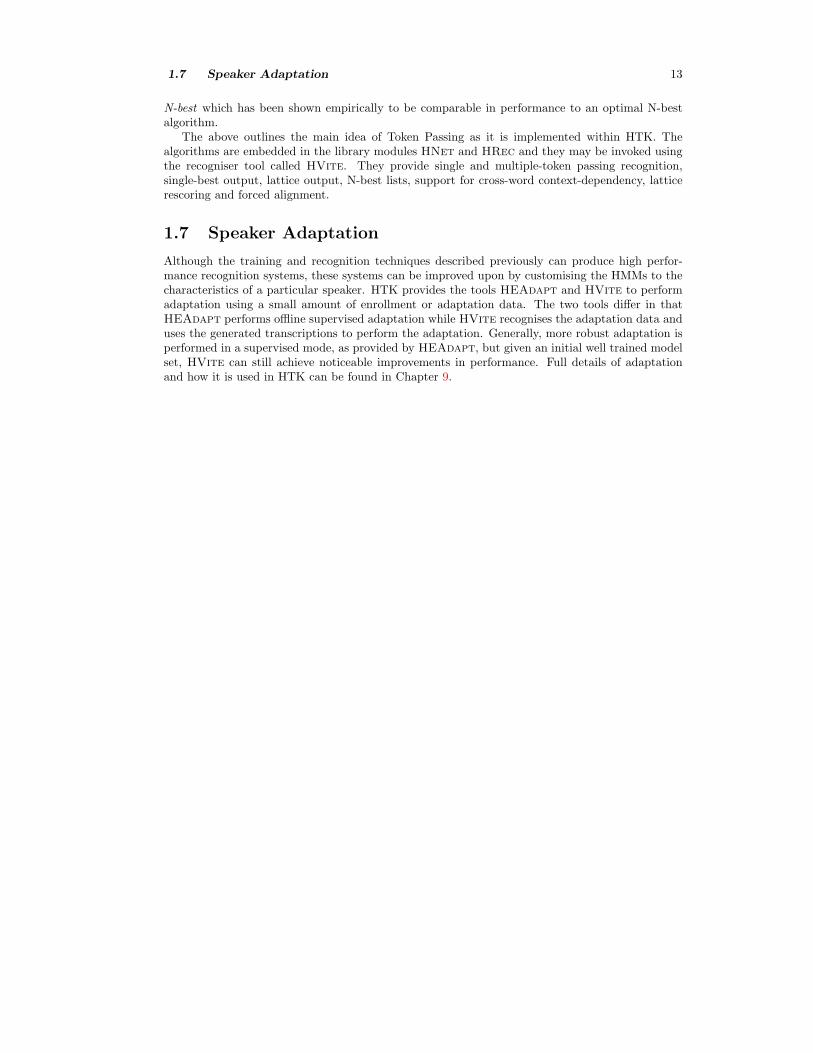
Although the training and recognition techniques described previously can produce high perfor-mance recognition systems, these systems can be improved upon by customising the HMMs to thecharacteristics of a particular speaker. HTK provides the tools HEAdapt and HVite to performadaptation using a small amount of enrollment or adaptation data. The two tools differ in thatHEAdapt performs offline supervised adaptation while HVite recognises the adaptation data anduses the generated transcriptions to perform the adaptation. Generally, more robust adaptation isperformed in a supervised mode, as provided by HEAdapt, but given an initial well trained modelset, HVite can still achieve noticeable improvements in performance. Full details of adaptationand how it is used in HTK can be found in Chapter 9.

Chapter 2

An Overview of the HTK Toolkit

Entr�opic

Darpa TIM IT

NIST

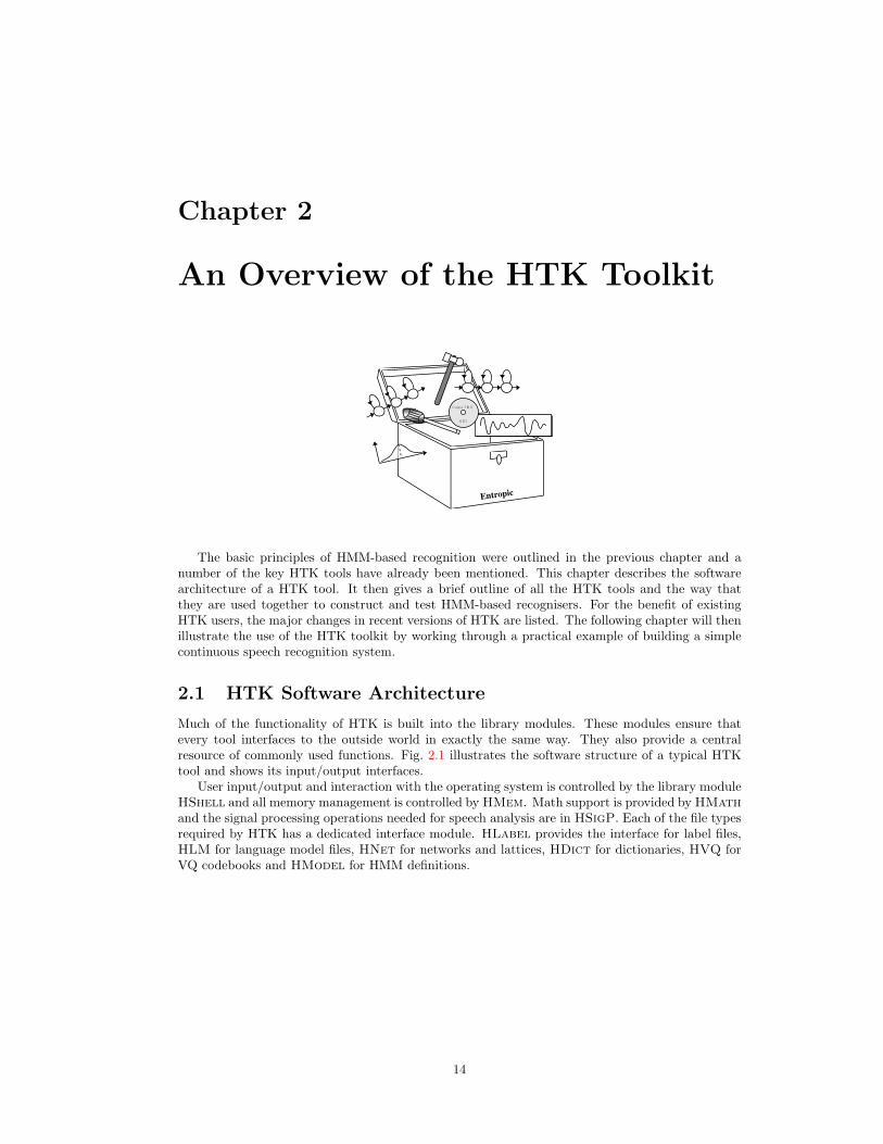
The basic principles of HMM-based recognition were outlined in the previous chapter and anumber of the key HTK tools have already been mentioned. This chapter describes the softwarearchitecture of a HTK tool. It then gives a brief outline of all the HTK tools and the way thatthey are used together to construct and test HMM-based recognisers. For the benefit of existingHTK users, the major changes in recent versions of HTK are listed. The following chapter will thenillustrate the use of the HTK toolkit by working through a practical example of building a simplecontinuous speech recognition system.

2.1 HTK Software Architecture

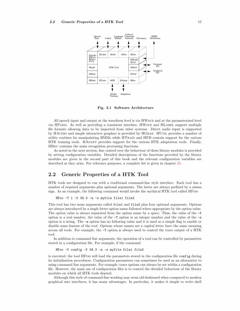
Much of the functionality of HTK is built into the library modules. These modules ensure thatevery tool interfaces to the outside world in exactly the same way. They also provide a centralresource of commonly used functions. Fig. 2.1 illustrates the software structure of a typical HTKtool and shows its input/output interfaces.

User input/output and interaction with the operating system is controlled by the library moduleHShell and all memory management is controlled by HMem. Math support is provided by HMath

and the signal processing operations needed for speech analysis are in HSigP. Each of the file typesrequired by HTK has a dedicated interface module. HLabel provides the interface for label files,HLM for language model files, HNet for networks and lattices, HDict for dictionaries, HVQ forVQ codebooks and HModel for HMM definitions.

14

2.2 Generic Properties of a HTK Tool 15

SpeechData Definitions

HMM

Terminal

Graphical

AdaptationModelTraining

HNet

LanguageModels

ConstraintNetwork

Lattices/

Dictionary

HModel

HDict

HUtil

HShell

HGraf

HRecHAdaptHMath

HMem

HSigP

HVQHParmHWaveHAudio

HTrain HFB

HTK Tool

I/O

I/O

HLM

Labels

HLabel

Fig. 2.1 Software Architecture

All speech input and output at the waveform level is via HWave and at the parameterised levelvia HParm. As well as providing a consistent interface, HWave and HLabel support multiplefile formats allowing data to be imported from other systems. Direct audio input is supportedby HAudio and simple interactive graphics is provided by HGraf. HUtil provides a number ofutility routines for manipulating HMMs while HTrain and HFB contain support for the variousHTK training tools. HAdapt provides support for the various HTK adaptation tools. Finally,HRec contains the main recognition processing functions.

As noted in the next section, fine control over the behaviour of these library modules is providedby setting configuration variables. Detailed descriptions of the functions provided by the librarymodules are given in the second part of this book and the relevant configuration variables aredescribed as they arise. For reference purposes, a complete list is given in chapter 15.

2.2 Generic Properties of a HTK Tool

HTK tools are designed to run with a traditional command-line style interface. Each tool has anumber of required arguments plus optional arguments. The latter are always prefixed by a minussign. As an example, the following command would invoke the mythical HTK tool called HFoo

HFoo -T 1 -f 34.3 -a -s myfile file1 file2

This tool has two main arguments called file1 and file2 plus four optional arguments. Optionsare always introduced by a single letter option name followed where appropriate by the option value.The option value is always separated from the option name by a space. Thus, the value of the -f

option is a real number, the value of the -T option is an integer number and the value of the -s

option is a string. The -a option has no following value and it is used as a simple flag to enable ordisable some feature of the tool. Options whose names are a capital letter have the same meaningacross all tools. For example, the -T option is always used to control the trace output of a HTKtool.

In addition to command line arguments, the operation of a tool can be controlled by parametersstored in a configuration file. For example, if the command

HFoo -C config -f 34.3 -a -s myfile file1 file2

is executed, the tool HFoo will load the parameters stored in the configuration file config duringits initialisation procedures. Configuration parameters can sometimes be used as an alternative tousing command line arguments. For example, trace options can always be set within a configurationfile. However, the main use of configuration files is to control the detailed behaviour of the librarymodules on which all HTK tools depend.

Although this style of command-line working may seem old-fashioned when compared to moderngraphical user interfaces, it has many advantages. In particular, it makes it simple to write shell

2.3 The Toolkit 16

scripts to control HTK tool execution. This is vital for performing large-scale system buildingand experimentation. Furthermore, defining all operations using text-based commands allows thedetails of system construction or experimental procedure to be recorded and documented.

Finally, note that a summary of the command line and options for any HTK tool can be obtainedsimply by executing the tool with no arguments.

2.3 The Toolkit

The HTK tools are best introduced by going through the processing steps involved in building asub-word based continuous speech recogniser. As shown in Fig. 2.2, there are 4 main phases: datapreparation, training, testing and analysis.

2.3.1 Data Preparation Tools

In order to build a set of HMMs, a set of speech data files and their associated transcriptions arerequired. Very often speech data will be obtained from database archives, typically on CD-ROMs.Before it can be used in training, it must be converted into the appropriate parametric form andany associated transcriptions must be converted to have the correct format and use the requiredphone or word labels. If the speech needs to be recorded, then the tool HSLab can be used bothto record the speech and to manually annotate it with any required transcriptions.

Although all HTK tools can parameterise waveforms on-the-fly, in practice it is usually better toparameterise the data just once. The tool HCopy is used for this. As the name suggests, HCopy

is used to copy one or more source files to an output file. Normally, HCopy copies the whole file,but a variety of mechanisms are provided for extracting segments of files and concatenating files.By setting the appropriate configuration variables, all input files can be converted to parametricform as they are read-in. Thus, simply copying each file in this manner performs the requiredencoding. The tool HList can be used to check the contents of any speech file and since it can alsoconvert input on-the-fly, it can be used to check the results of any conversions before processinglarge quantities of data. Transcriptions will also need preparing. Typically the labels used in theoriginal source transcriptions will not be exactly as required, for example, because of differences inthe phone sets used. Also, HMM training might require the labels to be context-dependent. Thetool HLEd is a script-driven label editor which is designed to make the required transformationsto label files. HLEd can also output files to a single Master Label File MLF which is usuallymore convenient for subsequent processing. Finally on data preparation, HLStats can gather anddisplay statistics on label files and where required, HQuant can be used to build a VQ codebookin preparation for building discrete probability HMM system.

2.3.2 Training Tools

The second step of system building is to define the topology required for each HMM by writing aprototype definition. HTK allows HMMs to be built with any desired topology. HMM definitionscan be stored externally as simple text files and hence it is possible to edit them with any convenienttext editor. Alternatively, the standard HTK distribution includes a number of example HMMprototypes and a script to generate the most common topologies automatically. With the exceptionof the transition probabilities, all of the HMM parameters given in the prototype definition areignored. The purpose of the prototype definition is only to specify the overall characteristics andtopology of the HMM. The actual parameters will be computed later by the training tools. Sensiblevalues for the transition probabilities must be given but the training process is very insensitiveto these. An acceptable and simple strategy for choosing these probabilities is to make all of thetransitions out of any state equally likely.

2.3 The Toolkit 17

HPARSE

HVITE

HCOMPV, HINIT , HREST , HEREST

DataPrep

Training

Testing

Analysis

HMMs

Networks

Dictionary

HLE

HDMAN

HQ

HSLAB

HCHL

Speech

D

HLS

UANT

IST

OPYTATS

HR

HBUILD

ESULTS

HSMOOTH, HHED DAPT, HEA

Transcriptions

Transcriptions

Fig. 2.2 HTK Processing Stages

The actual training process takes place in stages and it is illustrated in more detail in Fig. 2.3.Firstly, an initial set of models must be created. If there is some speech data available for whichthe location of the sub-word (i.e. phone) boundaries have been marked, then this can be used asbootstrap data. In this case, the tools HInit and HRest provide isolated word style training usingthe fully labelled bootstrap data. Each of the required HMMs is generated individually. HInit

reads in all of the bootstrap training data and cuts out all of the examples of the required phone. Itthen iteratively computes an initial set of parameter values using a segmental k-means procedure.On the first cycle, the training data is uniformly segmented, each model state is matched with thecorresponding data segments and then means and variances are estimated. If mixture Gaussianmodels are being trained, then a modified form of k-means clustering is used. On the secondand successive cycles, the uniform segmentation is replaced by Viterbi alignment. The initialparameter values computed by HInit are then further re-estimated by HRest. Again, the fullylabelled bootstrap data is used but this time the segmental k-means procedure is replaced by theBaum-Welch re-estimation procedure described in the previous chapter. When no bootstrap datais available, a so-called flat start can be used. In this case all of the phone models are initialisedto be identical and have state means and variances equal to the global speech mean and variance.The tool HCompV can be used for this.

2.3 The Toolkit 18

HCompV

HERest

HHEd

th ih s ih s p iy t sh

sh t iy s z�

ih s ih th

Labelled Utterances

HRest

HInit

Sub-WordHMMs

Unlabelled Utterances

Transcriptions

th ih s ih s p iy t sh

sh t iy s z�

ih s ih th

Fig. 2.3 Training Sub-word HMMs

Once an initial set of models has been created, the tool HERest is used to perform embedded

training using the entire training set. HERest performs a single Baum-Welch re-estimation of thewhole set of HMM phone models simultaneously. For each training utterance, the correspondingphone models are concatenated and then the forward-backward algorithm is used to accumulate thestatistics of state occupation, means, variances, etc., for each HMM in the sequence. When all ofthe training data has been processed, the accumulated statistics are used to compute re-estimatesof the HMM parameters. HERest is the core HTK training tool. It is designed to process largedatabases, it has facilities for pruning to reduce computation and it can be run in parallel across anetwork of machines.

The philosophy of system construction in HTK is that HMMs should be refined incrementally.Thus, a typical progression is to start with a simple set of single Gaussian context-independentphone models and then iteratively refine them by expanding them to include context-dependencyand use multiple mixture component Gaussian distributions. The tool HHEd is a HMM definitioneditor which will clone models into context-dependent sets, apply a variety of parameter tyingsand increment the number of mixture components in specified distributions. The usual processis to modify a set of HMMs in stages using HHEd and then re-estimate the parameters of themodified set using HERest after each stage. To improve performance for specific speakers thetools HEAdapt and HVite can be used to adapt HMMs to better model the characteristics ofparticular speakers using a small amount of training or adaptation data. The end result of whichis a speaker adapted system.

The single biggest problem in building context-dependent HMM systems is always data insuffi-ciency. The more complex the model set, the more data is needed to make robust estimates of itsparameters, and since data is usually limited, a balance must be struck between complexity andthe available data. For continuous density systems, this balance is achieved by tying parameterstogether as mentioned above. Parameter tying allows data to be pooled so that the shared param-eters can be robustly estimated. In addition to continuous density systems, HTK also supports

2.4 Whats New In Version 2.2 19

fully tied mixture systems and discrete probability systems. In these cases, the data insufficiencyproblem is usually addressed by smoothing the distributions and the tool HSmooth is used forthis.

2.3.3 Recognition Tools

HTK provides a single recognition tool called HVite which uses the token passing algorithm de-scribed in the previous chapter to perform Viterbi-based speech recognition. HVite takes as inputa network describing the allowable word sequences, a dictionary defining how each word is pro-nounced and a set of HMMs. It operates by converting the word network to a phone network andthen attaching the appropriate HMM definition to each phone instance. Recognition can then beperformed on either a list of stored speech files or on direct audio input. As noted at the end ofthe last chapter, HVite can support cross-word triphones and it can run with multiple tokens togenerate lattices containing multiple hypotheses. It can also be configured to rescore lattices andperform forced alignments.

The word networks needed to drive HVite are usually either simple word loops in which anyword can follow any other word or they are directed graphs representing a finite-state task grammar.In the former case, bigram probabilities are normally attached to the word transitions. Wordnetworks are stored using the HTK standard lattice format. This is a text-based format and henceword networks can be created directly using a text-editor. However, this is rather tedious and henceHTK provides two tools to assist in creating word networks. Firstly, HBuild allows sub-networksto be created and used within higher level networks. Hence, although the same low level notation isused, much duplication is avoided. Also, HBuild can be used to generate word loops and it can alsoread in a backed-off bigram language model and modify the word loop transitions to incorporatethe bigram probabilities. Note that the label statistics tool HLStats mentioned earlier can be usedto generate a backed-off bigram language model.

As an alternative to specifying a word network directly, a higher level grammar notation canbe used. This notation is based on the Extended Backus Naur Form (EBNF) used in compilerspecification and it is compatible with the grammar specification language used in earlier versionsof HTK. The tool HParse is supplied to convert this notation into the equivalent word network.

Whichever method is chosen to generate a word network, it is useful to be able to see examplesof the language that it defines. The tool HSGen is provided to do this. It takes as input anetwork and then randomly traverses the network outputting word strings. These strings can thenbe inspected to ensure that they correspond to what is required. HSGen can also compute theempirical perplexity of the task.

Finally, the construction of large dictionaries can involve merging several sources and performinga variety of transformations on each sources. The dictionary management tool HDMan is suppliedto assist with this process.

2.3.4 Analysis Tool

Once the HMM-based recogniser has been built, it is necessary to evaluate its performance. Thisis usually done by using it to transcribe some pre-recorded test sentences and match the recogniseroutput with the correct reference transcriptions. This comparison is performed by a tool calledHResults which uses dynamic programming to align the two transcriptions and then count sub-stitution, deletion and insertion errors. Options are provided to ensure that the algorithms andoutput formats used by HResults are compatible with those used by the US National Instituteof Standards and Technology (NIST). As well as global performance measures, HResults canalso provide speaker-by-speaker breakdowns, confusion matrices and time-aligned transcriptions.For word spotting applications, it can also compute Figure of Merit (FOM) scores and Receiver

Operating Curve (ROC) information.

2.4 Whats New In Version 2.2

This section lists the new features and refinements in HTK Version 2.2 compared to the precedingVersion 2.1.

1. Speaker adaptation is now supported via the HEAdapt and HVite tools, which adapt acurrent set of models to a new speaker and/or environment.

2.4 Whats New In Version 2.2 20

• HEAdapt performs offline supervised adaptation using maximum likelihood linear re-gression (MLLR) and/or maximum a-posteriori (MAP) adaptation.

• HVite performs unsupervised adaptation using just MLLR.

Both tools can be used in a static mode, where all the data is presented prior to any adaptation,or in an incremental fashion.

2. Improved support for PC WAV filesIn addition to 16-bit PCM linear, HTK can now read

• 8-bit CCITT mu-law

• 8-bit CCITT a-law

• 8-bit PCM linear

2.4.1 Features Added To Version 2.1

For the benefit of users of earlier versions of HTK this section lists the main changes in HTKVersion 2.1 compared to the preceding Version 2.0.

1. The speech input handling has been partially re-designed and a new energy-based speech/silencedetector has been incorporated into HParm. The detector is robust yet flexible and can beconfigured through a number of configuration variables. Speech/silence detection can now beperformed on waveform files. The calibration of speech/silence detector parameters is nowaccomplished by asking the user to speak an arbitrary sentence.

2. HParm now allows random noise signal to be added to waveform data via the configurationparameter ADDDITHER. This prevents numerical overflows which can occur with artificiallycreated waveform data under some coding schemes.

3. HNet has been optimised for more efficient operation when performing forced alignments ofutterances using HVite. Further network optimisations tailored to biphone/triphone-basedphone recognition have also been incorporated.

4. HVite can now produce partial recognition hypothesis even when no tokens survive to the endof the network. This is accomplished by setting the HRec configuration parameter FORCEOUTto true.

5. Dictionary support has been extended to allow pronunciation probabilities to be associatedwith different pronunciations of the same word. At the same time, HVite now allows the useof a pronunciation scale factor during recognition.

6. HTK now provides consistent support for reading and writing of HTK binary files (waveforms,binary MMFs, binary SLFs, HERest accumulators) across different machine architecturesincorporating automatic byte swapping. By default, all binary data files handled by the toolsare now written/read in big-endian (NONVAX) byte order. The default behavior can be changedvia the configuration parameters NATURALREADORDER and NATURALWRITEORDER.

7. HWave supports the reading of waveforms in Microsoft WAVE file format.

8. HAudio allows key-press control of live audio input.

Chapter 3

A Tutorial Example of Using HTK

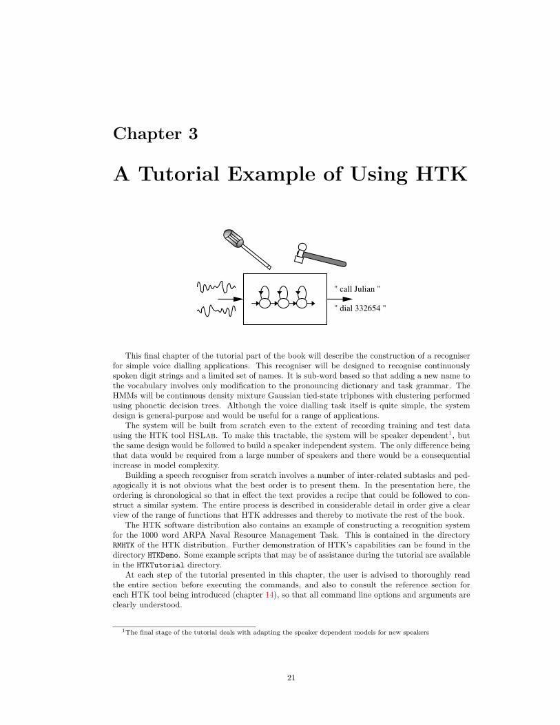
" call Julian "

" dial 332654 "

This final chapter of the tutorial part of the book will describe the construction of a recogniserfor simple voice dialling applications. This recogniser will be designed to recognise continuouslyspoken digit strings and a limited set of names. It is sub-word based so that adding a new name tothe vocabulary involves only modification to the pronouncing dictionary and task grammar. TheHMMs will be continuous density mixture Gaussian tied-state triphones with clustering performedusing phonetic decision trees. Although the voice dialling task itself is quite simple, the systemdesign is general-purpose and would be useful for a range of applications.

The system will be built from scratch even to the extent of recording training and test datausing the HTK tool HSLab. To make this tractable, the system will be speaker dependent1, butthe same design would be followed to build a speaker independent system. The only difference beingthat data would be required from a large number of speakers and there would be a consequentialincrease in model complexity.

Building a speech recogniser from scratch involves a number of inter-related subtasks and ped-agogically it is not obvious what the best order is to present them. In the presentation here, theordering is chronological so that in effect the text provides a recipe that could be followed to con-struct a similar system. The entire process is described in considerable detail in order give a clearview of the range of functions that HTK addresses and thereby to motivate the rest of the book.

The HTK software distribution also contains an example of constructing a recognition systemfor the 1000 word ARPA Naval Resource Management Task. This is contained in the directoryRMHTK of the HTK distribution. Further demonstration of HTK’s capabilities can be found in thedirectory HTKDemo. Some example scripts that may be of assistance during the tutorial are availablein the HTKTutorial directory.

At each step of the tutorial presented in this chapter, the user is advised to thoroughly readthe entire section before executing the commands, and also to consult the reference section foreach HTK tool being introduced (chapter 14), so that all command line options and arguments areclearly understood.

1The final stage of the tutorial deals with adapting the speaker dependent models for new speakers

21

3.1 Data Preparation 22

3.1 Data Preparation

The first stage of any recogniser development project is data preparation. Speech data is neededboth for training and for testing. In the system to be built here, all of this speech will be recordedfrom scratch and to do this scripts are needed to prompt for each sentence. In the case of thetest data, these prompt scripts will also provide the reference transcriptions against which therecogniser’s performance can be measured and a convenient way to create them is to use the taskgrammar as a random generator. In the case of the training data, the prompt scripts will be used inconjunction with a pronunciation dictionary to provide the initial phone level transcriptions neededto start the HMM training process. Since the application requires that arbitrary names can beadded to the recogniser, training data with good phonetic balance and coverage is needed. Herefor convenience the prompt scripts needed for training are taken from the TIMIT acoustic-phoneticdatabase.

It follows from the above that before the data can be recorded, a phone set must be defined,a dictionary must be constructed to cover both training and testing and a task grammar must bedefined.

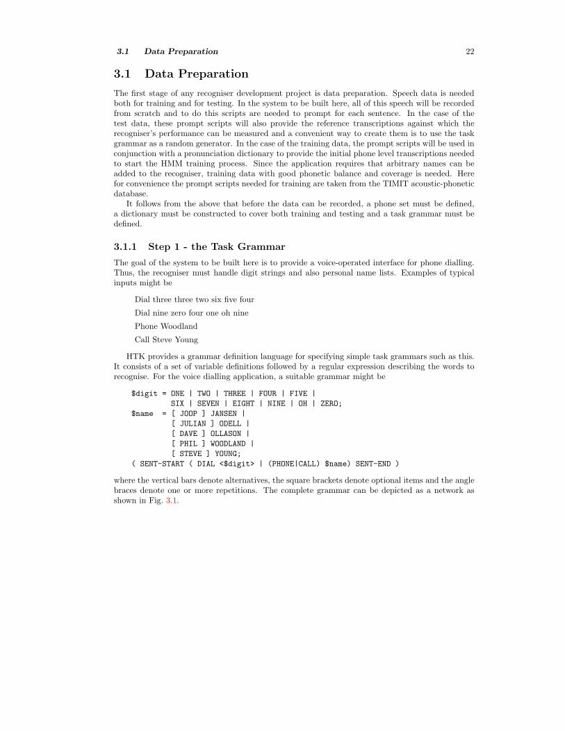
3.1.1 Step 1 - the Task Grammar

The goal of the system to be built here is to provide a voice-operated interface for phone dialling.Thus, the recogniser must handle digit strings and also personal name lists. Examples of typicalinputs might be

Dial three three two six five four

Dial nine zero four one oh nine

Phone Woodland

Call Steve Young

HTK provides a grammar definition language for specifying simple task grammars such as this.It consists of a set of variable definitions followed by a regular expression describing the words torecognise. For the voice dialling application, a suitable grammar might be

$digit = ONE | TWO | THREE | FOUR | FIVE |

SIX | SEVEN | EIGHT | NINE | OH | ZERO;

$name = [ JOOP ] JANSEN |

[ JULIAN ] ODELL |

[ DAVE ] OLLASON |

[ PHIL ] WOODLAND |

[ STEVE ] YOUNG;

( SENT-START ( DIAL <$digit> | (PHONE|CALL) $name) SENT-END )

where the vertical bars denote alternatives, the square brackets denote optional items and the anglebraces denote one or more repetitions. The complete grammar can be depicted as a network asshown in Fig. 3.1.


sent-start

one

two

three

zero

dial

phone

call

Julian Odell

Dave

... etc

Steve Young

... etc

Ollason

sent-end

Fig. 3.1 Grammar for Voice Dialling

Grammar

(gram)

Word Net

(wdnet)

HPA�

RSE

Fig. 3.2Step 1

The above high level representation of a task grammar is provided for user convenience. TheHTK recogniser actually requires a word network to be defined using a low level notation calledHTK Standard Lattice Format (SLF) in which each word instance and each word-to-word transitionis listed explicitly. This word network can be created automatically from the grammar above usingthe HParse tool, thus assuming that the file gram contains the above grammar, executing

HParse gram wdnet

will create an equivalent word network in the file wdnet (see Fig 3.2).

3.1.2 Step 2 - the Dictionary

The first step in building a dictionary is to create a sorted list of the required words. In the telephonedialling task pursued here, it is quite easy to create a list of required words by hand. However, ifthe task were more complex, it would be necessary to build a word list from the sample sentencespresent in the training data. Furthermore, to build robust acoustic models, it is necessary to trainthem on a large set of sentences containing many words and preferably phonetically balanced. Forthese reasons, the training data will consist of English sentences unrelated to the phone recognitiontask. Below, a short example of creating a word list from sentence prompts will be given. As notedabove the training sentences given here are extracted from some prompts used with the TIMITdatabase and for convenience reasons they have been renumbered. For example, the first few itemsmight be as follows


S0001 ONE VALIDATED ACTS OF SCHOOL DISTRICTS

S0002 TWO OTHER CASES ALSO WERE UNDER ADVISEMENT

S0003 BOTH FIGURES WOULD GO HIGHER IN LATER YEARS

S0004 THIS IS NOT A PROGRAM OF SOCIALIZED MEDICINE

etc

The desired training word list (wlist) could then be extracted automatically from these. Beforeusing HTK, one would need to edit the text into a suitable format. For example, it would benecessary to change all white space to newlines and then to use the UNIX utilities sort and uniq

to sort the words into a unique alphabetically ordered set, with one word per line. The scriptprompts2wlist from the HTKTutorial directory can be used for this purpose.

The dictionary itself can be built from a standard source using HDMan. For this example, theBritish English BEEP pronouncing dictionary will be used2. Its phone set will be adopted withoutmodification except that the stress marks will be removed and a short-pause (sp) will be added tothe end of every pronunciation. If the dictionary contains any silence markers then the MP commandwill merge the sil and sp phones into a single sil. These changes can be applied using HDMan

and an edit script (stored in global.ded) containing the three commands

AS sp

RS cmu

MP sil sil sp

where cmu refers to a style of stress marking in which the lexical stress level is marked by a singledigit appended to the phone name (e.g. eh2 means the phone eh with level 2 stress).

TIMITPrompts

Word List(wlist)

sort | uniq

Edit Script(global.ded)

HDM�

AN

BEEP Dict(beep)

Names Dict(names)

Dictionary(dict)

+

TestVocab

Fig. 3.3 Step 2

The command

HDMan -m -w wlist -n monophones1 -l dlog dict beep names

will create a new dictionary called dict by searching the source dictionaries beep and names to findpronunciations for each word in wlist (see Fig 3.3). Here, the wlist in question needs only to bea sorted list of the words appearing in the task grammar given above.

Note that names is a manually constructed file containing pronunciations for the proper namesused in the task grammar. The option -l instructs HDMan to output a log file dlog whichcontains various statistics about the constructed dictionary. In particular, it indicates if there arewords missing. HDMan can also output a list of the phones used, here called monophones1. Oncetraining and test data has been recorded, an HMM will be estimated for each of these phones.

The general format of each dictionary entry is

WORD [outsym] p1 p2 p3 ....

2Available by anonymous ftp from svr-ftp.eng.cam.ac.uk/pub/comp.speech/dictionaries/beep.tar.gz. Notethat items beginning with unmatched quotes, found at the start of the dictionary, should be removed.


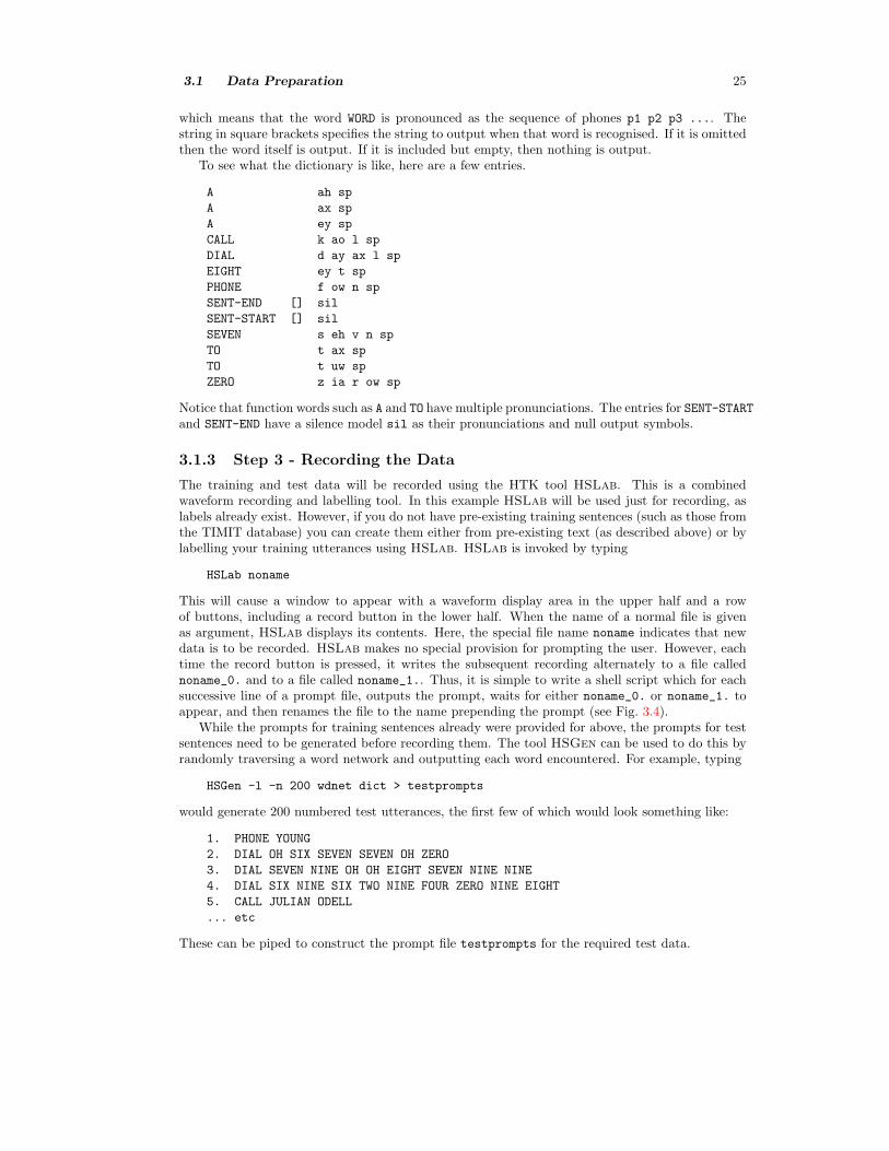
which means that the word WORD is pronounced as the sequence of phones p1 p2 p3 .... Thestring in square brackets specifies the string to output when that word is recognised. If it is omittedthen the word itself is output. If it is included but empty, then nothing is output.

To see what the dictionary is like, here are a few entries.

A ah sp

A ax sp

A ey sp

CALL k ao l sp

DIAL d ay ax l sp

EIGHT ey t sp

PHONE f ow n sp

SENT-END [] sil

SENT-START [] sil

SEVEN s eh v n sp

TO t ax sp

TO t uw sp

ZERO z ia r ow sp

Notice that function words such as A and TO have multiple pronunciations. The entries for SENT-STARTand SENT-END have a silence model sil as their pronunciations and null output symbols.

3.1.3 Step 3 - Recording the Data

The training and test data will be recorded using the HTK tool HSLab. This is a combinedwaveform recording and labelling tool. In this example HSLab will be used just for recording, aslabels already exist. However, if you do not have pre-existing training sentences (such as those fromthe TIMIT database) you can create them either from pre-existing text (as described above) or bylabelling your training utterances using HSLab. HSLab is invoked by typing

HSLab noname

This will cause a window to appear with a waveform display area in the upper half and a rowof buttons, including a record button in the lower half. When the name of a normal file is givenas argument, HSLab displays its contents. Here, the special file name noname indicates that newdata is to be recorded. HSLab makes no special provision for prompting the user. However, eachtime the record button is pressed, it writes the subsequent recording alternately to a file callednoname_0. and to a file called noname_1.. Thus, it is simple to write a shell script which for eachsuccessive line of a prompt file, outputs the prompt, waits for either noname_0. or noname_1. toappear, and then renames the file to the name prepending the prompt (see Fig. 3.4).

While the prompts for training sentences already were provided for above, the prompts for testsentences need to be generated before recording them. The tool HSGen can be used to do this byrandomly traversing a word network and outputting each word encountered. For example, typing

HSGen -l -n 200 wdnet dict > testprompts

would generate 200 numbered test utterances, the first few of which would look something like:

1. PHONE YOUNG

2. DIAL OH SIX SEVEN SEVEN OH ZERO

3. DIAL SEVEN NINE OH OH EIGHT SEVEN NINE NINE

4. DIAL SIX NINE SIX TWO NINE FOUR ZERO NINE EIGHT

5. CALL JULIAN ODELL

... etc

These can be piped to construct the prompt file testprompts for the required test data.


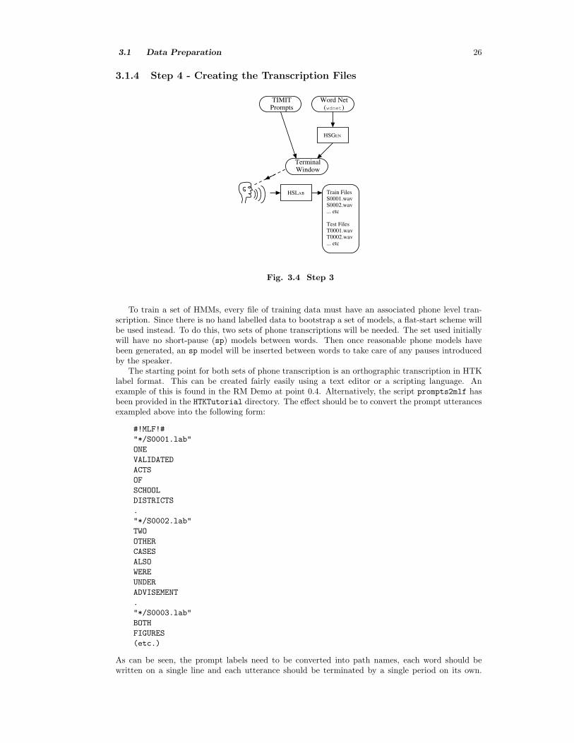
3.1.4 Step 4 - Creating the Transcription Files

TIMITPrompts

TerminalWindow

HSG�

EN

Word Net(wdnet)

HSL�

AB Train FilesS0001.wavS0002.wav... etc

Test FilesT0001.wavT0002.wav... etc

Fig. 3.4 Step 3

To train a set of HMMs, every file of training data must have an associated phone level tran-scription. Since there is no hand labelled data to bootstrap a set of models, a flat-start scheme willbe used instead. To do this, two sets of phone transcriptions will be needed. The set used initiallywill have no short-pause (sp) models between words. Then once reasonable phone models havebeen generated, an sp model will be inserted between words to take care of any pauses introducedby the speaker.

The starting point for both sets of phone transcription is an orthographic transcription in HTKlabel format. This can be created fairly easily using a text editor or a scripting language. Anexample of this is found in the RM Demo at point 0.4. Alternatively, the script prompts2mlf hasbeen provided in the HTKTutorial directory. The effect should be to convert the prompt utterancesexampled above into the following form:

#!MLF!#

"*/S0001.lab"

ONE

VALIDATED

ACTS

OF

SCHOOL

DISTRICTS

.

"*/S0002.lab"

TWO

OTHER

CASES

ALSO

WERE

UNDER

ADVISEMENT

.

"*/S0003.lab"

BOTH

FIGURES

(etc.)

As can be seen, the prompt labels need to be converted into path names, each word should bewritten on a single line and each utterance should be terminated by a single period on its own.


The first line of the file just identifies the file as a Master Label File (MLF). This is a single filecontaining a complete set of transcriptions. HTK allows each individual transcription to be storedin its own file but it is more efficient to use an MLF.

The form of the path name used in the MLF deserves some explanation since it is really a pattern

and not a name. When HTK processes speech files, it expects to find a transcription (or label file)with the same name but a different extension. Thus, if the file /root/sjy/data/S0001.wav wasbeing processed, HTK would look for a label file called /root/sjy/data/S0001.lab. When MLFfiles are used, HTK scans the file for a pattern which matches the required label file name. However,an asterix will match any character string and hence the pattern used in the example is in effectpath independent. It therefore allows the same transcriptions to be used with different versions ofthe speech data to be stored in different locations.

Once the word level MLF has been created, phone level MLFs can be generated using the labeleditor HLEd. For example, assuming that the above word level MLF is stored in the file words.mlf,the command

HLEd -l ’*’ -d dict -i phones0.mlf mkphones0.led words.mlf

will generate a phone level transcription of the following form where the -l option is needed togenerate the path ’*’ in the output patterns.

#!MLF!#

"*/S0001.lab"

sil

w

ah

n

v

ae

l

ih

d

.. etc

This process is illustrated in Fig. 3.5.The HLEd edit script mkphones0.led contains the following commands

EX

IS sil sil

DE sp

The expand EX command replaces each word in words.mlf by the corresponding pronunciation inthe dictionary file dict. The IS command inserts a silence model sil at the start and end of everyutterance. Finally, the delete DE command deletes all short-pause sp labels, which are not wantedin the transcription labels at this point.


TIMITPrompts

Edit Script(mkphones0.led)

HL�

ED

Phone LevelTranscription(phones0.mlf)

Dictionary(dict)

Word LevelTranscription(words.mlf)

Fig. 3.5 Step 4

3.1.5 Step 5 - Coding the Data

The final stage of data preparation is to parameterise the raw speech waveforms into sequencesof feature vectors. HTK support both FFT-based and LPC-based analysis. Here Mel FrequencyCepstral Coefficients (MFCCs), which are derived from FFT-based log spectra, will be used.

Coding can be performed using the tool HCopy configured to automatically convert its inputinto MFCC vectors. To do this, a configuration file (config) is needed which specifies all of theconversion parameters. Reasonable settings for these are as follows

# Coding parameters

TARGETKIND = MFCC_0

TARGETRATE = 100000.0

SAVECOMPRESSED = T

SAVEWITHCRC = T

WINDOWSIZE = 250000.0

USEHAMMING = T

PREEMCOEF = 0.97

NUMCHANS = 26

CEPLIFTER = 22

NUMCEPS = 12

ENORMALISE = F

Some of these settings are in fact the default setting, but they are given explicitly here for com-pleteness. In brief, they specify that the target parameters are to be MFCC using C0 as the energycomponent, the frame period is 10msec (HTK uses units of 100ns), the output should be saved incompressed format, and a crc checksum should be added. The FFT should use a Hamming windowand the signal should have first order preemphasis applied using a coefficient of 0.97. The filterbankshould have 26 channels and 12 MFCC coefficients should be output. The variable ENORMALISE isby default true and performs energy normalisation on recorded audio files. It cannot be used withlive audio and since the target system is for live audio, this variable should be set to false.

Note that explicitly creating coded data files is not necessary, as coding can be done ”on-the-fly”from the original waveform files by specifying the appropriate configuration file (as above) with therelevant HTK tools. However, creating these files reduces the amount of preprocessing requiredduring training, which itself can be a time-consuming process.

To run HCopy, a list of each source file and its corresponding output file is needed. For example,the first few lines might look like

3.2 Creating Monophone HMMs 29

/root/sjy/waves/S0001.wav /root/sjy/train/S0001.mfc




(etc.)

Files containing lists of files are referred to as script files3 and by convention are given the extensionscp (although HTK does not demand this). Script files are specified using the standard -S optionand their contents are read simply as extensions to the command line. Thus, they avoid the needfor command lines with several thousand arguments4.

ConfigurationFile

(config)

Script File(codetr.scp)

HCOPY

Waveform FilesS0001.wav

S0002.wav

S0003.wav

etc

MFCC FilesS0001.mfc

S0002.mfc

S0003.mfc

etc

Fig. 3.6 Step 5

Assuming that the above script is stored in the file codetr.scp, the training data would be codedby executing

HCopy -T 1 -C config -S codetr.scp

This is illustrated in Fig. 3.6. A similar procedure is used to code the test data (using TARGETKIND = MFCC_0_D_A

in config) after which all of the pieces are in place to start training the HMMs.

3.2 Creating Monophone HMMs

In this section, the creation of a well-trained set of single-Gaussian monophone HMMs will bedescribed. The starting point will be a set of identical monophone HMMs in which every mean andvariance is identical. These are then retrained, short-pause models are added and the silence modelis extended slightly. The monophones are then retrained.

Some of the dictionary entries have multiple pronunciations. However, when HLEd was usedto expand the word level MLF to create the phone level MLFs, it arbitrarily selected the firstpronunciation it found. Once reasonable monophone HMMs have been created, the recogniser toolHVite can be used to perform a forced alignment of the training data. By this means, a new phonelevel MLF is created in which the choice of pronunciations depends on the acoustic evidence. Thisnew MLF can be used to perform a final re-estimation of the monophone HMMs.

3.2.1 Step 6 - Creating Flat Start Monophones

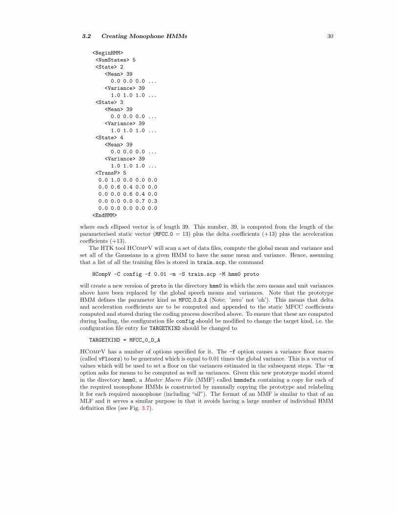
The first step in HMM training is to define a prototype model. The parameters of this modelare not important, its purpose is to define the model topology. For phone-based systems, a goodtopology to use is 3-state left-right with no skips such as the following

~o <VecSize> 39 <MFCC_0_D_A>

~h "proto"

3 Not to be confused with files containing edit scripts4 Most UNIX shells, especially the C shell, only allow a limited and quite small number of arguments.


<BeginHMM>

<NumStates> 5

<State> 2

<Mean> 39

0.0 0.0 0.0 ...

<Variance> 39

1.0 1.0 1.0 ...

<State> 3

<Mean> 39

0.0 0.0 0.0 ...

<Variance> 39

1.0 1.0 1.0 ...

<State> 4

<Mean> 39

0.0 0.0 0.0 ...

<Variance> 39

1.0 1.0 1.0 ...

<TransP> 5

0.0 1.0 0.0 0.0 0.0

0.0 0.6 0.4 0.0 0.0

0.0 0.0 0.6 0.4 0.0

0.0 0.0 0.0 0.7 0.3

0.0 0.0 0.0 0.0 0.0

<EndHMM>

where each ellipsed vector is of length 39. This number, 39, is computed from the length of theparameterised static vector (MFCC 0 = 13) plus the delta coefficients (+13) plus the accelerationcoefficients (+13).

The HTK tool HCompV will scan a set of data files, compute the global mean and variance andset all of the Gaussians in a given HMM to have the same mean and variance. Hence, assumingthat a list of all the training files is stored in train.scp, the command

HCompV -C config -f 0.01 -m -S train.scp -M hmm0 proto

will create a new version of proto in the directory hmm0 in which the zero means and unit variancesabove have been replaced by the global speech means and variances. Note that the prototypeHMM defines the parameter kind as MFCC 0 D A (Note: ’zero’ not ’oh’). This means that deltaand acceleration coefficients are to be computed and appended to the static MFCC coefficientscomputed and stored during the coding process described above. To ensure that these are computedduring loading, the configuration file config should be modified to change the target kind, i.e. theconfiguration file entry for TARGETKIND should be changed to

TARGETKIND = MFCC_0_D_A

HCompV has a number of options specified for it. The -f option causes a variance floor macro(called vFloors) to be generated which is equal to 0.01 times the global variance. This is a vector ofvalues which will be used to set a floor on the variances estimated in the subsequent steps. The -m

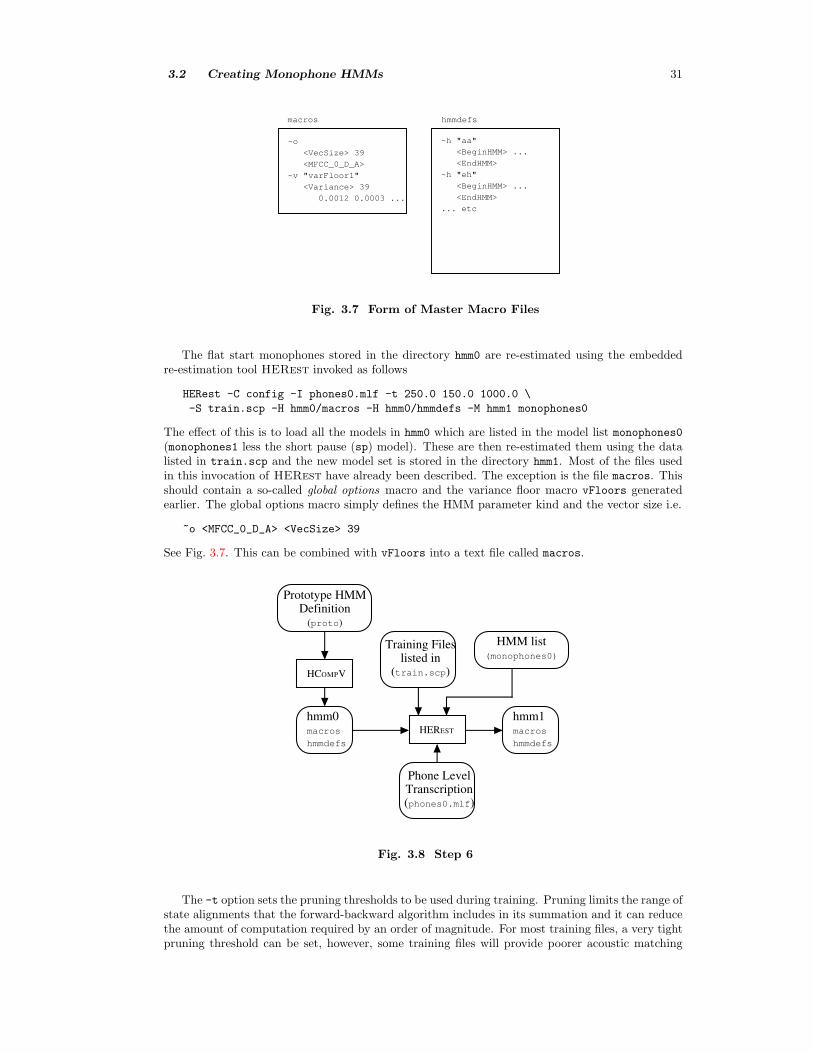
option asks for means to be computed as well as variances. Given this new prototype model storedin the directory hmm0, a Master Macro File (MMF) called hmmdefs containing a copy for each ofthe required monophone HMMs is constructed by manually copying the prototype and relabelingit for each required monophone (including “sil”). The format of an MMF is similar to that of anMLF and it serves a similar purpose in that it avoids having a large number of individual HMMdefinition files (see Fig. 3.7).


macros

~o

<VecSize> 39

<MFCC_0_D_A>

~v "varFloor1"

<Variance> 39

0.0012 0.0003 ...

hmmdefs

~h "aa"

<BeginHMM> ...

<EndHMM>

~h "eh"

<BeginHMM> ...

<EndHMM>

... etc

Fig. 3.7 Form of Master Macro Files

The flat start monophones stored in the directory hmm0 are re-estimated using the embeddedre-estimation tool HERest invoked as follows

HERest -C config -I phones0.mlf -t 250.0 150.0 1000.0 \

-S train.scp -H hmm0/macros -H hmm0/hmmdefs -M hmm1 monophones0

The effect of this is to load all the models in hmm0 which are listed in the model list monophones0(monophones1 less the short pause (sp) model). These are then re-estimated them using the datalisted in train.scp and the new model set is stored in the directory hmm1. Most of the files usedin this invocation of HERest have already been described. The exception is the file macros. Thisshould contain a so-called global options macro and the variance floor macro vFloors generatedearlier. The global options macro simply defines the HMM parameter kind and the vector size i.e.

~o <MFCC_0_D_A> <VecSize> 39

See Fig. 3.7. This can be combined with vFloors into a text file called macros.

HER�

EST

Phone LevelTranscription(phones0.mlf)

Training Fileslisted in

(train.scp)

Prototype HMMDefinition

(proto)

hmm0macros

hmmdefs

hmm1macros

hmmdefs

HCO�

MPV

HMM list(monophones0)

Fig. 3.8 Step 6

The -t option sets the pruning thresholds to be used during training. Pruning limits the range ofstate alignments that the forward-backward algorithm includes in its summation and it can reducethe amount of computation required by an order of magnitude. For most training files, a very tightpruning threshold can be set, however, some training files will provide poorer acoustic matching


and in consequence a wider pruning beam is needed. HERest deals with this by having an auto-incrementing pruning threshold. In the above example, pruning is normally 250.0. If re-estimationfails on any particular file, the threshold is increased by 150.0 and the file is reprocessed. This isrepeated until either the file is successfully processed or the pruning limit of 1000.0 is exceeded. Atthis point it is safe to assume that there is a serious problem with the training file and hence thefault should be fixed (typically it will be an incorrect transcription) or the training file should bediscarded. The process leading to the initial set of monophones in the directory hmm0 is illustratedin Fig. 3.8.

Each time HERest is run it performs a single re-estimation. Each new HMM set is stored ina new directory. Execution of HERest should be repeated twice more, changing the name of theinput and output directories (set with the options -H and -M) each time, until the directory hmm3

contains the final set of initialised monophone HMMs.

3.2.2 Step 7 - Fixing the Silence Models

sharedstate

sil

sp

Fig. 3.9 Silence Models

The previous step has generated a 3 state left-to-right HMM for each phone and also a HMMfor the silence model sil. The next step is to add extra transitions from states 2 to 4 and fromstates 4 to 2 in the silence model. The idea here is to make the model more robust by allowingindividual states to absorb the various impulsive noises in the training data. The backward skipallows this to happen without committing the model to transit to the following word.

Also, at this point, a 1 state short pause sp model should be created. This should be a so-calledtee-model which has a direct transition from entry to exit node. This sp has its emitting state tiedto the centre state of the silence model. The required topology of the two silence models is shownin Fig. 3.9.

These silence models can be created in two stages

• Use a text editor on the file hmm3/hmmdefs to copy the centre state of the sil model to makea new sp model and store the resulting MMF hmmdefs, which includes the new sp model, inthe new directory hmm4.

• Run the HMM editor HHEd to add the extra transitions required and tie the sp state to thecentre sil state

HHEd works in a similar way to HLEd. It applies a set of commands in a script to modify aset of HMMs. In this case, it is executed as follows

HHEd -H hmm4/macros -H hmm4/hmmdefs -M hmm5 sil.hed monophones1

where sil.hed contains the following commands

AT 2 4 0.2 {sil.transP}

AT 4 2 0.2 {sil.transP}

AT 1 3 0.3 {sp.transP}

TI silst {sil.state[3],sp.state[2]}


The AT commands add transitions to the given transition matrices and the final TI command createsa tied-state called silst. The parameters of this tied-state are stored in the hmmdefs file and withineach silence model, the original state parameters are replaced by the name of this macro. Macros aredescribed in more detail below. For now it is sufficient to regard them simply as the mechanism bywhich HTK implements parameter sharing. Note that the phone list used here has been changed,because the original list monophones0 has been extended by the new sp model. The new file iscalled monophones1 and has been used in the above HHEd command.

HEREST

(X2)

Edit Script(sil.hed)


hmm5macros

hmmdefs

hmm7macros

hmmdefs

HHE�

D

hmm4macros

hmmdefs

Editsil -> sp

Fig. 3.10 Step 7

Finally, another two passes of HERest are applied using the phone transcriptions with sp

models between words. This leaves the set of monophone HMMs created so far in the directoryhmm7. This step is illustrated in Fig. 3.10

3.2.3 Step 8 - Realigning the Training Data

As noted earlier, the dictionary contains multiple pronunciations for some words, particularly func-tion words. The phone models created so far can be used to realign the training data and createnew transcriptions. This can be done with a single invocation of the HTK recognition tool HVite,viz

HVite -l ’*’ -o SWT -b silence -C config -a -H hmm7/macros \

-H hmm7/hmmdefs -i aligned.mlf -m -t 250.0 -y lab \

-I words.mlf -S train.scp dict monophones1

This command uses the HMMs stored in hmm7 to transform the input word level transcriptionwords.mlf to the new phone level transcription aligned.mlf using the pronunciations stored inthe dictionary dict (see Fig 3.11). The key difference between this operation and the original word-to-phone mapping performed by HLEd in step 4 is that the recogniser considers all pronunciationsfor each word and outputs the pronunciation that best matches the acoustic data.

In the above, the -b option is used to insert a silence model at the start and end of eachutterance. The name silence is used on the assumption that the dictionary contains an entry

silence sil

Note that the dictionary should be sorted firstly by case (upper case first) and secondly alphabeti-cally. The -t option sets a pruning level of 250.0 and the -o option is used to suppress the printingof scores, word names and time boundaries in the output MLF.

3.3 Creating Tied-State Triphones 34

Training DataListed in

(train.scp)


Phone LevelTranscriptions(aligned.mlf)

HVI�TE

hmm7macros

hmmdefs

Word LevelTranscriptions(words.mlf)

Dictionary(dict)

Fig. 3.11 Step 8

Once the new phone alignments have been created, another 2 passes of HERest can be appliedto reestimate the HMM set parameters again. Assuming that this is done, the final monophoneHMM set will be stored in directory hmm9.

3.3 Creating Tied-State Triphones

Given a set of monophone HMMs, the final stage of model building is to create context-dependenttriphone HMMs. This is done in two steps. Firstly, the monophone transcriptions are converted totriphone transcriptions and a set of triphone models are created by copying the monophones andre-estimating. Secondly, similar acoustic states of these triphones are tied to ensure that all statedistributions can be robustly estimated.

3.3.1 Step 9 - Making Triphones from Monophones

Context-dependent triphones can be made by simply cloning monophones and then re-estimatingusing triphone transcriptions. The latter should be created first using HLEd because a side-effectis to generate a list of all the triphones for which there is at least one example in the training data.That is, executing

HLEd -n triphones1 -l ’*’ -i wintri.mlf mktri.led aligned.mlf

will convert the monophone transcriptions in aligned.mlf to an equivalent set of triphone tran-scriptions in wintri.mlf. At the same time, a list of triphones is written to the file triphones1.The edit script mktri.led contains the commands

WB sp

WB sil

TC

The two WB commands define sp and sil as word boundary symbols. These then block the additionof context in the TI command, seen in the following script, which converts all phones (except wordboundary symbols) to triphones . For example,

sil th ih s sp m ae n sp ...

becomes

sil th+ih th-ih+s ih-s sp m+ae m-ae+n ae-n sp ...

This style of triphone transcription is referred to as word internal. Note that some biphones willalso be generated as contexts at word boundaries will sometimes only include two phones.

The cloning of models can be done efficiently using the HMM editor HHEd:

HHEd -B -H hmm9/macros -H hmm9/hmmdefs -M hmm10

mktri.hed monophones1


where the edit script mktri.hed contains a clone command CL followed by TI commands to tie allof the transition matrices in each triphone set, that is:

CL triphones1

TI T_ah {(*-ah+*,ah+*,*-ah).transP}

TI T_ax {(*-ax+*,ax+*,*-ax).transP}

TI T_ey {(*-ey+*,ey+*,*-ey).transP}

TI T_b {(*-b+*,b+*,*-b).transP}

TI T_ay {(*-ay+*,ay+*,*-ay).transP}

...

The file mktri.hed can be generated using the Perl script maketrihed included in the HTKTutorialdirectory. When running the HHEd command you will get warnings about trying to tie transitionmatrices for the sil and sp models. Since neither model is context-dependent there aren’t actuallyany matrices to tie.

The clone command CL takes as its argument the name of the file containing the list of triphones(and biphones) generated above. For each model of the form a-b+c in this list, it looks for themonophone b and makes a copy of it. Each TI command takes as its argument the name of a macroand a list of HMM components. The latter uses a notation which attempts to mimic the hierarchicalstructure of the HMM parameter set in which the transition matrix transP can be regarded as asub-component of each HMM. The list of items within brackets are patterns designed to match theset of triphones, right biphones and left biphones for each phone.

~h "t-ah+p"

~~~~<transP>0.0 1.0 0.0 ..0.0 0.4 0.6 ....

~h "t-ah+b"

~~~~<transP>0.0 1.0 0.0 ..0.0 0.4 0.6 ....

~h "t-ah+p"

~~~~~t "T_ah"

~h "t-ah+b"

~~~~~t "T_ah"

<transP>0.0 1.0 0.0 ..0.0 0.4 0.6 ....

~t "T_ah"

HHED TieCommand

Fig. 3.12 Tying Transition Matrices

Up to now macros and tying have only been mentioned in passing. Although a full explanationmust wait until chapter 7, a brief explanation is warranted here. Tying means that one or moreHMMs share the same set of parameters. On the left side of Fig. 3.12, two HMM definitions areshown. Each HMM has its own individual transition matrix. On the right side, the effect of thefirst TI command in the edit script mktri.hed is shown. The individual transition matrices havebeen replaced by a reference to a macro called T ah which contains a matrix shared by both models.When reestimating tied parameters, the data which would have been used for each of the originaluntied parameters is pooled so that a much more reliable estimate can be obtained.

Of course, tying could affect performance if performed indiscriminately. Hence, it is importantto only tie parameters which have little effect on discrimination. This is the case here where thetransition parameters do not vary significantly with acoustic context but nevertheless need to beestimated accurately. Some triphones will occur only once or twice and so very poor estimateswould be obtained if tying was not done. These problems of data insufficiency will affect the outputdistributions too, but this will be dealt with in the next step.


Hitherto, all HMMs have been stored in text format and could be inspected like any text file.Now however, the model files will be getting larger and space and load/store times become an issue.For increased efficiency, HTK can store and load MMFs in binary format. Setting the standard -B

option causes this to happen.

MonophoneTranscriptions(aligned.mlf)

HLE�

D

TriphoneTranscriptions(wintri.mlf)

Monophones(hmm9)

HHE�

D

Triphones(hmm10)

HEREST�

(X2)

Triphones(hmm12)

State Occs(stats)

Fig. 3.13 Step 9

Once the context-dependent models have been cloned, the new triphone set can be re-estimatedusing HERest. This is done as previously except that the monophone model list is replaced by atriphone list and the triphone transcriptions are used in place of the monophone transcriptions.

For the final pass of HERest, the -s option should be used to generate a file of state occupationstatistics called stats. In combination with the means and variances, these enable likelihoods to becalculated for clusters of states and are needed during the state-clustering process described below.Fig. 3.13 illustrates this step of the HMM construction procedure. Re-estimation should be againdone twice, so that the resultant model sets will ultimately be saved in hmm12.

HERest -B -C config -I wintri.mlf -t 250.0 150.0 1000.0 -s stats \

-S train.scp -H hmm11/macros -H hmm11/hmmdefs -M hmm12 triphones1

3.3.2 Step 10 - Making Tied-State Triphones

The outcome of the previous stage is a set of triphone HMMs with all triphones in a phone setsharing the same transition matrix. When estimating these models, many of the variances in theoutput distributions will have been floored since there will be insufficient data associated withmany of the states. The last step in the model building process is to tie states within triphone setsin order to share data and thus be able to make robust parameter estimates.

In the previous step, the TI command was used to explicitly tie all members of a set of transitionmatrices together. However, the choice of which states to tie requires a bit more subtlety since theperformance of the recogniser depends crucially on how accurate the state output distributionscapture the statistics of the speech data.

HHEd provides two mechanisms which allow states to be clustered and then each cluster tied.The first is data-driven and uses a similarity measure between states. The second uses decision treesand is based on asking questions about the left and right contexts of each triphone. The decisiontree attempts to find those contexts which make the largest difference to the acoustics and whichshould therefore distinguish clusters.

Decision tree state tying is performed by running HHEd in the normal way, i.e.


HHEd -B -H hmm12/macros -H hmm12/hmmdefs -M hmm13 \

tree.hed triphones1 > log

Notice that the output is saved in a log file. This is important since some tuning of thresholds isusually needed.

The edit script tree.hed, which contains the instructions regarding which contexts to examinefor possible clustering, can be rather long and complex. A script for automatically generating thisfile, mkclscript, is found in the RM Demo. A version of the tree.hed script, which can be usedwith this tutorial, is included in the HTKTutorial directory. Note that this script is only capableof creating the TB commands (decision tree clustering of states). The questions (QS) still needdefining by the user. There is, however, an example list of questions which may be suitable to sometasks (or at least useful as an example) supplied with the RM demo (lib/quests.hed). The entirescript appropriate for clustering English phone models is too long to show here in the text, however,its main components are given by the following fragments:

RO 100.0 stats

TR 0

QS "L_Class-Stop" {p-*,b-*,t-*,d-*,k-*,g-*}

QS "R_Class-Stop" {*+p,*+b,*+t,*+d,*+k,*+g}

QS "L_Nasal" {m-*,n-*,ng-*}

QS "R_Nasal" {*+m,*+n,*+ng}

QS "L_Glide" {y-*,w-*}

QS "R_Glide" {*+y,*+w}

....

QS "L_w" {w-*}

QS "R_w" {*+w}

QS "L_y" {y-*}

QS "R_y" {*+y}

QS "L_z" {z-*}

QS "R_z" {*+z}

TR 2

TB 350.0 "aa_s2" {(aa, *-aa, *-aa+*, aa+*).state[2]}

TB 350.0 "ae_s2" {(ae, *-ae, *-ae+*, ae+*).state[2]}

TB 350.0 "ah_s2" {(ah, *-ah, *-ah+*, ah+*).state[2]}

TB 350.0 "uh_s2" {(uh, *-uh, *-uh+*, uh+*).state[2]}

....

TB 350.0 "y_s4" {(y, *-y, *-y+*, y+*).state[4]}

TB 350.0 "z_s4" {(z, *-z, *-z+*, z+*).state[4]}

TB 350.0 "zh_s4" {(zh, *-zh, *-zh+*, zh+*).state[4]}

TR 1

AU "fulllist"

CO "tiedlist"

ST "trees"

Firstly, the RO command is used to set the outlier threshold to 100.0 and load the statistics filegenerated at the end of the previous step. The outlier threshold determines the minimum occupancyof any cluster and prevents a single outlier state forming a singleton cluster just because it isacoustically very different to all the other states. The TR command sets the trace level to zeroin preparation for loading in the questions. Each QS command loads a single question and eachquestion is defined by a set of contexts. For example, the first QS command defines a question calledL Class-Stop which is true if the left context is either of the stops p, b, t, d, k or g.


Tied−StateTriphones

HREST (x2)

Tied−StateTriphones

Edit Script

HHED

Triphones State Occs

(hmm15)

(hmm13)

(hmm12)

(tiedlist)

(tree.hed)

(stats)

HMM List

Fig. 3.14 Step 10

Notice that for a triphone system, it is necessary to include questions referring to both the rightand left contexts of a phone. The questions should progress from wide, general classifications (suchas consonant, vowel, nasal, diphthong, etc.) to specific instances of each phone. Ideally, the full setof questions loaded using the QS command would include every possible context which can influencethe acoustic realisation of a phone, and can include any linguistic or phonetic classification whichmay be relevant. There is no harm in creating extra unnecessary questions, because those whichare determined to be irrelevant to the data will be ignored.

The second TR command enables intermediate level progress reporting so that each of the fol-lowing TB commands can be monitored. Each of these TB commands clusters one specific set ofstates. For example, the first TB command applies to the first emitting state of all context-dependentmodels for the phone aa.

Each TB command works as follows. Firstly, each set of states defined by the final argument ispooled to form a single cluster. Each question in the question set loaded by the QS commands isused to split the pool into two sets. The use of two sets rather than one, allows the log likelihood ofthe training data to be increased and the question which maximises this increase is selected for thefirst branch of the tree. The process is then repeated until the increase in log likelihood achievableby any question at any node is less than the threshold specified by the first argument (350.0 in thiscase).

Note that the values given in the RO and TB commands affect the degree of tying and thereforethe number of states output in the clustered system. The values should be varied according to theamount of training data available. As a final step to the clustering, any pair of clusters which canbe merged such that the decrease in log likelihood is below the threshold is merged. On completion,the states in each cluster i are tied to form a single shared state with macro name xxx i where xxx

is the name given by the second argument of the TB command.The set of triphones used so far only includes those needed to cover the training data. The AU

command takes as its argument a new list of triphones expanded to include all those needed forrecognition. This list can be generated, for example, by using HDMan on the entire dictionary(not just the training dictionary), converting it to triphones using the command TC and outputtinga list of the distinct triphones to a file using the option -n

HDMan -b sp -n fulllist -g global.ded -l flog beep-tri beep

The -b sp option specifies that the sp phone is used as a word boundary, and so is excluded fromtriphones. The effect of the AU command is to use the decision trees to synthesise all of the newpreviously unseen triphones in the new list.

3.4 Recogniser Evaluation 39

Once all state-tying has been completed and new models synthesised, some models may shareexactly the same 3 states and transition matrices and are thus identical. The CO command is usedto compact the model set by finding all identical models and tying them together5, producing anew list of models called tiedlist.

One of the advantages of using decision tree clustering is that it allows previously unseen tri-phones to be synthesised. To do this, the trees must be saved and this is done by the ST command.Later if new previously unseen triphones are required, for example in the pronunciation of a newvocabulary item, the existing model set can be reloaded into HHEd, the trees reloaded using theLT command and then a new extended list of triphones created using the AU command.

After HHEd has completed, the effect of tying can be studied and the thresholds adjusted ifnecessary. The log file will include summary statistics which give the total number of physical statesremaining and the number of models after compacting.

Finally, and for the last time, the models are re-estimated twice using HERest. Fig. 3.14illustrates this last step in the HMM build process. The trained models are then contained in thefile hmm15/hmmdefs.

3.4 Recogniser Evaluation

The recogniser is now complete and its performance can be evaluated. The recognition networkand dictionary have already been constructed, and test data has been recorded. Thus, all thatis necessary is to run the recogniser and then evaluate the results using the HTK analysis toolHResults

3.4.1 Step 11 - Recognising the Test Data

Assuming that test.scp holds a list of the coded test files, then each test file will be recognisedand its transcription output to an MLF called recout.mlf by executing the following

HVite -H hmm15/macros -H hmm15/hmmdefs -S test.scp \

-l ’*’ -i recout.mlf -w wdnet \

-p 0.0 -s 5.0 dict tiedlist

The options -p and -s set the word insertion penalty and the grammar scale factor, respectively.The word insertion penalty is a fixed value added to each token when it transits from the end ofone word to the start of the next. The grammar scale factor is the amount by which the languagemodel probability is scaled before being added to each token as it transits from the end of one wordto the start of the next. These parameters can have a significant effect on recognition performanceand hence, some tuning on development test data is well worthwhile.

The dictionary contains monophone transcriptions whereas the supplied HMM list contains wordinternal triphones. HVite will make the necessary conversions when loading the word networkwdnet. However, if the HMM list contained both monophones and context-dependent phones thenHVite would become confused. The required form of word-internal network expansion can beforced by setting the configuration variable FORCECXTEXP to true and ALLOWXWRDEXP to false (seechapter 12 for details).

Assuming that the MLF testref.mlf contains word level transcriptions for each test file6, theactual performance can be determined by running HResults as follows

HResults -I testref.mlf tiedlist recout.mlf

the result would be a print-out of the form

====================== HTK Results Analysis ==============

Date: Sun Oct 22 16:14:45 1995

Ref : testrefs.mlf

Rec : recout.mlf

------------------------ Overall Results -----------------

SENT: %Correct=98.50 [H=197, S=3, N=200]

5 Note that if the transition matrices had not been tied, the CO command would be ineffective since all modelswould be different by virtue of their unique transition matrices.

6The HLEd tool may have to be used to insert silences at the start and end of each transcription or alternativelyHResults can be used to ignore silences (or any other symbols) using the -e option

3.5 Running the Recogniser Live 40

WORD: %Corr=99.77, Acc=99.65 [H=853, D=1, S=1, I=1, N=855]

==========================================================

The line starting with SENT: indicates that of the 200 test utterances, 197 (98.50%) were correctlyrecognised. The following line starting with WORD: gives the word level statistics and indicates thatof the 855 words in total, 853 (99.77%) were recognised correctly. There was 1 deletion error (D),1 substitution error (S) and 1 insertion error (I). The accuracy figure (Acc) of 99.65% is lowerthan the percentage correct (Cor) because it takes account of the insertion errors which the latterignores.

HVI�TE

Tied-StateTriphones

(hmm15)

RecognisedWords

(recout.mlf)

Word Net(wdnet)

Dictionary(dict)

Test FilesListed in

(test.scp)

HRESU�

LTS

ReferenceTranscription(testref.mlf)

ResultsSummary

Fig. 3.15 Step 11

3.5 Running the Recogniser Live

The recogniser can also be run with live input. To do this it is only necessary to set the configurationvariables needed to convert the input audio to the correct form of parameterisation. Specifically,the following needs to be appended to the configuration file config to create a new configurationfile config2

# Waveform capture

SOURCERATE=625.0

SOURCEKIND=HAUDIO

SOURCEFORMAT=HTK

ENORMALISE=F

USESILDET=T

MEASURESIL=F

OUTSILWARN=T

These indicate that the source is direct audio with sample period 62.5 µsecs. The silence detectoris enabled and a measurement of the background speech/silence levels should be made at start-up.The final line makes sure that a warning is printed when this silence measurement is being made.

Once the configuration file has been set-up for direct audio input, HVite can be run as in theprevious step except that no files need be given as arguments

HVite -H hmm15/macros -H hmm15/hmmdefs -C config2 \

-w wdnet -p 0.0 -s 5.0 dict tiedlist

On start-up, HVite will prompt the user to speak an arbitrary sentence (approx. 4 secs) inorder to measure the speech and background silence levels. It will then repeatedly recognise and, iftrace level bit 1 is set, it will output each utterance to the terminal. A typical session is as follows

Read 1648 physical / 4131 logical HMMs

Read lattice with 26 nodes / 52 arcs

Created network with 123 nodes / 151 links

READY[1]>

Please speak sentence - measuring levels

Level measurement completed

DIAL FOUR SIX FOUR TWO FOUR OH

3.6 Adapting the HMMs 41

== [303 frames] -95.5773 [Ac=-28630.2 LM=-329.8] (Act=21.8)

READY[2]>

DIAL ZERO EIGHT SIX TWO

== [228 frames] -99.3758 [Ac=-22402.2 LM=-255.5] (Act=21.8)

READY[3]>

etc

During loading, information will be printed out regarding the different recogniser components. Thephysical models are the distinct HMMs used by the system, while the logical models include allmodel names. The number of logical models is higher than the number of physical models becausemany logically distinct models have been determined to be physically identical and have beenmerged during the previous model building steps. The lattice information refers to the number oflinks and nodes in the recognition syntax. The network information refers to actual recognitionnetwork built by expanding the lattice using the current HMM set, dictionary and any contextexpansion rules specified. After each utterance, the numerical information gives the total numberof frames, the average log likelihood per frame, the total acoustic score, the total language modelscore and the average number of models active.

Note that if it was required to recognise a new name, then the following two changes would beneeded

1. the grammar would be altered to include the new name

2. a pronunciation for the new name would be added to the dictionary

If the new name required triphones which did not exist, then they could be created by loading theexisting triphone set into HHEd, loading the decision trees using the LT command and then usingthe AU command to generate a new complete triphone set.

3.6 Adapting the HMMs

The previous sections have described the stages required to build a simple voice dialling system.To simplify this process, speaker dependent models were developed using training data from asingle user. Consequently, recognition accuracy for any other users would be poor. To overcomethis limitation, a set of speaker independent models could be constructed, but this would requirelarge amounts of training data from a variety of speakers. An alternative is to adapt the currentspeaker dependent models to the characteristics of a new speaker using a small amount of training oradaptation data. In general, adaptation techniques are applied to well trained speaker independentmodel sets to enable them to better model the characteristics of particular speakers.

HTK supports both supervised adaptation, where the true transcription of the data is known andunsupervised adaptation where the transcription is hypothesised. In HTK supervised adaptation isperformed offline by HEAdapt using maximum likelihood linear regression (MLLR) and/or maxi-mum a-posteriori (MAP) techniques to estimate a series of transforms or a transformed model set,that reduces the mismatch between the current model set and the adaptation data. Unsupervisedadaptation is provided by HVite (see section 13.6.2), using just MLLR.

The following sections describe offline supervised adaptation (using MLLR) with the use ofHEAdapt.

3.6.1 Step 12 - Preparation of the Adaptation Data

As in normal recogniser development, the first stage in adaptation involves data preparation. Speechdata from the new user is required for both adapting the models and testing the adapted system.The data can be obtained in a similar fashion to that taken to prepare the original test data. Initially,prompt lists for the adaptation and test data will be generated using HSGen. For example, typing

HSGen -l -n 20 wdnet dict > promptsAdapt

HSGen -l -n 20 wdnet dict > promptsTest

3.6 Adapting the HMMs 42

would produce two prompt files for the adaptation and test data. The amount of adaptation datarequired will normally be found empirically, but a performance improvement should be observableafter just 30 seconds of speech. In this case, around 20 utterances should be sufficient. HSLab canbe used to record the associated speech.

Assuming that the script files codeAdapt.scp and codeTest.scp list the source and output filesfor the adaptation and test data respectively then both sets of speech can then be coded using theHCopy commands given below.

HCopy -C config -S codeAdapt.scp

HCopy -C config -S codeTest.scp

The final stage of preparation involves generating context dependent phone transcriptions of theadaptation data and word level transcriptions of the test data for use in adapting the modelsand evaluating their performance. The transcriptions of the test data can be obtained usingprompts2mlf. To minimize the problem of multiple pronunciations the phone level transcriptionsof the adaptation data can be obtained by using HVite to perform a forced alignment of theadaptation data. Assuming that word level transcriptions are listed in adaptWords.mlf, then thefollowing command will place the phone transcriptions in adaptPhones.mlf.

HVite -l ’*’ -o SWT -b silence -C config -a -H hmm15/macros \

-H hmm15/hmmdefs -i adaptPhones.mlf -m -t 250.0 \

-I adaptWords.mlf -y lab -S adapt.scp dict tiedlist

3.6.2 Step 13 - Generating the Transforms

HEAdapt provides two forms of MLLR adaptation depending on the amount of adaptation dataavailable. If only small amounts are available a global transform can be generated for every outputdistribution of every model. As more adaptation data becomes available more specific transformscan be generated for specific groups of Gaussians. To identify the number of transforms that canbe estimated using the current adaptation data, HEAdapt uses a regression class tree to clustertogether groups of output distributions that are to undergo the same transformation. The HTKtool HHEd can be used to build a regression class tree and store it as part of the HMM set. Forexample,

HHEd -B -H hmm15/macros -H hmm15/hmmdefs -M hmm16 regtree.hed tiedlist

creates a regression class tree using the models stored in hmm15. The models are written out tothe hmm16 directory together with the regression class tree information. The HHEd edit scriptregtree.hed contains the following commands

RN "models"

LS "stats"

RC 32 "rtree"

The RN command assigns an identifier to the HMM set. The LS command loads the state occupationstatistics file stats generated by the last application of HERest which created the models in hmm15.The RC command then attempts to build a regression class tree with 32 terminal or leaf nodes usingthese statistics.

HEAdapt can be used to perform either static adaptation, where all the adaptation datais processed in a single block or incremental adaptation, where adaptation is performed after aspecified number of utterances and this is controlled by the -i option. In this tutorial the defaultsetting of static adaptation will be used.

A typical use of HEAdapt involves two passes. On the first pass a global adaptation is per-formed. The second pass then uses the global transformation to transform the model set, producingbetter frame/state alignments which are then used to estimate a set of more specific transforms, us-ing a regression class tree. After estimating the transforms, HEAdapt can output either the newlyadapted model set or the transformations themselves in a transform model file (TMF). The lattercan be advantageous if storage is an issue since the TMFs are significantly smaller than MMFs andthe computational overhead incurred when transforming a model set using a TMF is negligible.

The two applications of HEAdapt below demonstrate a static two-pass adaptation approachwhere the global and regression class transformations are stored in the global.tmf and rc.tmf

files respectively. The standard -J and -K options are used to load and save the TMFs respectively.

3.7 Summary 43

HEAdapt -C config -g -S adapt.scp -I adaptPhones.mlf -H hmm16/macros \

-H hmm16/hmmdefs -K global.tmf tiedlist

HEAdapt -C config -S adapt.scp -I adaptPhones.mlf -H hmm16/macros \

-H hmm16/hmmdefs -J global.tmf -K rc.tmf tiedlist

3.6.3 Step 14 - Evaluation of the Adapted System

To evaluate the performance of the adaptation, the test data previously recorded is recognised usingHVite. Assuming that testAdapt.scp contains a list of all of the coded test files, then HVite

can be invoked in much the same way as before but with the additional -J argument used to loadthe model transformation file rc.tmf.

HVite -H hmm16/macros -H hmm16/hmmdefs -S testAdapt.scp -l ’*’ \

-J rc.tmf -i recoutAdapt.mlf -w wdnet \

-p 0.0 -s 5.0 dict tiedlist

The results of the adapted model set can then be observed using HResults in the usual manner.The RM Demo contains a section on speaker adaptation (point 5.6) and the recognition results

obtained using an adapted model set are given below.

====================== HTK Results Analysis =======================

Date: Wed Jan 06 21:09:23 1999

Ref : usr/local/htk/RMHTK_V2.1/RMLib/wlabs/dms0_tst.mlf

Rec : adapt/dms0_tst.mlf

------------------------ Overall Results --------------------------

SENT: %Correct=66.33 [H=65, S=33, N=98]


===================================================================

The performance improvement gained by the adapted models can be evaluated by recognising thetest data using the unadapted model set and comparing the two results. For the RM Demo taskthe following results were obtained with an unadapted model set.

====================== HTK Results Analysis =======================

Date: Mon Dec 14 10:59:28 1998

Ref : usr/local/htk/RMHTK_V2.1/RMLib/wlabs/dms0_tst.mlf

Rec : unadapt/dms0_tst.mlf

------------------------ Overall Results --------------------------

SENT: %Correct=46.00 [H=46, S=54, N=100]


===================================================================

3.7 Summary

This chapter has described the construction of a tied-state phone-based continuous speech recogniserand in so doing, it has touched on most of the main areas addressed by HTK: recording, datapreparation, HMM definitions, training tools, adaptation tools, networks, decoding and evaluating.The rest of this book discusses each of these topics in detail.

Date post:	24-Apr-2018
Category:	Documents
Upload:	lamkhanh
View:	223 times
Download:	2 times

The Fundamentals of HTK - York University · The Fundamentals of HTK Training Tools Speech Data...

Documents