The future mobility of the world population -...

The future mobility of the world population

Andreas Schafer a,*, David G. Victor b,1

a MIT Center for Technology, Policy & Industrial Development and the MIT Joint Program on the Science and Policy of

Global Change, Massachusetts Institute of Technology, Cambridge, MA, 02139, USAb Robert W. Johnson, Jr., Fellow for Science and Technology, Council on Foreign Relations, 58 E 68th Street,

New York, NY 10021, USA

Received 9 November 1997; accepted 7 December 1998

Abstract

On average a person spends 1.1 h per day traveling and devotes a predictable fraction of income totravel. We show that these time and money budgets are stable over space and time and can be used forprojecting future levels of mobility and transport mode. The ®xed travel money budget requires thatmobility rises nearly in proportion with income. Covering greater distances within the same ®xed traveltime budget requires that travelers shift to faster modes of transport. The choice of future transport modesis also constrained by path dependence because transport infrastructures change only slowly. In addition,demand for low-speed public transport is partially determined by urban population densities and land-usecharacteristics. We present a model that incorporates these constraints, which we use for projecting tra�cvolume and the share of the major motorized modes of transport ± automobiles, buses, trains and highspeed transport (mainly aircraft) ± for 11 regions and the world through 2050. We project that by 2050 theaverage world citizen will travel as many kilometers as the average West European in 1990. The averageAmerican's mobility will rise by a factor of 2.6 by 2050, to 58,000 km/year. The average Indian travels6000 km/year by 2050, comparable with West European levels in the early 1970s. Today, world citizensmove 23 billion km in total; by 2050 that ®gure grows to 105 billion. Ó 2000 Elsevier Science Ltd. Allrights reserved.

Keywords: Mobility; Scenarios; Forecasting; Automobiles; Aircraft; Buses; Railroads

Transportation Research Part A 34 (2000) 171±205www.elsevier.com/locate/tra

* Corresponding author. Tel.: +1-617-258-9498; fax: +1-617-253-7140.

E-mail address: [email protected] (A. Schafer).1 Tel.: +1-212-434-9621; fax: +1-212-570-2748; e-mail: [email protected]; and, International Institute for Applied

Systens Analysis, Schlossplatz 1, A-2361 Laxenberg, Austria.

0965-8564/00/$ - see front matter Ó 2000 Elsevier Science Ltd. All rights reserved.

PII: S0965-8564(98)00071-8

1. Introduction

How much will people move around in the distant future? Which modes of transport will theyuse? In which parts of the world will tra�c be most intense? Answers to these questions are criticalto planning of long-lived transport infrastructures and to assessing the consequences of mobility,such as environmental pollution. These questions also lie at the center of e�orts to estimate the sizeof future markets for transportation hardware and services. Here we describe a simple but radicallynew model, which we use to develop a scenario that o�ers plausible answers to these questions.

Answering these questions requires large-scale, long-term models of the transportation system.But that pressing need contrasts sharply with capabilities of existing modeling techniques. Re-gional and urban transport models, the most extensively developed transport planning tools, havebeen oriented to forecast local tra�c demand, ¯ows and costs (Button, 1993; Oppenheim, 1995).These tools optimize directed tra�c ¯ows by minimizing costs or maximizing the utility of con-sumers. They compute details of the transportation system, such as the number of cars usingroads at di�erent times, average speeds, and layout of transport infrastructures. An intrinsicconsequence of detail is that such models are built on a large number of interrelated variables suchas automobile ownership, loading and usage of vehicles, zonal or household trip rates, relativeprices of transport modes, urban trip speeds, and income. Because the relationships amongvariables are known only poorly, these multi-variate methods degrade rapidly for projections farinto the future. The original purposes of transport planning models make them poor tools fordeveloping long-term scenarios.

All national, regional, and global projections have employed more aggregate models, but themethods chosen also have been inappropriate for long-term scenario-building. Most have beenmotivated by the desire to forecast future energy demand and related variables such as greenhousegas emissions. Some estimate energy demand and emissions mainly by extrapolating past trends inenergy demand (e.g. Environmental Protection Agency, 1990; Eads et al., 1998). However, using®nal energy as the dependent variable has obscured the factors that dictate demand for di�erenttransport modes that, in turn, de®ne the combined demand for energy. Only one projection, byWalsh (1993a,b), estimates demand for global transportation services (i.e. mobility) and thensubsequently computes energy demand and emissions. However, his scenario is an extrapolationof vehicle ¯eets based on growth rates for each mode of transport individually; it largely does notaccount for competition between modes, which determines the particular modes that people selectto supply their demand for mobility. His scenario is not based on a model that explains why theparticular values and trends he proposes will prevail. (The study also excludes railroads entirely,and some of air transport.) Similar criticisms apply to the many national forecasts, such as thosefor Germany (Eckerle et al., 1992) and the United Kingdom (Martin and Shock, 1989). All theseprojections o�er some glimpses into the future, often in the form of multiple scenarios that bounda large range of possibilities, but o�er little guidance about which futures are most likely. Mosttreat transport modes independently.

In addition to these transport sector studies, forecasters have given particular attention to somemodes of transport, notably automobiles and aircraft (e.g. Deutsche Shell, 1995; Airbus Industrie,1998; Boeing, 1998; Vedantham and Oppenheimer, 1998). Many such forecasts are typicallysponsored by commercial vendors and are oriented to estimate potential demand for new equip-ment; the time horizon of such forecasts is typically no longer than two decades. A few studies have

172 A. Schafer, D.G. Victor / Transportation Research Part A 34 (2000) 171±205

been inspired by the special issues associated with a particular mode of transport, notably thepersonal freedom a�orded by self-piloted automobiles (e.g. Roos and Altshuler, 1984).

Our model is designed especially to allow formulation of aggregate (regional and global) andlong-term scenarios. It is fundamentally rooted in the tradition of transport planning and thusaccounts for how travelers choose among transport modes when satisfying their demand formobility. (Throughout, we use the term ``mobility'' to denote tra�c volume, measured in pas-senger-kilometers, pkm.) However, our model requires only aggregate data. The aim is not tocalculate detailed estimates of trip lengths and vehicle speeds, but rather to project total mobilityand the share supplied by each mode (modal split) for aggregate world regions far into the future.An aggregate approach matches the large-scale concerns ± such as global markets and globallymixed pollutants ± to which we can apply our results. This unique approach was previously im-possible because there was no set of comparable historical data on mobility and transport mode forall world regions. Here we also introduce a new data set that makes such an approach feasible.

First we describe the two budget constraints that are the core elements of our method. Nextwe estimate future demand for the service that the transportation system provides: total mo-bility. Then we estimate the share of mobility supplied by each of the four major motorizedmodes of transport: buses, trains, cars, and aircraft. We perform these estimations for 11 worldregions and aggregate for the world. The regions, shown in Table 1, are identical to thoseadopted for use in the International Institute for Applied Systems Analysis (IIASA)/WorldEnergy Council (WEC) scenarios (IIASA and WEC, 1995; Nakicenovic et al., 1998). Table 1also de®nes the compact three-letter identi®ers for each region, which we use throughout thispaper. Finally, we present statistical analysis of all regressions, explore whether the results areinternally consistent, and test the sensitivity of the scenario to changes in the most important oruncertain assumptions.

Table 1

Eleven Regions and their Major Countries. To facilitate comparison of results, we adopt the regional classi®cation of

the International Institute for Applied Systems Analysis (IIASA)/World Energy Council (WEC). Shown are the names

of the regions and main countries. The regions are classi®ed within three meta-regions ± industrialized, reforming and

developing countries

Industrialized Regions

North America (NAM) Canada, USA

Paci®c OECD (PAO) Australia, Japan, New Zealand

Western Europe (WEU) European Community, Norway, Switzerland, Turkey

Reforming Regions

Former Soviet Union (FSU) Russia, Ukraine

Eastern Europe (EEU) Bulgaria, Hungary, Czech and Slovak Republics,former Yugoslavia,

Poland, Romania

Developing Regions

Latin America (LAM) Argentina, Brazil, Chile, Mexico, Venezuela

Middle East & North Africa (MEA) Algeria, Gulf States, Egypt, Iran, Saudi Arabia

Sub-Saharan Africa (AFR) Kenya, Nigeria, South Africa, Zimbabwe

Centrally Planned Asia (CPA) China, Mongolia, Vietnam

South Asia (SAS) Bangladesh, India, Pakistan

Other Paci®c Asia (PAS) Indonesia, Malaysia, Philippines, Singapore, South Korea, Taiwan,

Thailand

A. Schafer, D.G. Victor / Transportation Research Part A 34 (2000) 171±205 173

2. The budget traveler

Our model is a tool for aggregate policy planning which builds on two core relationships fromthe urban transportation model of Yacov Zahavi. Zahavi (1981) built the inverse of conventionaltransportation models, beginning with a small number of driving variables and simple relation-ships from which he simulated tra�c ¯uxes, modal splits, trip speeds, and other variables of in-terest to transportation planners. He found that the behavior of travelers was largely determinedby two fundamental constraints: on average, ®xed budgets of time and money are devoted totravel. Others, notably Marchetti (1993, 1994), have explored a wide range of such `ànthropo-logical invariants'' and applied them to social and technological forecasting. Here, we discuss andvalidate these two Zahavi constraints.

2.1. Travel time budget

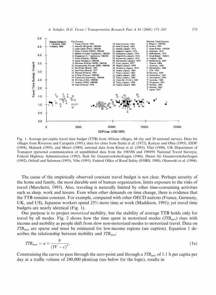
First, Zahavi proposed that, on average, humans spend a ®xed amount of their daily timebudget traveling ± the travel time budget (TTB). Time-use and travel surveys from numerous citiesand countries throughout the world suggest that TTB is approximately 1.1 h per person per day.Fig. 1 shows the stability of the travel time budget over a wide range of income levels, geo-graphical and cultural settings: residents of African villages devotesimilar time for travel as thoseof Japan, Singapore, Western Europe or North America.

While the TTB is constant on average, many variations are evident when examining thebehavior of small populations and individuals. Travel time budgets are higher in congestedcities; Londoners, for example, spend 30% more time traveling than do people in spaciousScotland (UK Department of Transport, personal communication of unpublished data of the1985/86 and 1989/91 National Travel Surveys). Fig. 1 shows that the magnitude and variance ofthe TTB in cities (open circles) are higher than average TTBs for whole countries (solid sym-bols). Travel times are generally highest for the largest cities (e.g. Paris). TTB also varies withsociodemographic group. A 1989 survey in West Germany (Kloas et al., 1993) illustrates thevariability of travel habits by profession ± the average person traveled 1.09 h per day, butuniversity students and government employees spent much more time in motion (1.27 and1.32 h, respectively). German pensioners were less mobile (0.94 h). Studies have shown thatTTB per traveler is typically higher at lower incomes (Roth and Zahavi, 1981). (A ``traveler'' isde®ned in travel surveys as someone making at least one motorized trip on the day of thesurvey.) The poor face more constraints on their choice of living locations and transport modesand thus ®nd it more di�cult to optimize travel times. The share of travelers to total populationis lower in low-income societies; thus the average per person TTB (as shown in Fig. 1) is similarto that of other, high-income societies. 2

2 In addition to those discussed here, many other factors (including di�erences in survey methods) a�ect the measured

TTB values. We have made extensive e�ort that the data discussed here and presented in Fig. 1 are based on

comparable survey methods. For example, we have excluded survey data from several Chinese cities because they

excluded short walking trips.


The cause of the empirically observed constant travel budget is not clear. Perhaps security ofthe home and family, the most durable unit of human organization, limits exposure to the risks oftravel (Marchetti, 1993). Also, traveling is naturally limited by other time-consuming activitiessuch as sleep, work and leisure. Even when other demands on time change, there is evidence thatthe TTB remains constant. For example, compared with other OECD nations (France, Germany,UK, and US), Japanese workers spend 25% more time at work (Maddison, 1991); yet travel timebudgets are nearly identical (Fig. 1).

Our purpose is to project motorized mobility, but the stability of average TTB holds only fortravel by all modes. Fig. 2 shows how the time spent in motorized modes (TTBmot) rises withincome and mobility as people shift from slow non-motorized modes to motorized travel. Data onTTBmot are sparse and must be estimated for low-income regions (see caption). Equation 1 de-scribes the relationship between mobility and TTBmot:

TTBmot � a� b

�TV ÿ c�d : �1a�

Constraining the curve to pass through the zero-point and through a TTBmot of 1.1 h per capita perday at a tra�c volume of 240,000 pkm/cap (see below for the logic), results in

Fig. 1. Average per-capita travel time budget (TTB) from African villages, 44 city and 20 national surveys. Data for

villages from Riverson and Carapetis (1991); data for cities from Szalai et al. (1972), Katiyar and Ohta (1993), EIDF

(1994), Malasek (1995), and Metr~o (1989); national data from Kloas et al. (1993), Vliet (1994), UK Department of

Transport (personal communication of unpublished data from the 1985/86 and 1989/91 National Travel Surveys),

Federal Highway Administration (1992), Stab f�ur Gesamtverkehrsfragen (1986), Dienst f�ur Gesamtverkehrsfragen

(1992), Orfeuil and Salomon (1993), Vibe (1993), Federal O�ce of Road Safety (FORS, 1988), Olszewski et al. (1994).


a � ÿ b

�ÿc�d �1b�

b � 1:1

1240; 000ÿ c� �d

� �ÿ 1ÿc� �d� � : �1c�

Manually iterating d for the best ®t yields d � 20 and c � ÿ176;083 (Standard Error 5061); R2 is0.9896.

2.2. Travel money budget

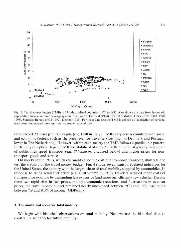
A second constant proposed by Zahavi is that individuals devote a ®xed proportion of incometo traveling, the travel money budget (TMB). Fig. 3 presents TMB time series data for 13 in-dustrialized countries (no other continuous time series surveys are available) and discrete pointsfor three developing countries. We are interested in the aggregate, stable budget, but some wellunderstood variations exist. As Zahavi (1981) observed, TMB rises with motorization (see alsoZahavi and Talvitie, 1980). Households without a personal car devote only 3±5% of income totraveling, which is illustrated by the three developing countries shown in Fig. 3. The rising TMBsfor Greece, Japan, Italy and Portugal in Fig. 3 illustrates the e�ect of increasing motorization.With increased ownership of cars the TMB rises until it stabilizes at 10±15% when motorization

Fig. 2. Travel time spent in motorized modes of transport (TTBmot) as a function of total mobility. Data for NAM,

PAO, WEU are from travel surveys in those regions. Estimates for the other eight regions are based on speeds used in

Table 3.


rates exceed 200 cars per 1000 capita (e.g. 1980 in Italy). TMBs vary across countries with socialand economic factors, such as the price level for travel services (high in Denmark and Portugal,lower in The Netherlands). However, within each society the TMB follows a predictable pattern.In the only exception, Japan, TMB has stabilized at only 7%, re¯ecting the atypically large shareof public high-speed transport (e.g. Shinkansen, discussed below) and higher prices for non-transport goods and services.

Oil shocks in the 1970s, which overnight raised the cost of automobile transport, illustrate andtest the stability of the travel money budget. Fig. 4 shows seven transport-related indicators forthe United States, the country with the largest share of total mobility supplied by automobiles. Inresponse to rising retail fuel prices (e.g. a 50% jump in 1979), travelers reduced other costs oftransport, for example by demanding less expensive (and more fuel e�cient) new vehicles. Despitethese two rapid rises in fuel prices, multiple economic recessions, and ¯uctuations in new carprices, the travel money budget remained nearly unchanged between 1970 and 1990, oscillatingbetween 7.9 and 9.0% of income (GDP/cap).

3. The model and scenario: total mobility

We begin with historical observations on total mobility. Next we use the historical data toconstrain a scenario for future mobility.

Fig. 3. Travel money budget (TMB) in 13 industrialized countries, 1970 to 1992. Also shown are data from household

expenditure surveys in three developing countries. Source: Eurostat (1994), Central Statistical O�ce (1970, 1980, 1990,

1993), Statistics Bureau (1972±1992), Deaton (1985). For these data sets the TMB is de®ned as the fraction of personal

transportation expenditures and total consumer expenditure.


3.1. Historical relationships

A predictable TMB allows us to posit a strong relationship between income and the totaldemand for mobility. As income rises, spending on travel must also increase ± the proportion isde®ned by the TMB. In turn, higher transport spending allows greater mobility. This relationshipbetween income and mobility can be quanti®ed. For income (GDP) data we employ the widelyused Penn World Tables, which report time-series estimates for all nations into constant 1985 USdollars (Summers et al., 1996). Appendix A provides more detail and caveats and compares thePenn World Tables with other available macroeconomic data. Mobility statistics are availablefrom national and industry statistical yearbooks, which one of us has compiled into a uniqueglobal data set (Schafer, 1998). 3 That complete historical (1960 to 1990) data set for all 11 regions

Fig. 4. Transport-related indicators in the US. TMB is stable over the period, despite two abrupt increases in real retail

prices of automobile fuel. TMB remained level as consumers compensated by purchasing new cars with lower fuel

consumption. Other indicators shown: real mean price and fuel consumption of sales-weighted new cars, annual dis-

tance traveled per car, per-capita mobility, and per-capita gross national product. Values normalized at 1970 levels; fuel

consumption normalized at 1973 as comparable earlier data for the US ¯eet are not available. Sources: Davis (1994),

Federal Highway Administration (1970±1991, 1992). TMB is computed from transportation personal consumption

expenditures divided by gross national product (Davis, 1994, Tables 2.28 and 2.27).

3 This paper includes some minor improvements to the Schafer (1998) data set. Most important, air tra�c data from

non-scheduled ¯ights between 1975 and 1990 are now derived from ICAO (1975±1991). We estimate data between 1960

and 1974 by assuming that the ratio of non scheduled tra�c volumes was ®x at the level observed between 1975 and

1990.


allows us to test the claim that the TMB de®nes a predictable quanti®ed relationship betweengrowth in income and total mobility. 4 The data also make possible statistical regressions that arethe tool of our model.

Fig. 5 shows the relationship between income (independent variable) and mobility (dependentvariable). In all ®ve of the regions with highest income ± Eastern Europe (EEU), former SovietUnion (FSU), North America (NAM), paci®c OECD nations (PAO), Western Europe (WEU) ±per-capita mobility and income have grown in essentially the same proportion, with slope� 1.This pattern exists despite a wide variety of di�erent regional and cultural settings. However, thereare signi®cant di�erences in absolute mobility; some regional trajectories lie above, others belowthe central trajectory of slope� 1 (dashed line). For example, at 10,000 USD per capita, per capitamobility in WEU was only 60% that of NAM, re¯ecting di�erent infrastructures, populationdensities, cultures, and unit costs of transport.

The six lower income regions show more variation, which re¯ects several factors. One factor isthat conversion of income statistics into common units is imperfect (see Appendix A). A secondfactor is the substitution of motorized transport for other modes, notably non-motorized forms(walking, bicycles, animal-drawn carts) and motorcycles ± data for those other modes are poorand not shown in Fig. 5. Such a substitution has been demonstrated in the replacement of horsesby automobiles in the US over a period of less than three decades beginning in the 1900s(Nakicenovic, 1988). We interpret the curvature of the growth in mobility in Paci®c Asia nations(PAS) in Fig. 5, for example, as evidence of such substitution; such curvature is not evident in alllow-income regions, probably because the extent of curvature also depends on the methods usedfor gathering and converting income data (see Appendix A). A third factor, deep economic re-cession, applies especially to Middle East and North Africa (MEA) and Sub-Saharan Africa(AFR). In these regions, economies contracted sharply in the 1980s although aggregate mobilitycontinued to rise, temporarily. As a result, the data show a hysteresis between economic recessionand demand for transport because earlier investments (the major share of transport costs)continue to enhance mobility in the early stages of recession. Latin America (LAM) experienced ashorter deep recession in the 1980s, leading to similar but less pronounced results. The earlierhistory of all three of these regions ± MEA, AFR, and LAM ± shows that during periods ofsustained growth, mobility rises with income.

3.2. Future mobility

Our projection of total mobility is a function of the stable TMB, which is the sum of two parts.One is the fraction of income allocated to mobility (TMBM). The other is the share devoted toquality of service ± comfort, style, safety, engine power (TMBS).

4 In principle, the rise in TMB from 3±5 to 10±15% with increasing motorization might allow for more rapid growth in

mobility because a larger fraction of income is devoted to travel. In practice, it appears that rising travel money budgets

are o�set completely by the rising unit cost of travel as travelers shift from public modes (bus, railroads) to private

automobile. Thus even at low mobility, there is a direct relationship between rising income and rising mobility. No data

exist to test exactly this relationship, but the tight correlation between income growth and total mobility o�ers a partial

test (and, most important, con®rms the aggregate relationship that is crucial to our forecast). See Fig. 5 and discussion

below.


Time series data from both the United States (Fig. 4) and Germany (Deutsche AutomobilTreuhand, 1994), for example, suggest that the two shares do not necessarily remain strictlyconstant over time. In both countries, the average real purchase price of new automobiles ± whichis a proxy for quality of service ± rose with rising per-capita income. In the US, both new carprices and income grew 40% between 1970 and 1990. In Germany, however, new car pricesdoubled while income rose only 52%; German car-buyers have devoted a growing share of in-come to quality of service and taxes. Data that illustrate the constancy of the TMB (e.g. Figs. 3and 4) are the sum of these two components; however, only TMBM is used to determine the re-lationship between income and mobility. The following simple equations describe the relation-ship.

Tra�c volume (TV ) per capita depends on (i) the money people spend on transport and (ii) theinverse unit cost of transport, v (units: pkm/USD). The ®rst of these factors can be expressed asthe product of income (GDP=cap) and the travel money budget (TMBM). The factor v depends onseveral economic and technological parameters of the employed modes of transport, such ascapital costs and fuel e�ciency. In the general case:

TVcap� GDP

cap� TMBM

� �� v: �2�

If historical data for each of the three variables on the right hand side were available we could useEq. (2) for estimating future levels of mobility. However time series data for travel money budgetand v are only available for a few countries. According to Fig. 5, the relationship between percapita mobility and per capita income can be approximated by:

Fig. 5. Scenario for mobility and income for 11 regions, 1991±2050. A hypothetical ``target point'', to which all tra-

jectories converge, is shown. For comparison, historical data (1960±1990) are shown with symbols.


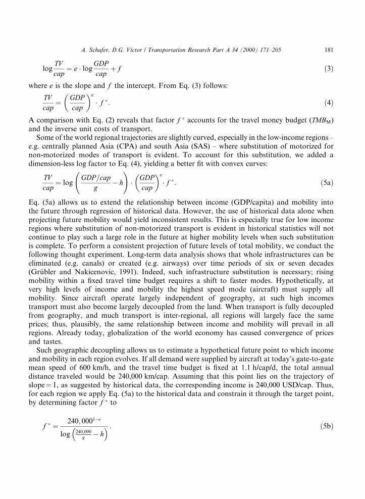
logTVcap� e � log

GDPcap� f �3�

where e is the slope and f the intercept. From Eq. (3) follows:

TVcap� GDP

cap

� �e

� f �: �4�

A comparison with Eq. (2) reveals that factor f � accounts for the travel money budget (TMBM)and the inverse unit costs of transport.

Some of the world regional trajectories are slightly curved, especially in the low-income regions ±e.g. centrally planned Asia (CPA) and south Asia (SAS) ± where substitution of motorized fornon-motorized modes of transport is evident. To account for this substitution, we added adimension-less log factor to Eq. (4), yielding a better ®t with convex curves:

TVcap� log

GDP=capg

ÿ h

!� GDP

cap

� �e

� f �: �5a�

Eq. (5a) allows us to extend the relationship between income (GDP/capita) and mobility intothe future through regression of historical data. However, the use of historical data alone whenprojecting future mobility would yield inconsistent results. This is especially true for low incomeregions where substitution of non-motorized transport is evident in historical statistics will notcontinue to play such a large role in the future at higher mobility levels when such substitutionis complete. To perform a consistent projection of future levels of total mobility, we conduct thefollowing thought experiment. Long-term data analysis shows that whole infrastructures can beeliminated (e.g. canals) or created (e.g. airways) over time periods of six or seven decades(Gr�ubler and Nakicenovic, 1991). Indeed, such infrastructure substitution is necessary; risingmobility within a ®xed travel time budget requires a shift to faster modes. Hypothetically, atvery high levels of income and mobility the highest speed mode (aircraft) must supply allmobility. Since aircraft operate largely independent of geography, at such high incomestransport must also become largely decoupled from the land. When transport is fully decoupledfrom geography, and much transport is inter-regional, all regions will largely face the sameprices; thus, plausibly, the same relationship between income and mobility will prevail in allregions. Already today, globalization of the world economy has caused convergence of pricesand tastes.

Such geographic decoupling allows us to estimate a hypothetical future point to which incomeand mobility in each region evolves. If all demand were supplied by aircraft at today's gate-to-gatemean speed of 600 km/h, and the travel time budget is ®xed at 1.1 h/cap/d, the total annualdistance traveled would be 240,000 km/cap. Assuming that this point lies on the trajectory ofslope� 1, as suggested by historical data, the corresponding income is 240,000 USD/cap. Thus,for each region we apply Eq. (5a) to the historical data and constrain it through the target point,by determining factor f � to

f � � 240; 0001ÿe

log 240;000g ÿ h

� � : �5b�


Inclusion of the historical data also helps to account for the many factors that determine the exactrelationship between income and mobility, such as the unit costs of transport, the particular valueof the TMB, and historical developments such as investments in transportation infrastructure.These factors change only slowly and thus each region's history constrains the exact developmentof total mobility.

We used Eqs. (5a) and (5b) for all regions except LAM, MEA, and AFR, where prolongedrecessions meant that historical growth in income has not been continuous. For those regions, weused Eq. (4) over the 1990 value and the target point. In CPA, this paper uses only the last twodecades of historical data; earlier data show an irregular oscillation of modal shares and appear tobe especially implausible. Parameter estimates, R-squared, and standard errors of all regressionequations are indicated in Appendix B.

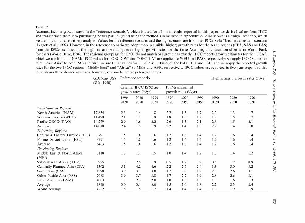
We have no model of the world economy, and thus we used growth rates based on the widelyused IS92a baseline scenario of the Intergovernmental Panel on Climate Change (IPCC/IS92a;Legget et al., 1992). However, that scenario employed growth rates in Asia that are below otherauthoritative scenarios (see review in Alcamo et al., 1995); thus, we used higher values (fromIPCC/IS92e) for the three Asian developing regions (CPA, PAS, SAS). The values that we usedfor the ``reference scenario'' presented in this paper are summarized in Table 2. Below we illustratethe sensitivity of our results to this crucial parameter ± income growth ± with a ``high scenario''that employs the even higher growth rates for Asia drawn from the World Bank (World Bank,1996), also shown in Table 2.

Fig. 5 also shows the regional projections and the ``target point''. Values for 1960, 1990, 2020and 2050 are shown in Table 3. None of the regions approaches the income and mobility levels ofthe target point by the year 2050, which is consistent with its use as a concept rather than a strictlyrealistic statement about the future. The target point is su�ciently distant in the future that itsspeci®c location on the central trajectory does not matter much (see the section ``Sensitivity of theResults'', below). NAM, the region where the projected income growth will be highest by 2050,would reach the target point only a century later (in 2160) if income kept growing at the samerates.

Calculating absolute levels of future mobility (Table 3) requires population estimates. Weused the 1992 World Bank projections, which estimate an increase in world population to 10.1billion in 2050 (Bos et al., 1992). In those projections, growth is strongest in developingcountries, where population more than doubles during the period and accounts for 85% ofworld population in 2050. These values are similar to the 1992 UN medium forecast (UnitedNations, 1992). 5

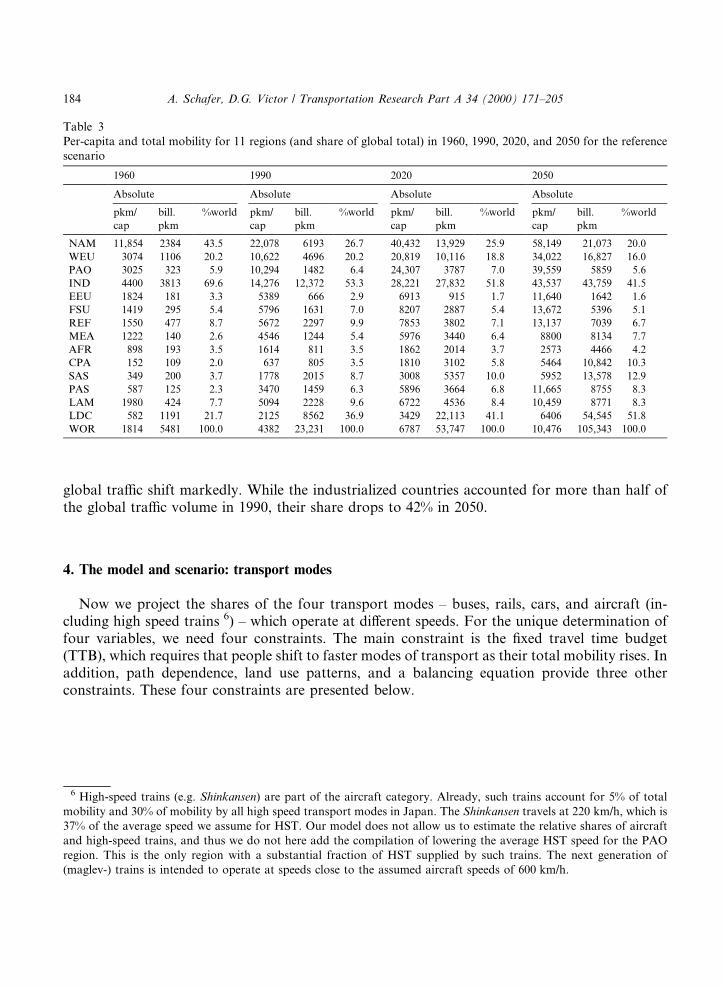
Based on Eqs. (5a) and (5b) and the assumed income growth rates we project that per capitatra�c volume will increase by a factor between 2.6 and 3.8 in the three regions of industrializedcountries; in developing regions the rise in mobility will be as much as nine-fold (CPA). Globally,in 2050, people will average an annual tra�c volume comparable to that of West European andPAO residents in 1990. The stronger growth in per capita mobility in the developing world isampli®ed by the largest absolute and relative growth in population. Hence, regional shares in

5 More recent forecasts include the 1996 World Bank (9.2 billion) and 1996 UN (short-term) medium projection (9.4

billion). For a review and some recent projections, see Lutz (1996).


Table 2

Assumed income growth rates. In the ``reference scenario'', which is used for all main results reported in this paper, we derived values from IPCC

and transformed them into purchasing power parities (PPP) using the method summarized in Appendix A. Also shown is a ``high'' scenario, which

we use only to for a sensitivity analysis. Values for the reference scenario and the high scenario are from the IPCC/IS92a ``business as usual'' scenario

(Leggett et al., 1992). However, in the reference scenario we adopt more plausible (higher) growth rates for the Asian regions (CPA, SAS and PAS)

from the IS92e scenario. In the high scenario we adopt even higher growth rates for the three Asian regions, based on short-term World Bank

forecasts (World Bank, 1996). The regional groupings for IPCC do not match our groupings exactly. IPCC reports growth estimates for the `ÙSA'',

which we use for all of NAM; IPCC values for `ÒECD-W'' and `ÒECD-A'' are applied to WEU and PAO, respectively; we apply IPCC values for

``Southeast Asia'' to both PAS and SAS; we use IPCC values for `ÙSSR & E. Europe'' for both EEU and FSU; and we apply the reported growth

rates for the two IPCC regions ``Middle East'' and `Àfrica'' to MEA and AFR, respectively. IPCC values are reported in ®ve-year steps, and this

table shows three decade averages; however, our model employs ten-year steps

GDP/cap US$

(Ô85) (1990)

Reference scenario High scenario growth rates (%/yr)

Original IPCC IS'92 a/e

growth rates (%/yr)

PPP-transformed

growth rates (%/yr)

1990

2020

2020

2050

1990

2050

1990

2020

2020

2050

1990

2050

1990

2020

2020

2050

1990

2050

Industrialized Regions

North America (NAM) 17,854 2.3 1.4 1.8 2.2 1.3 1.7 2.2 1.3 1.7

Western Europe (WEU) 11,499 2.1 1.7 1.9 1.8 1.5 1.7 1.8 1.5 1.7

Paci®c-OECD (PAO) 14,279 2.9 1.6 2.2 2.6 1.5 2.1 2.6 1.5 2.1

Average 14,018 2.4 1.5 1.9 2.2 1.4 1.8 2.2 1.4 1.8

Reforming Regions

Central & Eastern Europe (EEU) 3791 1.5 1.8 1.6 1.2 1.6 1.4 1.2 1.6 1.4

Former Soviet Union (FSU) 3791 1.5 1.8 1.6 1.2 1.6 1.4 1.2 1.6 1.4

Average 6463 1.5 1.8 1.6 1.2 1.6 1.4 1.2 1.6 1.4

Developing Regions

Middle East & North Africa

(MEA)

3118 1.3 1.7 1.5 1.0 1.4 1.2 1.0 1.4 1.2

Sub-Saharan Africa (AFR) 985 1.3 2.5 1.9 0.5 1.2 0.9 0.5 1.2 0.9

Centrally Planned Asia (CPA) 1392 5.1 4.2 4.6 2.2 2.7 2.4 3.3 3.0 3.2

South Asia (SAS) 1298 3.9 3.7 3.8 1.7 2.2 1.9 2.8 2.6 3.1

Other Paci®c Asia (PAS) 2983 3.9 3.7 3.8 1.7 2.2 1.9 2.8 2.6 3.1

Latin America (LAM) 4083 1.7 2.3 2.0 1.0 1.6 1.3 1.0 1.6 1.3

Average 1890 3.0 3.1 3.0 1.5 2.0 1.8 2.2 2.3 2.4

World Average 4222 1.8 1.5 1.7 1.4 1.4 1.4 1.9 1.9 1.9

A.

Sch

afer,

D.G

.V

ictor

/T

ran

spo

rtatio

nR

esearch

Pa

rtA

34

(2

00

0)

17

1±

20

51

83

global tra�c shift markedly. While the industrialized countries accounted for more than half ofthe global tra�c volume in 1990, their share drops to 42% in 2050.

4. The model and scenario: transport modes

Now we project the shares of the four transport modes ± buses, rails, cars, and aircraft (in-cluding high speed trains 6) ± which operate at di�erent speeds. For the unique determination offour variables, we need four constraints. The main constraint is the ®xed travel time budget(TTB), which requires that people shift to faster modes of transport as their total mobility rises. Inaddition, path dependence, land use patterns, and a balancing equation provide three otherconstraints. These four constraints are presented below.

Table 3

Per-capita and total mobility for 11 regions (and share of global total) in 1960, 1990, 2020, and 2050 for the reference

scenario

1960 1990 2020 2050

Absolute Absolute Absolute Absolute

pkm/

cap

bill.

pkm

%world pkm/

cap

bill.

pkm

%world pkm/

cap

bill.

pkm

%world pkm/

cap

bill.

pkm

%world

NAM 11,854 2384 43.5 22,078 6193 26.7 40,432 13,929 25.9 58,149 21,073 20.0

WEU 3074 1106 20.2 10,622 4696 20.2 20,819 10,116 18.8 34,022 16,827 16.0

PAO 3025 323 5.9 10,294 1482 6.4 24,307 3787 7.0 39,559 5859 5.6

IND 4400 3813 69.6 14,276 12,372 53.3 28,221 27,832 51.8 43,537 43,759 41.5

EEU 1824 181 3.3 5389 666 2.9 6913 915 1.7 11,640 1642 1.6

FSU 1419 295 5.4 5796 1631 7.0 8207 2887 5.4 13,672 5396 5.1

REF 1550 477 8.7 5672 2297 9.9 7853 3802 7.1 13,137 7039 6.7

MEA 1222 140 2.6 4546 1244 5.4 5976 3440 6.4 8800 8134 7.7

AFR 898 193 3.5 1614 811 3.5 1862 2014 3.7 2573 4466 4.2

CPA 152 109 2.0 637 805 3.5 1810 3102 5.8 5464 10,842 10.3

SAS 349 200 3.7 1778 2015 8.7 3008 5357 10.0 5952 13,578 12.9

PAS 587 125 2.3 3470 1459 6.3 5896 3664 6.8 11,665 8755 8.3

LAM 1980 424 7.7 5094 2228 9.6 6722 4536 8.4 10,459 8771 8.3

LDC 582 1191 21.7 2125 8562 36.9 3429 22,113 41.1 6406 54,545 51.8

WOR 1814 5481 100.0 4382 23,231 100.0 6787 53,747 100.0 10,476 105,343 100.0

6 High-speed trains (e.g. Shinkansen) are part of the aircraft category. Already, such trains account for 5% of total

mobility and 30% of mobility by all high speed transport modes in Japan. The Shinkansen travels at 220 km/h, which is

37% of the average speed we assume for HST. Our model does not allow us to estimate the relative shares of aircraft

and high-speed trains, and thus we do not here add the compilation of lowering the average HST speed for the PAO

region. This is the only region with a substantial fraction of HST supplied by such trains. The next generation of

(maglev-) trains is intended to operate at speeds close to the assumed aircraft speeds of 600 km/h.


4.1. Path dependence and railways

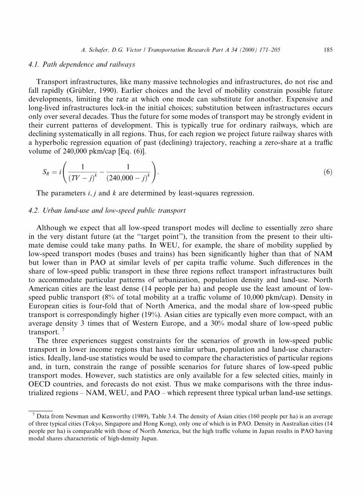
Transport infrastructures, like many massive technologies and infrastructures, do not rise andfall rapidly (Gr�ubler, 1990). Earlier choices and the level of mobility constrain possible futuredevelopments, limiting the rate at which one mode can substitute for another. Expensive andlong-lived infrastructures lock-in the initial choices; substitution between infrastructures occursonly over several decades. Thus the future for some modes of transport may be strongly evident intheir current patterns of development. This is typically true for ordinary railways, which aredeclining systematically in all regions. Thus, for each region we project future railway shares witha hyperbolic regression equation of past (declining) trajectory, reaching a zero-share at a tra�cvolume of 240,000 pkm/cap [Eq. (6)].

SR � i1

�TV ÿ j�k

ÿ 1

�240;000ÿ j�k!: �6�

The parameters i; j and k are determined by least-squares regression.

4.2. Urban land-use and low-speed public transport

Although we expect that all low-speed transport modes will decline to essentially zero sharein the very distant future (at the ``target point''), the transition from the present to their ulti-mate demise could take many paths. In WEU, for example, the share of mobility supplied bylow-speed transport modes (buses and trains) has been signi®cantly higher than that of NAMbut lower than in PAO at similar levels of per capita tra�c volume. Such di�erences in theshare of low-speed public transport in these three regions re¯ect transport infrastructures builtto accommodate particular patterns of urbanization, population density and land-use. NorthAmerican cities are the least dense (14 people per ha) and people use the least amount of low-speed public transport (8% of total mobility at a tra�c volume of 10,000 pkm/cap). Density inEuropean cities is four-fold that of North America, and the modal share of low-speed publictransport is correspondingly higher (19%). Asian cities are typically even more compact, with anaverage density 3 times that of Western Europe, and a 30% modal share of low-speed publictransport. 7

The three experiences suggest constraints for the scenarios of growth in low-speed publictransport in lower income regions that have similar urban, population and land-use character-istics. Ideally, land-use statistics would be used to compare the characteristics of particular regionsand, in turn, constrain the range of possible scenarios for future shares of low-speed publictransport modes. However, such statistics are only available for a few selected cities, mainly inOECD countries, and forecasts do not exist. Thus we make comparisons with the three indus-trialized regions ± NAM, WEU, and PAO ± which represent three typical urban land-use settings.

7 Data from Newman and Kenworthy (1989), Table 3.4. The density of Asian cities (160 people per ha) is an average

of three typical cities (Tokyo, Singapore and Hong Kong), only one of which is in PAO. Density in Australian cities (14

people per ha) is comparable with those of North America, but the high tra�c volume in Japan results in PAO having

modal shares characteristic of high-density Japan.


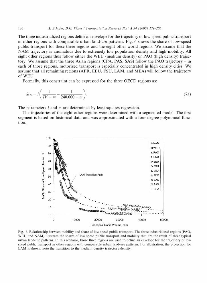
The three industrialized regions de®ne an envelope for the trajectory of low-speed public transportin other regions with comparable urban land-use patterns. Fig. 6 shows the share of low-speedpublic transport for these three regions and the eight other world regions. We assume that theNAM trajectory is anomalous due to extremely low population density and high mobility. Alleight other regions thus follow either the WEU (medium density) or PAO (high density) trajec-tory. We assume that the three Asian regions (CPA, PAS, SAS) follow the PAO trajectory ± ineach of those regions, motorized transport is especially concentrated in high density cities. Weassume that all remaining regions (AFR, EEU, FSU, LAM, and MEA) will follow the trajectoryof WEU.

Formally, this constraint can be expressed for the three OECD regions as:

SLS � l1

TV ÿ m

�ÿ 1

240;000ÿ m

�: �7a�

The parameters l and m are determined by least-squares regression.The trajectories of the eight other regions were determined with a segmented model. The ®rst

segment is based on historical data and was approximated with a four-degree polynomial func-tion:

Fig. 6. Relationship between mobility and share of low-speed public transport. The three industrialized regions (PAO,

WEU and NAM) illustrate the shares of low speed public transport and mobility that are the result of three typical

urban land-use patterns. In this scenario, those three regions are used to de®ne an envelope for the trajectory of low

speed public transport in other regions with comparable urban land-use patterns. For illustration, the projection for

LAM is shown; note the transition to the medium density trajectory density.


SLS � n� o � TV � p � TV 2 � q � TV 3 � r � TV 4: �7b�That ®rst segment converges to the second segment, which is the trajectory based on the ap-propriate OECD ``lead'' region [i.e. Eq. (7a)]. To achieve this convergence, the coe�cients n and owere determined by equating Eq. (7b) (®rst segment) to Eq. (7a) (second segment) at the point tv0

where both the functional value and the ®rst derivative of both equations are equal. Substitutingthe expressions for n and o in Eq. (7b) results in:

SLS � ltv0 ÿ m

1

�� TV ÿ tv0

mÿ tv0

�� p � �TV ÿ tv0�2 � q � �TV 3 ÿ 3tv2

0TV � 2tv30�

� r � �TV 4 ÿ 4tv30TV � 3tv4

0�: �7c�The parameters p; q; r and the tra�c volume at the point of convergence between the two segments�tv0� were determined through least-squares regression. For illustration of the segmented model,Fig. 6 shows the computed transition paths for the LAM region, which follows the trajectory ofmedium density.

Because rail shares are already determined [Eq. (6)], the share for bus travel results from:

SB � SLS ÿ SR �8�

4.3. Travel time budget

A ®xed travel time budget requires that the mean speed of travel increases in proportion to theprojected rise in total per capita mobility. More distance must be covered within the same periodof time. Since transport carriers only operate within a range of speeds, rising mean speed requiresshifting to faster transport modes.

Formally, the sum of the daily motorized per capita travel time �TT � over all modes of transport(i) which move daily tra�c volume (TVi) at mean speed (Vi), must equal the travel time budget formotorized modes (TTBmot):X

i

TTi �X

i

TVi

Vi� TTBmot: �9�

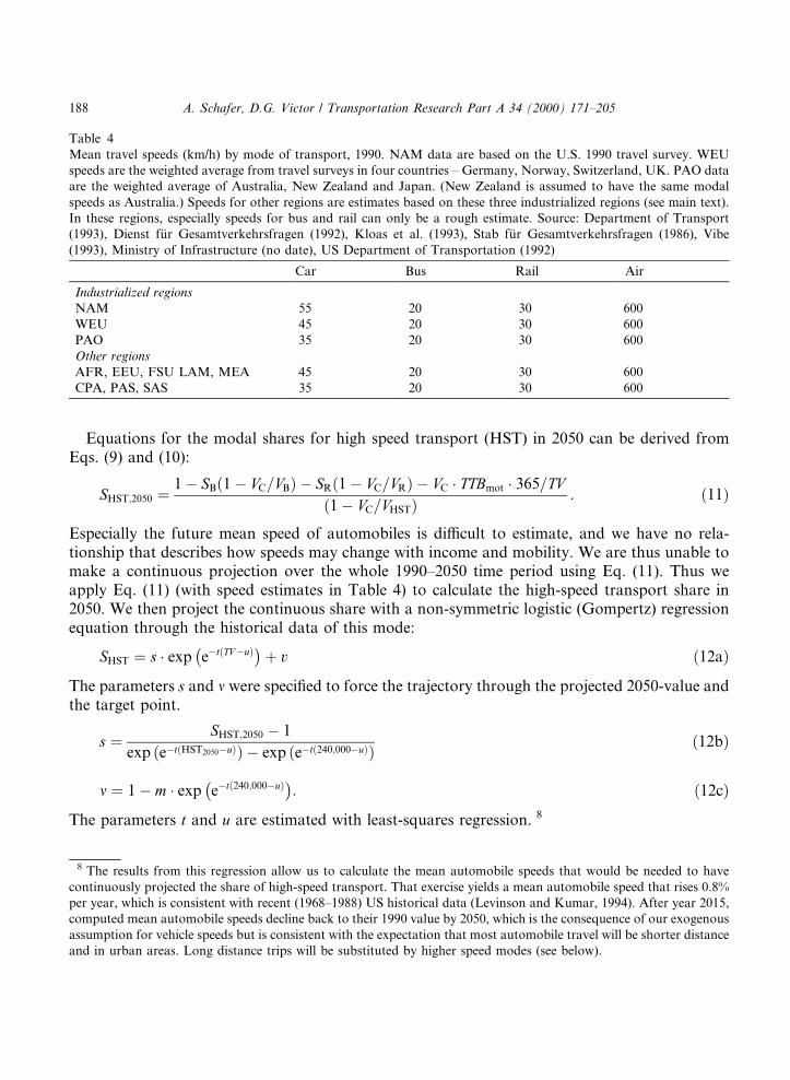
Applying the TTB constraint from Eq. (9) requires that we estimate the mean speed of eachtravel mode. Table 4 summarizes available travel survey data in three world regions ± NAM, PAOand WEU ± which we used to estimate future speeds in other regions. The table shows that themean speed of buses, trains and aircraft are identical in the three regions; we assumed that thesame speeds apply to all other regions as well. In contrast, the mean speed of car travel varies byregion. We derive TTBmot from Eqs. (1a)±(1c).

4.4. Balancing equation ± total tra�c volume

The fourth constraint is that the tra�c volume of each motorized mode (i) must sum to thetotal projected tra�c volume for each region:

TV �X

i

TVi : �10�


Equations for the modal shares for high speed transport (HST) in 2050 can be derived fromEqs. (9) and (10):

SHST;2050 � 1ÿ SB�1ÿ VC=VB� ÿ SR�1ÿ VC=VR� ÿ VC � TTBmot � 365=TV�1ÿ VC=VHST� : �11�

Especially the future mean speed of automobiles is di�cult to estimate, and we have no rela-tionship that describes how speeds may change with income and mobility. We are thus unable tomake a continuous projection over the whole 1990±2050 time period using Eq. (11). Thus weapply Eq. (11) (with speed estimates in Table 4) to calculate the high-speed transport share in2050. We then project the continuous share with a non-symmetric logistic (Gompertz) regressionequation through the historical data of this mode:

SHST � s � exp eÿt�TVÿu�ÿ �� v �12a�The parameters s and m were speci®ed to force the trajectory through the projected 2050-value andthe target point.

s � SHST;2050 ÿ 1

exp eÿt�HST2050ÿu�� ÿ exp eÿt�240;000ÿu�� 12b�

m � 1ÿ m � exp eÿt�240;000ÿu�ÿ �: �12c�

The parameters t and u are estimated with least-squares regression. 8

8 The results from this regression allow us to calculate the mean automobile speeds that would be needed to have

continuously projected the share of high-speed transport. That exercise yields a mean automobile speed that rises 0.8%

per year, which is consistent with recent (1968±1988) US historical data (Levinson and Kumar, 1994). After year 2015,

computed mean automobile speeds decline back to their 1990 value by 2050, which is the consequence of our exogenous

assumption for vehicle speeds but is consistent with the expectation that most automobile travel will be shorter distance

and in urban areas. Long distance trips will be substituted by higher speed modes (see below).

Table 4

Mean travel speeds (km/h) by mode of transport, 1990. NAM data are based on the U.S. 1990 travel survey. WEU

speeds are the weighted average from travel surveys in four countries ± Germany, Norway, Switzerland, UK. PAO data

are the weighted average of Australia, New Zealand and Japan. (New Zealand is assumed to have the same modal

speeds as Australia.) Speeds for other regions are estimates based on these three industrialized regions (see main text).

In these regions, especially speeds for bus and rail can only be a rough estimate. Source: Department of Transport

(1993), Dienst f�ur Gesamtverkehrsfragen (1992), Kloas et al. (1993), Stab f�ur Gesamtverkehrsfragen (1986), Vibe

(1993), Ministry of Infrastructure (no date), US Department of Transportation (1992)

Car Bus Rail Air

Industrialized regions

NAM 55 20 30 600

WEU 45 20 30 600

PAO 35 20 30 600

Other regions

AFR, EEU, FSU LAM, MEA 45 20 30 600

CPA, PAS, SAS 35 20 30 600


Finally, we can derive the share of automobile travel SC:

SC � 1ÿ SLS ÿ SHST: �13�

4.5. High-speed niche markets

In principle, we could derive all regional projections for HST shares from Eq. (11). All terms inthat equation are determined by exogenous speed assumptions or calculations, except the ®nalterm in the numerator. The value of that term depends on the value of TTBmot; Fig. 2 shows thatTTBmot is especially sensitive in regions with low income (low tra�c volume). For example, re-ducing TTBmot in NAM in 2050 by 10% would only incur a 6% increase in the modal share of high-speed transportation, whereas the same change in SAS would result in a 56% increase. Moreover,data on modal speeds and TTBmot are practically non-existent in those regions and thus it would beinappropriate to use this method. Setting the ®rst derivative of Eq. (11) (i.e. dSHST;2050=dTTBmot) to)1 allows us to calculate the threshold tra�c volume at which a change in TTBmot by one unitresults in an equal unit change in SHST;2050. Mean car speed varies by region and thus the calculatedthreshold value also varies: 24,340 pkm/cap in NAM; 17,750 pkm/cap for WEU, AFR, EEU,FSU, LAM, MEA; and 13,560 pkm/cap for PAO, CPA, PAS, SAS. Only in the three OECDregions (NAM, PAO, and WEU) are the projected 2050 levels above that threshold (see Table 3);using this criterion, we can apply Eq. (11) only for these three regions.

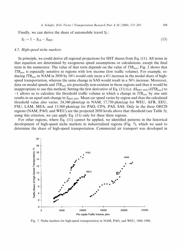
For other regions, where Eq. (11) cannot be applied, we identi®ed patterns in the historicaldevelopment of high-speed niche markets in industrialized regions (Fig. 7), which we used todetermine the share of high-speed transportation. Commercial air transport was developed in

Fig. 7. Niche markets for high-speed transportation in NAM, PAO, and WEU, 1960±1990.


North America; in that region, the rate of growth has been comparatively slow but will last overa long period. In regions where high-speed technology was introduced later, innovationspioneered in the lead regions were less costly and adopted more readily, which allowed more rapidgrowth in the niche market. Other factors that a�ect demand include the length of trips andpolicies that have altered market share, such as government subsidies. The data (Fig. 7) suggesttwo possibilities ± in Western Europe the rate of adoption (expressed as share of high-speedtransport as a function of total tra�c volume) was similar to that of North America. In PAOhigh-speed modes grew more rapidly ± dense human settlement impeded the use of road-basedtransportation for long-distance trips, and government subsidy of Shinkansen encouraged riders.We applied these growth rates in the niche markets for the calculation of the 2050 share with thesame regional correspondence as with the urban land-use constraint. Formally, the equation canbe written as:

SHST;2050 � SHST;1990 � w�TV2050ÿTV1990�: �14�The niche market approach [Eq. (14)] applies only in regions where the share of HST is typical

of a niche market, which we assume is approximately 5% of the 1990 tra�c volume. In addition toNAM, PAO and WEU, two other regions exceed that level: FSU (14.4%) and PAS (7.5%). Forthose regions, we apply Eq. (11). In the later section on ``Sensitivity of Results'' we vary thefactors that a�ect Eq. (11) (transport speeds and TTBmot) to check the sensitivity of the 2050 HSTshare. That analysis con®rms that for these ®ve regions (FSU, NAM, PAO, PAS, and WEU) it isappropriate to use Eq. (11).

4.6. Results

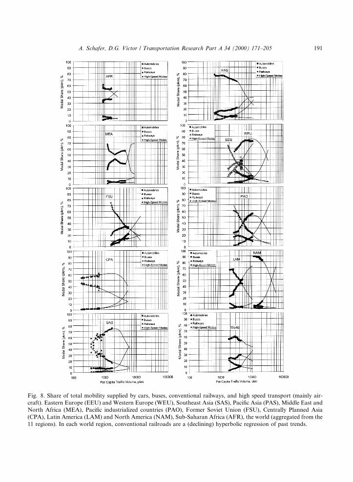
Together, these constraints de®ne unique values for each mode in each region. Fig. 8 presentseach of the regional projections.

Fig. 8 also reports the results aggregated at the world level. By 2050, only the share of aircraft isgrowing; all other modes are in relative decline. Aircraft provide 36% of global mobility in 2050;automobiles supply 42%. In all three industrialized countries, automobile shares decline sharplyby 2050. Rising automobility in developing countries is unable to o�set fully the automobile'srelative decline in other regions for several reasons: (a) income levels remain low in AFR andCPA, and thus automobility remains modest in these regions; (b) higher population densities leadto a lower saturation level for automobiles; and, (c) high shares of air travel supplant some of thepotential share of automobiles.

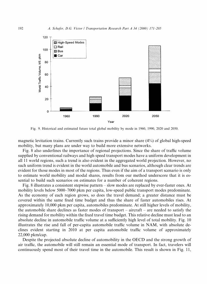
Fig. 9 shows absolute mobility levels for each mode in 1960, 1990, 2020 and 2050. In light of thefour fold rise in total mobility, the absolute mobility by each mode increases even for modes thatare in relative decline. Absolute mobility by car increases 260%. High speed mobility rises to28 times its 1990 level.

Such a strong increase in air travel may appear unrealistic because the airway network is alreadydense and congested in some regions. However, many technological possibilities are feasible andcan easily ®nd widespread application within six decades. Aircraft can be bigger ± carriers with acapacity of 1000 people are technologically feasible before 2020 (e.g. Covert et al., 1992). In ad-dition, our scenario for `àircraft'' consists of all high-speed modes operating at an average speed of600 km/h, which may include surface-bound high speed transport modes, such as wheel-on-rail and


Fig. 8. Share of total mobility supplied by cars, buses, conventional railways, and high speed transport (mainly air-

craft). Eastern Europe (EEU) and Western Europe (WEU), Southeast Asia (SAS), Paci®c Asia (PAS), Middle East and

North Africa (MEA), Paci®c industrialized countries (PAO), Former Soviet Union (FSU), Centrally Planned Asia

(CPA), Latin America (LAM) and North America (NAM), Sub-Saharan Africa (AFR), the world (aggregated from the

11 regions). In each world region, conventional railroads are a (declining) hyperbolic regression of past trends.


magnetic levitation trains. Currently such trains provide a minor share (4%) of global high-speedmobility, but many plans are under way to build more extensive networks.

Fig. 8 also underlines the importance of regional projections. Since the share of tra�c volumesupplied by conventional railways and high speed transport modes have a uniform development inall 11 world regions, such a trend is also evident in the aggregated world projection. However, nosuch uniform trend is evident in the world automobile and bus scenarios, although clear trends areevident for those modes in most of the regions. Thus even if the aim of a transport scenario is onlyto estimate world mobility and modal shares, results from our method underscore that it is es-sential to build such scenarios on estimates for a number of coherent regions.

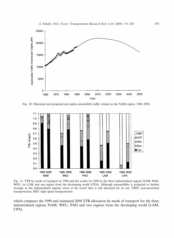
Fig. 8 illustrates a consistent stepwise pattern ± slow modes are replaced by ever-faster ones. Atmobility levels below 5000±7000 pkm per capita, low-speed public transport modes predominate.As the economy of each region grows, so does the travel demand; a greater distance must becovered within the same ®xed time budget and thus the share of faster automobiles rises. Atapproximately 10,000 pkm per capita, automobiles predominate. At still higher levels of mobility,the automobile share declines as faster modes of transport ± aircraft ± are needed to satisfy therising demand for mobility within the ®xed travel time budget. This relative decline must lead to anabsolute decline in automobile tra�c volume at a su�ciently high level of total mobility. Fig. 10illustrates the rise and fall of per-capita automobile tra�c volume in NAM, with absolute de-clines evident starting in 2010 at per capita automobile tra�c volume of approximately22,000 pkm/cap.

Despite the projected absolute decline of automobility in the OECD and the strong growth ofair tra�c, the automobile will still remain an essential mode of transport. In fact, travelers willcontinuously spend most of their travel time in the automobile. This result is shown in Fig. 11,

Fig. 9. Historical and estimated future total global mobility by mode in 1960, 1990, 2020 and 2050.


which compares the 1990 and estimated 2050 TTB allocation by mode of transport for the threeindustrialized regions NAM, WEU, PAO and two regions from the developing world (LAM,CPA).

Fig. 11. TTB by mode of transport in 1990 and the results for 2050 in the three industrialized regions NAM, PAO,

WEU, in LAM and one region from the developing world (CPA). Although automobility is projected to decline

strongly in the industrialized regions, most of the travel time is still allocated for its use. NMT: non-motorized

transportation; HST: high speed transportation.

Fig. 10. Historical and projected per-capita automobile tra�c volume in the NAM region, 1960±2050.


5. Consistency of results

For the developing world our results imply rapid di�usion of the automobile. For all regions,especially in industrialized and reforming regions, our scenario envisions large increases in highspeed mobility. Here we check whether those results are plausible ± we compare the rise ofautomobility with historical patterns; and, we check that the predominance of high speed travel inthe industrialized world is consistent with requirements for short distance travel (e.g. localshopping), where slow modes are likely to remain preferable.

5.1. Consistency with the historical motorization trends

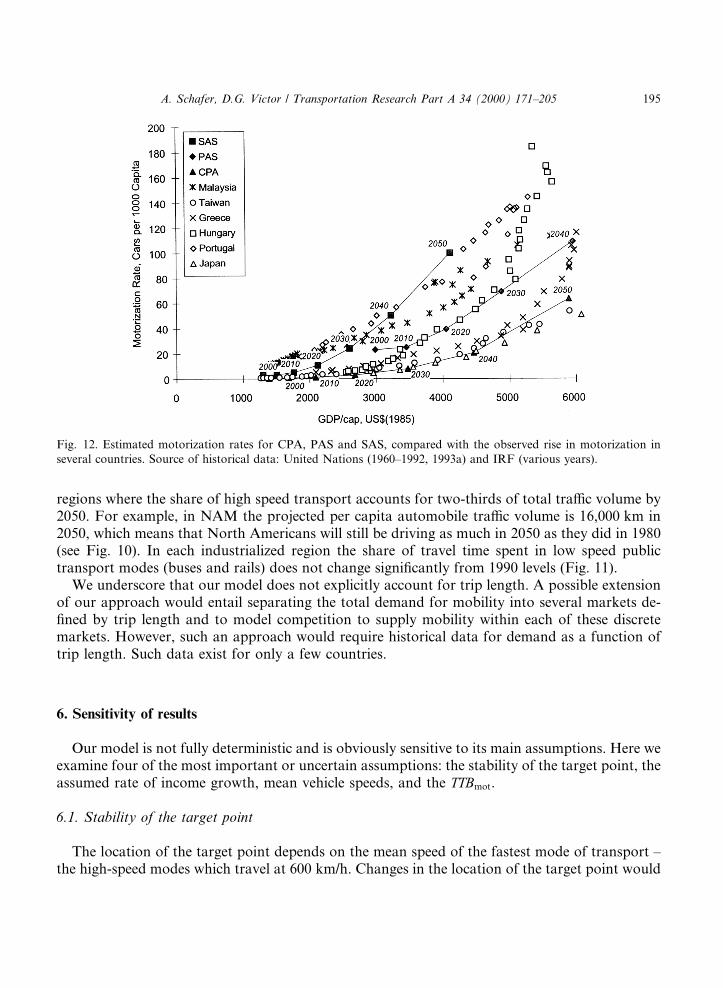
Unlike conventional forecasting methods, where motorization rates (passenger cars per capita)are a model input variable, our method allows calculation of motorization rates as an outputvariable. That computation requires the per-capita tra�c volume supplied by automobiles (cal-culated by the model) and two assumptions: a passenger load-factor and the annual distancedriven per vehicle. The projected motorization rates for developing countries can then be com-pared with historical trends in industrialized countries as a test of the consistency of the modeloutput. We apply this consistency check to CPA, PAS, and SAS ± the three Asian developingregions which have the highest projected GDP growth and will have strong substitution of au-tomobiles for other transport modes over the period of our projection.

We expect that load factors will decrease with rising incomes, as has been observed historicallyin nearly all countries. In 1990 the load factor was about 2.5 occupants per vehicle in SAS andCPA and 2.3 in PAS (Schafer, 1998). We estimate an exponentially decreasing curve de®ned bydata series from the US (Federal Highway Administration, 1992), UK (Department of Transport,1988, 1993), The Netherlands (Central Bureau voor de Statistiek, 1978±1993), New Zealand(Jollands, 1995), Switzerland (Dienst f�ur Gesamtverkehrsfragen, 1992), Australia (FORS, 1988),and Germany (Deutsches Institut f�ur Wirtschaftsforschung, 1991, 1993). Dividing the projectedworld-regional tra�c volume of passenger cars by the load factor and then by the estimateddistance traveled per vehicle (from Schafer, 1998) delivers estimates of motorization rates. Fig. 12shows that the motorization rates of the three regions, which rise with income, are broadlyconsistent with those of industrialized regions. The di�erence in motorization rates (high in SAS,low in CPA) are a result of the di�erent levels of mobility at a given income level (see Fig. 5) and,in turn, a consequence of the PPP-adjustments of the macroeconomic data set. However, we mayunderestimate motorization in CPA because the historical data set that we use does not extendbeyond 1990 and thus excludes the marked increase in motorization evident in the early 1990s(SSB, 1996).

5.2. Short distance travel

If the hypothetical ``target point'' were reached, high speed transport modes would account for100% market share. However, high speed modes are impractical for short trips, such as shoppingand travel to high speed nodes. Thus even at very high mobility levels, low speed modes must retainsome share of total mobility. We have checked that all projections are consistent with plausibleestimates for such short distance niche markets, with particular attention to the industrialized


regions where the share of high speed transport accounts for two-thirds of total tra�c volume by2050. For example, in NAM the projected per capita automobile tra�c volume is 16,000 km in2050, which means that North Americans will still be driving as much in 2050 as they did in 1980(see Fig. 10). In each industrialized region the share of travel time spent in low speed publictransport modes (buses and rails) does not change signi®cantly from 1990 levels (Fig. 11).

We underscore that our model does not explicitly account for trip length. A possible extensionof our approach would entail separating the total demand for mobility into several markets de-®ned by trip length and to model competition to supply mobility within each of these discretemarkets. However, such an approach would require historical data for demand as a function oftrip length. Such data exist for only a few countries.

6. Sensitivity of results

Our model is not fully deterministic and is obviously sensitive to its main assumptions. Here weexamine four of the most important or uncertain assumptions: the stability of the target point, theassumed rate of income growth, mean vehicle speeds, and the TTBmot.

6.1. Stability of the target point

The location of the target point depends on the mean speed of the fastest mode of transport ±the high-speed modes which travel at 600 km/h. Changes in the location of the target point would

Fig. 12. Estimated motorization rates for CPA, PAS and SAS, compared with the observed rise in motorization in

several countries. Source of historical data: United Nations (1960±1992, 1993a) and IRF (various years).


alter the development of the world-regional trajectories and thus the projected tra�c volume. Totest the sensitivity of the projections of total mobility, we examined an extreme case: reducing themean speed of the high-speed transport modes by one-third, to 400 km/h. This reduction causes aproportional shift in the target point from 240,000 to 160,000 pkm/cap. As a result, the projectedtra�c volume in 2050 declines by merely 1.5% in North America. The sensitivity of the other 10world regions is comparably low.

6.2. Income growth

The pattern of high speed transport modes replacing slower forms, and the dynamics that areparticular to each region, are robust derivations from the concepts of travel time budget and pathdependence. But the particular levels of mobility are mainly a function of income growth, which isexogenous to our model. Here we illustrate the sensitivity using a set of higher growth rates for thethree Asian developing regions (CPA, PAS, SAS) derived from World Bank forecasts (Table 1).These higher rates yield a global income in 2050 that is 34% higher than in our reference scenario.World mobility increases by a factor of 5.8, only 29% higher than the reference scenario. Thedi�erence between income and mobility re¯ects that although regional per capita mobility risesalmost directly with regional per capita income in 11 regions, both variables contribute withdi�erent shares to the world economy and tra�c volume. The sources of these di�erences includePPP-adjustments of the macro-economic data set (see Appendix A), which both shift and in¯u-ence the shape of the projected total mobility curve. In 1990, the CPA region contributes 3.5% tothe global motorized tra�c volume, but its share of world GDP is almost twice as high (6.7%).

Increasing the income growth rates also a�ects the mode of transport. With higher mobility anda ®xed travel time budget, travelers shift earlier to faster modes. In CPA and SAS automobilessubstitute for buses; in PAS, where income and mobility are comparatively higher, more rapidgrowth in income leads to substantially greater use of high-speed transport. Globally, many ofthese regional di�erences o�set. With high income growth rates, automobiles and high-speedtransport account for 40% and bus travel declines to 14% of the tra�c volume in 2050. Ourreference scenario envisions only slightly di�erent shares for buses (18%), high-speed transport(36%) and automobiles (42%).

6.3. Mean vehicle speeds and TTBmot

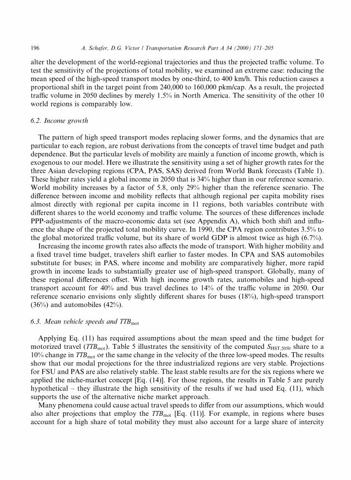
Applying Eq. (11) has required assumptions about the mean speed and the time budget formotorized travel (TTBmot). Table 5 illustrates the sensitivity of the computed SHST;2050 share to a10% change in TTBmot or the same change in the velocity of the three low-speed modes. The resultsshow that our modal projections for the three industrialized regions are very stable. Projectionsfor FSU and PAS are also relatively stable. The least stable results are for the six regions where weapplied the niche-market concept [Eq. (14)]. For those regions, the results in Table 5 are purelyhypothetical ± they illustrate the high sensitivity of the results if we had used Eq. (11), whichsupports the use of the alternative niche market approach.

Many phenomena could cause actual travel speeds to di�er from our assumptions, which wouldalso alter projections that employ the TTBmot [Eq. (11)]. For example, in regions where busesaccount for a high share of total mobility they must also account for a large share of intercity


tra�c and thus probably operate at speeds higher than the values we have assumed. For example,increasing the bus speeds by 50% (to 30 km/h, equal to that of railways) in PAS would reduce theHST share from 34 to 19% and increase the 2050 automobile share by nearly half, from 38 to 54%.Thus, for this region, we have probably underestimated the future share of automobile tra�c andover-stated the share of high-speed transport. A priority for future research is to make moreprecise estimates of vehicle speeds for each world region.

Results could also be a�ected by the introduction of intelligent transportation systems (ITS),such as timed-entry freeways and on-board tra�c directors that could reduce congestion andincrease the mean speed of automobiles by up to 15% (e.g. Diebold Institute for Public PolicyStudies, 1995). Consequently the share of automobiles would rise as this mode could, with ITS,better satisfy the demand for higher speed transport. Nonetheless, if automobile mean speedsincrease by 15%, our results are not radically altered. In NAM, for example, ITS would increasethe 2050 automobile tra�c share from 28 to 32%. However, as high-speed modes are still oneorder of magnitude swifter, the decline of automobiles would be delayed by only approximately4 years.

7. Conclusions

On average, people spend a constant share of money on traveling; rising income leads nearlydirectly to rising demand for mobility, which we demonstrate historically. A person also spends aconstant share of time for travel on average; as total mobility rises, travelers shift to faster modesto remain within the ®xed travel time budget of 1.1 h per person per day. In addition to theseconstant budgets, travel behavior is also a�ected by the path dependence of infrastructures, land-use constraints, and the development of niche markets. We use these factors to develop a newtechnique for projecting future mobility and mode of transport in all 11 world regions from 1990

Table 5

Decline in the computed share of HST in 2050 if equation (11) were applied to all regions. Numbers are the percentage

decline due to increasing the speeds for buses, or railways, or automobiles or TTBmot by 10%

Bus Rail Car TTBmot

Equation (11) used in this paper

North America (NAM) 0.4 0.0 4.2 5.8

Western Europe (WEU) 0.9 0.9 7.2 10

Paci®c-OECD (PAO) 1.1 0.4 2.7 5.0

Former Soviet Union (FSU) 11 13 27 54

Other Paci®c Asia (PAS) 12 0.9 12 27

Equation (14) used in this paper

Central & Eastern Eurpoe (EEU) 29 23 95 153

Middle East & North Africa (MEA) 61 4.9 156 226

Sub-Saharan Africa (AFR) 34 2.3 34 73

Centrally Planned Asia (CPA) 43 10 21 80

South Asia (SAS) 37 5.2 17 64

Latin America (LAM) 144 6.8 235 418


to 2050. This projection is made possible not only by the method presented in this paper butalso by the availability of a new historical data set (1960±1990) for all major motorized travelmodes.

All world regions illustrate the same phenomenon of shifting from slow to faster modes asincome and the demand for mobility rise. Variations among regions largely re¯ect the historicallegacy of infrastructures, which partially re¯ect population density, policies and tastes. Ac-counting for those di�erences, our technique suggests that transportation systems behave in de-terministic patterns. Over the long term, modes are largely selected by the speed of their service,not (directly) according to policy. We project that in cases where policy has advanced or retardedthe natural selection of modes ± such as the premature rise of aircraft in the Soviet Union or thedelayed rise of automobiles in Eastern Europe ± over time the transport system will recover itsnatural dynamics.

The wealthiest regions are most mobile and thus have the highest share of high-speed modes,but even in these regions travelers will spend most of their travel time in automobiles. In NorthAmerica the HST share of mobility will rise fourfold to 71% by 2050, but only 17% of the averageperson's travel time budget (11 min) will be spent moving at high speeds; a little time goes a longway in aircraft.

A ®ve-fold increase in per-capita mobility will make more common what is extreme travelerbehavior today, such as living in Bombay or Boston and commuting daily to Delhi orWashington. Because extreme mobility depends on access to high speed modes, pockets of low-density living will persist where it is time-intensive to travel to nodes (airports and maglev trainstations) in the high-speed transportation system ± as likely in the outskirts of London as theSahara.

Although powerful, our technique is highly simpli®ed. Neither the model nor the historical dataset distinguishes between urban and rural travel; nor do they compute trip rate or length. Thus weare unable to further constrain our scenario by matching modes to the particular types oftransport services for which they are most appropriate. Re®nement is also needed for projectionsthat depend on the travel time budget. That constraint can be implemented more fully only withimproved data and projections for vehicle speeds and motorized travel time budgets, especially inthe non-OECD regions. This also suggests that distinguishing between urban and intercity travelin our model would be a logical next step.

Acknowledgements

The authors especially thank Harry Geerlings and Arnulf Gr�ubler for detailed comments onearlier drafts, Thomas Stoker for invaluable econometric advice, Frank A. Haight for assistanceand thoughtful comments throughout the review process, Nadejda Victor for comments andassistance with data, Jesse Ausubel, Jean-Pierre Orfeuil and three anonymous referees for com-ments. We are also grateful to Aviott John and Eddie L�oser for help securing many data sources,Wiley Barbour for providing income assumptions used in the IPCC/IS92 scenarios, the UKDepartment of Transport for supplying unpublished travel time budget data, and Hans van Vlietfor providing travel time budget data for The Netherlands.


Appendix A. Purchasing power parities

There is no well-established method for converting income statistics from di�erent countriesinto common units. For low-income countries, especially, the use of market exchange rates isinappropriate because of barriers to free trading in local currencies; moreover, many local goods(e.g. food) do not trade at international prices. Hence, a comparison of low-income and high-income countries using market exchange rates would systematically under-state the purchasingpower in low-income countries. Thus virtually all studies use some form of purchasing powerparity (PPP) adjustment.

In this paper we use the Penn World Tables (PWT) of gross domestic product statistics, which isthe most transparent global macroeconomic data set (Summers et al., 1996). PWT is also the mostwidely used PPP-adjusted income data set, which allows for easy comparison with other studies.However, data for some countries and time periods are missing (e.g. Libya all years and Saudi Arabia1960±1979 and 1990). For these, all of which are small countries with low mobility, where possible wehave estimated the missing values through interpolation or by comparison with data reportedthrough the United Nations Macroeconomic Data System (MEDS; United Nations, 1993b).

The rate of PPP adjustment varies considerably by method. For example, Fig. 13 showsper-capita income for India (representing 74% of the population of SAS in 1990) using thethree main income data sets: PWT, MEDS, and the World Bank. Both recent series of the PPP-adjusted PWT data are shown: version 5.5 (1993) and version 5.6a (1995). Values di�er by morethan a factor of 4; even within a single method (PWT), adjustment has been substantial (30% in

Fig. 13. PPP adjustments for India, normalized to US$ (1985) as reported in four data sets: Penn World Tables versions

5.5 (1991) and 5.6 (1995), UN Macro-Economic Data Set (MEDS), and World Bank (World Bank, various years).


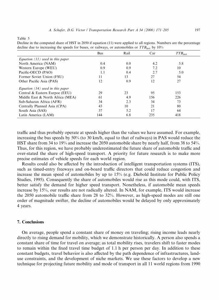
Fig. 14. The share of total mobility supplied by motorized transport in three world regions ± SAS, PAS, and MEA ± as

a function of income. Income statistics, expressed as GDP/cap in US$ (1980), are derived from the MEDS data base.

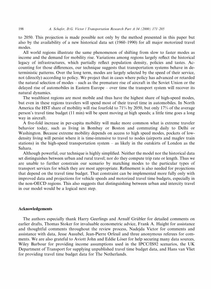
Fig. 15. PPP adjustments as a function of GNP/cap, expressed in US$ (1990), as derived from the IPCC IS92 scenario.

PPP adjustments, de®ned by the ratio of PPP (PWT5.6) and GNP (IPCC IS92), were used to transform the economic

growth rates from the IPCC scenario to growth rates that are appropriate for use with the PWT macroeconomic data

set, which is PPP-adjusted. Data points correspond to the world regions as de®ned in the IPCC IS92 scenarios.


1990). The MEDS and World Bank series are based on market exchange rates and not PPP-adjusted.

For illustrative purposes, Fig. 14 shows the consequence of using MEDS income data insteadof PWT for our projections in one cluster of regions ± SAS, PAS, MEA (Schafer, 1998). The PPPadjustment in the MEDS database results in a smooth transition, from SAS to PAS to MEA, ofall four modal split trajectories.

The prescribed growth rates used in this paper are derived from the IPCC/IS92 scenarios. Be-cause the IPCC growth rates apply to macroeconomic data that are based on market exchangerates, we have had to transform them for use with the PPP-adjusted PWT data set used in thispaper. This transformation was done as follows. First, the IPCC macroeconomic data for the baseyear (1990) and the IPCC projections were transformed into PPP data using a hyperbolic function.Fig. 15 shows the function, which was estimated using the relationship between GNP/cap for thenine IPCC regions and the world and the PPP data (from PWT) for those same regions in 1990.Second, we then estimated the growth rates that would be necessary in each region for income torise from the transformed IPCC base year to the transformed IPCC projected values for eachdecade, 1990 to 2050. The resulting ``transformed'' growth rates are reported in Table 2.

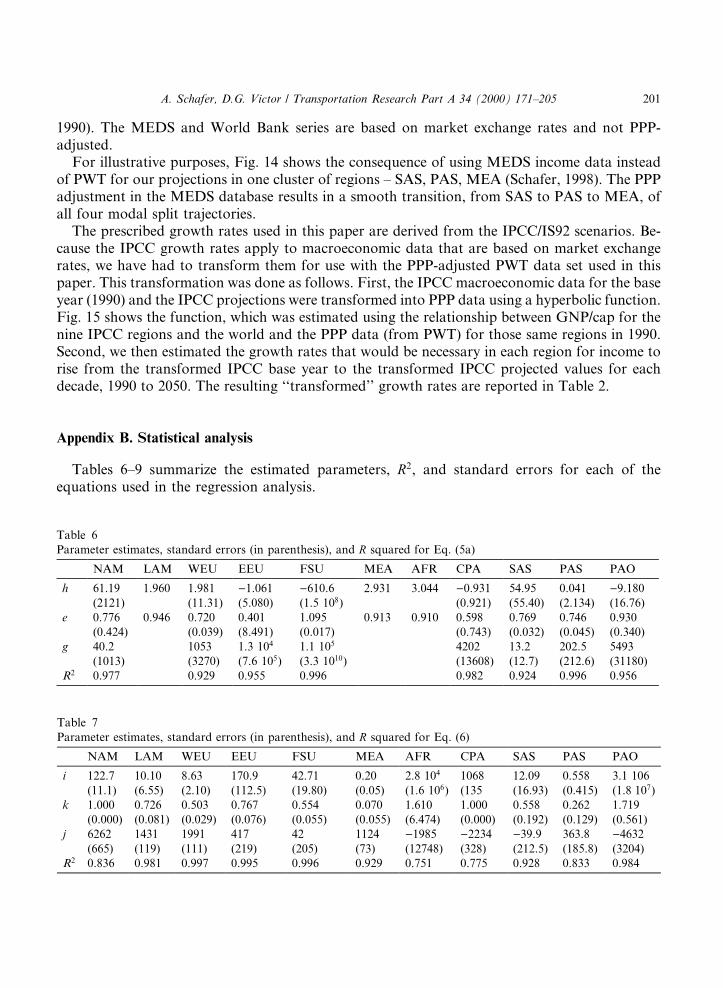
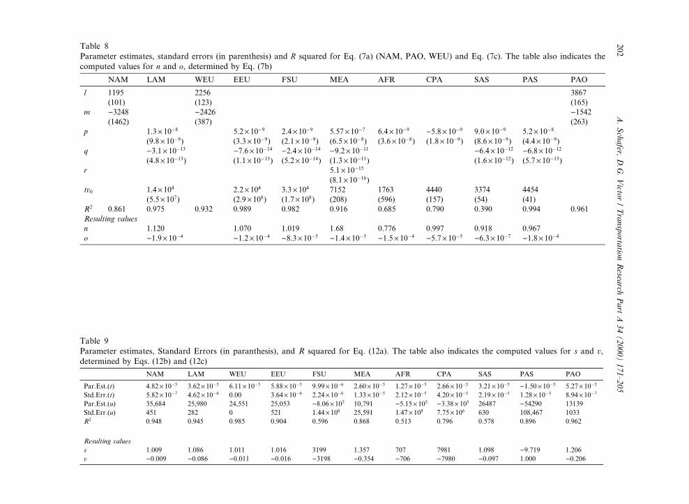
Appendix B. Statistical analysis

Tables 6±9 summarize the estimated parameters, R2, and standard errors for each of theequations used in the regression analysis.

Table 6

Parameter estimates, standard errors (in parenthesis), and R squared for Eq. (5a)

NAM LAM WEU EEU FSU MEA AFR CPA SAS PAS PAO

h 61.19

(2121)

1.960 1.981

(11.31)

)1.061

(5.080)

)610.6

(1.5 108)

2.931 3.044 )0.931

(0.921)

54.95

(55.40)

0.041

(2.134)

)9.180

(16.76)

e 0.776

(0.424)

0.946 0.720

(0.039)

0.401

(8.491)

1.095

(0.017)

0.913 0.910 0.598

(0.743)

0.769

(0.032)

0.746

(0.045)

0.930

(0.340)

g 40.2

(1013)

1053

(3270)

1.3 104

(7.6 105)

1.1 105

(3.3 1010)

4202

(13608)

13.2

(12.7)

202.5

(212.6)

5493

(31180)

R2 0.977 0.929 0.955 0.996 0.982 0.924 0.996 0.956

Table 7

Parameter estimates, standard errors (in parenthesis), and R squared for Eq. (6)


i 122.7

(11.1)

10.10

(6.55)

8.63

(2.10)

170.9

(112.5)

42.71

(19.80)

0.20

(0.05)

2.8 104

(1.6 106)

1068

(135

12.09

(16.93)

0.558

(0.415)

3.1 106

(1.8 107)

k 1.000

(0.000)

0.726

(0.081)

0.503

(0.029)

0.767

(0.076)

0.554

(0.055)

0.070

(0.055)

1.610

(6.474)

1.000

(0.000)

0.558

(0.192)

0.262

(0.129)

1.719

(0.561)

j 6262

(665)

1431

(119)

1991

(111)

417

(219)

42

(205)

1124

(73)

)1985

(12748)

)2234

(328)

)39.9

(212.5)

363.8

(185.8)

)4632

(3204)

R2 0.836 0.981 0.997 0.995 0.996 0.929 0.751 0.775 0.928 0.833 0.984


Table 8

Parameter estimates, standard errors (in parenthesis) and R squared for Eq. (7a) (NAM, PAO, WEU) and Eq. (7c). The table also indicates the

computed values for n and o, determined by Eq. (7b)


l 1195

(101)

2256

(123)

3867

(165)

m )3248

(1462)

)2426

(387)

)1542

(263)

p 1.3 ´ 10ÿ8

(9.8 ´ 10ÿ9)

5.2 ´ 10ÿ9

(3.3 ´ 10ÿ9)

2.4 ´ 10ÿ9

(2.1 ´ 10ÿ9)

5.57 ´ 10ÿ7

(6.5 ´ 10ÿ8)

6.4 ´ 10ÿ9

(3.6 ´ 10ÿ8)

)5.8 ´ 10ÿ9

(1.8 ´ 10ÿ9)

9.0 ´ 10ÿ9

(8.6 ´ 10ÿ9)

5.2 ´ 10ÿ8

(4.4 ´ 10ÿ9)

q )3.1 ´ 10ÿ13

(4.8 ´ 10ÿ13)

)7.6 ´ 10ÿ14

(1.1 ´ 10ÿ13)

)2.4 ´ 10ÿ14

(5.2 ´ 10ÿ14)

)9.2 ´ 10ÿ11

(1.3 ´ 10ÿ11)

)6.4 ´ 10ÿ12

(1.6 ´ 10ÿ12)

)6.8 ´ 10ÿ12

(5.7 ´ 10ÿ13)

r 5.1 ´ 10ÿ15

(8.1 ´ 10ÿ16)

tv0 1.4 ´ 104

(5.5 ´ 107)

2.2 ´ 104

(2.9 ´ 108)

3.3 ´ 104

(1.7 ´ 108)

7152

(208)

1763

(596)

4440

(157)

3374

(54)

4454

(41)

R2 0.861 0.975 0.932 0.989 0.982 0.916 0.685 0.790 0.390 0.994 0.961

Resulting values

n 1.120 1.070 1.019 1.68 0.776 0.997 0.918 0.967

o )1.9 ´ 10ÿ4 )1.2 ´ 10ÿ4 )8.3 ´ 10ÿ5 )1.4 ´ 10ÿ3 )1.5 ´ 10ÿ4 )5.7 ´ 10ÿ5 )6.3 ´ 10ÿ7 )1.8 ´ 10ÿ4

Table 9

Parameter estimates, Standard Errors (in paranthesis), and R squared for Eq. (12a). The table also indicates the computed values for s and v,

determined by Eqs. (12b) and (12c)


Par.Est.(t) 4.82 ´ 10ÿ5 3.62 ´ 10ÿ5 6.11 ´ 10ÿ5 5.88 ´ 10ÿ5 9.99 ´ 10ÿ6 2.60 ´ 10ÿ5 1.27 ´ 10ÿ5 2.66 ´ 10ÿ5 3.21 ´ 10ÿ5 )1.50 ´ 10ÿ5 5.27 ´ 10ÿ5

Std.Err.(t) 5.82 ´ 10ÿ7 4.62 ´ 10ÿ6 0.00 3.64 ´ 10ÿ6 2.24 ´ 10ÿ6 1.33 ´ 10ÿ5 2.12 ´ 10ÿ5 4.20 ´ 10ÿ5 2.19 ´ 10ÿ5 1.28 ´ 10ÿ5 8.94 ´ 10ÿ7

Par.Est.(u) 35,684 25,980 24,551 25,053 )8.06 ´ 105 10,791 )5.15 ´ 105 )3.38 ´ 105 26487 )54290 13139

Std.Err.(u) 451 282 0 521 1.44 ´ 108 25,591 1.47 ´ 108 7.75 ´ 106 630 108,467 1033

R2 0.948 0.945 0.985 0.904 0.596 0.868 0.513 0.796 0.578 0.896 0.962

Resulting values

s 1.009 1.086 1.011 1.016 3199 1.357 707 7981 1.098 )9.719 1.206

v )0.009 )0.086 )0.011 )0.016 )3198 )0.354 )706 )7980 )0.097 1.000 )0.206

20

2A

.S

cha

fer,D

.G.

Victo

r/

Tra

nsp

orta

tion

Resea

rchP

art

A3

4(

20

00

)1

71

±2

05

References

Airbus Industrie, 1998. Global Market Forecast ± GMF'98 1998±2017 (at: http://www.airbus.com/gmf98_2.html#De-

mand).

Alcamo, J., Bouwan, A., Edmonds, J., Gr�ubler, A., Morita, T., Sugandhy, A., 1995. An Evaluation of the IPCC IS92

Emission Scenarios. In: Houghton, J.T., Meira Filho, L.G., Bruce, J., Lee, H., Callander, B.A., Haites, E., Harris,

N., Maskell, K. (Eds.), Climate Change 1994. Cambridge University Press, Cambridge, UK, pp. 233±304.

Boeing, 1998. 1998 Current Market Outlook. Boeing, Seattle, WA (also at: http://www.boeing.com/cmo).

Button, K.J., 1993. Transport Economics. 2nd ed. Edward Elgar Publishing Company, Aldershot, England.

Bos, E., Vu, M.T., Levin, A., Bulatao, R.A., 1992. World Population Projections. Published for the World Bank,

Edition 1992 . The John Hopkins University Press Baltimore, MD.

Central Bureau voor de Statistiek (Ed.), 1978±1993. Statistical Yearbook of the Netherlands. The Hague, The

Netherlands.

Central Statistical O�ce (Ed.), 1970, 1980, 1990, 1993. Annual Abstract of Statistics of the UK. Her Majesty's

Stationary O�ce, London.

Covert, E. et al., 1992. Aeronautical Technologies for the Twenty-®rst Century. Aeronautics and Space Engineering

Board, National Research Council. National Academy Press, Washington, DC.

Davis, S.C., 1994. Transportation Energy Data Book, Edition 14. ORNL-6798 Oak Ridge National Laboratory, Oak

Ridge, TN.

Deaton, A., 1985. The demand for personal travel in developing countries: an empirical analysis. Transportation

Research Record 1037, 59±66.

Department of Transport National Travel Survey: 1985/86 Report ± Part 1: An Analysis of Personal Travel, 1988.

Department of Transport, London, UK.

Department of Transport National Travel Survey, 1989/91, (1993). Deparment of Transport, London, UK.

Department of Transport, 1994. Unpublished data of the 1985/865 and 1989/91 UK National Travel Surveys, London,

UK, (personal communication).

Deutsche Automobil Treuhand, 1994. Price of the average new car bought in Germany from 1970±1993. Personal

communication with Allgemeiner Deutscher Automobilclub (ADAC), Munich, Germany.

Deutsche Shell AG, 1995. Gipfel der Motorisierung in Sicht at: http://www.deutsche-shell.de/.

Deutsches Institut f�ur Wirtschaftsforschung. Verkehr in Zahlen, 1991, 1993, 1995. Bundesminister f�ur Verkehr, Bonn,

Germany.

Diebold Institute for Public Policy Studies. Transportation Infrastructures ± The Development of Intelligent

Transportation Systems, Praeger, Westport, CT.

Dienst f�ur Gesamtverkehrsfragen. Verkehrsverhalten in der Schweiz GFV-Report 6/91. 1992, 1989. GFV, Bern,

Switzerland.

Eads, G. C., Peake, S., Pariente-David, S., He�erson, M., 1998. Global transport and energy development: the scope

for change. Support paper, Working Group 1: Global Transport and Energy Development. 17th Congress of the

World Energy Council, Houston TX, 13±18 September 1998.

Eckerle, K., Hofer, P., Masuhr, K.P., 1992. Energiereport 2010 ± Die energiewirtschaftliche Entwicklung in

Deutschland, PROGNOS A.G. Sch�a�er±Poeschel Verlag, Stuttgart.

Environmental Protection Agency, 1990. Policy Options for Stabilizing Global Climate. Environmental Protection

Agency, Washington, DC.

EIDF (Equipment Ile De France), 1994. Les D�eplacements des Franciliens en 1991±1992. Enquete Globale de

Transport, 1994. Direction R�egionale de l'�Equipment, Paris.

Eurostat, 1994. Consumer expenditure survey data, Luxembourg (personal communication).

Federal Highway Administration, 1970±1991. Highway Statistics. US Department of Transportation, Washington,

DC.

Federal Highway Administration, 1992. Nationwide Personal Transportation Survey 1990. Public User Diskettes, US

Department of Transportation, Washington, DC.

FORS (Federal O�ce of Road Safety) 1988. Day-to-Day Travel in Australia 1985±86. Department of Transport

Communications Canberra Australia.


Gr�ubler, A., 1990. The Rise and Fall of Infrastructures. Physica-Verlag, Heidelberg.

Gr�ubler, A., Nakicenovic, N., 1991. The Evolution of Transport Systems: Past and Future. Research Report 91-8.

International Institute for Applied Systems Analysis, Laxenburg, Austria.

IIASA and WEC (International Institute for Applied Systems Analysis and World Energy Council), 1995. Global

Energy Perspectives to 2050 Beyond. Laxenburg, Austria; (IIASA), London UK (WEC).

ICAO (International Civil Aviation Organization) 1975±1991. Civil Aviation Statistics of the World. ICAO, Montreal,

Canada.

IRF (International Road Federation) (various years), World Road Statistics. Geneva, Washington, DC.

Jollands, N., 1995. Energy E�ciency ± How does New Zealand Shape up? ESCAP Energy News 5, vol. 12, no. 1.

United Nations, Environment and Natural Resources Management Division, Bangkok, Thailand, pp. 5±12.

Katiyar, R., Ohta, K., 1993. Concept of ÔDaily Travel TimeÕ (DTT) and its applicability to travel demand analysis.

Journal of the Faculty of Engineering, The University of Tokyo (B) 42 (2), 109±121.

Kloas, J., Kunert, U., Kuhfeld, H., 1993. Vergleichende Auswertungen von Haushaltsbefragungen zum Person-

ennahverkehr (KONTIV 1976, 1982, 1989). Gutachten im Auftrage des Bundesministers f�ur Verkehr. Deutsches

Institut f�ur Wirtschaftsforschung, Berlin.

Leggett, J., Pepper, W.J., Swart, R.J., 1992. Emissions scenarios for IPCC: an update. In: Houghton, J.T., Callander,

B.A., Varney, S.K. (Eds.), Climate Change 1992: The Supplementary Report to the IPCC Scienti®c Assessment.

Cambridge University Press, Cambridge, UK, pp. 69±95.

Levison, D.M., Kumar, A., 1994. The rational locator: why travel times have remained stable. Journal of the American

Planning Association 60 (3), 319±332.

Lutz, W. (Ed), 1996. The Future Population of the World: What Can We Assume Today. Earthscan, London.

Maddison, A., 1991. Dynamic Forces in Capitalist Development: A Long-run Comparative View: Oxford University

Press, Oxford.

Malasek, J., 1995. Transport problems in Warsaw ± possible solutions. In: Reconciling Transportation, Energy and

Environmental Issues: The Role of Public Transport. OECD, Paris, pp. 175±1981.

Marchetti, C., 1993. On Mobility. Final status report, contract no. 4672-92-03 ED ISP A. IIASA, Laxenburg, Austria.

Marchetti, C., 1994. Anthropological invariants in travel behavior. Technological Forecasting and Social Change 47,

75±88.

Martin, D.J., Shock, R.A.W., 1989. Energy Use and Energy E�ciency in UK Transport up to the Year 2010. Energy

E�ciency Series. Energy E�ciency O�ce, Department of Energy, London.

Metr~o, 1989. Pesquisa OD/87 ± S�intese das Informacß~oes. S~ao Paulo, Brazil.

Ministry of Infrastructure, no date. Trends in Person Trips in Urban Areas. Results of the 2nd Nationwide Urban

Transportation Survey (1987, 1992). O�ce of Urban Transportation, Tokyo.

Nakicenovic, N., 1988. Dynamics and replacement of US transport infrastructures. In: Ausubel, J.H., Herman, R.

(Eds.), Cities and their Vital Systems: Infrastructure Past, Present and Future. National Academy Press,

Washington, DC, pp. 175±221.

Nakicenovic, N., Gr�ubler, A., McDonald, A., 1998. Global Energy Perspectives. Cambridge University Press,

Cambridge.

Newman, P., Kenworthy, J., 1989. Cities and Automobile Dependence: An International Sourcebook. Avebury

Technical, Aldershot, UK.

Olszewski, P., Wong, Y.-D., Polak, J.W., Jones, P.M., 1994. Analysis of Travel Behavior in Singapore. Center for

Transportation Studies Report 94-02. Nanyang Technological University, Singapore.

Oppenheim, N., 1995. Urban Travel Demand Modeling, from Individual Choices to General Equilibrium. John Wiley

& Sons, New York.

Orfeuil, J.P., Salomon, I., 1993. Travel patterns of the Europeans in everyday life. In: Salomon, I., Bovy, P., Orfeuil,

J.P. (Eds.), A Billion Trips a Day ± Tradition and Transition in European Travel Patterns. Kluwer Academic

Publishers, Dordrecht, The Netherlands, pp. 33±50.

Riverson, J.D.N., Carapetis, S., 1991. Intermediate Means of Transport in Sub-Saharan Africa ± Its Potential for

Improving Rural Travel and Transport. World Bank Technical Paper Number 161. Technical Department Series.

The World Bank, Washington, DC.Roos, D., Altshuler, A., 1984. The Future of the Automobile ± The Report of MIT's International Automobile

Program. MIT Press, Cambridge.


Roth, G.J., Zahavi, Y., 1981. Travel time budgets in developing countries. Transportation Research A 15 (1), pp. 87±

95.

Schafer, A., 1998. The global demand for motorized mobility. Transportation Research A 32 (6), pp. 455±477.

Stab fur Gesamtverkehrsverhalten, 1986. Verkehrsverhalten in der Schweiz 1984. GVF-Bericht 2/86, Bern, Switzerland.

SSB (State Statistical Bureau of the PeopleÕs Republic of China) 1996. China Statistical Yearbook 1996. SSB, New

York..

Statistics Bureau 1972±1992. Japan Statistical Yearbook. Management and Coordination Agency, Tokyo.

Summers, R., Heston, A., Aten, B., Nuxoll, D., 1996. Penn World Tables, Mark 5.5 a. Center for International

Comparisons, University of Pennsylvania, Department of Economics, distributed through the US National Bureau

of Economic Research, Cambridge, MA.

Szalai, A., Converse, P.E., Feldheim, P., Scheuch, E.K., Stone, P.J., 1972. The Use of Time: Daily Activities of Urban

and Suburban Populations in 12 Countries. Mouton, The Hague.

United Nations, 1992. Long-Range World Population Projections: Two Centuries of Population Growth 1950±2150.

ST/ESA/SER.A/125, New York.

United Nations, 1993a. Annual Bulletin of Transport Statistics for Europe. United Nations, New York.

United Nations, 1993b. Macroeconomic Data System (MEDS). Long-Term Socio-Economic Perspectives Branch.

Department of Economic and Social Information and Policy Analysis, New York.

United Nations (Ed.), 1960±1992. Annual Bulletin of Transport Statistics for Europe. United Nations, New York.

US Department of Transportation, 1992. Nationwide Personal Transportation Survey 1990. Public User Diskettes, US

Department of Transportation, Washington, DC.

Vedantham, A., Oppenheimer, M., 1998. Long-term scenarios for aviation: demand and emissions of CO2 and NOx.

Energy Policy 26(8), pp. 625±641.

Vibe, N., 1993. V _are deglige Reiser ± Endringer i nordmenns reisevaner fra 1985 til 1992. Rapport 171/1993.

Transportokonomisk Institutt, Oslo, Norway.

Vliet, H., 1994. National Travel Survey Data. Ministry of Transport, Rotterdam, The Netherlands (personal

communication).

Walsh, M.P., 1993a. Transport sector analysis. In: Lazarus, M. et al. (Ed.), Towards a Fossil Free Energy Future, The

Next Energy Transition. Stockholm Environmental Institute, Boston, MA (for Greenpeace International), pp. 1±50.

Walsh, M.P., 1993b. Highway vehicle activity trends and their implications for global warming: the United States in an

international context. In: Greene, D.L., Santini, D.J. (Eds.), Transportation and Global Climate Change (American

Council for an Energy-E�cient Economy.) Washington DC and Berkeley, CA pp. 1±50.

World Bank, various years. World Development Report (and electronic versions). Oxford University Press, New York.

World Bank, Global Economic Prospects and the Developing Countries, 1996. The World Bank, Washington, DC.

Zahavi, Y., 1981. The UMOT±Urban Interactions. DOT-RSPA-DPB 10/7. US Department of Transportation,

Washington, DC.

Zahavi, Y., Talvitie, A., 1980. Regularities in travel time and money expenditures. Transportation Research Record

750, 13±19.


Date post:	05-May-2019
Category:	Documents
Upload:	hakhuong
View:	216 times
Download:	0 times

The future mobility of the world population -...

Documents