Research ArticleThe Fuzzy PI Controller for PMSMrsquos Speed to Track theStandard Model
Nguyen Vu Quynh
Electrical and Electronics Department Lac Hong University Bien Hoa Dong Nai Vietnam
Correspondence should be addressed to Nguyen Vu Quynh vuquynhlhueduvn
Received 4 April 2020 Revised 2 June 2020 Accepted 15 June 2020 Published 13 July 2020
Guest Editor Carlos Llopis-Albert
Copyright copy 2020Nguyen VuQuynh)is is an open access article distributed under the Creative Commons Attribution Licensewhich permits unrestricted use distribution and reproduction in any medium provided the original work is properly cited
)is paper proposes a fuzzy PI controller to control the speed of a permanent magnet synchronous motor (PMSM))e structureof the system includes the speed loop controller (SLC) and the current loop controller (CLC))e speed loop controller is the fuzzyPI and standard model (SM) )e CLC includes vector control and the space vector pulse width modulation (SVPWM) Itcompiles two closed-loop control systems for the PMSM )is research uses a very high-speed integrated circuit hardwaredescription language (VHDL) to implement the proposed algorithm and embed it into MatlabSimulink for simulation Based onthe PMSM parameter this article tests the controllerrsquos correctness with some of the load cases by changing the combined inertiaand viscous friction of rotor and load After success in simulation the system is tested again by experiment on the FPGA kit )esimulation and experiment results show that when the load changes the PMSM speed is still stable )e novelty of this research isthat it compares two kinds of controllers between simulation and experiment results
1 Introduction
)e PMSMs are commonly used in systems requiring highprecision such as the robot and mechanical processingHowever there are many uncertainties for example noiseexternal load and friction force)ey affect the performancequality of the system Many intelligent control techniquessuch as fuzzy neural network and genetic algorithm havebeen developed to cope with those problems [1ndash4] )eyhelped to control precisely the speed and position of themotor )e FPGA supplied a solution for the imple-mentation of the algorithm Especially FPGA has a pro-grammable hard-wired feature fast calculation ability lowpower consumption and higher density )ere were manytypes of research on intelligent controllers such as fuzzycontrol sliding fuzzy control artificial intelligence andadaptive control based on the FPGA platform to controlmultiaxis robots for improving precision in machining andassembly [5ndash9] )e fuzzy control method is an intelligentcontrol system with an inference mechanism from expertsrsquocontrol experience However obtaining fuzzy sets and op-timal membership functions are not easy To resolve this
problem the fuzzy knowledge base values were adjustedappropriately based on the feedback system parameter[10 11] )is research proposes a drive system to overcomethe slow response and tuning problems of the conventionalPI speed controllers without any mathematical calculations[12 13] However the aforementioned research studies donot check with the massive change of load )is researchapplied a fuzzy PI controller current controller andSVPWM for PMSM drive )e contents of the article in-clude firstly the mathematical model of PMSM SVPWMalgorithm vector control method and fuzzy PI controllerSecondly VHDL is used to program all systems Finally thearticle presents a simulation on MatlabSimulink and ex-periment on FPGA kit results
Figure 1 shows the block diagram of the proposed al-gorithm)e speed of the motor (ωr) is fed back to the speedloop controller to compare with the output of the standardmodel (SM) )e fuzzy PI controller generates the signal tominimize the error between rotor speed and SM )e ad-justment mechanism keeps the motor speed stable when theload changes )e three-phase stator currents (ia ib ic) androtor flux angle (θe) are fed back to the current controller to
HindawiMathematical Problems in EngineeringVolume 2020 Article ID 1698213 20 pageshttpsdoiorg10115520201698213
calculate the generated voltage vector for SVPWM )eSVPWM generated the electric current to control three-phase inverter for providing power to the motor
2 The Vector Controller Design for PMSM
21 e PMSM Mathematical Model
did
dt
1Ld
vd minusR
Ld
id +Lq
Ld
plowastωr lowast iq
diq
dt
1Lq
vq minusR
Lq
iq minusLd
Lq
plowastωr lowast id minusλlowastplowastωr
Lq
(1)
in which Lq and Ld are the inductances on q-axis and d-axisR isthe resistance of the stator windings iq and id are the currentson q-axis and d-axis Vq and Vd are the voltages on q-axis andd-axis λ is the permanent magnet flux linkage p is the numberof pole pairs and ωr is the rotational speed of the rotor
22 e Vector Controller )e current controller of thePMSM drive in Figure 1 is based on a vector control ap-proach )e current controller structure includes ClarkPark inverse Park and inverse Clark transformation twoPID controllers and sinecosine of flux angle )ree-phasecurrent is fed back through vector control enabling con-trolling current id asymp 0 which helps control the three-phasemotor similar to a DC motor )e torque of the PMSM iscontrolled via current on the q-axis (iq))e vector control isdescribed below
)e Clark transformation converts the stationary a-b-cframe (ia ib ic) to stationary α-β frame (iα iβ)
iα
iβ
⎡⎢⎢⎢⎢⎢⎣⎤⎥⎥⎥⎥⎥⎦
23
minus13
minus13
013
radicminus1
3
radic
⎡⎢⎢⎢⎢⎢⎢⎢⎢⎢⎢⎢⎢⎢⎢⎢⎢⎢⎢⎢⎢⎢⎢⎣
⎤⎥⎥⎥⎥⎥⎥⎥⎥⎥⎥⎥⎥⎥⎥⎥⎥⎥⎥⎥⎥⎥⎥⎦
ia
ib
ic
⎡⎢⎢⎢⎢⎢⎢⎢⎢⎢⎢⎢⎢⎢⎢⎢⎢⎢⎢⎢⎢⎢⎢⎢⎣
⎤⎥⎥⎥⎥⎥⎥⎥⎥⎥⎥⎥⎥⎥⎥⎥⎥⎥⎥⎥⎥⎥⎥⎥⎦ (2)
)e Park transformation converts the stationary α-βframe (iα iβ) to synchronously rotating d-q frame (id iq)
id
iq
⎡⎣ ⎤⎦ cos θe sin θe
minussin θe cos θe
1113890 1113891iα
iβ
⎡⎣ ⎤⎦ (3)
)e inverse Park transformation converts a rotatingreference d-q frame (vd vq to stationary α-β frame(vα vβ)
vα
vβ
⎡⎣ ⎤⎦ cos θe minussin θe
sin θe cos θe
1113890 1113891vd
vq
⎡⎣ ⎤⎦ (4)
)e inverse Clark transformation converts a stationaryα-β frame (vα vβ) to stationary a-b-c frame (vref1 vref2vref3)
vref1
vref2
vref3
⎡⎢⎢⎢⎢⎢⎢⎢⎢⎢⎢⎢⎢⎢⎢⎢⎢⎢⎢⎢⎢⎢⎢⎢⎢⎢⎣
⎤⎥⎥⎥⎥⎥⎥⎥⎥⎥⎥⎥⎥⎥⎥⎥⎥⎥⎥⎥⎥⎥⎥⎥⎥⎥⎦
1 0
minus12
3
radic
2
minus12
minus3
radic
2
⎡⎢⎢⎢⎢⎢⎢⎢⎢⎢⎢⎢⎢⎢⎢⎢⎢⎢⎢⎢⎢⎢⎢⎢⎢⎢⎢⎢⎢⎢⎢⎢⎢⎢⎢⎢⎢⎢⎢⎢⎢⎢⎢⎣
⎤⎥⎥⎥⎥⎥⎥⎥⎥⎥⎥⎥⎥⎥⎥⎥⎥⎥⎥⎥⎥⎥⎥⎥⎥⎥⎥⎥⎥⎥⎥⎥⎥⎥⎥⎥⎥⎥⎥⎥⎥⎥⎥⎦
vα
vβ
⎡⎢⎢⎢⎢⎢⎣⎤⎥⎥⎥⎥⎥⎦ (5)
Electromagnetic moment of the motor could be calcu-lated using the following formula
Te 15p λlowast iq + Ld minus Lq1113872 1113873id lowast iq1113960 1113961 asymp Kt lowast iq (6)
)emathematical equation of the motor under the load-bearing condition is
dωr
dt
1Jm Te minus Fωr minus Tm( 1113857
(7)
where Te is the motor torque Jm and F are the inertia andviscous friction of rotor and load Tm is the shaft mechanicaltorque and Kt is the torque constant
3 The SVPWM Algorithm Design
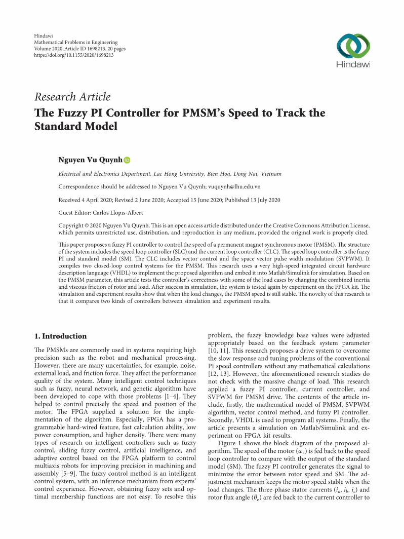
)e SVPWM is a control technique widely used in powerelectronic equipment control )e idea of the method is tocreate a continuous shift of the space vector equivalent of thevoltage vector of the inverter on the circle orbit (Figure 2)With the steady shift of the space vector on a circular orbit
SVPW
M
DCPower
PID
+
Parkndash1 Modified Clarkndash1
ndash
ndash+
PID a b c
d q
Current controller
Current loop
Park Clark
α β
α β
α β
α β
d q
a b c
Sinecosine of flux angle
A B C
PMSM
ωlowast
r
ilowastd = 0
ufilowastq
ωr
ωr
θe
ωm
uf ui
up
iq
id
iα
IGBT-base
inverter
iβ
vq
vd
vα
vβ
vref1
vref2
vref3
ia
ib
ic
Speed loop
+_
Fuzzy adjustment mechanism
Fuzzy inference
mechanism1 ndash Zndash1
e
de Fuzz
ifica
tion
Def
uzzi
ficat
ion
1 ndash Zndash1
Ki
Fuzzy knowledge base
Kp
+
+
Stan
dard
mod
el
Figure 1 )e simulation architecture of the fuzzy PI controller for PMSM drive
2 Mathematical Problems in Engineering
the higher harmonics are removed and the relationshipbetween the control signal and output voltage amplitudebecame linear In this article the SVPWM technique is usedto create a vector to control the inverter using IGBT powerswitches
)e phase-to-phase voltage and the phase-to-neutralvoltage of the motor
VAB
VBC
VCA
⎡⎢⎢⎢⎢⎢⎢⎢⎢⎢⎢⎢⎢⎢⎢⎢⎢⎢⎢⎢⎢⎢⎢⎢⎣
⎤⎥⎥⎥⎥⎥⎥⎥⎥⎥⎥⎥⎥⎥⎥⎥⎥⎥⎥⎥⎥⎥⎥⎥⎦ VDC
1 minus1 0
0 1 minus1
minus1 0 1
⎡⎢⎢⎢⎢⎢⎢⎢⎢⎢⎢⎢⎢⎢⎢⎢⎢⎢⎢⎢⎢⎢⎢⎢⎣
⎤⎥⎥⎥⎥⎥⎥⎥⎥⎥⎥⎥⎥⎥⎥⎥⎥⎥⎥⎥⎥⎥⎥⎥⎦
a
b
c
⎡⎢⎢⎢⎢⎢⎢⎢⎢⎢⎢⎢⎢⎢⎢⎢⎢⎢⎢⎢⎢⎢⎢⎢⎣
⎤⎥⎥⎥⎥⎥⎥⎥⎥⎥⎥⎥⎥⎥⎥⎥⎥⎥⎥⎥⎥⎥⎥⎥⎦
VAN
VBN
VCN
⎡⎢⎢⎢⎢⎢⎢⎢⎢⎢⎢⎢⎢⎢⎢⎢⎢⎢⎢⎢⎢⎢⎢⎢⎣
⎤⎥⎥⎥⎥⎥⎥⎥⎥⎥⎥⎥⎥⎥⎥⎥⎥⎥⎥⎥⎥⎥⎥⎥⎦13VDC
2 minus1 minus1
minus1 2 minus1
minus1 minus1 2
⎡⎢⎢⎢⎢⎢⎢⎢⎢⎢⎢⎢⎢⎢⎢⎢⎢⎢⎢⎢⎢⎢⎢⎢⎣
⎤⎥⎥⎥⎥⎥⎥⎥⎥⎥⎥⎥⎥⎥⎥⎥⎥⎥⎥⎥⎥⎥⎥⎥⎦
a
b
c
⎡⎢⎢⎢⎢⎢⎢⎢⎢⎢⎢⎢⎢⎢⎢⎢⎢⎢⎢⎢⎢⎢⎢⎢⎣
⎤⎥⎥⎥⎥⎥⎥⎥⎥⎥⎥⎥⎥⎥⎥⎥⎥⎥⎥⎥⎥⎥⎥⎥⎦
(8)
in which a b and c are switching vectors of IGBT powerelectronic switches
)ere are six power IGBTs in the voltage-source inverterWhen the upper switch is active the corresponding lowerswitches must be turned off)eremust be coordinated delaytime (dead band) between the opening and closing of twoswitches on the same phase
)e eight primary space vectors (V0 V1 V2
V3 V4 V5 V6 V7) are shown in Figure 2(a) )e outputvoltage (Vref) is located at one of the six sectors (S1 S2 S3 S4S5 S6) at any given time
Vref T1
TUx +
T2
TUx+1 +
T0 V0orV7( 1113857
T (9)
where xne 0 7 and T is half of the PWM periodT0 =TminusT1 minusT2 For example in the S3 sector the output
voltage can be calculated with V1 and V2 vectors(Figure 2(a))
V1 2VDC
3αrarr (10)
V2 VDC
3αrarr +
VDC3
radic βrarr
(11)
From equations (9)ndash(11) the output voltage and thevalue of T1 and T2 can be obtained
Vref T1lowastV1
T+
T2lowastV2
T
T1
T
2VDC
3αrarr
+T2
T
VDC
3αrarr +
VDC3
radic βrarr
1113888 1113889 asymp Vα αrarr
+ Vβ βrarr
T1 T 3Vα minus
3
radicVβ1113872 1113873
2VDC
T2
3
radicTlowastVβ
VDC
(12)
Similarly the values of T1 and T2 at the other sectorsshown in Table 1 with Tx Ty and Tz are
Tx
3
radicTlowastVβ
VDC
(13)
Ty T 3Vα +
3
radicVβ1113872 1113873
2VDC
(14)
Tz T minus3Vα +
3
radicVβ1113872 1113873
2VDC
(15)
V0V1
V2
V7
V3
V5 V6
V4
S1
S3
S2
Vref
T1
T2
S4
S6
S5
(ndash 23 0) ( 2
3 0)
(ndash 13
13
) ( 13
13
)
(ndash 13
13
ndash ) ( 13
13
ndash )
αα
β
(a)
CMP3
CMP2CMP1
PWM1
PWM2
PWM3
T1
T2
T02
T02
T T
V0 V1 V2 V7 V7 V2 V1 V0
(b)
Figure 2 (a) )e eight primary vectors and switching patterns (b) PWM at S3 Sector and its duty cycle
Mathematical Problems in Engineering 3
with the condition T1 +T2gtT T1 and T2 are modified asfollows
T1(cond) T1lowastT
T1 + T2 (16)
T2(cond) T2lowastT
T1 + T2 (17)
)e duty cycles (Taon Tbon Tcon) in Figure 2(b) cancalculated as follows
Taon T minus T1 minus T2
2
T0
2 (18)
Tbon Taon + T1 (19)
Tcon Tbon + T2 (20)
PWM1 PWM2 and PWM3 with the duty time at V1 andV2 and zero vector (V0 and V7) are T1 T2 and T0 respec-tively )e values of CMP1 CMP2 and CMP3 at each sectorare shown in Table 2 For quickly determining the sector (5)(inverse Clark transformation) is modified as follows
We can determine the sectors S1ndashS6 (Figure 3) accordingto the rule below
if Vref1 gt 0 then a 1 else a 0
if Vref2 gt 0 then b 1 else b 0
if Vref3 gt 0 then c 1 else c 0
(22)
)e sector of SVPWM is defined by this equationsector a+ 2b+ 4c From equations (13)ndash(15) and (21) wehave
Tx
Ty
Tz
⎡⎢⎢⎢⎢⎢⎢⎢⎢⎢⎢⎢⎢⎢⎢⎢⎢⎢⎢⎢⎢⎢⎢⎢⎣
⎤⎥⎥⎥⎥⎥⎥⎥⎥⎥⎥⎥⎥⎥⎥⎥⎥⎥⎥⎥⎥⎥⎥⎥⎦
3
radicT
VDC
vref1
minusvref3
minusvref2
⎡⎢⎢⎢⎢⎢⎢⎢⎢⎢⎢⎢⎢⎢⎢⎢⎢⎢⎢⎢⎢⎢⎢⎢⎢⎢⎣
⎤⎥⎥⎥⎥⎥⎥⎥⎥⎥⎥⎥⎥⎥⎥⎥⎥⎥⎥⎥⎥⎥⎥⎥⎥⎥⎦ (23)
)e implementation of SVPWM by VHDL can besummarized below
(i) From the value of Vref1 Vref2 and Vref3 we de-termined the sector as (22)
(ii) Calculate the value of Tx Ty and Tz from (23)(iii) Select T1 and T2 in Table 1(iv) Calculate the duty cycle (Taon Tbon and Tcon) from
equations (18)ndash(20)(v) Select comparative value (CMP1 CMP2 and CMP3)
at the duty cycles from Table 2
4 Standard Model (SM)
)e SM is the standard speed for PMSM )e output of theSM is increase and tangent to the set value at the input Tobuild the SM to meet the above requirements we used thetypical second-order system
ωm(s)
ωlowastr (s)
ω2n
s2 + 2lowast ηlowastωn lowast s + ω2n
(24)
where ωn and η are the natural frequency and damping ratiorespectively Using the bilinear transformation we obtainedthe discrete function in Z domain and difference equationωm zminus 1( 1113857
ωlowastr zminus1( )
a0 + a1zminus 1 + a2z
minus 2
1 + b1zminus1 + b2z
minus2
ωm(k) minusb1lowastωm(k minus 1) minus b2 lowastωm(k minus 2)
+ a0 lowastωlowastr (k) + a1lowastω
lowastr (k minus 1) + a2 lowastω
lowastr (k minus 2)
(25)
with coefficients a0 = 00077 a1 = 00153 a2 = 00077b1 =minus16496 and b2 = 06803
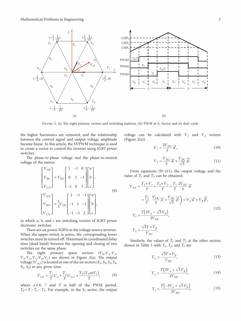
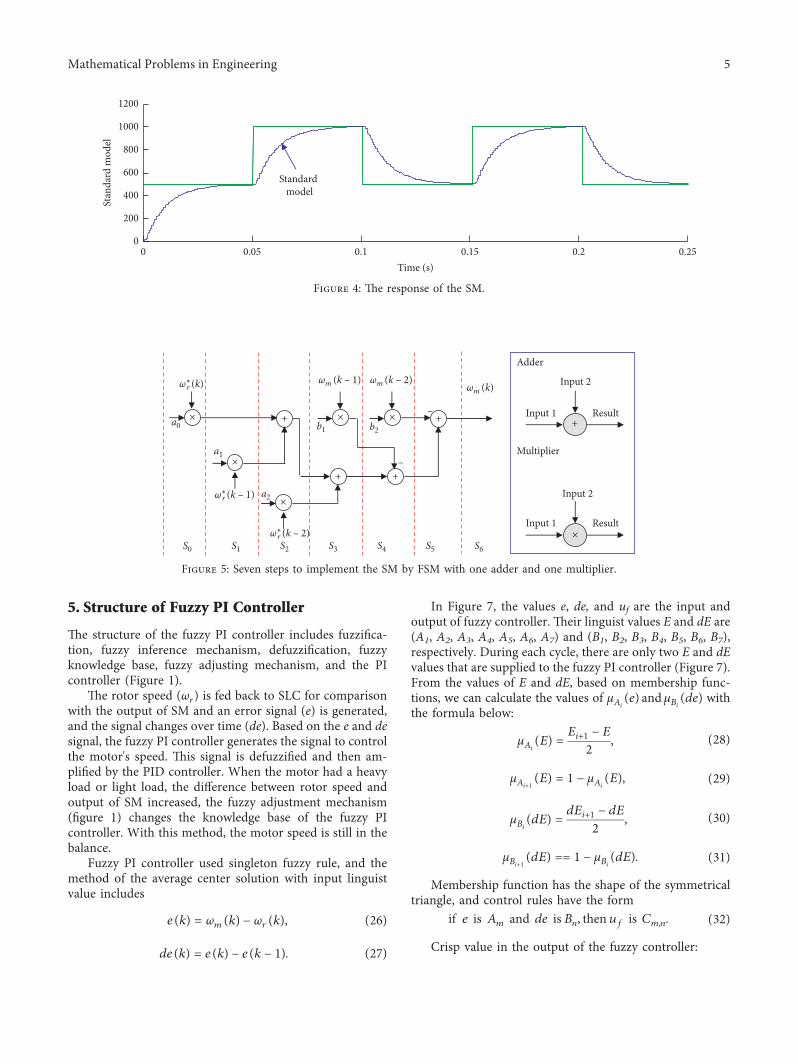
)e error between the output of SM and the rotor speed issupplied to the fuzzification and the fuzzy adjustment mech-anism function of the fuzzy PI controller Figure 4 shows theSM it does not change the rising time zero steady-state valueand overshoot when the system is running Figures 5 and 6show a finite state machine (FSM) and the VHDL code todescribe the SM respectively
Table 2 )e values of CMP1 CMP2 and CMP3 at each section
Section S 1 S 2 S 3 S 4 S 5 S 6
CMP1 Tb on Ta on Ta on Tc on Tc on Tb onCMP2 Ta on Tc on Tb on Tb on Ta on Tc onCMP3 Tc on Tb on Tc on Ta on Tb on Ta on
Degree0 60 120 180 240 300 0 60
S3 S1 S5 S4 S6 S2 S3
Vref1 Vref3 Vref2
Figure 3 )e voltage values supplying for the SVPWM
Table 1 Time value in each section
Value S 1 S 2 S 3 S 4 S 5 S 6
T 1 T z T y minusTz minusT x T x minusTyT 2 T y minusTx T x T z minusTy minusTz
4 Mathematical Problems in Engineering
5 Structure of Fuzzy PI Controller
)e structure of the fuzzy PI controller includes fuzzifica-tion fuzzy inference mechanism defuzzification fuzzyknowledge base fuzzy adjusting mechanism and the PIcontroller (Figure 1)
)e rotor speed (ωr) is fed back to SLC for comparisonwith the output of SM and an error signal (e) is generatedand the signal changes over time (de) Based on the e and designal the fuzzy PI controller generates the signal to controlthe motors speed )is signal is defuzzified and then am-plified by the PID controller When the motor had a heavyload or light load the difference between rotor speed andoutput of SM increased the fuzzy adjustment mechanism(figure 1) changes the knowledge base of the fuzzy PIcontroller With this method the motor speed is still in thebalance
Fuzzy PI controller used singleton fuzzy rule and themethod of the average center solution with input linguistvalue includes
e(k) ωm(k) minus ωr(k) (26)
de(k) e(k) minus e(k minus 1) (27)
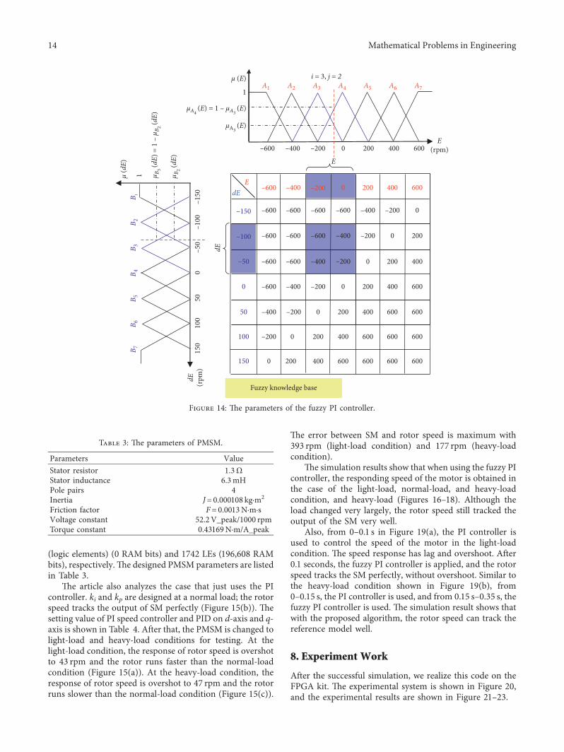
In Figure 7 the values e de and uf are the input andoutput of fuzzy controller )eir linguist values E and dE are(A1 A2 A3 A4 A5 A6 A7) and (B1 B2 B3 B4 B5 B6 B7)respectively During each cycle there are only two E and dEvalues that are supplied to the fuzzy PI controller (Figure 7)From the values of E and dE based on membership func-tions we can calculate the values of μAi
(e) and μBi(de) with
the formula below
μAi(E)
Ei+1 minus E
2 (28)
μAi+1(E) 1 minus μAi
(E) (29)
μBi(dE)
dEi+1 minus dE
2 (30)
μBi+1(dE) 1 minus μBi
(dE) (31)
Membership function has the shape of the symmetricaltriangle and control rules have the form
if e is Am and de is Bn then uf is Cmn (32)
Crisp value in the output of the fuzzy controller
Stan
dard
mod
el
Standard model
0
200
400
600
800
1000
1200
005 01 015 02 0250Time (s)
Figure 4 )e response of the SM
times
times
times
+
+
times times
+ndash
+ndash
S0
a2
a1
a0 b2b1
S1 S2 S3 S4 S5 S6
+
Input 2
Input 1 Result
times
Input 2
Input 1 Result
Adder
Multiplier
ωlowast
r (k)
ωlowast
r (k ndash 1)
ωm (k ndash 1) ωm (k ndash 2)ωm (k)
ωlowast
r (k ndash 2)
Figure 5 Seven steps to implement the SM by FSM with one adder and one multiplier
Mathematical Problems in Engineering 5
uf(E dE) 1113936
i+1ni1113936
j+1mjcmn μAn
(E)lowastμBm(dE)1113960 1113961
1113936i+1ni1113936
j+1mjμAn
(E)lowastμBm(dE)
Δ1113936
i+1ni1113936
j+1mjcmn lowastdnm
1113936i+1ni1113936
j+1mjdnm
1113944i+1
ni
1113944
j+1
mj
cmn lowastdnm
(33)
where dnm Δ μAn(E)lowastμBm
(dE) and cmn are adjustable pa-rameters in the adaptation mechanism Also it can beobtained by the equations (28)ndash(31) )erefore it isstraightforward to obtain 1113936
i+1ni1113936
j+1mjdnm 1 in (33)
)e purpose of the fuzzy adjustment mechanism is to createthe signal to adjust the fuzzy knowledge base of the fuzzy PIcontroller so that the error between the speed of the rotor and theoutput of the SM is the smallest We use the method of gradientdescent to determine the adaptive control law for the system
Definition of instantaneous value function
J(k + 1) 12[e(k + 1)]
212ωm(k + 1) minus ωr(k + 1)1113858 1113859
2
(34)
Parameter Cmn is determined by the variation of theinstantaneous value function
ΔCmn(k + 1) minusαzJ(k + 1)
zCmn(k) (35)
in which α shows the learning rate of the systemBy taking Laplace and bilinear transform of (7) we
obtained a discrete function in the Z domain of PMSM
ωr(k)
ilowastq (k)
Kt
F
1 minus e minus FTJm( )1113872 1113873zminus1
1 minus e minusFTJm( )zminus1 (36)
in which T is a sampling cycle and zminus1 is a stage of delaytime )e equation describes the relationship between ilowastqand uf
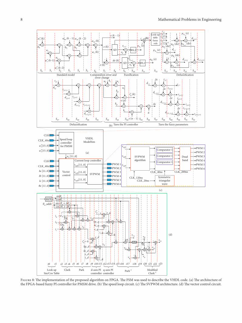
)e proposed algorithm has been embedded in one FPGAchip )e architecture of FPGA is shown in Figure 8 )eFSM sequential programming technique was used to de-scribe control algorithms )e internal circuit of the pro-posed algorithm includes one circuit of the SLC and onecircuit of the CLC
Figure 8(a) shows the implementation of FPGA forthe PMSM speed controller CLK and CLK_40ns are theinput clocks (50MHz and 25MHz) to supply all modules)e command speed and rotor speed (ωlowastr ωr) with 16 bitlength are the input of the SLC )e three-phase currents(ia ib ic) and rotor flux angle (θe) with 12 bit length arethe input of the CLC )e 6 PWMs are the output ofSVPWM
In Figure 8(b) there are 33 steps to carry out the fuzzy PIcontroller )e steps s0ndashs5 compute SM and the steps s6-s7calculate the rotor speed error with SM and error change)e steps s8ndashs11 compute the fuzzification )e step s12 looksup the fuzzy table to select four values of cmn based on i jobtained from s11 )e steps s13ndashs21 compute the defuzzi-fication function )e steps s22ndashs32 turn the PI and turn thefuzzy rule parameters
Figure 8(c) shows the design of SVPWM with 12 kHzfrequency and 12 μs dead band )e input of SVPWM isVref1 Vref2 and Vref3 with 12 bit length
Figure 8(d) computes the current vector controller andit takes 24 steps )e steps s0-s1 look up the table to take thevalue of sine and cosine functions )e steps s2ndashs8 calculatethe Clark and Park transformations )e PID controllerturns the current on d and q-axis from step s9ndashs14 )e stepss15ndashs23 calculate the inverse Park and modified inverse Clarktransformations
)e data type in vector control and SVPWM for PMSMis 12 bits )e data type is designed with 16 bit length for thefuzzy PI controller and SM Each clock pulse in the FPGA is40 ns to complete a command )ere are 33 steps (132 μs)and 24 steps (096 μs) to implement the SLC and the currentvector controller respectively It does not lose any perfor-mance because the operation time of fuzzy PI with 132 μs ismuch less than the sampling time of the speed controller(2 kHz)
Although the control algorithm of this research by usingthe fuzzy PI controller is quite complicated using the FSMdescription in step-by-step order reduced the execution timeof coding )e simulation was performed on MatlabSimulinkModelSim for adjusting and verifying the con-trollerrsquos parameters and checking the accuracy of the
dE
1
E(rpm)E
EdE
dE (rpm
)
micro (E)micro
(dE)
1
Fuzzy knowledge base
A7A1 A2 A3 A4 A5 A6
A7A1 A2 A3 A4 A5 A6
C17
B7
B1
B2
B3
B4
B5
B6
B 7B 1
B 2B 3
B 4B 5
B 6
C11 C12 C16C15C14C13
C27C21 C22 C26C25C24C23
C37C31 C32 C36C35C34C33
C47C41 C42 C46C45C44C43
C57C51 C52 C56C55C54C53
C67C61 C62 C66C65C64C63
C77C71 C72 C76C75C74C73
i = 3 j = 2
microA3 (E)microA4 (E) = 1 ndash microA3 (E)
micro B2 (d
E)
micro B3 (d
E) =
1 ndash
microB 2 (d
E)
Rule 1 E is A3 and dE is B2 then uf is c23Rule 2 E is A3 and dE is B3 then uf is c33Rule 3 E is A4 and dE is B2 then uf is c24Rule 4 E is A4 and dE is B3 then uf is c34
Figure 7 )e design of the fuzzy controller for PMSM drive
Mathematical Problems in Engineering 7
(d)
(b)
(c)
Speed loop controller for PMSM
VHDLModelSim
CLK
CLK_40n
ωlowast
r[150]
Vector control
Ia [110]
Ib [110]
Ic [110]
θe [110]
ωlowast
r[150]
ux [110]
vref1[110]
vref2[110]
vref3[110]
SVPWM
PWM 1PWM 2PWM 3PWM 4PWM 5PWM 6
CLK
CLK_40n
(a)
Current loop controller
Standard model Fuzzification
+
+
- SD
+-
+-
RS1
SD +-
RS1
ampi
j
Look-up table fuzzy rule
iampj
+1-
times
times
+
1- times
dij+1
di+1j
cji
cj i
cji
cji+1
cji+1
cji+1dij+1
di j
di j+1
cj+1i
di+1j
cji+1
di+1j+1
cj+1i+1
cj+1i
cj+1i
cj+1i
cj+1i+1
cj+1i+1
cj+1i+1
di j
cji
dij
di+1j+1
di+1 j
di+1 j+1
times
times +
times
times
times
+ + times
times
+
+
S6 S7 S8 S9 S10 S11 S12
Defuzzification Turn the PI controller
S13 S14 S15 S16
S17 S18 S19 S20 S21 S22 S23 S24
times
times
+ times
times +
times +
times +
times +
Defuzzification
S25 S26 S27 S28 S29 S30 S31 S32
timesa0a1
a2
ωlowast
r (k)
times
times
+
+
timesb1
timesb2
+-
+-
S0 S1 S2 S3 S4 S5
Computation error and error change
Turn the fuzzy parameters
SVPWM algorithm
Dead band
Symmetric triangular
wave
Comparator 1
Comparator 1
Comparator 1
PWM 1PWM 2PWM 3PWM 4PWM 5PWM 6
CLK_20nsCLK_120ns
CLK_40ns CLK_200ns
LUT
s1
ki_de_d
kp_d
i_d
e_d
i_d
ki_qe_q
kp_q
i_q
e_q
i_q
s2 s4s3 s5 s6 s8s7
ndash
s9 s10 s11 s13s12 s15
LS123
ndash
s16s14
ndash
s17 s18 s19 s20 s21 s22 s23
+
timestimes
+
cosθe
sinθe
+
+
times
timestimes
+
+
times
+vβ
vβ
+times
times
times
vα
iβiα
+
+
θe_addr
ndash
ndash
+
+
s0
ndash
+
d-axis PI controller
q-axis PI controller
Park-1ParkClarkLook upSinCos Table
ModifiedClark-1
3ndash1
31ndashtimes
times
times
times
+ times +
times +
2
cos (θe + ∆θc)sin (θe + ∆θc)
ωlowast
r (kndash1)
ωm (k ndash 1) ωm (k ndash 2)ωm (k)
ei+1
ei+1
microAi (e)
microBi (e)
microBj (de)
microBj (de)
microBj (de) microBj+1
(de)
microAi (e)
microAi+1 (e)
microAi (e)
ek
ek
e (k)
e (k)
e (n)
de (k)
e (k ndash 1)
e (n ndash 1)
ωr (k)
ωlowast
r (kndash2)
uf uiki
ki
kp
kp
ui
ilowastq (k)
α
∆c
∆c
∆c
∆c
∆c
ia
ib
ic
ilowastq
iq
id
vq
vd
vq
vrtimes
vrz
vry
vd
ilowastd = 0
vref1
vref2
vref3
Figure 8 )e implementation of the proposed algorithm on FPGA )e FSM was used to describe the VHDL code (a) )e architecture ofthe FPGA-based fuzzy PI controller for PMSM drive (b))e speed loop circuit (c))e SVPWM architecture (d))e vector control circuit
8 Mathematical Problems in Engineering
proposed algorithm )e ModelSim software was embeddedin MatlabSimulink for simulating the whole system )efeedback signals PMSMmodel and inverter are designed onSimulink After success in simulation the whole VHDL codeis downloaded to the FPGA board for testing again byexperiment
7 Simulation Work
)e simulation is demonstrated in this section to confirm theeffectiveness of the proposed architecture In simulationwork five steps are used to confirm the effectiveness of thesystem In the first step (Figure 9) the generation of
SVPWM function is firstly tested and its block diagramincludes inverse Clarke and inverse Park coordinatetransformation sincosine function and SVPWM(Figure 9(a)) In Figure 9(b) the EDA simulator link forModelSim executes the co-simulation using VHDL codewhich describes the function of the block diagram inFigure 9(a) )e switching frequency and dead band inSVPWM are designed with 16 kHz and 12 μs respectively)e input signal iq is set to a value varying from 01 to 04 id ischosen to be zero and the address (θe) is generated from 0 to360deg with increment by one )e PWM1ndashPWM6 outputs canbe generated through the computation in ModelSim FurtherPWM1 PWM3 and PWM5 are serially connected to the RC
SVPW
M
PWM1
PWM6
PWM2PWM3PWM4PWM5
a b c
d q
ModelSim
sincosfunction
iq
id = 0 α β
α βvα
vβ
vref1
vref2
vref3
Parkndash1Modified
Clarkndash1
θe
(a)
Saddle waveform of PWM
Convert
Convert
Convert
Convert
Convert
cmd_id
cmd_iq
Address
Address
-K-
Modelsim
Modelsim
PWM1
PWM6
PWM2
PWM3
PWM4
PWM5
Gain
Command
Id command
+
-s+
-s
+
-s CVS1
CVS2
CVS3
R1
R2
R3
C1
C2
C3
+- v
+- v
+- vVM3
PWM
VM1
VM2
0
(b)
SVPW
M
PWM 5PWM 1
PWM 302
04
06
08
005 01 015 02 0250Time (s)
(c)
Figure 9 )e simulation system for SVPWM generation (a) )e block diagram of step 1 (b) )e Simulink model of step 1 (c) )esimulation result of PWM with RC circuit connection (saddle waveform)
Mathematical Problems in Engineering 9
circuit (R 10Ω C 47) )e saddle waveform of PWMs isshown in Figure 9(c)
In step 2 the inverter and PMSM are added to step 1 Areal rotor flux angle replaces the address )e block diagramof this step is shown in Figure 10(a) and the Simulink modelis shown in Figure 10(c) )is step confirms the correctnessof SVPWM on PMSM again )e rotor speed is shown inFigure 10(b) and it follows the value of iq at the input
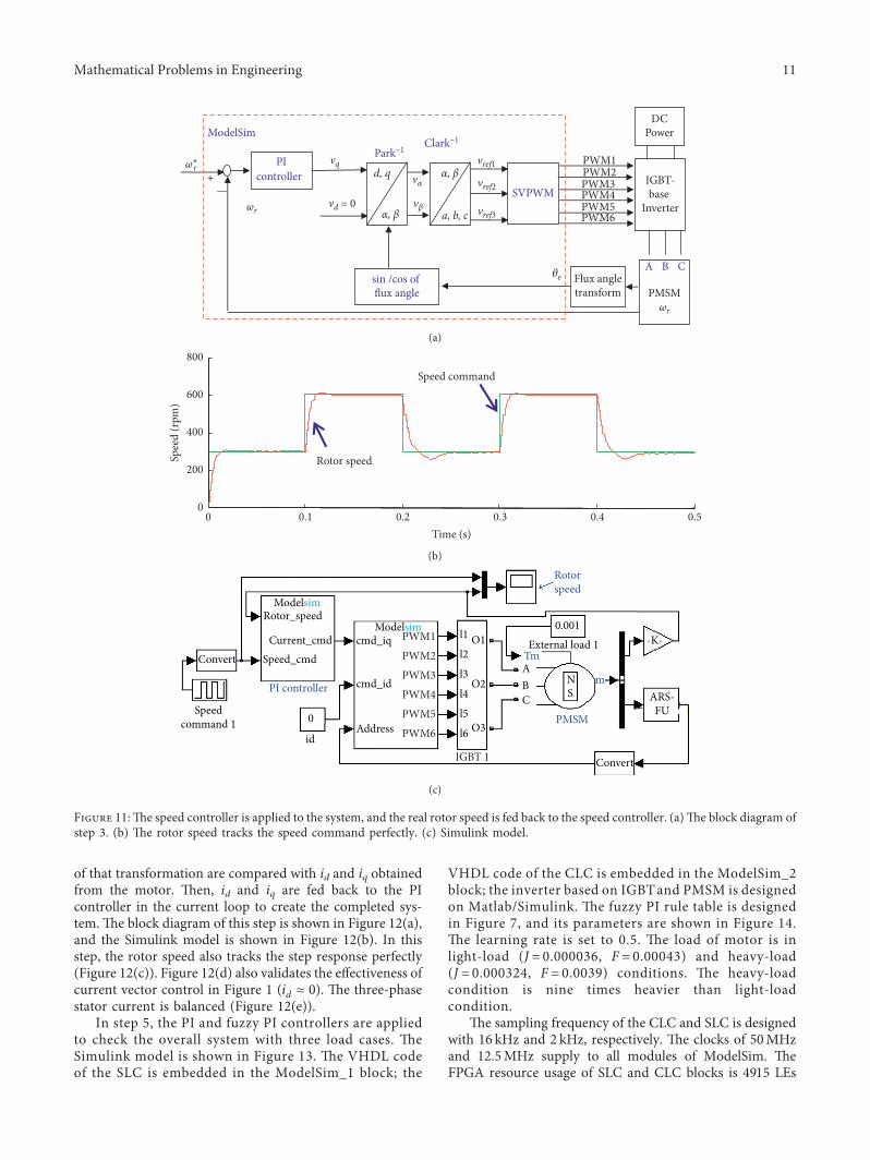
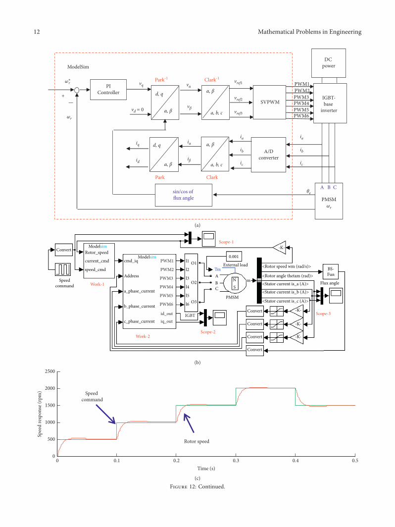
In step 3 the PI speed controller is applied to the systemand the real rotor speed is fed back to the speed controller)e block diagram of this step is shown in Figure 11(a) andthe Simulink model is shown in Figure 11(c) In this step wecan check the speed response of PMSM)e rotor speed canfollow well the step response at the input (Figure 11(b))
In step 4 the three-phase stator currents are fed back andapplied through Clack and Pack transformation )e results
SVPWM
DCPower
PWM1
PWM6
PWM2PWM3PWM4PWM5a b c
d q
ModelSim
sincos of Flux angle
Flux angleTransform PMSM
IGBT-base
Inverter
A B C
iq
id = 0
α β
α β
θe
vα
vβ
vref1
vref2
vref3
Parkndash1 Clarkndash1
(a)
Spee
d (R
PM)
0
250
500
750
1000
01 02 03 04 050Time (s)
(b)
Convert
Convert
Speedcommand
cmd_iq
cmd_id
Address
ABC
NS
0001
External loadTm
-K-Modelsim
PWM1
PWM6
PWM2
PWM3
PWM4
PWM5
IGBT
0 m
id ABS-FU
l1
l2
l3
l4
l5
l6
O1
O2
O3
ModelSim
PMSM
Rotorspeed
(c)
Figure 10 Confirmation of the correctness of SVPWM on the PMSM model again (a) )e block diagram of step 2 (b) )e rotor speedresponse (c) )e Simulink model
10 Mathematical Problems in Engineering
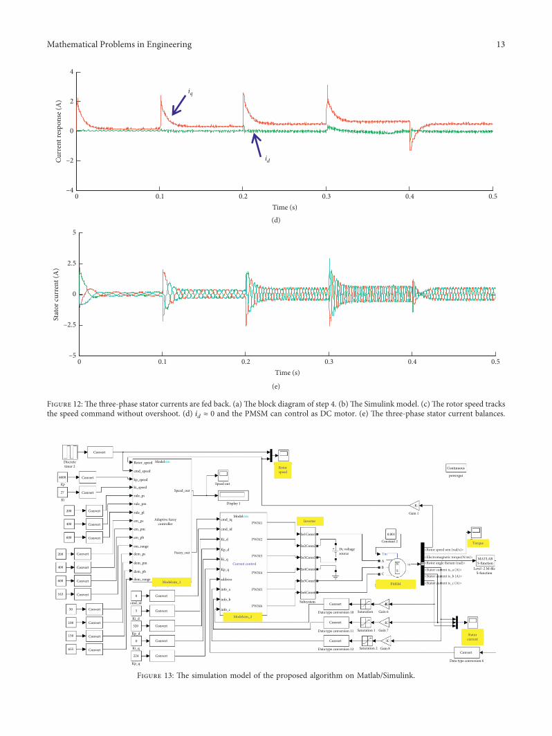
of that transformation are compared with id and iq obtainedfrom the motor )en id and iq are fed back to the PIcontroller in the current loop to create the completed sys-tem)e block diagram of this step is shown in Figure 12(a)and the Simulink model is shown in Figure 12(b) In thisstep the rotor speed also tracks the step response perfectly(Figure 12(c)) Figure 12(d) also validates the effectiveness ofcurrent vector control in Figure 1 (id asymp 0) )e three-phasestator current is balanced (Figure 12(e))
In step 5 the PI and fuzzy PI controllers are appliedto check the overall system with three load cases )eSimulink model is shown in Figure 13 )e VHDL codeof the SLC is embedded in the ModelSim_1 block the
VHDL code of the CLC is embedded in the ModelSim_2block the inverter based on IGBTand PMSM is designedon MatlabSimulink )e fuzzy PI rule table is designedin Figure 7 and its parameters are shown in Figure 14)e learning rate is set to 05 )e load of motor is inlight-load (J 0000036 F 000043) and heavy-load(J 0000324 F 00039) conditions )e heavy-loadcondition is nine times heavier than light-loadcondition
)e sampling frequency of the CLC and SLC is designedwith 16 kHz and 2 kHz respectively )e clocks of 50MHzand 125MHz supply to all modules of ModelSim )eFPGA resource usage of SLC and CLC blocks is 4915 LEs
SVPWM
DCPower
IGBT-base
Inverter
PWM1
PWM6
PWM2PWM3PWM4PWM5
ModelSim
sin cos of flux angle
Flux angletransform PMSM
ωr
+mdash
PIcontroller
a b c
d q α β
α β
θe
vref1
vref2
vref3
Parkndash1 Clarkndash1
ωlowast
r
ωr
vα
vβ
vq
vd = 0
A B C
(a)
Spee
d (r
pm)
Speed command
Rotor speed
0
200
400
600
800
01 02 03 04 050Time (s)
(b)
Rotor_speed
Current_cmdSpeed_cmdConvert
Convert
Speedcommand 1
-K-
Modelsim
cmd_iq
cmd_id
Address
ModelsimPWM1
PWM6
PWM2PWM3PWM4PWM5
IGBT 1
ABC
NS
0001External load 1
Tm
m
0
id
ARS-FU
l1
l2
l3
l4
l5
l6
O1
O2
O3
PI controller
PMSM
Rotorspeed
(c)
Figure 11)e speed controller is applied to the system and the real rotor speed is fed back to the speed controller (a))e block diagram ofstep 3 (b) )e rotor speed tracks the speed command perfectly (c) Simulink model
Figure 13 )e simulation model of the proposed algorithm on MatlabSimulink
Curr
ent r
espo
nse (
A)
iq
id
ndash4
ndash2
0
2
4
01 02 03 04 050Time (s)
(d)
Stat
or cu
rren
t (A
)
ndash5
ndash25
0
25
5
01 02 03 04 050Time (s)
(e)
Figure 12 )e three-phase stator currents are fed back (a))e block diagram of step 4 (b))e Simulink model (c))e rotor speed tracksthe speed command without overshoot (d) id asymp 0 and the PMSM can control as DC motor (e) )e three-phase stator current balances
Mathematical Problems in Engineering 13
(logic elements) (0 RAM bits) and 1742 LEs (196608 RAMbits) respectively)e designed PMSM parameters are listedin Table 3
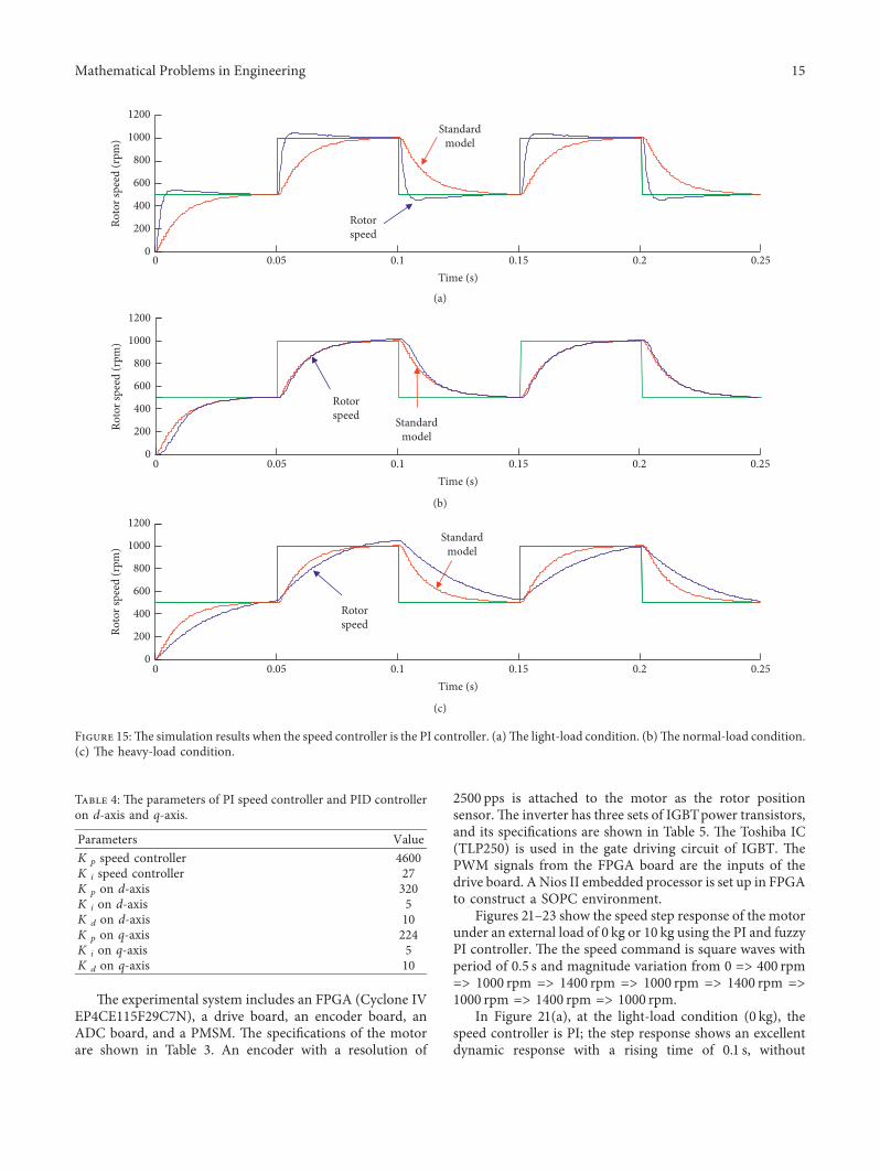
)e article also analyzes the case that just uses the PIcontroller ki and kp are designed at a normal load the rotorspeed tracks the output of SM perfectly (Figure 15(b)) )esetting value of PI speed controller and PID on d-axis and q-axis is shown in Table 4 After that the PMSM is changed tolight-load and heavy-load conditions for testing At thelight-load condition the response of rotor speed is overshotto 43 rpm and the rotor runs faster than the normal-loadcondition (Figure 15(a)) At the heavy-load condition theresponse of rotor speed is overshot to 47 rpm and the rotorruns slower than the normal-load condition (Figure 15(c))
)e error between SM and rotor speed is maximum with393 rpm (light-load condition) and 177 rpm (heavy-loadcondition)
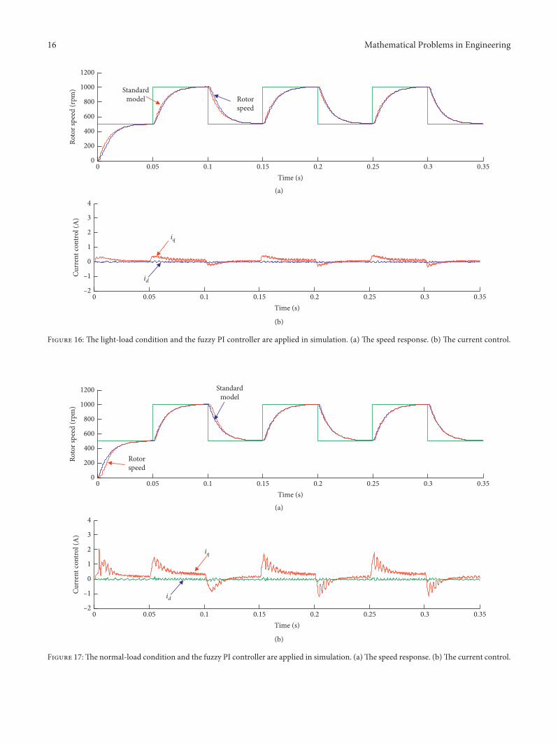
)e simulation results show that when using the fuzzy PIcontroller the responding speed of the motor is obtained inthe case of the light-load normal-load and heavy-loadcondition and heavy-load (Figures 16ndash18) Although theload changed very largely the rotor speed still tracked theoutput of the SM very well
Also from 0ndash01 s in Figure 19(a) the PI controller isused to control the speed of the motor in the light-loadcondition )e speed response has lag and overshoot After01 seconds the fuzzy PI controller is applied and the rotorspeed tracks the SM perfectly without overshoot Similar tothe heavy-load condition shown in Figure 19(b) from0ndash015 s the PI controller is used and from 015 sndash035 s thefuzzy PI controller is used )e simulation result shows thatwith the proposed algorithm the rotor speed can track thereference model well
8 Experiment Work
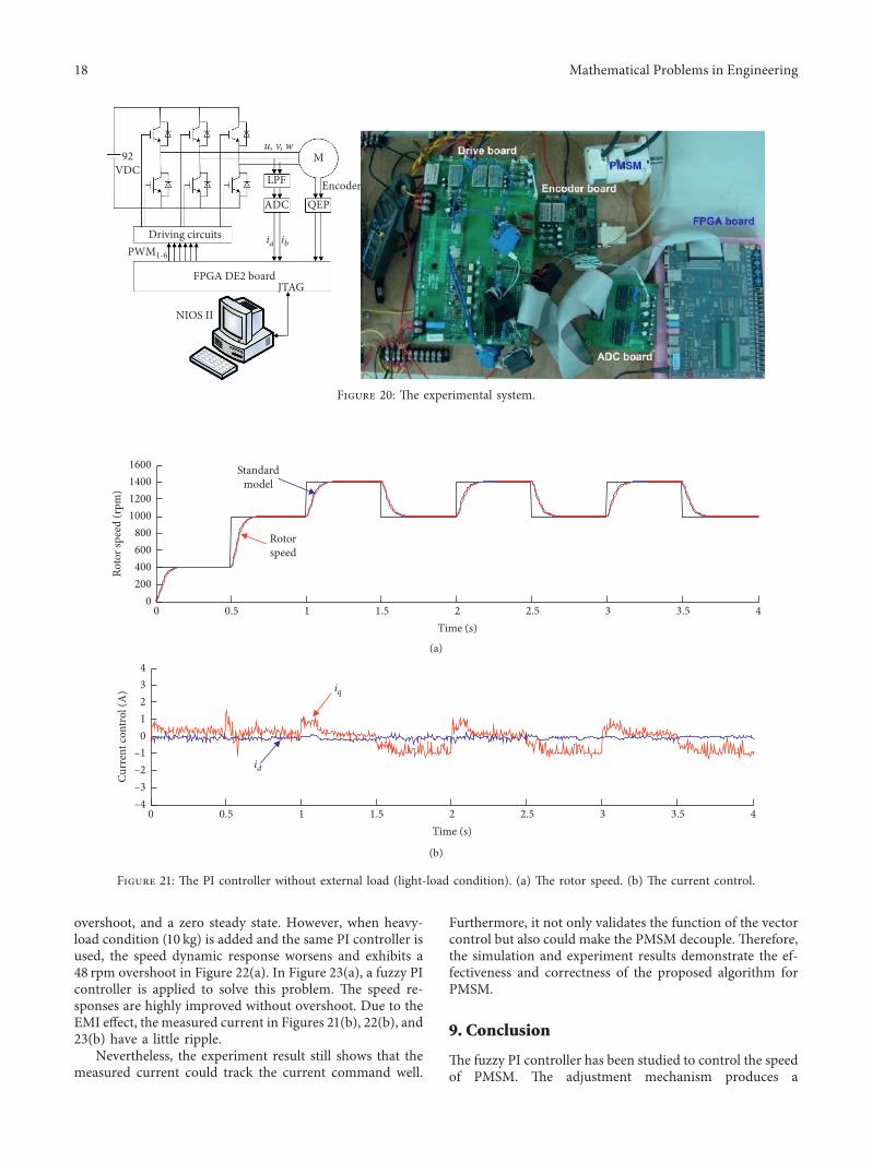
After the successful simulation we realize this code on theFPGA kit )e experimental system is shown in Figure 20and the experimental results are shown in Figure 21ndash23
dE
E
E
dE
1
Fuzzy knowledge base
ndash600 ndash400 ndash200 0 200
ndash600
ndash400
ndash200
0
200
400
ndash150
ndash100
ndash50
0
50
100
150
600
0
200
400
600
600
600
600
ndash600
ndash600
ndash600
ndash600
ndash400
ndash200
0
ndash600
ndash600
ndash600
ndash400
ndash200
0
200
400
ndash200
0
200
400
600
600
600
ndash400
ndash200
0
200
400
600
600600
ndash600
ndash600
ndash400
ndash200
0
200
400
i = 3 j = 2
1
0ndash600 400200ndash400 ndash200 600
015
0ndash1
5010
050
ndash100
ndash50
dE (rpm
)
micro (E)
micro (d
E)
A7A1 A2 A3 A4 A5 A6
B 7B 1
B 2B 3
B 4B 5
B 6microA3 (E)
microA4 (E) = 1 ndash microA3 (E)
micro B2 (d
E)
micro B3 (d
E) =
1 ndash
microB 2 (d
E)
E(rpm)
Figure 14 )e parameters of the fuzzy PI controller
Friction factor F 00013NmiddotmmiddotsVoltage constant 522V_peak1000 rpmTorque constant 043169NmiddotmA_peak
14 Mathematical Problems in Engineering
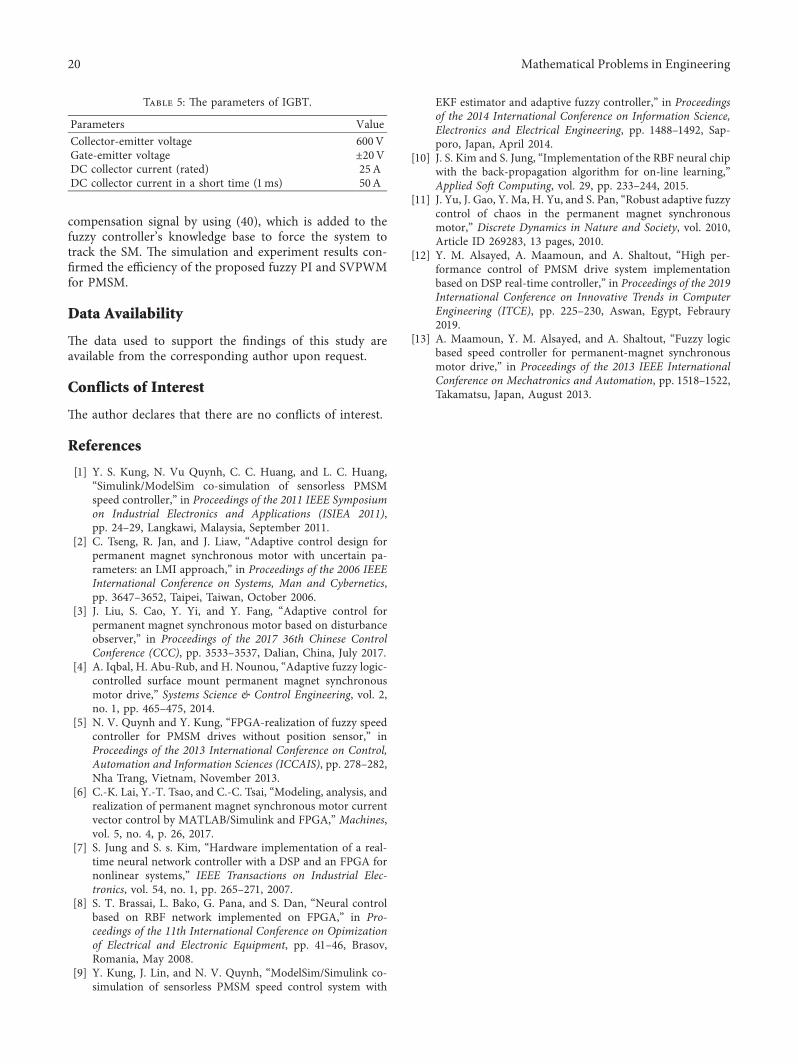
)e experimental system includes an FPGA (Cyclone IVEP4CE115F29C7N) a drive board an encoder board anADC board and a PMSM )e specifications of the motorare shown in Table 3 An encoder with a resolution of
2500 pps is attached to the motor as the rotor positionsensor)e inverter has three sets of IGBTpower transistorsand its specifications are shown in Table 5 )e Toshiba IC(TLP250) is used in the gate driving circuit of IGBT )ePWM signals from the FPGA board are the inputs of thedrive board ANios II embedded processor is set up in FPGAto construct a SOPC environment
Figures 21ndash23 show the speed step response of the motorunder an external load of 0 kg or 10 kg using the PI and fuzzyPI controller )e the speed command is square waves withperiod of 05 s and magnitude variation from 0 =gt 400 rpm=gt 1000 rpm =gt 1400 rpm =gt 1000 rpm =gt 1400 rpm =gt1000 rpm =gt 1400 rpm =gt 1000 rpm
In Figure 21(a) at the light-load condition (0 kg) thespeed controller is PI the step response shows an excellentdynamic response with a rising time of 01 s without
Standardmodel
Rotorspeed
Roto
r spe
ed (r
pm)
005 01 015 020 025Time (s)
0
200
400
600
800
1000
1200
(a)
Standardmodel
Rotorspeed
Roto
r spe
ed (r
pm)
005 01 015 020 025Time (s)
0
200
400
600
800
1000
1200
(b)
Standardmodel
RotorspeedRo
tor s
peed
(rpm
)
005 01 015 020 025Time (s)
0
200
400
600
800
1000
1200
(c)
Figure 15)e simulation results when the speed controller is the PI controller (a))e light-load condition (b))e normal-load condition(c) )e heavy-load condition
Table 4 )e parameters of PI speed controller and PID controlleron d-axis and q-axis
Parameters ValueK p speed controller 4600K i speed controller 27K p on d-axis 320K i on d-axis 5K d on d-axis 10K p on q-axis 224K i on q-axis 5K d on q-axis 10
Mathematical Problems in Engineering 15
Standardmodel
Rotorspeed
Roto
r spe
ed (r
pm)
005 01 015 02 025 03 0350Time (s)
0
200
400
600
800
1000
1200
(a)
005 01 015 02 025 03 0350Time (s)
iq
id
Curr
ent c
ontro
l (A
)
ndash2
ndash1
0
1
2
3
4
(b)
Figure 17)e normal-load condition and the fuzzy PI controller are applied in simulation (a))e speed response (b))e current control
Standardmodel Rotor
speed
Roto
r spe
ed (r
pm)
005 01 015 02 025 03 0350Time (s)
0
200
400
600
800
1000
1200
(a)
iq
id
Curr
ent c
ontro
l (A
)
005 01 015 02 025 03 0350Time (s)
ndash2
ndash1
0
1
2
3
4
(b)
Figure 16 )e light-load condition and the fuzzy PI controller are applied in simulation (a) )e speed response (b) )e current control
16 Mathematical Problems in Engineering
Rotor speed
Standardmodel
Fuzzy PIPI
Roto
r spe
ed (r
pm)
005 01 015 02 025 03 0350Time (s)
0
200
400
600
800
1000
1200
(a)
Fuzzy PIPI
Rotor speed
Standardmodel
Roto
r spe
ed (r
pm)
005 01 015 02 025 03 0350Time (s)
0
200
400
600
800
1000
1200
(b)
Figure 19 )e PI and fuzzy PI controllers are applied in simulation (a) )e light-load condition (b) )e heavy-load condition
Standard model
Rotorspeed
Roto
r spe
ed (r
pm)
005 01 015 02 025 03 0350Time (s)
0
200
400
600
800
1000
1200
(a)
iq
id
Curr
ent c
ontro
l (A
)
005 01 015 02 025 03 0350Time (s)
ndash2
ndash1
0
1
2
3
4
(b)
Figure 18 )e heavy-load condition and the fuzzy PI controller are applied in simulation (a) )e speed response (b) )e current control
Mathematical Problems in Engineering 17
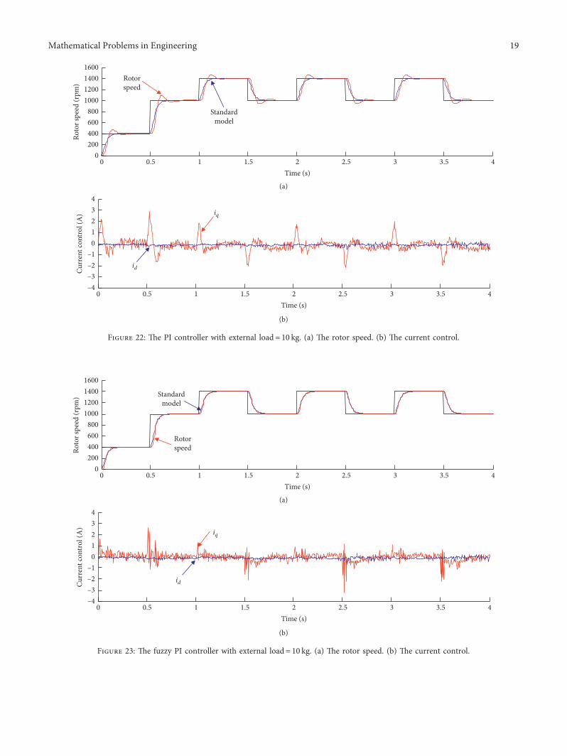
overshoot and a zero steady state However when heavy-load condition (10 kg) is added and the same PI controller isused the speed dynamic response worsens and exhibits a48 rpm overshoot in Figure 22(a) In Figure 23(a) a fuzzy PIcontroller is applied to solve this problem )e speed re-sponses are highly improved without overshoot Due to theEMI effect the measured current in Figures 21(b) 22(b) and23(b) have a little ripple
Nevertheless the experiment result still shows that themeasured current could track the current command well
Furthermore it not only validates the function of the vectorcontrol but also could make the PMSM decouple )ereforethe simulation and experiment results demonstrate the ef-fectiveness and correctness of the proposed algorithm forPMSM
9 Conclusion
)e fuzzy PI controller has been studied to control the speedof PMSM )e adjustment mechanism produces a
Roto
r spe
ed (r
pm)
0200400600800
1000120014001600
05 1 15 2 25 3 35 40Time (s)
Standardmodel
Rotorspeed
(a)
iq
id
Curr
ent c
ontro
l (A
)
05 1 15 2 25 3 35 40Time (s)
ndash4ndash3ndash2ndash1
01234
(b)
Figure 21 )e PI controller without external load (light-load condition) (a) )e rotor speed (b) )e current control
92VDC
u v w
LPF
ADC QEP
M
Encoder
Driving circuits
JTAGFPGA DE2 board
NIOS II
PWM1-6
ia ib
Figure 20 )e experimental system
18 Mathematical Problems in Engineering
Standardmodel
RotorspeedRo
tor s
peed
(rpm
)
0200400600800
1000120014001600
05 1 15 2 25 3 35 40Time (s)
(a)
iq
idCurr
ent c
ontro
l (A
)
ndash4ndash3ndash2ndash1
01234
05 1 15 2 25 3 35 40Time (s)
(b)
Figure 23 )e fuzzy PI controller with external load 10 kg (a) )e rotor speed (b) )e current control
Standardmodel
Rotorspeed
Roto
r spe
ed (r
pm)
0200400600800
1000120014001600
05 1 15 2 25 3 35 40Time (s)
(a)
iq
idCurr
ent c
ontro
l (A
)
ndash4ndash3ndash2ndash1
01234
05 1 15 2 25 3 35 40Time (s)
(b)
Figure 22 )e PI controller with external load 10 kg (a) )e rotor speed (b) )e current control
Mathematical Problems in Engineering 19
compensation signal by using (40) which is added to thefuzzy controllerrsquos knowledge base to force the system totrack the SM )e simulation and experiment results con-firmed the efficiency of the proposed fuzzy PI and SVPWMfor PMSM
Data Availability
)e data used to support the findings of this study areavailable from the corresponding author upon request
Conflicts of Interest
)e author declares that there are no conflicts of interest
References
[1] Y S Kung N Vu Quynh C C Huang and L C HuangldquoSimulinkModelSim co-simulation of sensorless PMSMspeed controllerrdquo in Proceedings of the 2011 IEEE Symposiumon Industrial Electronics and Applications (ISIEA 2011)pp 24ndash29 Langkawi Malaysia September 2011
[2] C Tseng R Jan and J Liaw ldquoAdaptive control design forpermanent magnet synchronous motor with uncertain pa-rameters an LMI approachrdquo in Proceedings of the 2006 IEEEInternational Conference on Systems Man and Cyberneticspp 3647ndash3652 Taipei Taiwan October 2006
[3] J Liu S Cao Y Yi and Y Fang ldquoAdaptive control forpermanent magnet synchronous motor based on disturbanceobserverrdquo in Proceedings of the 2017 36th Chinese ControlConference (CCC) pp 3533ndash3537 Dalian China July 2017
[4] A Iqbal H Abu-Rub and H Nounou ldquoAdaptive fuzzy logic-controlled surface mount permanent magnet synchronousmotor driverdquo Systems Science amp Control Engineering vol 2no 1 pp 465ndash475 2014
[5] N V Quynh and Y Kung ldquoFPGA-realization of fuzzy speedcontroller for PMSM drives without position sensorrdquo inProceedings of the 2013 International Conference on ControlAutomation and Information Sciences (ICCAIS) pp 278ndash282Nha Trang Vietnam November 2013
[6] C-K Lai Y-T Tsao and C-C Tsai ldquoModeling analysis andrealization of permanent magnet synchronous motor currentvector control by MATLABSimulink and FPGArdquo Machinesvol 5 no 4 p 26 2017
[7] S Jung and S s Kim ldquoHardware implementation of a real-time neural network controller with a DSP and an FPGA fornonlinear systemsrdquo IEEE Transactions on Industrial Elec-tronics vol 54 no 1 pp 265ndash271 2007
[8] S T Brassai L Bako G Pana and S Dan ldquoNeural controlbased on RBF network implemented on FPGArdquo in Pro-ceedings of the 11th International Conference on Opimizationof Electrical and Electronic Equipment pp 41ndash46 BrasovRomania May 2008
[9] Y Kung J Lin and N V Quynh ldquoModelSimSimulink co-simulation of sensorless PMSM speed control system with
EKF estimator and adaptive fuzzy controllerrdquo in Proceedingsof the 2014 International Conference on Information ScienceElectronics and Electrical Engineering pp 1488ndash1492 Sap-poro Japan April 2014
[10] J S Kim and S Jung ldquoImplementation of the RBF neural chipwith the back-propagation algorithm for on-line learningrdquoApplied Soft Computing vol 29 pp 233ndash244 2015
[11] J Yu J Gao Y Ma H Yu and S Pan ldquoRobust adaptive fuzzycontrol of chaos in the permanent magnet synchronousmotorrdquo Discrete Dynamics in Nature and Society vol 2010Article ID 269283 13 pages 2010
[12] Y M Alsayed A Maamoun and A Shaltout ldquoHigh per-formance control of PMSM drive system implementationbased on DSP real-time controllerrdquo in Proceedings of the 2019International Conference on Innovative Trends in ComputerEngineering (ITCE) pp 225ndash230 Aswan Egypt Febraury2019
[13] A Maamoun Y M Alsayed and A Shaltout ldquoFuzzy logicbased speed controller for permanent-magnet synchronousmotor driverdquo in Proceedings of the 2013 IEEE InternationalConference on Mechatronics and Automation pp 1518ndash1522Takamatsu Japan August 2013
Table 5 )e parameters of IGBT
Parameters ValueCollector-emitter voltage 600VGate-emitter voltage plusmn20VDC collector current (rated) 25ADC collector current in a short time (1ms) 50A
20 Mathematical Problems in Engineering
calculate the generated voltage vector for SVPWM )eSVPWM generated the electric current to control three-phase inverter for providing power to the motor
2 The Vector Controller Design for PMSM
21 e PMSM Mathematical Model
did
dt
1Ld
vd minusR
Ld
id +Lq
Ld
plowastωr lowast iq
diq
dt
1Lq
vq minusR
Lq
iq minusLd
Lq
plowastωr lowast id minusλlowastplowastωr
Lq
(1)
in which Lq and Ld are the inductances on q-axis and d-axisR isthe resistance of the stator windings iq and id are the currentson q-axis and d-axis Vq and Vd are the voltages on q-axis andd-axis λ is the permanent magnet flux linkage p is the numberof pole pairs and ωr is the rotational speed of the rotor
22 e Vector Controller )e current controller of thePMSM drive in Figure 1 is based on a vector control ap-proach )e current controller structure includes ClarkPark inverse Park and inverse Clark transformation twoPID controllers and sinecosine of flux angle )ree-phasecurrent is fed back through vector control enabling con-trolling current id asymp 0 which helps control the three-phasemotor similar to a DC motor )e torque of the PMSM iscontrolled via current on the q-axis (iq))e vector control isdescribed below
)e Clark transformation converts the stationary a-b-cframe (ia ib ic) to stationary α-β frame (iα iβ)
iα
iβ
⎡⎢⎢⎢⎢⎢⎣⎤⎥⎥⎥⎥⎥⎦
23
minus13
minus13
013
radicminus1
3
radic
⎡⎢⎢⎢⎢⎢⎢⎢⎢⎢⎢⎢⎢⎢⎢⎢⎢⎢⎢⎢⎢⎢⎢⎣
⎤⎥⎥⎥⎥⎥⎥⎥⎥⎥⎥⎥⎥⎥⎥⎥⎥⎥⎥⎥⎥⎥⎥⎦
ia
ib
ic
⎡⎢⎢⎢⎢⎢⎢⎢⎢⎢⎢⎢⎢⎢⎢⎢⎢⎢⎢⎢⎢⎢⎢⎢⎣
⎤⎥⎥⎥⎥⎥⎥⎥⎥⎥⎥⎥⎥⎥⎥⎥⎥⎥⎥⎥⎥⎥⎥⎥⎦ (2)
)e Park transformation converts the stationary α-βframe (iα iβ) to synchronously rotating d-q frame (id iq)
id
iq
⎡⎣ ⎤⎦ cos θe sin θe
minussin θe cos θe
1113890 1113891iα
iβ
⎡⎣ ⎤⎦ (3)
)e inverse Park transformation converts a rotatingreference d-q frame (vd vq to stationary α-β frame(vα vβ)
vα
vβ
⎡⎣ ⎤⎦ cos θe minussin θe
sin θe cos θe
1113890 1113891vd
vq
⎡⎣ ⎤⎦ (4)
)e inverse Clark transformation converts a stationaryα-β frame (vα vβ) to stationary a-b-c frame (vref1 vref2vref3)
vref1
vref2
vref3
⎡⎢⎢⎢⎢⎢⎢⎢⎢⎢⎢⎢⎢⎢⎢⎢⎢⎢⎢⎢⎢⎢⎢⎢⎢⎢⎣
⎤⎥⎥⎥⎥⎥⎥⎥⎥⎥⎥⎥⎥⎥⎥⎥⎥⎥⎥⎥⎥⎥⎥⎥⎥⎥⎦
1 0
minus12
3
radic
2
minus12
minus3
radic
2
⎡⎢⎢⎢⎢⎢⎢⎢⎢⎢⎢⎢⎢⎢⎢⎢⎢⎢⎢⎢⎢⎢⎢⎢⎢⎢⎢⎢⎢⎢⎢⎢⎢⎢⎢⎢⎢⎢⎢⎢⎢⎢⎢⎣
⎤⎥⎥⎥⎥⎥⎥⎥⎥⎥⎥⎥⎥⎥⎥⎥⎥⎥⎥⎥⎥⎥⎥⎥⎥⎥⎥⎥⎥⎥⎥⎥⎥⎥⎥⎥⎥⎥⎥⎥⎥⎥⎥⎦
vα
vβ
⎡⎢⎢⎢⎢⎢⎣⎤⎥⎥⎥⎥⎥⎦ (5)
Electromagnetic moment of the motor could be calcu-lated using the following formula
Te 15p λlowast iq + Ld minus Lq1113872 1113873id lowast iq1113960 1113961 asymp Kt lowast iq (6)
)emathematical equation of the motor under the load-bearing condition is
dωr
dt
1Jm Te minus Fωr minus Tm( 1113857
(7)
where Te is the motor torque Jm and F are the inertia andviscous friction of rotor and load Tm is the shaft mechanicaltorque and Kt is the torque constant
3 The SVPWM Algorithm Design
)e SVPWM is a control technique widely used in powerelectronic equipment control )e idea of the method is tocreate a continuous shift of the space vector equivalent of thevoltage vector of the inverter on the circle orbit (Figure 2)With the steady shift of the space vector on a circular orbit
SVPW
M
DCPower
PID
+
Parkndash1 Modified Clarkndash1
ndash
ndash+
PID a b c
d q
Current controller
Current loop
Park Clark
α β
α β
α β
α β
d q
a b c
Sinecosine of flux angle
A B C
PMSM
ωlowast
r
ilowastd = 0
ufilowastq
ωr
ωr
θe
ωm
uf ui
up
iq
id
iα
IGBT-base
inverter
iβ
vq
vd
vα
vβ
vref1
vref2
vref3
ia
ib
ic
Speed loop
+_
Fuzzy adjustment mechanism
Fuzzy inference
mechanism1 ndash Zndash1
e
de Fuzz
ifica
tion
Def
uzzi
ficat
ion
1 ndash Zndash1
Ki
Fuzzy knowledge base
Kp
+
+
Stan
dard
mod
el
Figure 1 )e simulation architecture of the fuzzy PI controller for PMSM drive
2 Mathematical Problems in Engineering
the higher harmonics are removed and the relationshipbetween the control signal and output voltage amplitudebecame linear In this article the SVPWM technique is usedto create a vector to control the inverter using IGBT powerswitches
)e phase-to-phase voltage and the phase-to-neutralvoltage of the motor
VAB
VBC
VCA
⎡⎢⎢⎢⎢⎢⎢⎢⎢⎢⎢⎢⎢⎢⎢⎢⎢⎢⎢⎢⎢⎢⎢⎢⎣
⎤⎥⎥⎥⎥⎥⎥⎥⎥⎥⎥⎥⎥⎥⎥⎥⎥⎥⎥⎥⎥⎥⎥⎥⎦ VDC
1 minus1 0
0 1 minus1
minus1 0 1
⎡⎢⎢⎢⎢⎢⎢⎢⎢⎢⎢⎢⎢⎢⎢⎢⎢⎢⎢⎢⎢⎢⎢⎢⎣
⎤⎥⎥⎥⎥⎥⎥⎥⎥⎥⎥⎥⎥⎥⎥⎥⎥⎥⎥⎥⎥⎥⎥⎥⎦
a
b
c
⎡⎢⎢⎢⎢⎢⎢⎢⎢⎢⎢⎢⎢⎢⎢⎢⎢⎢⎢⎢⎢⎢⎢⎢⎣
⎤⎥⎥⎥⎥⎥⎥⎥⎥⎥⎥⎥⎥⎥⎥⎥⎥⎥⎥⎥⎥⎥⎥⎥⎦
VAN
VBN
VCN
⎡⎢⎢⎢⎢⎢⎢⎢⎢⎢⎢⎢⎢⎢⎢⎢⎢⎢⎢⎢⎢⎢⎢⎢⎣
⎤⎥⎥⎥⎥⎥⎥⎥⎥⎥⎥⎥⎥⎥⎥⎥⎥⎥⎥⎥⎥⎥⎥⎥⎦13VDC
2 minus1 minus1
minus1 2 minus1
minus1 minus1 2
⎡⎢⎢⎢⎢⎢⎢⎢⎢⎢⎢⎢⎢⎢⎢⎢⎢⎢⎢⎢⎢⎢⎢⎢⎣
⎤⎥⎥⎥⎥⎥⎥⎥⎥⎥⎥⎥⎥⎥⎥⎥⎥⎥⎥⎥⎥⎥⎥⎥⎦
a
b
c
⎡⎢⎢⎢⎢⎢⎢⎢⎢⎢⎢⎢⎢⎢⎢⎢⎢⎢⎢⎢⎢⎢⎢⎢⎣
⎤⎥⎥⎥⎥⎥⎥⎥⎥⎥⎥⎥⎥⎥⎥⎥⎥⎥⎥⎥⎥⎥⎥⎥⎦
(8)
in which a b and c are switching vectors of IGBT powerelectronic switches
)ere are six power IGBTs in the voltage-source inverterWhen the upper switch is active the corresponding lowerswitches must be turned off)eremust be coordinated delaytime (dead band) between the opening and closing of twoswitches on the same phase
)e eight primary space vectors (V0 V1 V2
V3 V4 V5 V6 V7) are shown in Figure 2(a) )e outputvoltage (Vref) is located at one of the six sectors (S1 S2 S3 S4S5 S6) at any given time
Vref T1
TUx +
T2
TUx+1 +
T0 V0orV7( 1113857
T (9)
where xne 0 7 and T is half of the PWM periodT0 =TminusT1 minusT2 For example in the S3 sector the output
voltage can be calculated with V1 and V2 vectors(Figure 2(a))
V1 2VDC
3αrarr (10)
V2 VDC
3αrarr +
VDC3
radic βrarr
(11)
From equations (9)ndash(11) the output voltage and thevalue of T1 and T2 can be obtained
Vref T1lowastV1
T+
T2lowastV2
T
T1
T
2VDC
3αrarr
+T2
T
VDC
3αrarr +
VDC3
radic βrarr
1113888 1113889 asymp Vα αrarr
+ Vβ βrarr
T1 T 3Vα minus
3
radicVβ1113872 1113873
2VDC
T2
3
radicTlowastVβ
VDC
(12)
Similarly the values of T1 and T2 at the other sectorsshown in Table 1 with Tx Ty and Tz are
Tx
3
radicTlowastVβ
VDC
(13)
Ty T 3Vα +
3
radicVβ1113872 1113873
2VDC
(14)
Tz T minus3Vα +
3
radicVβ1113872 1113873
2VDC
(15)
V0V1
V2
V7
V3
V5 V6
V4
S1
S3
S2
Vref
T1
T2
S4
S6
S5
(ndash 23 0) ( 2
3 0)
(ndash 13
13
) ( 13
13
)
(ndash 13
13
ndash ) ( 13
13
ndash )
αα
β
(a)
CMP3
CMP2CMP1
PWM1
PWM2
PWM3
T1
T2
T02
T02
T T
V0 V1 V2 V7 V7 V2 V1 V0
(b)
Figure 2 (a) )e eight primary vectors and switching patterns (b) PWM at S3 Sector and its duty cycle
Mathematical Problems in Engineering 3
with the condition T1 +T2gtT T1 and T2 are modified asfollows
T1(cond) T1lowastT
T1 + T2 (16)
T2(cond) T2lowastT
T1 + T2 (17)
)e duty cycles (Taon Tbon Tcon) in Figure 2(b) cancalculated as follows
Taon T minus T1 minus T2
2
T0
2 (18)
Tbon Taon + T1 (19)
Tcon Tbon + T2 (20)
PWM1 PWM2 and PWM3 with the duty time at V1 andV2 and zero vector (V0 and V7) are T1 T2 and T0 respec-tively )e values of CMP1 CMP2 and CMP3 at each sectorare shown in Table 2 For quickly determining the sector (5)(inverse Clark transformation) is modified as follows
We can determine the sectors S1ndashS6 (Figure 3) accordingto the rule below
if Vref1 gt 0 then a 1 else a 0
if Vref2 gt 0 then b 1 else b 0
if Vref3 gt 0 then c 1 else c 0
(22)
)e sector of SVPWM is defined by this equationsector a+ 2b+ 4c From equations (13)ndash(15) and (21) wehave
Tx
Ty
Tz
⎡⎢⎢⎢⎢⎢⎢⎢⎢⎢⎢⎢⎢⎢⎢⎢⎢⎢⎢⎢⎢⎢⎢⎢⎣
⎤⎥⎥⎥⎥⎥⎥⎥⎥⎥⎥⎥⎥⎥⎥⎥⎥⎥⎥⎥⎥⎥⎥⎥⎦
3
radicT
VDC
vref1
minusvref3
minusvref2
⎡⎢⎢⎢⎢⎢⎢⎢⎢⎢⎢⎢⎢⎢⎢⎢⎢⎢⎢⎢⎢⎢⎢⎢⎢⎢⎣
⎤⎥⎥⎥⎥⎥⎥⎥⎥⎥⎥⎥⎥⎥⎥⎥⎥⎥⎥⎥⎥⎥⎥⎥⎥⎥⎦ (23)
)e implementation of SVPWM by VHDL can besummarized below
(i) From the value of Vref1 Vref2 and Vref3 we de-termined the sector as (22)
(ii) Calculate the value of Tx Ty and Tz from (23)(iii) Select T1 and T2 in Table 1(iv) Calculate the duty cycle (Taon Tbon and Tcon) from
equations (18)ndash(20)(v) Select comparative value (CMP1 CMP2 and CMP3)
at the duty cycles from Table 2
4 Standard Model (SM)
)e SM is the standard speed for PMSM )e output of theSM is increase and tangent to the set value at the input Tobuild the SM to meet the above requirements we used thetypical second-order system
ωm(s)
ωlowastr (s)
ω2n
s2 + 2lowast ηlowastωn lowast s + ω2n
(24)
where ωn and η are the natural frequency and damping ratiorespectively Using the bilinear transformation we obtainedthe discrete function in Z domain and difference equationωm zminus 1( 1113857
ωlowastr zminus1( )
a0 + a1zminus 1 + a2z
minus 2
1 + b1zminus1 + b2z
minus2
ωm(k) minusb1lowastωm(k minus 1) minus b2 lowastωm(k minus 2)
+ a0 lowastωlowastr (k) + a1lowastω
lowastr (k minus 1) + a2 lowastω
lowastr (k minus 2)
(25)
with coefficients a0 = 00077 a1 = 00153 a2 = 00077b1 =minus16496 and b2 = 06803
)e error between the output of SM and the rotor speed issupplied to the fuzzification and the fuzzy adjustment mech-anism function of the fuzzy PI controller Figure 4 shows theSM it does not change the rising time zero steady-state valueand overshoot when the system is running Figures 5 and 6show a finite state machine (FSM) and the VHDL code todescribe the SM respectively
Table 2 )e values of CMP1 CMP2 and CMP3 at each section
Section S 1 S 2 S 3 S 4 S 5 S 6
CMP1 Tb on Ta on Ta on Tc on Tc on Tb onCMP2 Ta on Tc on Tb on Tb on Ta on Tc onCMP3 Tc on Tb on Tc on Ta on Tb on Ta on
Degree0 60 120 180 240 300 0 60
S3 S1 S5 S4 S6 S2 S3
Vref1 Vref3 Vref2
Figure 3 )e voltage values supplying for the SVPWM
Table 1 Time value in each section
Value S 1 S 2 S 3 S 4 S 5 S 6
T 1 T z T y minusTz minusT x T x minusTyT 2 T y minusTx T x T z minusTy minusTz
4 Mathematical Problems in Engineering
5 Structure of Fuzzy PI Controller
)e structure of the fuzzy PI controller includes fuzzifica-tion fuzzy inference mechanism defuzzification fuzzyknowledge base fuzzy adjusting mechanism and the PIcontroller (Figure 1)
)e rotor speed (ωr) is fed back to SLC for comparisonwith the output of SM and an error signal (e) is generatedand the signal changes over time (de) Based on the e and designal the fuzzy PI controller generates the signal to controlthe motors speed )is signal is defuzzified and then am-plified by the PID controller When the motor had a heavyload or light load the difference between rotor speed andoutput of SM increased the fuzzy adjustment mechanism(figure 1) changes the knowledge base of the fuzzy PIcontroller With this method the motor speed is still in thebalance
Fuzzy PI controller used singleton fuzzy rule and themethod of the average center solution with input linguistvalue includes
e(k) ωm(k) minus ωr(k) (26)
de(k) e(k) minus e(k minus 1) (27)
In Figure 7 the values e de and uf are the input andoutput of fuzzy controller )eir linguist values E and dE are(A1 A2 A3 A4 A5 A6 A7) and (B1 B2 B3 B4 B5 B6 B7)respectively During each cycle there are only two E and dEvalues that are supplied to the fuzzy PI controller (Figure 7)From the values of E and dE based on membership func-tions we can calculate the values of μAi
(e) and μBi(de) with
the formula below
μAi(E)
Ei+1 minus E
2 (28)
μAi+1(E) 1 minus μAi
(E) (29)
μBi(dE)
dEi+1 minus dE
2 (30)
μBi+1(dE) 1 minus μBi
(dE) (31)
Membership function has the shape of the symmetricaltriangle and control rules have the form
if e is Am and de is Bn then uf is Cmn (32)
Crisp value in the output of the fuzzy controller
Stan
dard
mod
el
Standard model
0
200
400
600
800
1000
1200
005 01 015 02 0250Time (s)
Figure 4 )e response of the SM
times
times
times
+
+
times times
+ndash
+ndash
S0
a2
a1
a0 b2b1
S1 S2 S3 S4 S5 S6
+
Input 2
Input 1 Result
times
Input 2
Input 1 Result
Adder
Multiplier
ωlowast
r (k)
ωlowast
r (k ndash 1)
ωm (k ndash 1) ωm (k ndash 2)ωm (k)
ωlowast
r (k ndash 2)
Figure 5 Seven steps to implement the SM by FSM with one adder and one multiplier
Mathematical Problems in Engineering 5
uf(E dE) 1113936
i+1ni1113936
j+1mjcmn μAn
(E)lowastμBm(dE)1113960 1113961
1113936i+1ni1113936
j+1mjμAn
(E)lowastμBm(dE)
Δ1113936
i+1ni1113936
j+1mjcmn lowastdnm
1113936i+1ni1113936
j+1mjdnm
1113944i+1
ni
1113944
j+1
mj
cmn lowastdnm
(33)
where dnm Δ μAn(E)lowastμBm
(dE) and cmn are adjustable pa-rameters in the adaptation mechanism Also it can beobtained by the equations (28)ndash(31) )erefore it isstraightforward to obtain 1113936
i+1ni1113936
j+1mjdnm 1 in (33)
)e purpose of the fuzzy adjustment mechanism is to createthe signal to adjust the fuzzy knowledge base of the fuzzy PIcontroller so that the error between the speed of the rotor and theoutput of the SM is the smallest We use the method of gradientdescent to determine the adaptive control law for the system
Definition of instantaneous value function
J(k + 1) 12[e(k + 1)]
212ωm(k + 1) minus ωr(k + 1)1113858 1113859
2
(34)
Parameter Cmn is determined by the variation of theinstantaneous value function
ΔCmn(k + 1) minusαzJ(k + 1)
zCmn(k) (35)
in which α shows the learning rate of the systemBy taking Laplace and bilinear transform of (7) we
obtained a discrete function in the Z domain of PMSM
ωr(k)
ilowastq (k)
Kt
F
1 minus e minus FTJm( )1113872 1113873zminus1
1 minus e minusFTJm( )zminus1 (36)
in which T is a sampling cycle and zminus1 is a stage of delaytime )e equation describes the relationship between ilowastqand uf
)e proposed algorithm has been embedded in one FPGAchip )e architecture of FPGA is shown in Figure 8 )eFSM sequential programming technique was used to de-scribe control algorithms )e internal circuit of the pro-posed algorithm includes one circuit of the SLC and onecircuit of the CLC
Figure 8(a) shows the implementation of FPGA forthe PMSM speed controller CLK and CLK_40ns are theinput clocks (50MHz and 25MHz) to supply all modules)e command speed and rotor speed (ωlowastr ωr) with 16 bitlength are the input of the SLC )e three-phase currents(ia ib ic) and rotor flux angle (θe) with 12 bit length arethe input of the CLC )e 6 PWMs are the output ofSVPWM
In Figure 8(b) there are 33 steps to carry out the fuzzy PIcontroller )e steps s0ndashs5 compute SM and the steps s6-s7calculate the rotor speed error with SM and error change)e steps s8ndashs11 compute the fuzzification )e step s12 looksup the fuzzy table to select four values of cmn based on i jobtained from s11 )e steps s13ndashs21 compute the defuzzi-fication function )e steps s22ndashs32 turn the PI and turn thefuzzy rule parameters
Figure 8(c) shows the design of SVPWM with 12 kHzfrequency and 12 μs dead band )e input of SVPWM isVref1 Vref2 and Vref3 with 12 bit length
Figure 8(d) computes the current vector controller andit takes 24 steps )e steps s0-s1 look up the table to take thevalue of sine and cosine functions )e steps s2ndashs8 calculatethe Clark and Park transformations )e PID controllerturns the current on d and q-axis from step s9ndashs14 )e stepss15ndashs23 calculate the inverse Park and modified inverse Clarktransformations
)e data type in vector control and SVPWM for PMSMis 12 bits )e data type is designed with 16 bit length for thefuzzy PI controller and SM Each clock pulse in the FPGA is40 ns to complete a command )ere are 33 steps (132 μs)and 24 steps (096 μs) to implement the SLC and the currentvector controller respectively It does not lose any perfor-mance because the operation time of fuzzy PI with 132 μs ismuch less than the sampling time of the speed controller(2 kHz)
Although the control algorithm of this research by usingthe fuzzy PI controller is quite complicated using the FSMdescription in step-by-step order reduced the execution timeof coding )e simulation was performed on MatlabSimulinkModelSim for adjusting and verifying the con-trollerrsquos parameters and checking the accuracy of the
dE
1
E(rpm)E
EdE
dE (rpm
)
micro (E)micro
(dE)
1
Fuzzy knowledge base
A7A1 A2 A3 A4 A5 A6
A7A1 A2 A3 A4 A5 A6
C17
B7
B1
B2
B3
B4
B5
B6
B 7B 1
B 2B 3
B 4B 5
B 6
C11 C12 C16C15C14C13
C27C21 C22 C26C25C24C23
C37C31 C32 C36C35C34C33
C47C41 C42 C46C45C44C43
C57C51 C52 C56C55C54C53
C67C61 C62 C66C65C64C63
C77C71 C72 C76C75C74C73
i = 3 j = 2
microA3 (E)microA4 (E) = 1 ndash microA3 (E)
micro B2 (d
E)
micro B3 (d
E) =
1 ndash
microB 2 (d
E)
Rule 1 E is A3 and dE is B2 then uf is c23Rule 2 E is A3 and dE is B3 then uf is c33Rule 3 E is A4 and dE is B2 then uf is c24Rule 4 E is A4 and dE is B3 then uf is c34
Figure 7 )e design of the fuzzy controller for PMSM drive
Mathematical Problems in Engineering 7
(d)
(b)
(c)
Speed loop controller for PMSM
VHDLModelSim
CLK
CLK_40n
ωlowast
r[150]
Vector control
Ia [110]
Ib [110]
Ic [110]
θe [110]
ωlowast
r[150]
ux [110]
vref1[110]
vref2[110]
vref3[110]
SVPWM
PWM 1PWM 2PWM 3PWM 4PWM 5PWM 6
CLK
CLK_40n
(a)
Current loop controller
Standard model Fuzzification
+
+
- SD
+-
+-
RS1
SD +-
RS1
ampi
j
Look-up table fuzzy rule
iampj
+1-
times
times
+
1- times
dij+1
di+1j
cji
cj i
cji
cji+1
cji+1
cji+1dij+1
di j
di j+1
cj+1i
di+1j
cji+1
di+1j+1
cj+1i+1
cj+1i
cj+1i
cj+1i
cj+1i+1
cj+1i+1
cj+1i+1
di j
cji
dij
di+1j+1
di+1 j
di+1 j+1
times
times +
times
times
times
+ + times
times
+
+
S6 S7 S8 S9 S10 S11 S12
Defuzzification Turn the PI controller
S13 S14 S15 S16
S17 S18 S19 S20 S21 S22 S23 S24
times
times
+ times
times +
times +
times +
times +
Defuzzification
S25 S26 S27 S28 S29 S30 S31 S32
timesa0a1
a2
ωlowast
r (k)
times
times
+
+
timesb1
timesb2
+-
+-
S0 S1 S2 S3 S4 S5
Computation error and error change
Turn the fuzzy parameters
SVPWM algorithm
Dead band
Symmetric triangular
wave
Comparator 1
Comparator 1
Comparator 1
PWM 1PWM 2PWM 3PWM 4PWM 5PWM 6
CLK_20nsCLK_120ns
CLK_40ns CLK_200ns
LUT
s1
ki_de_d
kp_d
i_d
e_d
i_d
ki_qe_q
kp_q
i_q
e_q
i_q
s2 s4s3 s5 s6 s8s7
ndash
s9 s10 s11 s13s12 s15
LS123
ndash
s16s14
ndash
s17 s18 s19 s20 s21 s22 s23
+
timestimes
+
cosθe
sinθe
+
+
times
timestimes
+
+
times
+vβ
vβ
+times
times
times
vα
iβiα
+
+
θe_addr
ndash
ndash
+
+
s0
ndash
+
d-axis PI controller
q-axis PI controller
Park-1ParkClarkLook upSinCos Table
ModifiedClark-1
3ndash1
31ndashtimes
times
times
times
+ times +
times +
2
cos (θe + ∆θc)sin (θe + ∆θc)
ωlowast
r (kndash1)
ωm (k ndash 1) ωm (k ndash 2)ωm (k)
ei+1
ei+1
microAi (e)
microBi (e)
microBj (de)
microBj (de)
microBj (de) microBj+1
(de)
microAi (e)
microAi+1 (e)
microAi (e)
ek
ek
e (k)
e (k)
e (n)
de (k)
e (k ndash 1)
e (n ndash 1)
ωr (k)
ωlowast
r (kndash2)
uf uiki
ki
kp
kp
ui
ilowastq (k)
α
∆c
∆c
∆c
∆c
∆c
ia
ib
ic
ilowastq
iq
id
vq
vd
vq
vrtimes
vrz
vry
vd
ilowastd = 0
vref1
vref2
vref3
Figure 8 )e implementation of the proposed algorithm on FPGA )e FSM was used to describe the VHDL code (a) )e architecture ofthe FPGA-based fuzzy PI controller for PMSM drive (b))e speed loop circuit (c))e SVPWM architecture (d))e vector control circuit
8 Mathematical Problems in Engineering
proposed algorithm )e ModelSim software was embeddedin MatlabSimulink for simulating the whole system )efeedback signals PMSMmodel and inverter are designed onSimulink After success in simulation the whole VHDL codeis downloaded to the FPGA board for testing again byexperiment
7 Simulation Work
)e simulation is demonstrated in this section to confirm theeffectiveness of the proposed architecture In simulationwork five steps are used to confirm the effectiveness of thesystem In the first step (Figure 9) the generation of
SVPWM function is firstly tested and its block diagramincludes inverse Clarke and inverse Park coordinatetransformation sincosine function and SVPWM(Figure 9(a)) In Figure 9(b) the EDA simulator link forModelSim executes the co-simulation using VHDL codewhich describes the function of the block diagram inFigure 9(a) )e switching frequency and dead band inSVPWM are designed with 16 kHz and 12 μs respectively)e input signal iq is set to a value varying from 01 to 04 id ischosen to be zero and the address (θe) is generated from 0 to360deg with increment by one )e PWM1ndashPWM6 outputs canbe generated through the computation in ModelSim FurtherPWM1 PWM3 and PWM5 are serially connected to the RC
SVPW
M
PWM1
PWM6
PWM2PWM3PWM4PWM5
a b c
d q
ModelSim
sincosfunction
iq
id = 0 α β
α βvα
vβ
vref1
vref2
vref3
Parkndash1Modified
Clarkndash1
θe
(a)
Saddle waveform of PWM
Convert
Convert
Convert
Convert
Convert
cmd_id
cmd_iq
Address
Address
-K-
Modelsim
Modelsim
PWM1
PWM6
PWM2
PWM3
PWM4
PWM5
Gain
Command
Id command
+
-s+
-s
+
-s CVS1
CVS2
CVS3
R1
R2
R3
C1
C2
C3
+- v
+- v
+- vVM3
PWM
VM1
VM2
0
(b)
SVPW
M
PWM 5PWM 1
PWM 302
04
06
08
005 01 015 02 0250Time (s)
(c)
Figure 9 )e simulation system for SVPWM generation (a) )e block diagram of step 1 (b) )e Simulink model of step 1 (c) )esimulation result of PWM with RC circuit connection (saddle waveform)
Mathematical Problems in Engineering 9
circuit (R 10Ω C 47) )e saddle waveform of PWMs isshown in Figure 9(c)
In step 2 the inverter and PMSM are added to step 1 Areal rotor flux angle replaces the address )e block diagramof this step is shown in Figure 10(a) and the Simulink modelis shown in Figure 10(c) )is step confirms the correctnessof SVPWM on PMSM again )e rotor speed is shown inFigure 10(b) and it follows the value of iq at the input
In step 3 the PI speed controller is applied to the systemand the real rotor speed is fed back to the speed controller)e block diagram of this step is shown in Figure 11(a) andthe Simulink model is shown in Figure 11(c) In this step wecan check the speed response of PMSM)e rotor speed canfollow well the step response at the input (Figure 11(b))
In step 4 the three-phase stator currents are fed back andapplied through Clack and Pack transformation )e results
SVPWM
DCPower
PWM1
PWM6
PWM2PWM3PWM4PWM5a b c
d q
ModelSim
sincos of Flux angle
Flux angleTransform PMSM
IGBT-base
Inverter
A B C
iq
id = 0
α β
α β
θe
vα
vβ
vref1
vref2
vref3
Parkndash1 Clarkndash1
(a)
Spee
d (R
PM)
0
250
500
750
1000
01 02 03 04 050Time (s)
(b)
Convert
Convert
Speedcommand
cmd_iq
cmd_id
Address
ABC
NS
0001
External loadTm
-K-Modelsim
PWM1
PWM6
PWM2
PWM3
PWM4
PWM5
IGBT
0 m
id ABS-FU
l1
l2
l3
l4
l5
l6
O1
O2
O3
ModelSim
PMSM
Rotorspeed
(c)
Figure 10 Confirmation of the correctness of SVPWM on the PMSM model again (a) )e block diagram of step 2 (b) )e rotor speedresponse (c) )e Simulink model
10 Mathematical Problems in Engineering
of that transformation are compared with id and iq obtainedfrom the motor )en id and iq are fed back to the PIcontroller in the current loop to create the completed sys-tem)e block diagram of this step is shown in Figure 12(a)and the Simulink model is shown in Figure 12(b) In thisstep the rotor speed also tracks the step response perfectly(Figure 12(c)) Figure 12(d) also validates the effectiveness ofcurrent vector control in Figure 1 (id asymp 0) )e three-phasestator current is balanced (Figure 12(e))
In step 5 the PI and fuzzy PI controllers are appliedto check the overall system with three load cases )eSimulink model is shown in Figure 13 )e VHDL codeof the SLC is embedded in the ModelSim_1 block the
VHDL code of the CLC is embedded in the ModelSim_2block the inverter based on IGBTand PMSM is designedon MatlabSimulink )e fuzzy PI rule table is designedin Figure 7 and its parameters are shown in Figure 14)e learning rate is set to 05 )e load of motor is inlight-load (J 0000036 F 000043) and heavy-load(J 0000324 F 00039) conditions )e heavy-loadcondition is nine times heavier than light-loadcondition
)e sampling frequency of the CLC and SLC is designedwith 16 kHz and 2 kHz respectively )e clocks of 50MHzand 125MHz supply to all modules of ModelSim )eFPGA resource usage of SLC and CLC blocks is 4915 LEs
SVPWM
DCPower
IGBT-base
Inverter
PWM1
PWM6
PWM2PWM3PWM4PWM5
ModelSim
sin cos of flux angle
Flux angletransform PMSM
ωr
+mdash
PIcontroller
a b c
d q α β
α β
θe
vref1
vref2
vref3
Parkndash1 Clarkndash1
ωlowast
r
ωr
vα
vβ
vq
vd = 0
A B C
(a)
Spee
d (r
pm)
Speed command
Rotor speed
0
200
400
600
800
01 02 03 04 050Time (s)
(b)
Rotor_speed
Current_cmdSpeed_cmdConvert
Convert
Speedcommand 1
-K-
Modelsim
cmd_iq
cmd_id
Address
ModelsimPWM1
PWM6
PWM2PWM3PWM4PWM5
IGBT 1
ABC
NS
0001External load 1
Tm
m
0
id
ARS-FU
l1
l2
l3
l4
l5
l6
O1
O2
O3
PI controller
PMSM
Rotorspeed
(c)
Figure 11)e speed controller is applied to the system and the real rotor speed is fed back to the speed controller (a))e block diagram ofstep 3 (b) )e rotor speed tracks the speed command perfectly (c) Simulink model
Figure 13 )e simulation model of the proposed algorithm on MatlabSimulink
Curr
ent r
espo
nse (
A)
iq
id
ndash4
ndash2
0
2
4
01 02 03 04 050Time (s)
(d)
Stat
or cu
rren
t (A
)
ndash5
ndash25
0
25
5
01 02 03 04 050Time (s)
(e)
Figure 12 )e three-phase stator currents are fed back (a))e block diagram of step 4 (b))e Simulink model (c))e rotor speed tracksthe speed command without overshoot (d) id asymp 0 and the PMSM can control as DC motor (e) )e three-phase stator current balances
Mathematical Problems in Engineering 13
(logic elements) (0 RAM bits) and 1742 LEs (196608 RAMbits) respectively)e designed PMSM parameters are listedin Table 3
)e article also analyzes the case that just uses the PIcontroller ki and kp are designed at a normal load the rotorspeed tracks the output of SM perfectly (Figure 15(b)) )esetting value of PI speed controller and PID on d-axis and q-axis is shown in Table 4 After that the PMSM is changed tolight-load and heavy-load conditions for testing At thelight-load condition the response of rotor speed is overshotto 43 rpm and the rotor runs faster than the normal-loadcondition (Figure 15(a)) At the heavy-load condition theresponse of rotor speed is overshot to 47 rpm and the rotorruns slower than the normal-load condition (Figure 15(c))
)e error between SM and rotor speed is maximum with393 rpm (light-load condition) and 177 rpm (heavy-loadcondition)
)e simulation results show that when using the fuzzy PIcontroller the responding speed of the motor is obtained inthe case of the light-load normal-load and heavy-loadcondition and heavy-load (Figures 16ndash18) Although theload changed very largely the rotor speed still tracked theoutput of the SM very well
Also from 0ndash01 s in Figure 19(a) the PI controller isused to control the speed of the motor in the light-loadcondition )e speed response has lag and overshoot After01 seconds the fuzzy PI controller is applied and the rotorspeed tracks the SM perfectly without overshoot Similar tothe heavy-load condition shown in Figure 19(b) from0ndash015 s the PI controller is used and from 015 sndash035 s thefuzzy PI controller is used )e simulation result shows thatwith the proposed algorithm the rotor speed can track thereference model well
8 Experiment Work
After the successful simulation we realize this code on theFPGA kit )e experimental system is shown in Figure 20and the experimental results are shown in Figure 21ndash23
dE
E
E
dE
1
Fuzzy knowledge base
ndash600 ndash400 ndash200 0 200
ndash600
ndash400
ndash200
0
200
400
ndash150
ndash100
ndash50
0
50
100
150
600
0
200
400
600
600
600
600
ndash600
ndash600
ndash600
ndash600
ndash400
ndash200
0
ndash600
ndash600
ndash600
ndash400
ndash200
0
200
400
ndash200
0
200
400
600
600
600
ndash400
ndash200
0
200
400
600
600600
ndash600
ndash600
ndash400
ndash200
0
200
400
i = 3 j = 2
1
0ndash600 400200ndash400 ndash200 600
015
0ndash1
5010
050
ndash100
ndash50
dE (rpm
)
micro (E)
micro (d
E)
A7A1 A2 A3 A4 A5 A6
B 7B 1
B 2B 3
B 4B 5
B 6microA3 (E)
microA4 (E) = 1 ndash microA3 (E)
micro B2 (d
E)
micro B3 (d
E) =
1 ndash
microB 2 (d
E)
E(rpm)
Figure 14 )e parameters of the fuzzy PI controller
Friction factor F 00013NmiddotmmiddotsVoltage constant 522V_peak1000 rpmTorque constant 043169NmiddotmA_peak
14 Mathematical Problems in Engineering
)e experimental system includes an FPGA (Cyclone IVEP4CE115F29C7N) a drive board an encoder board anADC board and a PMSM )e specifications of the motorare shown in Table 3 An encoder with a resolution of
2500 pps is attached to the motor as the rotor positionsensor)e inverter has three sets of IGBTpower transistorsand its specifications are shown in Table 5 )e Toshiba IC(TLP250) is used in the gate driving circuit of IGBT )ePWM signals from the FPGA board are the inputs of thedrive board ANios II embedded processor is set up in FPGAto construct a SOPC environment
Figures 21ndash23 show the speed step response of the motorunder an external load of 0 kg or 10 kg using the PI and fuzzyPI controller )e the speed command is square waves withperiod of 05 s and magnitude variation from 0 =gt 400 rpm=gt 1000 rpm =gt 1400 rpm =gt 1000 rpm =gt 1400 rpm =gt1000 rpm =gt 1400 rpm =gt 1000 rpm
In Figure 21(a) at the light-load condition (0 kg) thespeed controller is PI the step response shows an excellentdynamic response with a rising time of 01 s without
Standardmodel
Rotorspeed
Roto
r spe
ed (r
pm)
005 01 015 020 025Time (s)
0
200
400
600
800
1000
1200
(a)
Standardmodel
Rotorspeed
Roto
r spe
ed (r
pm)
005 01 015 020 025Time (s)
0
200
400
600
800
1000
1200
(b)
Standardmodel
RotorspeedRo
tor s
peed
(rpm
)
005 01 015 020 025Time (s)
0
200
400
600
800
1000
1200
(c)
Figure 15)e simulation results when the speed controller is the PI controller (a))e light-load condition (b))e normal-load condition(c) )e heavy-load condition
Table 4 )e parameters of PI speed controller and PID controlleron d-axis and q-axis
Parameters ValueK p speed controller 4600K i speed controller 27K p on d-axis 320K i on d-axis 5K d on d-axis 10K p on q-axis 224K i on q-axis 5K d on q-axis 10
Mathematical Problems in Engineering 15
Standardmodel
Rotorspeed
Roto
r spe
ed (r
pm)
005 01 015 02 025 03 0350Time (s)
0
200
400
600
800
1000
1200
(a)
005 01 015 02 025 03 0350Time (s)
iq
id
Curr
ent c
ontro
l (A
)
ndash2
ndash1
0
1
2
3
4
(b)
Figure 17)e normal-load condition and the fuzzy PI controller are applied in simulation (a))e speed response (b))e current control
Standardmodel Rotor
speed
Roto
r spe
ed (r
pm)
005 01 015 02 025 03 0350Time (s)
0
200
400
600
800
1000
1200
(a)
iq
id
Curr
ent c
ontro
l (A
)
005 01 015 02 025 03 0350Time (s)
ndash2
ndash1
0
1
2
3
4
(b)
Figure 16 )e light-load condition and the fuzzy PI controller are applied in simulation (a) )e speed response (b) )e current control
16 Mathematical Problems in Engineering
Rotor speed
Standardmodel
Fuzzy PIPI
Roto
r spe
ed (r
pm)
005 01 015 02 025 03 0350Time (s)
0
200
400
600
800
1000
1200
(a)
Fuzzy PIPI
Rotor speed
Standardmodel
Roto
r spe
ed (r
pm)
005 01 015 02 025 03 0350Time (s)
0
200
400
600
800
1000
1200
(b)
Figure 19 )e PI and fuzzy PI controllers are applied in simulation (a) )e light-load condition (b) )e heavy-load condition
Standard model
Rotorspeed
Roto
r spe
ed (r
pm)
005 01 015 02 025 03 0350Time (s)
0
200
400
600
800
1000
1200
(a)
iq
id
Curr
ent c
ontro
l (A
)
005 01 015 02 025 03 0350Time (s)
ndash2
ndash1
0
1
2
3
4
(b)
Figure 18 )e heavy-load condition and the fuzzy PI controller are applied in simulation (a) )e speed response (b) )e current control
Mathematical Problems in Engineering 17
overshoot and a zero steady state However when heavy-load condition (10 kg) is added and the same PI controller isused the speed dynamic response worsens and exhibits a48 rpm overshoot in Figure 22(a) In Figure 23(a) a fuzzy PIcontroller is applied to solve this problem )e speed re-sponses are highly improved without overshoot Due to theEMI effect the measured current in Figures 21(b) 22(b) and23(b) have a little ripple
Nevertheless the experiment result still shows that themeasured current could track the current command well
Furthermore it not only validates the function of the vectorcontrol but also could make the PMSM decouple )ereforethe simulation and experiment results demonstrate the ef-fectiveness and correctness of the proposed algorithm forPMSM
9 Conclusion
)e fuzzy PI controller has been studied to control the speedof PMSM )e adjustment mechanism produces a
Roto
r spe
ed (r
pm)
0200400600800
1000120014001600
05 1 15 2 25 3 35 40Time (s)
Standardmodel
Rotorspeed
(a)
iq
id
Curr
ent c
ontro
l (A
)
05 1 15 2 25 3 35 40Time (s)
ndash4ndash3ndash2ndash1
01234
(b)
Figure 21 )e PI controller without external load (light-load condition) (a) )e rotor speed (b) )e current control
92VDC
u v w
LPF
ADC QEP
M
Encoder
Driving circuits
JTAGFPGA DE2 board
NIOS II
PWM1-6
ia ib
Figure 20 )e experimental system
18 Mathematical Problems in Engineering
Standardmodel
RotorspeedRo
tor s
peed
(rpm
)
0200400600800
1000120014001600
05 1 15 2 25 3 35 40Time (s)
(a)
iq
idCurr
ent c
ontro
l (A
)
ndash4ndash3ndash2ndash1
01234
05 1 15 2 25 3 35 40Time (s)
(b)
Figure 23 )e fuzzy PI controller with external load 10 kg (a) )e rotor speed (b) )e current control
Standardmodel
Rotorspeed
Roto
r spe
ed (r
pm)
0200400600800
1000120014001600
05 1 15 2 25 3 35 40Time (s)
(a)
iq
idCurr
ent c
ontro
l (A
)
ndash4ndash3ndash2ndash1
01234
05 1 15 2 25 3 35 40Time (s)
(b)
Figure 22 )e PI controller with external load 10 kg (a) )e rotor speed (b) )e current control
Mathematical Problems in Engineering 19
compensation signal by using (40) which is added to thefuzzy controllerrsquos knowledge base to force the system totrack the SM )e simulation and experiment results con-firmed the efficiency of the proposed fuzzy PI and SVPWMfor PMSM
Data Availability
)e data used to support the findings of this study areavailable from the corresponding author upon request
Conflicts of Interest
)e author declares that there are no conflicts of interest
References
[1] Y S Kung N Vu Quynh C C Huang and L C HuangldquoSimulinkModelSim co-simulation of sensorless PMSMspeed controllerrdquo in Proceedings of the 2011 IEEE Symposiumon Industrial Electronics and Applications (ISIEA 2011)pp 24ndash29 Langkawi Malaysia September 2011
[2] C Tseng R Jan and J Liaw ldquoAdaptive control design forpermanent magnet synchronous motor with uncertain pa-rameters an LMI approachrdquo in Proceedings of the 2006 IEEEInternational Conference on Systems Man and Cyberneticspp 3647ndash3652 Taipei Taiwan October 2006
[3] J Liu S Cao Y Yi and Y Fang ldquoAdaptive control forpermanent magnet synchronous motor based on disturbanceobserverrdquo in Proceedings of the 2017 36th Chinese ControlConference (CCC) pp 3533ndash3537 Dalian China July 2017
[4] A Iqbal H Abu-Rub and H Nounou ldquoAdaptive fuzzy logic-controlled surface mount permanent magnet synchronousmotor driverdquo Systems Science amp Control Engineering vol 2no 1 pp 465ndash475 2014
[5] N V Quynh and Y Kung ldquoFPGA-realization of fuzzy speedcontroller for PMSM drives without position sensorrdquo inProceedings of the 2013 International Conference on ControlAutomation and Information Sciences (ICCAIS) pp 278ndash282Nha Trang Vietnam November 2013
[6] C-K Lai Y-T Tsao and C-C Tsai ldquoModeling analysis andrealization of permanent magnet synchronous motor currentvector control by MATLABSimulink and FPGArdquo Machinesvol 5 no 4 p 26 2017
[7] S Jung and S s Kim ldquoHardware implementation of a real-time neural network controller with a DSP and an FPGA fornonlinear systemsrdquo IEEE Transactions on Industrial Elec-tronics vol 54 no 1 pp 265ndash271 2007
[8] S T Brassai L Bako G Pana and S Dan ldquoNeural controlbased on RBF network implemented on FPGArdquo in Pro-ceedings of the 11th International Conference on Opimizationof Electrical and Electronic Equipment pp 41ndash46 BrasovRomania May 2008
[9] Y Kung J Lin and N V Quynh ldquoModelSimSimulink co-simulation of sensorless PMSM speed control system with
EKF estimator and adaptive fuzzy controllerrdquo in Proceedingsof the 2014 International Conference on Information ScienceElectronics and Electrical Engineering pp 1488ndash1492 Sap-poro Japan April 2014
[10] J S Kim and S Jung ldquoImplementation of the RBF neural chipwith the back-propagation algorithm for on-line learningrdquoApplied Soft Computing vol 29 pp 233ndash244 2015
[11] J Yu J Gao Y Ma H Yu and S Pan ldquoRobust adaptive fuzzycontrol of chaos in the permanent magnet synchronousmotorrdquo Discrete Dynamics in Nature and Society vol 2010Article ID 269283 13 pages 2010
[12] Y M Alsayed A Maamoun and A Shaltout ldquoHigh per-formance control of PMSM drive system implementationbased on DSP real-time controllerrdquo in Proceedings of the 2019International Conference on Innovative Trends in ComputerEngineering (ITCE) pp 225ndash230 Aswan Egypt Febraury2019
[13] A Maamoun Y M Alsayed and A Shaltout ldquoFuzzy logicbased speed controller for permanent-magnet synchronousmotor driverdquo in Proceedings of the 2013 IEEE InternationalConference on Mechatronics and Automation pp 1518ndash1522Takamatsu Japan August 2013
Table 5 )e parameters of IGBT
Parameters ValueCollector-emitter voltage 600VGate-emitter voltage plusmn20VDC collector current (rated) 25ADC collector current in a short time (1ms) 50A
20 Mathematical Problems in Engineering
ωr(k) Φlowastωr(k minus 1) + ui(k minus 2)lowast c + Kp + Ki1113872 1113873lowast clowast uf(k minus 1)
(38)
in which Φ e(minus FTJm)c Kt(1 minusΦ)FVariation of the instantaneous value function J (k+ 1)
from (34) iszJ(k + 1)
zCmn(k) minusαlowast e(k minus 1)
zωr(k + 1)
zuf(k)
zuf(k)
zCmn(k) (39)
From (35) (38) and (39) the parameters of the fuzzy PIcontroller Cmn in (33) could be adjusted through thefunction
)e proposed algorithm has been embedded in one FPGAchip )e architecture of FPGA is shown in Figure 8 )eFSM sequential programming technique was used to de-scribe control algorithms )e internal circuit of the pro-posed algorithm includes one circuit of the SLC and onecircuit of the CLC
Figure 8(a) shows the implementation of FPGA forthe PMSM speed controller CLK and CLK_40ns are theinput clocks (50MHz and 25MHz) to supply all modules)e command speed and rotor speed (ωlowastr ωr) with 16 bitlength are the input of the SLC )e three-phase currents(ia ib ic) and rotor flux angle (θe) with 12 bit length arethe input of the CLC )e 6 PWMs are the output ofSVPWM
In Figure 8(b) there are 33 steps to carry out the fuzzy PIcontroller )e steps s0ndashs5 compute SM and the steps s6-s7calculate the rotor speed error with SM and error change)e steps s8ndashs11 compute the fuzzification )e step s12 looksup the fuzzy table to select four values of cmn based on i jobtained from s11 )e steps s13ndashs21 compute the defuzzi-fication function )e steps s22ndashs32 turn the PI and turn thefuzzy rule parameters
Figure 8(c) shows the design of SVPWM with 12 kHzfrequency and 12 μs dead band )e input of SVPWM isVref1 Vref2 and Vref3 with 12 bit length
Figure 8(d) computes the current vector controller andit takes 24 steps )e steps s0-s1 look up the table to take thevalue of sine and cosine functions )e steps s2ndashs8 calculatethe Clark and Park transformations )e PID controllerturns the current on d and q-axis from step s9ndashs14 )e stepss15ndashs23 calculate the inverse Park and modified inverse Clarktransformations
)e data type in vector control and SVPWM for PMSMis 12 bits )e data type is designed with 16 bit length for thefuzzy PI controller and SM Each clock pulse in the FPGA is40 ns to complete a command )ere are 33 steps (132 μs)and 24 steps (096 μs) to implement the SLC and the currentvector controller respectively It does not lose any perfor-mance because the operation time of fuzzy PI with 132 μs ismuch less than the sampling time of the speed controller(2 kHz)
Although the control algorithm of this research by usingthe fuzzy PI controller is quite complicated using the FSMdescription in step-by-step order reduced the execution timeof coding )e simulation was performed on MatlabSimulinkModelSim for adjusting and verifying the con-trollerrsquos parameters and checking the accuracy of the
dE
1
E(rpm)E
EdE
dE (rpm
)
micro (E)micro
(dE)
1
Fuzzy knowledge base
A7A1 A2 A3 A4 A5 A6
A7A1 A2 A3 A4 A5 A6
C17
B7
B1
B2
B3
B4
B5
B6
B 7B 1
B 2B 3
B 4B 5
B 6
C11 C12 C16C15C14C13
C27C21 C22 C26C25C24C23
C37C31 C32 C36C35C34C33
C47C41 C42 C46C45C44C43
C57C51 C52 C56C55C54C53
C67C61 C62 C66C65C64C63
C77C71 C72 C76C75C74C73
i = 3 j = 2
microA3 (E)microA4 (E) = 1 ndash microA3 (E)
micro B2 (d
E)
micro B3 (d
E) =
1 ndash
microB 2 (d
E)
Rule 1 E is A3 and dE is B2 then uf is c23Rule 2 E is A3 and dE is B3 then uf is c33Rule 3 E is A4 and dE is B2 then uf is c24Rule 4 E is A4 and dE is B3 then uf is c34
Figure 7 )e design of the fuzzy controller for PMSM drive
Mathematical Problems in Engineering 7
(d)
(b)
(c)
Speed loop controller for PMSM
VHDLModelSim
CLK
CLK_40n
ωlowast
r[150]
Vector control
Ia [110]
Ib [110]
Ic [110]
θe [110]
ωlowast
r[150]
ux [110]
vref1[110]
vref2[110]
vref3[110]
SVPWM
PWM 1PWM 2PWM 3PWM 4PWM 5PWM 6
CLK
CLK_40n
(a)
Current loop controller
Standard model Fuzzification
+
+
- SD
+-
+-
RS1
SD +-
RS1
ampi
j
Look-up table fuzzy rule
iampj
+1-
times
times
+
1- times
dij+1
di+1j
cji
cj i
cji
cji+1
cji+1
cji+1dij+1
di j
di j+1
cj+1i
di+1j
cji+1
di+1j+1
cj+1i+1
cj+1i
cj+1i
cj+1i
cj+1i+1
cj+1i+1
cj+1i+1
di j
cji
dij
di+1j+1
di+1 j
di+1 j+1
times
times +
times
times
times
+ + times
times
+
+
S6 S7 S8 S9 S10 S11 S12
Defuzzification Turn the PI controller
S13 S14 S15 S16
S17 S18 S19 S20 S21 S22 S23 S24
times
times
+ times
times +
times +
times +
times +
Defuzzification
S25 S26 S27 S28 S29 S30 S31 S32
timesa0a1
a2
ωlowast
r (k)
times
times
+
+
timesb1
timesb2
+-
+-
S0 S1 S2 S3 S4 S5
Computation error and error change
Turn the fuzzy parameters
SVPWM algorithm
Dead band
Symmetric triangular
wave
Comparator 1
Comparator 1
Comparator 1
PWM 1PWM 2PWM 3PWM 4PWM 5PWM 6
CLK_20nsCLK_120ns
CLK_40ns CLK_200ns
LUT
s1
ki_de_d
kp_d
i_d
e_d
i_d
ki_qe_q
kp_q
i_q
e_q
i_q
s2 s4s3 s5 s6 s8s7
ndash
s9 s10 s11 s13s12 s15
LS123
ndash
s16s14
ndash
s17 s18 s19 s20 s21 s22 s23
+
timestimes
+
cosθe
sinθe
+
+
times
timestimes
+
+
times
+vβ
vβ
+times
times
times
vα
iβiα
+
+
θe_addr
ndash
ndash
+
+
s0
ndash
+
d-axis PI controller
q-axis PI controller
Park-1ParkClarkLook upSinCos Table
ModifiedClark-1
3ndash1
31ndashtimes
times
times
times
+ times +
times +
2
cos (θe + ∆θc)sin (θe + ∆θc)
ωlowast
r (kndash1)
ωm (k ndash 1) ωm (k ndash 2)ωm (k)
ei+1
ei+1
microAi (e)
microBi (e)
microBj (de)
microBj (de)
microBj (de) microBj+1
(de)
microAi (e)
microAi+1 (e)
microAi (e)
ek
ek
e (k)
e (k)
e (n)
de (k)
e (k ndash 1)
e (n ndash 1)
ωr (k)
ωlowast
r (kndash2)
uf uiki
ki
kp
kp
ui
ilowastq (k)
α
∆c
∆c
∆c
∆c
∆c
ia
ib
ic
ilowastq
iq
id
vq
vd
vq
vrtimes
vrz
vry
vd
ilowastd = 0
vref1
vref2
vref3
Figure 8 )e implementation of the proposed algorithm on FPGA )e FSM was used to describe the VHDL code (a) )e architecture ofthe FPGA-based fuzzy PI controller for PMSM drive (b))e speed loop circuit (c))e SVPWM architecture (d))e vector control circuit
8 Mathematical Problems in Engineering
proposed algorithm )e ModelSim software was embeddedin MatlabSimulink for simulating the whole system )efeedback signals PMSMmodel and inverter are designed onSimulink After success in simulation the whole VHDL codeis downloaded to the FPGA board for testing again byexperiment
7 Simulation Work
)e simulation is demonstrated in this section to confirm theeffectiveness of the proposed architecture In simulationwork five steps are used to confirm the effectiveness of thesystem In the first step (Figure 9) the generation of
SVPWM function is firstly tested and its block diagramincludes inverse Clarke and inverse Park coordinatetransformation sincosine function and SVPWM(Figure 9(a)) In Figure 9(b) the EDA simulator link forModelSim executes the co-simulation using VHDL codewhich describes the function of the block diagram inFigure 9(a) )e switching frequency and dead band inSVPWM are designed with 16 kHz and 12 μs respectively)e input signal iq is set to a value varying from 01 to 04 id ischosen to be zero and the address (θe) is generated from 0 to360deg with increment by one )e PWM1ndashPWM6 outputs canbe generated through the computation in ModelSim FurtherPWM1 PWM3 and PWM5 are serially connected to the RC
SVPW
M
PWM1
PWM6
PWM2PWM3PWM4PWM5
a b c
d q
ModelSim
sincosfunction
iq
id = 0 α β
α βvα
vβ
vref1
vref2
vref3
Parkndash1Modified
Clarkndash1
θe
(a)
Saddle waveform of PWM
Convert
Convert
Convert
Convert
Convert
cmd_id
cmd_iq
Address
Address
-K-
Modelsim
Modelsim
PWM1
PWM6
PWM2
PWM3
PWM4
PWM5
Gain
Command
Id command
+
-s+
-s
+
-s CVS1
CVS2
CVS3
R1
R2
R3
C1
C2
C3
+- v
+- v
+- vVM3
PWM
VM1
VM2
0
(b)
SVPW
M
PWM 5PWM 1
PWM 302
04
06
08
005 01 015 02 0250Time (s)
(c)
Figure 9 )e simulation system for SVPWM generation (a) )e block diagram of step 1 (b) )e Simulink model of step 1 (c) )esimulation result of PWM with RC circuit connection (saddle waveform)
Mathematical Problems in Engineering 9
circuit (R 10Ω C 47) )e saddle waveform of PWMs isshown in Figure 9(c)
In step 2 the inverter and PMSM are added to step 1 Areal rotor flux angle replaces the address )e block diagramof this step is shown in Figure 10(a) and the Simulink modelis shown in Figure 10(c) )is step confirms the correctnessof SVPWM on PMSM again )e rotor speed is shown inFigure 10(b) and it follows the value of iq at the input
In step 3 the PI speed controller is applied to the systemand the real rotor speed is fed back to the speed controller)e block diagram of this step is shown in Figure 11(a) andthe Simulink model is shown in Figure 11(c) In this step wecan check the speed response of PMSM)e rotor speed canfollow well the step response at the input (Figure 11(b))
In step 4 the three-phase stator currents are fed back andapplied through Clack and Pack transformation )e results
SVPWM
DCPower
PWM1
PWM6
PWM2PWM3PWM4PWM5a b c
d q
ModelSim
sincos of Flux angle
Flux angleTransform PMSM
IGBT-base
Inverter
A B C
iq
id = 0
α β
α β
θe
vα
vβ
vref1
vref2
vref3
Parkndash1 Clarkndash1
(a)
Spee
d (R
PM)
0
250
500
750
1000
01 02 03 04 050Time (s)
(b)
Convert
Convert
Speedcommand
cmd_iq
cmd_id
Address
ABC
NS
0001
External loadTm
-K-Modelsim
PWM1
PWM6
PWM2
PWM3
PWM4
PWM5
IGBT
0 m
id ABS-FU
l1
l2
l3
l4
l5
l6
O1
O2
O3
ModelSim
PMSM
Rotorspeed
(c)
Figure 10 Confirmation of the correctness of SVPWM on the PMSM model again (a) )e block diagram of step 2 (b) )e rotor speedresponse (c) )e Simulink model
10 Mathematical Problems in Engineering
of that transformation are compared with id and iq obtainedfrom the motor )en id and iq are fed back to the PIcontroller in the current loop to create the completed sys-tem)e block diagram of this step is shown in Figure 12(a)and the Simulink model is shown in Figure 12(b) In thisstep the rotor speed also tracks the step response perfectly(Figure 12(c)) Figure 12(d) also validates the effectiveness ofcurrent vector control in Figure 1 (id asymp 0) )e three-phasestator current is balanced (Figure 12(e))
In step 5 the PI and fuzzy PI controllers are appliedto check the overall system with three load cases )eSimulink model is shown in Figure 13 )e VHDL codeof the SLC is embedded in the ModelSim_1 block the
VHDL code of the CLC is embedded in the ModelSim_2block the inverter based on IGBTand PMSM is designedon MatlabSimulink )e fuzzy PI rule table is designedin Figure 7 and its parameters are shown in Figure 14)e learning rate is set to 05 )e load of motor is inlight-load (J 0000036 F 000043) and heavy-load(J 0000324 F 00039) conditions )e heavy-loadcondition is nine times heavier than light-loadcondition
)e sampling frequency of the CLC and SLC is designedwith 16 kHz and 2 kHz respectively )e clocks of 50MHzand 125MHz supply to all modules of ModelSim )eFPGA resource usage of SLC and CLC blocks is 4915 LEs
SVPWM
DCPower
IGBT-base
Inverter
PWM1
PWM6
PWM2PWM3PWM4PWM5
ModelSim
sin cos of flux angle
Flux angletransform PMSM
ωr
+mdash
PIcontroller
a b c
d q α β
α β
θe
vref1
vref2
vref3
Parkndash1 Clarkndash1
ωlowast
r
ωr
vα
vβ
vq
vd = 0
A B C
(a)
Spee
d (r
pm)
Speed command
Rotor speed
0
200
400
600
800
01 02 03 04 050Time (s)
(b)
Rotor_speed
Current_cmdSpeed_cmdConvert
Convert
Speedcommand 1
-K-
Modelsim
cmd_iq
cmd_id
Address
ModelsimPWM1
PWM6
PWM2PWM3PWM4PWM5
IGBT 1
ABC
NS
0001External load 1
Tm
m
0
id
ARS-FU
l1
l2
l3
l4
l5
l6
O1
O2
O3
PI controller
PMSM
Rotorspeed
(c)
Figure 11)e speed controller is applied to the system and the real rotor speed is fed back to the speed controller (a))e block diagram ofstep 3 (b) )e rotor speed tracks the speed command perfectly (c) Simulink model
Figure 13 )e simulation model of the proposed algorithm on MatlabSimulink
Curr
ent r
espo
nse (
A)
iq
id
ndash4
ndash2
0
2
4
01 02 03 04 050Time (s)
(d)
Stat
or cu
rren
t (A
)
ndash5
ndash25
0
25
5
01 02 03 04 050Time (s)
(e)
Figure 12 )e three-phase stator currents are fed back (a))e block diagram of step 4 (b))e Simulink model (c))e rotor speed tracksthe speed command without overshoot (d) id asymp 0 and the PMSM can control as DC motor (e) )e three-phase stator current balances
Mathematical Problems in Engineering 13
(logic elements) (0 RAM bits) and 1742 LEs (196608 RAMbits) respectively)e designed PMSM parameters are listedin Table 3
)e article also analyzes the case that just uses the PIcontroller ki and kp are designed at a normal load the rotorspeed tracks the output of SM perfectly (Figure 15(b)) )esetting value of PI speed controller and PID on d-axis and q-axis is shown in Table 4 After that the PMSM is changed tolight-load and heavy-load conditions for testing At thelight-load condition the response of rotor speed is overshotto 43 rpm and the rotor runs faster than the normal-loadcondition (Figure 15(a)) At the heavy-load condition theresponse of rotor speed is overshot to 47 rpm and the rotorruns slower than the normal-load condition (Figure 15(c))
)e error between SM and rotor speed is maximum with393 rpm (light-load condition) and 177 rpm (heavy-loadcondition)
)e simulation results show that when using the fuzzy PIcontroller the responding speed of the motor is obtained inthe case of the light-load normal-load and heavy-loadcondition and heavy-load (Figures 16ndash18) Although theload changed very largely the rotor speed still tracked theoutput of the SM very well
Also from 0ndash01 s in Figure 19(a) the PI controller isused to control the speed of the motor in the light-loadcondition )e speed response has lag and overshoot After01 seconds the fuzzy PI controller is applied and the rotorspeed tracks the SM perfectly without overshoot Similar tothe heavy-load condition shown in Figure 19(b) from0ndash015 s the PI controller is used and from 015 sndash035 s thefuzzy PI controller is used )e simulation result shows thatwith the proposed algorithm the rotor speed can track thereference model well
8 Experiment Work
After the successful simulation we realize this code on theFPGA kit )e experimental system is shown in Figure 20and the experimental results are shown in Figure 21ndash23
dE
E
E
dE
1
Fuzzy knowledge base
ndash600 ndash400 ndash200 0 200
ndash600
ndash400
ndash200
0
200
400
ndash150
ndash100
ndash50
0
50
100
150
600
0
200
400
600
600
600
600
ndash600
ndash600
ndash600
ndash600
ndash400
ndash200
0
ndash600
ndash600
ndash600
ndash400
ndash200
0
200
400
ndash200
0
200
400
600
600
600
ndash400
ndash200
0
200
400
600
600600
ndash600
ndash600
ndash400
ndash200
0
200
400
i = 3 j = 2
1
0ndash600 400200ndash400 ndash200 600
015
0ndash1
5010
050
ndash100
ndash50
dE (rpm
)
micro (E)
micro (d
E)
A7A1 A2 A3 A4 A5 A6
B 7B 1
B 2B 3
B 4B 5
B 6microA3 (E)
microA4 (E) = 1 ndash microA3 (E)
micro B2 (d
E)
micro B3 (d
E) =
1 ndash
microB 2 (d
E)
E(rpm)
Figure 14 )e parameters of the fuzzy PI controller
Friction factor F 00013NmiddotmmiddotsVoltage constant 522V_peak1000 rpmTorque constant 043169NmiddotmA_peak
14 Mathematical Problems in Engineering
)e experimental system includes an FPGA (Cyclone IVEP4CE115F29C7N) a drive board an encoder board anADC board and a PMSM )e specifications of the motorare shown in Table 3 An encoder with a resolution of
2500 pps is attached to the motor as the rotor positionsensor)e inverter has three sets of IGBTpower transistorsand its specifications are shown in Table 5 )e Toshiba IC(TLP250) is used in the gate driving circuit of IGBT )ePWM signals from the FPGA board are the inputs of thedrive board ANios II embedded processor is set up in FPGAto construct a SOPC environment
Figures 21ndash23 show the speed step response of the motorunder an external load of 0 kg or 10 kg using the PI and fuzzyPI controller )e the speed command is square waves withperiod of 05 s and magnitude variation from 0 =gt 400 rpm=gt 1000 rpm =gt 1400 rpm =gt 1000 rpm =gt 1400 rpm =gt1000 rpm =gt 1400 rpm =gt 1000 rpm
In Figure 21(a) at the light-load condition (0 kg) thespeed controller is PI the step response shows an excellentdynamic response with a rising time of 01 s without
Standardmodel
Rotorspeed
Roto
r spe
ed (r
pm)
005 01 015 020 025Time (s)
0
200
400
600
800
1000
1200
(a)
Standardmodel
Rotorspeed
Roto
r spe
ed (r
pm)
005 01 015 020 025Time (s)
0
200
400
600
800
1000
1200
(b)
Standardmodel
RotorspeedRo
tor s
peed
(rpm
)
005 01 015 020 025Time (s)
0
200
400
600
800
1000
1200
(c)
Figure 15)e simulation results when the speed controller is the PI controller (a))e light-load condition (b))e normal-load condition(c) )e heavy-load condition
Table 4 )e parameters of PI speed controller and PID controlleron d-axis and q-axis
Parameters ValueK p speed controller 4600K i speed controller 27K p on d-axis 320K i on d-axis 5K d on d-axis 10K p on q-axis 224K i on q-axis 5K d on q-axis 10
Mathematical Problems in Engineering 15
Standardmodel
Rotorspeed
Roto
r spe
ed (r
pm)
005 01 015 02 025 03 0350Time (s)
0
200
400
600
800
1000
1200
(a)
005 01 015 02 025 03 0350Time (s)
iq
id
Curr
ent c
ontro
l (A
)
ndash2
ndash1
0
1
2
3
4
(b)
Figure 17)e normal-load condition and the fuzzy PI controller are applied in simulation (a))e speed response (b))e current control
Standardmodel Rotor
speed
Roto
r spe
ed (r
pm)
005 01 015 02 025 03 0350Time (s)
0
200
400
600
800
1000
1200
(a)
iq
id
Curr
ent c
ontro
l (A
)
005 01 015 02 025 03 0350Time (s)
ndash2
ndash1
0
1
2
3
4
(b)
Figure 16 )e light-load condition and the fuzzy PI controller are applied in simulation (a) )e speed response (b) )e current control
16 Mathematical Problems in Engineering
Rotor speed
Standardmodel
Fuzzy PIPI
Roto
r spe
ed (r
pm)
005 01 015 02 025 03 0350Time (s)
0
200
400
600
800
1000
1200
(a)
Fuzzy PIPI
Rotor speed
Standardmodel
Roto
r spe
ed (r
pm)
005 01 015 02 025 03 0350Time (s)
0
200
400
600
800
1000
1200
(b)
Figure 19 )e PI and fuzzy PI controllers are applied in simulation (a) )e light-load condition (b) )e heavy-load condition
Standard model
Rotorspeed
Roto
r spe
ed (r
pm)
005 01 015 02 025 03 0350Time (s)
0
200
400
600
800
1000
1200
(a)
iq
id
Curr
ent c
ontro
l (A
)
005 01 015 02 025 03 0350Time (s)
ndash2
ndash1
0
1
2
3
4
(b)
Figure 18 )e heavy-load condition and the fuzzy PI controller are applied in simulation (a) )e speed response (b) )e current control
Mathematical Problems in Engineering 17
overshoot and a zero steady state However when heavy-load condition (10 kg) is added and the same PI controller isused the speed dynamic response worsens and exhibits a48 rpm overshoot in Figure 22(a) In Figure 23(a) a fuzzy PIcontroller is applied to solve this problem )e speed re-sponses are highly improved without overshoot Due to theEMI effect the measured current in Figures 21(b) 22(b) and23(b) have a little ripple
Nevertheless the experiment result still shows that themeasured current could track the current command well
Furthermore it not only validates the function of the vectorcontrol but also could make the PMSM decouple )ereforethe simulation and experiment results demonstrate the ef-fectiveness and correctness of the proposed algorithm forPMSM
9 Conclusion
)e fuzzy PI controller has been studied to control the speedof PMSM )e adjustment mechanism produces a
Roto
r spe
ed (r
pm)
0200400600800
1000120014001600
05 1 15 2 25 3 35 40Time (s)
Standardmodel
Rotorspeed
(a)
iq
id
Curr
ent c
ontro
l (A
)
05 1 15 2 25 3 35 40Time (s)
ndash4ndash3ndash2ndash1
01234
(b)
Figure 21 )e PI controller without external load (light-load condition) (a) )e rotor speed (b) )e current control
92VDC
u v w
LPF
ADC QEP
M
Encoder
Driving circuits
JTAGFPGA DE2 board
NIOS II
PWM1-6
ia ib
Figure 20 )e experimental system
18 Mathematical Problems in Engineering
Standardmodel
RotorspeedRo
tor s
peed
(rpm
)
0200400600800
1000120014001600
05 1 15 2 25 3 35 40Time (s)
(a)
iq
idCurr
ent c
ontro
l (A
)
ndash4ndash3ndash2ndash1
01234
05 1 15 2 25 3 35 40Time (s)
(b)
Figure 23 )e fuzzy PI controller with external load 10 kg (a) )e rotor speed (b) )e current control
Standardmodel
Rotorspeed
Roto
r spe
ed (r
pm)
0200400600800
1000120014001600
05 1 15 2 25 3 35 40Time (s)
(a)
iq
idCurr
ent c
ontro
l (A
)
ndash4ndash3ndash2ndash1
01234
05 1 15 2 25 3 35 40Time (s)
(b)
Figure 22 )e PI controller with external load 10 kg (a) )e rotor speed (b) )e current control
Mathematical Problems in Engineering 19
compensation signal by using (40) which is added to thefuzzy controllerrsquos knowledge base to force the system totrack the SM )e simulation and experiment results con-firmed the efficiency of the proposed fuzzy PI and SVPWMfor PMSM
Data Availability
)e data used to support the findings of this study areavailable from the corresponding author upon request
Conflicts of Interest
)e author declares that there are no conflicts of interest
References
[1] Y S Kung N Vu Quynh C C Huang and L C HuangldquoSimulinkModelSim co-simulation of sensorless PMSMspeed controllerrdquo in Proceedings of the 2011 IEEE Symposiumon Industrial Electronics and Applications (ISIEA 2011)pp 24ndash29 Langkawi Malaysia September 2011
[2] C Tseng R Jan and J Liaw ldquoAdaptive control design forpermanent magnet synchronous motor with uncertain pa-rameters an LMI approachrdquo in Proceedings of the 2006 IEEEInternational Conference on Systems Man and Cyberneticspp 3647ndash3652 Taipei Taiwan October 2006
[3] J Liu S Cao Y Yi and Y Fang ldquoAdaptive control forpermanent magnet synchronous motor based on disturbanceobserverrdquo in Proceedings of the 2017 36th Chinese ControlConference (CCC) pp 3533ndash3537 Dalian China July 2017
[4] A Iqbal H Abu-Rub and H Nounou ldquoAdaptive fuzzy logic-controlled surface mount permanent magnet synchronousmotor driverdquo Systems Science amp Control Engineering vol 2no 1 pp 465ndash475 2014
[5] N V Quynh and Y Kung ldquoFPGA-realization of fuzzy speedcontroller for PMSM drives without position sensorrdquo inProceedings of the 2013 International Conference on ControlAutomation and Information Sciences (ICCAIS) pp 278ndash282Nha Trang Vietnam November 2013
[6] C-K Lai Y-T Tsao and C-C Tsai ldquoModeling analysis andrealization of permanent magnet synchronous motor currentvector control by MATLABSimulink and FPGArdquo Machinesvol 5 no 4 p 26 2017
[7] S Jung and S s Kim ldquoHardware implementation of a real-time neural network controller with a DSP and an FPGA fornonlinear systemsrdquo IEEE Transactions on Industrial Elec-tronics vol 54 no 1 pp 265ndash271 2007
[8] S T Brassai L Bako G Pana and S Dan ldquoNeural controlbased on RBF network implemented on FPGArdquo in Pro-ceedings of the 11th International Conference on Opimizationof Electrical and Electronic Equipment pp 41ndash46 BrasovRomania May 2008
[9] Y Kung J Lin and N V Quynh ldquoModelSimSimulink co-simulation of sensorless PMSM speed control system with
EKF estimator and adaptive fuzzy controllerrdquo in Proceedingsof the 2014 International Conference on Information ScienceElectronics and Electrical Engineering pp 1488ndash1492 Sap-poro Japan April 2014
[10] J S Kim and S Jung ldquoImplementation of the RBF neural chipwith the back-propagation algorithm for on-line learningrdquoApplied Soft Computing vol 29 pp 233ndash244 2015
[11] J Yu J Gao Y Ma H Yu and S Pan ldquoRobust adaptive fuzzycontrol of chaos in the permanent magnet synchronousmotorrdquo Discrete Dynamics in Nature and Society vol 2010Article ID 269283 13 pages 2010
[12] Y M Alsayed A Maamoun and A Shaltout ldquoHigh per-formance control of PMSM drive system implementationbased on DSP real-time controllerrdquo in Proceedings of the 2019International Conference on Innovative Trends in ComputerEngineering (ITCE) pp 225ndash230 Aswan Egypt Febraury2019
[13] A Maamoun Y M Alsayed and A Shaltout ldquoFuzzy logicbased speed controller for permanent-magnet synchronousmotor driverdquo in Proceedings of the 2013 IEEE InternationalConference on Mechatronics and Automation pp 1518ndash1522Takamatsu Japan August 2013
Table 5 )e parameters of IGBT
Parameters ValueCollector-emitter voltage 600VGate-emitter voltage plusmn20VDC collector current (rated) 25ADC collector current in a short time (1ms) 50A
20 Mathematical Problems in Engineering
(d)
(b)
(c)
Speed loop controller for PMSM
VHDLModelSim
CLK
CLK_40n
ωlowast
r[150]
Vector control
Ia [110]
Ib [110]
Ic [110]
θe [110]
ωlowast
r[150]
ux [110]
vref1[110]
vref2[110]
vref3[110]
SVPWM
PWM 1PWM 2PWM 3PWM 4PWM 5PWM 6
CLK
CLK_40n
(a)
Current loop controller
Standard model Fuzzification
+
+
- SD
+-
+-
RS1
SD +-
RS1
ampi
j
Look-up table fuzzy rule
iampj
+1-
times
times
+
1- times
dij+1
di+1j
cji
cj i
cji
cji+1
cji+1
cji+1dij+1
di j
di j+1
cj+1i
di+1j
cji+1
di+1j+1
cj+1i+1
cj+1i
cj+1i
cj+1i
cj+1i+1
cj+1i+1
cj+1i+1
di j
cji
dij
di+1j+1
di+1 j
di+1 j+1
times
times +
times
times
times
+ + times
times
+
+
S6 S7 S8 S9 S10 S11 S12
Defuzzification Turn the PI controller
S13 S14 S15 S16
S17 S18 S19 S20 S21 S22 S23 S24
times
times
+ times
times +
times +
times +
times +
Defuzzification
S25 S26 S27 S28 S29 S30 S31 S32
timesa0a1
a2
ωlowast
r (k)
times
times
+
+
timesb1
timesb2
+-
+-
S0 S1 S2 S3 S4 S5
Computation error and error change
Turn the fuzzy parameters
SVPWM algorithm
Dead band
Symmetric triangular
wave
Comparator 1
Comparator 1
Comparator 1
PWM 1PWM 2PWM 3PWM 4PWM 5PWM 6
CLK_20nsCLK_120ns
CLK_40ns CLK_200ns
LUT
s1
ki_de_d
kp_d
i_d
e_d
i_d
ki_qe_q
kp_q
i_q
e_q
i_q
s2 s4s3 s5 s6 s8s7
ndash
s9 s10 s11 s13s12 s15
LS123
ndash
s16s14
ndash
s17 s18 s19 s20 s21 s22 s23
+
timestimes
+
cosθe
sinθe
+
+
times
timestimes
+
+
times
+vβ
vβ
+times
times
times
vα
iβiα
+
+
θe_addr
ndash
ndash
+
+
s0
ndash
+
d-axis PI controller
q-axis PI controller
Park-1ParkClarkLook upSinCos Table
ModifiedClark-1
3ndash1
31ndashtimes
times
times
times
+ times +
times +
2
cos (θe + ∆θc)sin (θe + ∆θc)
ωlowast
r (kndash1)
ωm (k ndash 1) ωm (k ndash 2)ωm (k)
ei+1
ei+1
microAi (e)
microBi (e)
microBj (de)
microBj (de)
microBj (de) microBj+1
(de)
microAi (e)
microAi+1 (e)
microAi (e)
ek
ek
e (k)
e (k)
e (n)
de (k)
e (k ndash 1)
e (n ndash 1)
ωr (k)
ωlowast
r (kndash2)
uf uiki
ki
kp
kp
ui
ilowastq (k)
α
∆c
∆c
∆c
∆c
∆c
ia
ib
ic
ilowastq
iq
id
vq
vd
vq
vrtimes
vrz
vry
vd
ilowastd = 0
vref1
vref2
vref3
Figure 8 )e implementation of the proposed algorithm on FPGA )e FSM was used to describe the VHDL code (a) )e architecture ofthe FPGA-based fuzzy PI controller for PMSM drive (b))e speed loop circuit (c))e SVPWM architecture (d))e vector control circuit
8 Mathematical Problems in Engineering
proposed algorithm )e ModelSim software was embeddedin MatlabSimulink for simulating the whole system )efeedback signals PMSMmodel and inverter are designed onSimulink After success in simulation the whole VHDL codeis downloaded to the FPGA board for testing again byexperiment
7 Simulation Work
)e simulation is demonstrated in this section to confirm theeffectiveness of the proposed architecture In simulationwork five steps are used to confirm the effectiveness of thesystem In the first step (Figure 9) the generation of
SVPWM function is firstly tested and its block diagramincludes inverse Clarke and inverse Park coordinatetransformation sincosine function and SVPWM(Figure 9(a)) In Figure 9(b) the EDA simulator link forModelSim executes the co-simulation using VHDL codewhich describes the function of the block diagram inFigure 9(a) )e switching frequency and dead band inSVPWM are designed with 16 kHz and 12 μs respectively)e input signal iq is set to a value varying from 01 to 04 id ischosen to be zero and the address (θe) is generated from 0 to360deg with increment by one )e PWM1ndashPWM6 outputs canbe generated through the computation in ModelSim FurtherPWM1 PWM3 and PWM5 are serially connected to the RC
SVPW
M
PWM1
PWM6
PWM2PWM3PWM4PWM5
a b c
d q
ModelSim
sincosfunction
iq
id = 0 α β
α βvα
vβ
vref1
vref2
vref3
Parkndash1Modified
Clarkndash1
θe
(a)
Saddle waveform of PWM
Convert
Convert
Convert
Convert
Convert
cmd_id
cmd_iq
Address
Address
-K-
Modelsim
Modelsim
PWM1
PWM6
PWM2
PWM3
PWM4
PWM5
Gain
Command
Id command
+
-s+
-s
+
-s CVS1
CVS2
CVS3
R1
R2
R3
C1
C2
C3
+- v
+- v
+- vVM3
PWM
VM1
VM2
0
(b)
SVPW
M
PWM 5PWM 1
PWM 302
04
06
08
005 01 015 02 0250Time (s)
(c)
Figure 9 )e simulation system for SVPWM generation (a) )e block diagram of step 1 (b) )e Simulink model of step 1 (c) )esimulation result of PWM with RC circuit connection (saddle waveform)
Mathematical Problems in Engineering 9
circuit (R 10Ω C 47) )e saddle waveform of PWMs isshown in Figure 9(c)
In step 2 the inverter and PMSM are added to step 1 Areal rotor flux angle replaces the address )e block diagramof this step is shown in Figure 10(a) and the Simulink modelis shown in Figure 10(c) )is step confirms the correctnessof SVPWM on PMSM again )e rotor speed is shown inFigure 10(b) and it follows the value of iq at the input
In step 3 the PI speed controller is applied to the systemand the real rotor speed is fed back to the speed controller)e block diagram of this step is shown in Figure 11(a) andthe Simulink model is shown in Figure 11(c) In this step wecan check the speed response of PMSM)e rotor speed canfollow well the step response at the input (Figure 11(b))
In step 4 the three-phase stator currents are fed back andapplied through Clack and Pack transformation )e results
SVPWM
DCPower
PWM1
PWM6
PWM2PWM3PWM4PWM5a b c
d q
ModelSim
sincos of Flux angle
Flux angleTransform PMSM
IGBT-base
Inverter
A B C
iq
id = 0
α β
α β
θe
vα
vβ
vref1
vref2
vref3
Parkndash1 Clarkndash1
(a)
Spee
d (R
PM)
0
250
500
750
1000
01 02 03 04 050Time (s)
(b)
Convert
Convert
Speedcommand
cmd_iq
cmd_id
Address
ABC
NS
0001
External loadTm
-K-Modelsim
PWM1
PWM6
PWM2
PWM3
PWM4
PWM5
IGBT
0 m
id ABS-FU
l1
l2
l3
l4
l5
l6
O1
O2
O3
ModelSim
PMSM
Rotorspeed
(c)
Figure 10 Confirmation of the correctness of SVPWM on the PMSM model again (a) )e block diagram of step 2 (b) )e rotor speedresponse (c) )e Simulink model
10 Mathematical Problems in Engineering
of that transformation are compared with id and iq obtainedfrom the motor )en id and iq are fed back to the PIcontroller in the current loop to create the completed sys-tem)e block diagram of this step is shown in Figure 12(a)and the Simulink model is shown in Figure 12(b) In thisstep the rotor speed also tracks the step response perfectly(Figure 12(c)) Figure 12(d) also validates the effectiveness ofcurrent vector control in Figure 1 (id asymp 0) )e three-phasestator current is balanced (Figure 12(e))
In step 5 the PI and fuzzy PI controllers are appliedto check the overall system with three load cases )eSimulink model is shown in Figure 13 )e VHDL codeof the SLC is embedded in the ModelSim_1 block the
VHDL code of the CLC is embedded in the ModelSim_2block the inverter based on IGBTand PMSM is designedon MatlabSimulink )e fuzzy PI rule table is designedin Figure 7 and its parameters are shown in Figure 14)e learning rate is set to 05 )e load of motor is inlight-load (J 0000036 F 000043) and heavy-load(J 0000324 F 00039) conditions )e heavy-loadcondition is nine times heavier than light-loadcondition
)e sampling frequency of the CLC and SLC is designedwith 16 kHz and 2 kHz respectively )e clocks of 50MHzand 125MHz supply to all modules of ModelSim )eFPGA resource usage of SLC and CLC blocks is 4915 LEs
SVPWM
DCPower
IGBT-base
Inverter
PWM1
PWM6
PWM2PWM3PWM4PWM5
ModelSim
sin cos of flux angle
Flux angletransform PMSM
ωr
+mdash
PIcontroller
a b c
d q α β
α β
θe
vref1
vref2
vref3
Parkndash1 Clarkndash1
ωlowast
r
ωr
vα
vβ
vq
vd = 0
A B C
(a)
Spee
d (r
pm)
Speed command
Rotor speed
0
200
400
600
800
01 02 03 04 050Time (s)
(b)
Rotor_speed
Current_cmdSpeed_cmdConvert
Convert
Speedcommand 1
-K-
Modelsim
cmd_iq
cmd_id
Address
ModelsimPWM1
PWM6
PWM2PWM3PWM4PWM5
IGBT 1
ABC
NS
0001External load 1
Tm
m
0
id
ARS-FU
l1
l2
l3
l4
l5
l6
O1
O2
O3
PI controller
PMSM
Rotorspeed
(c)
Figure 11)e speed controller is applied to the system and the real rotor speed is fed back to the speed controller (a))e block diagram ofstep 3 (b) )e rotor speed tracks the speed command perfectly (c) Simulink model
Figure 13 )e simulation model of the proposed algorithm on MatlabSimulink
Curr
ent r
espo
nse (
A)
iq
id
ndash4
ndash2
0
2
4
01 02 03 04 050Time (s)
(d)
Stat
or cu
rren
t (A
)
ndash5
ndash25
0
25
5
01 02 03 04 050Time (s)
(e)
Figure 12 )e three-phase stator currents are fed back (a))e block diagram of step 4 (b))e Simulink model (c))e rotor speed tracksthe speed command without overshoot (d) id asymp 0 and the PMSM can control as DC motor (e) )e three-phase stator current balances
Mathematical Problems in Engineering 13
(logic elements) (0 RAM bits) and 1742 LEs (196608 RAMbits) respectively)e designed PMSM parameters are listedin Table 3
)e article also analyzes the case that just uses the PIcontroller ki and kp are designed at a normal load the rotorspeed tracks the output of SM perfectly (Figure 15(b)) )esetting value of PI speed controller and PID on d-axis and q-axis is shown in Table 4 After that the PMSM is changed tolight-load and heavy-load conditions for testing At thelight-load condition the response of rotor speed is overshotto 43 rpm and the rotor runs faster than the normal-loadcondition (Figure 15(a)) At the heavy-load condition theresponse of rotor speed is overshot to 47 rpm and the rotorruns slower than the normal-load condition (Figure 15(c))
)e error between SM and rotor speed is maximum with393 rpm (light-load condition) and 177 rpm (heavy-loadcondition)
)e simulation results show that when using the fuzzy PIcontroller the responding speed of the motor is obtained inthe case of the light-load normal-load and heavy-loadcondition and heavy-load (Figures 16ndash18) Although theload changed very largely the rotor speed still tracked theoutput of the SM very well
Also from 0ndash01 s in Figure 19(a) the PI controller isused to control the speed of the motor in the light-loadcondition )e speed response has lag and overshoot After01 seconds the fuzzy PI controller is applied and the rotorspeed tracks the SM perfectly without overshoot Similar tothe heavy-load condition shown in Figure 19(b) from0ndash015 s the PI controller is used and from 015 sndash035 s thefuzzy PI controller is used )e simulation result shows thatwith the proposed algorithm the rotor speed can track thereference model well
8 Experiment Work
After the successful simulation we realize this code on theFPGA kit )e experimental system is shown in Figure 20and the experimental results are shown in Figure 21ndash23
dE
E
E
dE
1
Fuzzy knowledge base
ndash600 ndash400 ndash200 0 200
ndash600
ndash400
ndash200
0
200
400
ndash150
ndash100
ndash50
0
50
100
150
600
0
200
400
600
600
600
600
ndash600
ndash600
ndash600
ndash600
ndash400
ndash200
0
ndash600
ndash600
ndash600
ndash400
ndash200
0
200
400
ndash200
0
200
400
600
600
600
ndash400
ndash200
0
200
400
600
600600
ndash600
ndash600
ndash400
ndash200
0
200
400
i = 3 j = 2
1
0ndash600 400200ndash400 ndash200 600
015
0ndash1
5010
050
ndash100
ndash50
dE (rpm
)
micro (E)
micro (d
E)
A7A1 A2 A3 A4 A5 A6
B 7B 1
B 2B 3
B 4B 5
B 6microA3 (E)
microA4 (E) = 1 ndash microA3 (E)
micro B2 (d
E)
micro B3 (d
E) =
1 ndash
microB 2 (d
E)
E(rpm)
Figure 14 )e parameters of the fuzzy PI controller
Friction factor F 00013NmiddotmmiddotsVoltage constant 522V_peak1000 rpmTorque constant 043169NmiddotmA_peak
14 Mathematical Problems in Engineering
)e experimental system includes an FPGA (Cyclone IVEP4CE115F29C7N) a drive board an encoder board anADC board and a PMSM )e specifications of the motorare shown in Table 3 An encoder with a resolution of
2500 pps is attached to the motor as the rotor positionsensor)e inverter has three sets of IGBTpower transistorsand its specifications are shown in Table 5 )e Toshiba IC(TLP250) is used in the gate driving circuit of IGBT )ePWM signals from the FPGA board are the inputs of thedrive board ANios II embedded processor is set up in FPGAto construct a SOPC environment
Figures 21ndash23 show the speed step response of the motorunder an external load of 0 kg or 10 kg using the PI and fuzzyPI controller )e the speed command is square waves withperiod of 05 s and magnitude variation from 0 =gt 400 rpm=gt 1000 rpm =gt 1400 rpm =gt 1000 rpm =gt 1400 rpm =gt1000 rpm =gt 1400 rpm =gt 1000 rpm
In Figure 21(a) at the light-load condition (0 kg) thespeed controller is PI the step response shows an excellentdynamic response with a rising time of 01 s without
Standardmodel
Rotorspeed
Roto
r spe
ed (r
pm)
005 01 015 020 025Time (s)
0
200
400
600
800
1000
1200
(a)
Standardmodel
Rotorspeed
Roto
r spe
ed (r
pm)
005 01 015 020 025Time (s)
0
200
400
600
800
1000
1200
(b)
Standardmodel
RotorspeedRo
tor s
peed
(rpm
)
005 01 015 020 025Time (s)
0
200
400
600
800
1000
1200
(c)
Figure 15)e simulation results when the speed controller is the PI controller (a))e light-load condition (b))e normal-load condition(c) )e heavy-load condition
Table 4 )e parameters of PI speed controller and PID controlleron d-axis and q-axis
Parameters ValueK p speed controller 4600K i speed controller 27K p on d-axis 320K i on d-axis 5K d on d-axis 10K p on q-axis 224K i on q-axis 5K d on q-axis 10
Mathematical Problems in Engineering 15
Standardmodel
Rotorspeed
Roto
r spe
ed (r
pm)
005 01 015 02 025 03 0350Time (s)
0
200
400
600
800
1000
1200
(a)
005 01 015 02 025 03 0350Time (s)
iq
id
Curr
ent c
ontro
l (A
)
ndash2
ndash1
0
1
2
3
4
(b)
Figure 17)e normal-load condition and the fuzzy PI controller are applied in simulation (a))e speed response (b))e current control
Standardmodel Rotor
speed
Roto
r spe
ed (r
pm)
005 01 015 02 025 03 0350Time (s)
0
200
400
600
800
1000
1200
(a)
iq
id
Curr
ent c
ontro
l (A
)
005 01 015 02 025 03 0350Time (s)
ndash2
ndash1
0
1
2
3
4
(b)
Figure 16 )e light-load condition and the fuzzy PI controller are applied in simulation (a) )e speed response (b) )e current control
16 Mathematical Problems in Engineering
Rotor speed
Standardmodel
Fuzzy PIPI
Roto
r spe
ed (r
pm)
005 01 015 02 025 03 0350Time (s)
0
200
400
600
800
1000
1200
(a)
Fuzzy PIPI
Rotor speed
Standardmodel
Roto
r spe
ed (r
pm)
005 01 015 02 025 03 0350Time (s)
0
200
400
600
800
1000
1200
(b)
Figure 19 )e PI and fuzzy PI controllers are applied in simulation (a) )e light-load condition (b) )e heavy-load condition
Standard model
Rotorspeed
Roto
r spe
ed (r
pm)
005 01 015 02 025 03 0350Time (s)
0
200
400
600
800
1000
1200
(a)
iq
id
Curr
ent c
ontro
l (A
)
005 01 015 02 025 03 0350Time (s)
ndash2
ndash1
0
1
2
3
4
(b)
Figure 18 )e heavy-load condition and the fuzzy PI controller are applied in simulation (a) )e speed response (b) )e current control
Mathematical Problems in Engineering 17
overshoot and a zero steady state However when heavy-load condition (10 kg) is added and the same PI controller isused the speed dynamic response worsens and exhibits a48 rpm overshoot in Figure 22(a) In Figure 23(a) a fuzzy PIcontroller is applied to solve this problem )e speed re-sponses are highly improved without overshoot Due to theEMI effect the measured current in Figures 21(b) 22(b) and23(b) have a little ripple
Nevertheless the experiment result still shows that themeasured current could track the current command well
Furthermore it not only validates the function of the vectorcontrol but also could make the PMSM decouple )ereforethe simulation and experiment results demonstrate the ef-fectiveness and correctness of the proposed algorithm forPMSM
9 Conclusion
)e fuzzy PI controller has been studied to control the speedof PMSM )e adjustment mechanism produces a
Roto
r spe
ed (r
pm)
0200400600800
1000120014001600
05 1 15 2 25 3 35 40Time (s)
Standardmodel
Rotorspeed
(a)
iq
id
Curr
ent c
ontro
l (A
)
05 1 15 2 25 3 35 40Time (s)
ndash4ndash3ndash2ndash1
01234
(b)
Figure 21 )e PI controller without external load (light-load condition) (a) )e rotor speed (b) )e current control
92VDC
u v w
LPF
ADC QEP
M
Encoder
Driving circuits
JTAGFPGA DE2 board
NIOS II
PWM1-6
ia ib
Figure 20 )e experimental system
18 Mathematical Problems in Engineering
Standardmodel
RotorspeedRo
tor s
peed
(rpm
)
0200400600800
1000120014001600
05 1 15 2 25 3 35 40Time (s)
(a)
iq
idCurr
ent c
ontro
l (A
)
ndash4ndash3ndash2ndash1
01234
05 1 15 2 25 3 35 40Time (s)
(b)
Figure 23 )e fuzzy PI controller with external load 10 kg (a) )e rotor speed (b) )e current control
Standardmodel
Rotorspeed
Roto
r spe
ed (r
pm)
0200400600800
1000120014001600
05 1 15 2 25 3 35 40Time (s)
(a)
iq
idCurr
ent c
ontro
l (A
)
ndash4ndash3ndash2ndash1
01234
05 1 15 2 25 3 35 40Time (s)
(b)
Figure 22 )e PI controller with external load 10 kg (a) )e rotor speed (b) )e current control
Mathematical Problems in Engineering 19
compensation signal by using (40) which is added to thefuzzy controllerrsquos knowledge base to force the system totrack the SM )e simulation and experiment results con-firmed the efficiency of the proposed fuzzy PI and SVPWMfor PMSM
Data Availability
)e data used to support the findings of this study areavailable from the corresponding author upon request
Conflicts of Interest
)e author declares that there are no conflicts of interest
References
[1] Y S Kung N Vu Quynh C C Huang and L C HuangldquoSimulinkModelSim co-simulation of sensorless PMSMspeed controllerrdquo in Proceedings of the 2011 IEEE Symposiumon Industrial Electronics and Applications (ISIEA 2011)pp 24ndash29 Langkawi Malaysia September 2011
[2] C Tseng R Jan and J Liaw ldquoAdaptive control design forpermanent magnet synchronous motor with uncertain pa-rameters an LMI approachrdquo in Proceedings of the 2006 IEEEInternational Conference on Systems Man and Cyberneticspp 3647ndash3652 Taipei Taiwan October 2006
[3] J Liu S Cao Y Yi and Y Fang ldquoAdaptive control forpermanent magnet synchronous motor based on disturbanceobserverrdquo in Proceedings of the 2017 36th Chinese ControlConference (CCC) pp 3533ndash3537 Dalian China July 2017
[4] A Iqbal H Abu-Rub and H Nounou ldquoAdaptive fuzzy logic-controlled surface mount permanent magnet synchronousmotor driverdquo Systems Science amp Control Engineering vol 2no 1 pp 465ndash475 2014
[5] N V Quynh and Y Kung ldquoFPGA-realization of fuzzy speedcontroller for PMSM drives without position sensorrdquo inProceedings of the 2013 International Conference on ControlAutomation and Information Sciences (ICCAIS) pp 278ndash282Nha Trang Vietnam November 2013
[6] C-K Lai Y-T Tsao and C-C Tsai ldquoModeling analysis andrealization of permanent magnet synchronous motor currentvector control by MATLABSimulink and FPGArdquo Machinesvol 5 no 4 p 26 2017
[7] S Jung and S s Kim ldquoHardware implementation of a real-time neural network controller with a DSP and an FPGA fornonlinear systemsrdquo IEEE Transactions on Industrial Elec-tronics vol 54 no 1 pp 265ndash271 2007
[8] S T Brassai L Bako G Pana and S Dan ldquoNeural controlbased on RBF network implemented on FPGArdquo in Pro-ceedings of the 11th International Conference on Opimizationof Electrical and Electronic Equipment pp 41ndash46 BrasovRomania May 2008
[9] Y Kung J Lin and N V Quynh ldquoModelSimSimulink co-simulation of sensorless PMSM speed control system with
EKF estimator and adaptive fuzzy controllerrdquo in Proceedingsof the 2014 International Conference on Information ScienceElectronics and Electrical Engineering pp 1488ndash1492 Sap-poro Japan April 2014
[10] J S Kim and S Jung ldquoImplementation of the RBF neural chipwith the back-propagation algorithm for on-line learningrdquoApplied Soft Computing vol 29 pp 233ndash244 2015
[11] J Yu J Gao Y Ma H Yu and S Pan ldquoRobust adaptive fuzzycontrol of chaos in the permanent magnet synchronousmotorrdquo Discrete Dynamics in Nature and Society vol 2010Article ID 269283 13 pages 2010
[12] Y M Alsayed A Maamoun and A Shaltout ldquoHigh per-formance control of PMSM drive system implementationbased on DSP real-time controllerrdquo in Proceedings of the 2019International Conference on Innovative Trends in ComputerEngineering (ITCE) pp 225ndash230 Aswan Egypt Febraury2019
[13] A Maamoun Y M Alsayed and A Shaltout ldquoFuzzy logicbased speed controller for permanent-magnet synchronousmotor driverdquo in Proceedings of the 2013 IEEE InternationalConference on Mechatronics and Automation pp 1518ndash1522Takamatsu Japan August 2013
Table 5 )e parameters of IGBT
Parameters ValueCollector-emitter voltage 600VGate-emitter voltage plusmn20VDC collector current (rated) 25ADC collector current in a short time (1ms) 50A
20 Mathematical Problems in Engineering
of that transformation are compared with id and iq obtainedfrom the motor )en id and iq are fed back to the PIcontroller in the current loop to create the completed sys-tem)e block diagram of this step is shown in Figure 12(a)and the Simulink model is shown in Figure 12(b) In thisstep the rotor speed also tracks the step response perfectly(Figure 12(c)) Figure 12(d) also validates the effectiveness ofcurrent vector control in Figure 1 (id asymp 0) )e three-phasestator current is balanced (Figure 12(e))
In step 5 the PI and fuzzy PI controllers are appliedto check the overall system with three load cases )eSimulink model is shown in Figure 13 )e VHDL codeof the SLC is embedded in the ModelSim_1 block the
VHDL code of the CLC is embedded in the ModelSim_2block the inverter based on IGBTand PMSM is designedon MatlabSimulink )e fuzzy PI rule table is designedin Figure 7 and its parameters are shown in Figure 14)e learning rate is set to 05 )e load of motor is inlight-load (J 0000036 F 000043) and heavy-load(J 0000324 F 00039) conditions )e heavy-loadcondition is nine times heavier than light-loadcondition
)e sampling frequency of the CLC and SLC is designedwith 16 kHz and 2 kHz respectively )e clocks of 50MHzand 125MHz supply to all modules of ModelSim )eFPGA resource usage of SLC and CLC blocks is 4915 LEs
SVPWM
DCPower
IGBT-base
Inverter
PWM1
PWM6
PWM2PWM3PWM4PWM5
ModelSim
sin cos of flux angle
Flux angletransform PMSM
ωr
+mdash
PIcontroller
a b c
d q α β
α β
θe
vref1
vref2
vref3
Parkndash1 Clarkndash1
ωlowast
r
ωr
vα
vβ
vq
vd = 0
A B C
(a)
Spee
d (r
pm)
Speed command
Rotor speed
0
200
400
600
800
01 02 03 04 050Time (s)
(b)
Rotor_speed
Current_cmdSpeed_cmdConvert
Convert
Speedcommand 1
-K-
Modelsim
cmd_iq
cmd_id
Address
ModelsimPWM1
PWM6
PWM2PWM3PWM4PWM5
IGBT 1
ABC
NS
0001External load 1
Tm
m
0
id
ARS-FU
l1
l2
l3
l4
l5
l6
O1
O2
O3
PI controller
PMSM
Rotorspeed
(c)
Figure 11)e speed controller is applied to the system and the real rotor speed is fed back to the speed controller (a))e block diagram ofstep 3 (b) )e rotor speed tracks the speed command perfectly (c) Simulink model
Figure 13 )e simulation model of the proposed algorithm on MatlabSimulink
Curr
ent r
espo
nse (
A)
iq
id
ndash4
ndash2
0
2
4
01 02 03 04 050Time (s)
(d)
Stat
or cu
rren
t (A
)
ndash5
ndash25
0
25
5
01 02 03 04 050Time (s)
(e)
Figure 12 )e three-phase stator currents are fed back (a))e block diagram of step 4 (b))e Simulink model (c))e rotor speed tracksthe speed command without overshoot (d) id asymp 0 and the PMSM can control as DC motor (e) )e three-phase stator current balances
Mathematical Problems in Engineering 13
(logic elements) (0 RAM bits) and 1742 LEs (196608 RAMbits) respectively)e designed PMSM parameters are listedin Table 3
)e article also analyzes the case that just uses the PIcontroller ki and kp are designed at a normal load the rotorspeed tracks the output of SM perfectly (Figure 15(b)) )esetting value of PI speed controller and PID on d-axis and q-axis is shown in Table 4 After that the PMSM is changed tolight-load and heavy-load conditions for testing At thelight-load condition the response of rotor speed is overshotto 43 rpm and the rotor runs faster than the normal-loadcondition (Figure 15(a)) At the heavy-load condition theresponse of rotor speed is overshot to 47 rpm and the rotorruns slower than the normal-load condition (Figure 15(c))
)e error between SM and rotor speed is maximum with393 rpm (light-load condition) and 177 rpm (heavy-loadcondition)
)e simulation results show that when using the fuzzy PIcontroller the responding speed of the motor is obtained inthe case of the light-load normal-load and heavy-loadcondition and heavy-load (Figures 16ndash18) Although theload changed very largely the rotor speed still tracked theoutput of the SM very well
Also from 0ndash01 s in Figure 19(a) the PI controller isused to control the speed of the motor in the light-loadcondition )e speed response has lag and overshoot After01 seconds the fuzzy PI controller is applied and the rotorspeed tracks the SM perfectly without overshoot Similar tothe heavy-load condition shown in Figure 19(b) from0ndash015 s the PI controller is used and from 015 sndash035 s thefuzzy PI controller is used )e simulation result shows thatwith the proposed algorithm the rotor speed can track thereference model well
8 Experiment Work
After the successful simulation we realize this code on theFPGA kit )e experimental system is shown in Figure 20and the experimental results are shown in Figure 21ndash23
dE
E
E
dE
1
Fuzzy knowledge base
ndash600 ndash400 ndash200 0 200
ndash600
ndash400
ndash200
0
200
400
ndash150
ndash100
ndash50
0
50
100
150
600
0
200
400
600
600
600
600
ndash600
ndash600
ndash600
ndash600
ndash400
ndash200
0
ndash600
ndash600
ndash600
ndash400
ndash200
0
200
400
ndash200
0
200
400
600
600
600
ndash400
ndash200
0
200
400
600
600600
ndash600
ndash600
ndash400
ndash200
0
200
400
i = 3 j = 2
1
0ndash600 400200ndash400 ndash200 600
015
0ndash1
5010
050
ndash100
ndash50
dE (rpm
)
micro (E)
micro (d
E)
A7A1 A2 A3 A4 A5 A6
B 7B 1
B 2B 3
B 4B 5
B 6microA3 (E)
microA4 (E) = 1 ndash microA3 (E)
micro B2 (d
E)
micro B3 (d
E) =
1 ndash
microB 2 (d
E)
E(rpm)
Figure 14 )e parameters of the fuzzy PI controller
Friction factor F 00013NmiddotmmiddotsVoltage constant 522V_peak1000 rpmTorque constant 043169NmiddotmA_peak
14 Mathematical Problems in Engineering
)e experimental system includes an FPGA (Cyclone IVEP4CE115F29C7N) a drive board an encoder board anADC board and a PMSM )e specifications of the motorare shown in Table 3 An encoder with a resolution of
2500 pps is attached to the motor as the rotor positionsensor)e inverter has three sets of IGBTpower transistorsand its specifications are shown in Table 5 )e Toshiba IC(TLP250) is used in the gate driving circuit of IGBT )ePWM signals from the FPGA board are the inputs of thedrive board ANios II embedded processor is set up in FPGAto construct a SOPC environment
Figures 21ndash23 show the speed step response of the motorunder an external load of 0 kg or 10 kg using the PI and fuzzyPI controller )e the speed command is square waves withperiod of 05 s and magnitude variation from 0 =gt 400 rpm=gt 1000 rpm =gt 1400 rpm =gt 1000 rpm =gt 1400 rpm =gt1000 rpm =gt 1400 rpm =gt 1000 rpm
In Figure 21(a) at the light-load condition (0 kg) thespeed controller is PI the step response shows an excellentdynamic response with a rising time of 01 s without
Standardmodel
Rotorspeed
Roto
r spe
ed (r
pm)
005 01 015 020 025Time (s)
0
200
400
600
800
1000
1200
(a)
Standardmodel
Rotorspeed
Roto
r spe
ed (r
pm)
005 01 015 020 025Time (s)
0
200
400
600
800
1000
1200
(b)
Standardmodel
RotorspeedRo
tor s
peed
(rpm
)
005 01 015 020 025Time (s)
0
200
400
600
800
1000
1200
(c)
Figure 15)e simulation results when the speed controller is the PI controller (a))e light-load condition (b))e normal-load condition(c) )e heavy-load condition
Table 4 )e parameters of PI speed controller and PID controlleron d-axis and q-axis
Parameters ValueK p speed controller 4600K i speed controller 27K p on d-axis 320K i on d-axis 5K d on d-axis 10K p on q-axis 224K i on q-axis 5K d on q-axis 10
Mathematical Problems in Engineering 15
Standardmodel
Rotorspeed
Roto
r spe
ed (r
pm)
005 01 015 02 025 03 0350Time (s)
0
200
400
600
800
1000
1200
(a)
005 01 015 02 025 03 0350Time (s)
iq
id
Curr
ent c
ontro
l (A
)
ndash2
ndash1
0
1
2
3
4
(b)
Figure 17)e normal-load condition and the fuzzy PI controller are applied in simulation (a))e speed response (b))e current control
Standardmodel Rotor
speed
Roto
r spe
ed (r
pm)
005 01 015 02 025 03 0350Time (s)
0
200
400
600
800
1000
1200
(a)
iq
id
Curr
ent c
ontro
l (A
)
005 01 015 02 025 03 0350Time (s)
ndash2
ndash1
0
1
2
3
4
(b)
Figure 16 )e light-load condition and the fuzzy PI controller are applied in simulation (a) )e speed response (b) )e current control
16 Mathematical Problems in Engineering
Rotor speed
Standardmodel
Fuzzy PIPI
Roto
r spe
ed (r
pm)
005 01 015 02 025 03 0350Time (s)
0
200
400
600
800
1000
1200
(a)
Fuzzy PIPI
Rotor speed
Standardmodel
Roto
r spe
ed (r
pm)
005 01 015 02 025 03 0350Time (s)
0
200
400
600
800
1000
1200
(b)
Figure 19 )e PI and fuzzy PI controllers are applied in simulation (a) )e light-load condition (b) )e heavy-load condition
Standard model
Rotorspeed
Roto
r spe
ed (r
pm)
005 01 015 02 025 03 0350Time (s)
0
200
400
600
800
1000
1200
(a)
iq
id
Curr
ent c
ontro
l (A
)
005 01 015 02 025 03 0350Time (s)
ndash2
ndash1
0
1
2
3
4
(b)
Figure 18 )e heavy-load condition and the fuzzy PI controller are applied in simulation (a) )e speed response (b) )e current control
Mathematical Problems in Engineering 17
overshoot and a zero steady state However when heavy-load condition (10 kg) is added and the same PI controller isused the speed dynamic response worsens and exhibits a48 rpm overshoot in Figure 22(a) In Figure 23(a) a fuzzy PIcontroller is applied to solve this problem )e speed re-sponses are highly improved without overshoot Due to theEMI effect the measured current in Figures 21(b) 22(b) and23(b) have a little ripple
Nevertheless the experiment result still shows that themeasured current could track the current command well
Furthermore it not only validates the function of the vectorcontrol but also could make the PMSM decouple )ereforethe simulation and experiment results demonstrate the ef-fectiveness and correctness of the proposed algorithm forPMSM
9 Conclusion
)e fuzzy PI controller has been studied to control the speedof PMSM )e adjustment mechanism produces a
Roto
r spe
ed (r
pm)
0200400600800
1000120014001600
05 1 15 2 25 3 35 40Time (s)
Standardmodel
Rotorspeed
(a)
iq
id
Curr
ent c
ontro
l (A
)
05 1 15 2 25 3 35 40Time (s)
ndash4ndash3ndash2ndash1
01234
(b)
Figure 21 )e PI controller without external load (light-load condition) (a) )e rotor speed (b) )e current control
92VDC
u v w
LPF
ADC QEP
M
Encoder
Driving circuits
JTAGFPGA DE2 board
NIOS II
PWM1-6
ia ib
Figure 20 )e experimental system
18 Mathematical Problems in Engineering
Standardmodel
RotorspeedRo
tor s
peed
(rpm
)
0200400600800
1000120014001600
05 1 15 2 25 3 35 40Time (s)
(a)
iq
idCurr
ent c
ontro
l (A
)
ndash4ndash3ndash2ndash1
01234
05 1 15 2 25 3 35 40Time (s)
(b)
Figure 23 )e fuzzy PI controller with external load 10 kg (a) )e rotor speed (b) )e current control
Standardmodel
Rotorspeed
Roto
r spe
ed (r
pm)
0200400600800
1000120014001600
05 1 15 2 25 3 35 40Time (s)
(a)
iq
idCurr
ent c
ontro
l (A
)
ndash4ndash3ndash2ndash1
01234
05 1 15 2 25 3 35 40Time (s)
(b)
Figure 22 )e PI controller with external load 10 kg (a) )e rotor speed (b) )e current control
Mathematical Problems in Engineering 19
compensation signal by using (40) which is added to thefuzzy controllerrsquos knowledge base to force the system totrack the SM )e simulation and experiment results con-firmed the efficiency of the proposed fuzzy PI and SVPWMfor PMSM
Data Availability
)e data used to support the findings of this study areavailable from the corresponding author upon request
Conflicts of Interest
)e author declares that there are no conflicts of interest
References
[1] Y S Kung N Vu Quynh C C Huang and L C HuangldquoSimulinkModelSim co-simulation of sensorless PMSMspeed controllerrdquo in Proceedings of the 2011 IEEE Symposiumon Industrial Electronics and Applications (ISIEA 2011)pp 24ndash29 Langkawi Malaysia September 2011
[2] C Tseng R Jan and J Liaw ldquoAdaptive control design forpermanent magnet synchronous motor with uncertain pa-rameters an LMI approachrdquo in Proceedings of the 2006 IEEEInternational Conference on Systems Man and Cyberneticspp 3647ndash3652 Taipei Taiwan October 2006
[3] J Liu S Cao Y Yi and Y Fang ldquoAdaptive control forpermanent magnet synchronous motor based on disturbanceobserverrdquo in Proceedings of the 2017 36th Chinese ControlConference (CCC) pp 3533ndash3537 Dalian China July 2017
[4] A Iqbal H Abu-Rub and H Nounou ldquoAdaptive fuzzy logic-controlled surface mount permanent magnet synchronousmotor driverdquo Systems Science amp Control Engineering vol 2no 1 pp 465ndash475 2014
[5] N V Quynh and Y Kung ldquoFPGA-realization of fuzzy speedcontroller for PMSM drives without position sensorrdquo inProceedings of the 2013 International Conference on ControlAutomation and Information Sciences (ICCAIS) pp 278ndash282Nha Trang Vietnam November 2013
[6] C-K Lai Y-T Tsao and C-C Tsai ldquoModeling analysis andrealization of permanent magnet synchronous motor currentvector control by MATLABSimulink and FPGArdquo Machinesvol 5 no 4 p 26 2017
[7] S Jung and S s Kim ldquoHardware implementation of a real-time neural network controller with a DSP and an FPGA fornonlinear systemsrdquo IEEE Transactions on Industrial Elec-tronics vol 54 no 1 pp 265ndash271 2007
[8] S T Brassai L Bako G Pana and S Dan ldquoNeural controlbased on RBF network implemented on FPGArdquo in Pro-ceedings of the 11th International Conference on Opimizationof Electrical and Electronic Equipment pp 41ndash46 BrasovRomania May 2008
[9] Y Kung J Lin and N V Quynh ldquoModelSimSimulink co-simulation of sensorless PMSM speed control system with
EKF estimator and adaptive fuzzy controllerrdquo in Proceedingsof the 2014 International Conference on Information ScienceElectronics and Electrical Engineering pp 1488ndash1492 Sap-poro Japan April 2014
[10] J S Kim and S Jung ldquoImplementation of the RBF neural chipwith the back-propagation algorithm for on-line learningrdquoApplied Soft Computing vol 29 pp 233ndash244 2015
[11] J Yu J Gao Y Ma H Yu and S Pan ldquoRobust adaptive fuzzycontrol of chaos in the permanent magnet synchronousmotorrdquo Discrete Dynamics in Nature and Society vol 2010Article ID 269283 13 pages 2010
[12] Y M Alsayed A Maamoun and A Shaltout ldquoHigh per-formance control of PMSM drive system implementationbased on DSP real-time controllerrdquo in Proceedings of the 2019International Conference on Innovative Trends in ComputerEngineering (ITCE) pp 225ndash230 Aswan Egypt Febraury2019
[13] A Maamoun Y M Alsayed and A Shaltout ldquoFuzzy logicbased speed controller for permanent-magnet synchronousmotor driverdquo in Proceedings of the 2013 IEEE InternationalConference on Mechatronics and Automation pp 1518ndash1522Takamatsu Japan August 2013
Table 5 )e parameters of IGBT
Parameters ValueCollector-emitter voltage 600VGate-emitter voltage plusmn20VDC collector current (rated) 25ADC collector current in a short time (1ms) 50A
20 Mathematical Problems in Engineering
Standardmodel
Rotorspeed
Roto
r spe
ed (r
pm)
005 01 015 02 025 03 0350Time (s)
0
200
400
600
800
1000
1200
(a)
005 01 015 02 025 03 0350Time (s)
iq
id
Curr
ent c
ontro
l (A
)
ndash2
ndash1
0
1
2
3
4
(b)
Figure 17)e normal-load condition and the fuzzy PI controller are applied in simulation (a))e speed response (b))e current control
Standardmodel Rotor
speed
Roto
r spe
ed (r
pm)
005 01 015 02 025 03 0350Time (s)
0
200
400
600
800
1000
1200
(a)
iq
id
Curr
ent c
ontro
l (A
)
005 01 015 02 025 03 0350Time (s)
ndash2
ndash1
0
1
2
3
4
(b)
Figure 16 )e light-load condition and the fuzzy PI controller are applied in simulation (a) )e speed response (b) )e current control
16 Mathematical Problems in Engineering
Rotor speed
Standardmodel
Fuzzy PIPI
Roto
r spe
ed (r
pm)
005 01 015 02 025 03 0350Time (s)
0
200
400
600
800
1000
1200
(a)
Fuzzy PIPI
Rotor speed
Standardmodel
Roto
r spe
ed (r
pm)
005 01 015 02 025 03 0350Time (s)
0
200
400
600
800
1000
1200
(b)
Figure 19 )e PI and fuzzy PI controllers are applied in simulation (a) )e light-load condition (b) )e heavy-load condition
Standard model
Rotorspeed
Roto
r spe
ed (r
pm)
005 01 015 02 025 03 0350Time (s)
0
200
400
600
800
1000
1200
(a)
iq
id
Curr
ent c
ontro
l (A
)
005 01 015 02 025 03 0350Time (s)
ndash2
ndash1
0
1
2
3
4
(b)
Figure 18 )e heavy-load condition and the fuzzy PI controller are applied in simulation (a) )e speed response (b) )e current control
Mathematical Problems in Engineering 17
overshoot and a zero steady state However when heavy-load condition (10 kg) is added and the same PI controller isused the speed dynamic response worsens and exhibits a48 rpm overshoot in Figure 22(a) In Figure 23(a) a fuzzy PIcontroller is applied to solve this problem )e speed re-sponses are highly improved without overshoot Due to theEMI effect the measured current in Figures 21(b) 22(b) and23(b) have a little ripple
Nevertheless the experiment result still shows that themeasured current could track the current command well
Furthermore it not only validates the function of the vectorcontrol but also could make the PMSM decouple )ereforethe simulation and experiment results demonstrate the ef-fectiveness and correctness of the proposed algorithm forPMSM
9 Conclusion
)e fuzzy PI controller has been studied to control the speedof PMSM )e adjustment mechanism produces a
Roto
r spe
ed (r
pm)
0200400600800
1000120014001600
05 1 15 2 25 3 35 40Time (s)
Standardmodel
Rotorspeed
(a)
iq
id
Curr
ent c
ontro
l (A
)
05 1 15 2 25 3 35 40Time (s)
ndash4ndash3ndash2ndash1
01234
(b)
Figure 21 )e PI controller without external load (light-load condition) (a) )e rotor speed (b) )e current control
92VDC
u v w
LPF
ADC QEP
M
Encoder
Driving circuits
JTAGFPGA DE2 board
NIOS II
PWM1-6
ia ib
Figure 20 )e experimental system
18 Mathematical Problems in Engineering
Standardmodel
RotorspeedRo
tor s
peed
(rpm
)
0200400600800
1000120014001600
05 1 15 2 25 3 35 40Time (s)
(a)
iq
idCurr
ent c
ontro
l (A
)
ndash4ndash3ndash2ndash1
01234
05 1 15 2 25 3 35 40Time (s)
(b)
Figure 23 )e fuzzy PI controller with external load 10 kg (a) )e rotor speed (b) )e current control
Standardmodel
Rotorspeed
Roto
r spe
ed (r
pm)
0200400600800
1000120014001600
05 1 15 2 25 3 35 40Time (s)
(a)
iq
idCurr
ent c
ontro
l (A
)
ndash4ndash3ndash2ndash1
01234
05 1 15 2 25 3 35 40Time (s)
(b)
Figure 22 )e PI controller with external load 10 kg (a) )e rotor speed (b) )e current control
Mathematical Problems in Engineering 19
compensation signal by using (40) which is added to thefuzzy controllerrsquos knowledge base to force the system totrack the SM )e simulation and experiment results con-firmed the efficiency of the proposed fuzzy PI and SVPWMfor PMSM
Data Availability
)e data used to support the findings of this study areavailable from the corresponding author upon request
Conflicts of Interest
)e author declares that there are no conflicts of interest
References
[1] Y S Kung N Vu Quynh C C Huang and L C HuangldquoSimulinkModelSim co-simulation of sensorless PMSMspeed controllerrdquo in Proceedings of the 2011 IEEE Symposiumon Industrial Electronics and Applications (ISIEA 2011)pp 24ndash29 Langkawi Malaysia September 2011
[2] C Tseng R Jan and J Liaw ldquoAdaptive control design forpermanent magnet synchronous motor with uncertain pa-rameters an LMI approachrdquo in Proceedings of the 2006 IEEEInternational Conference on Systems Man and Cyberneticspp 3647ndash3652 Taipei Taiwan October 2006
[3] J Liu S Cao Y Yi and Y Fang ldquoAdaptive control forpermanent magnet synchronous motor based on disturbanceobserverrdquo in Proceedings of the 2017 36th Chinese ControlConference (CCC) pp 3533ndash3537 Dalian China July 2017
[4] A Iqbal H Abu-Rub and H Nounou ldquoAdaptive fuzzy logic-controlled surface mount permanent magnet synchronousmotor driverdquo Systems Science amp Control Engineering vol 2no 1 pp 465ndash475 2014
[5] N V Quynh and Y Kung ldquoFPGA-realization of fuzzy speedcontroller for PMSM drives without position sensorrdquo inProceedings of the 2013 International Conference on ControlAutomation and Information Sciences (ICCAIS) pp 278ndash282Nha Trang Vietnam November 2013
[6] C-K Lai Y-T Tsao and C-C Tsai ldquoModeling analysis andrealization of permanent magnet synchronous motor currentvector control by MATLABSimulink and FPGArdquo Machinesvol 5 no 4 p 26 2017
[7] S Jung and S s Kim ldquoHardware implementation of a real-time neural network controller with a DSP and an FPGA fornonlinear systemsrdquo IEEE Transactions on Industrial Elec-tronics vol 54 no 1 pp 265ndash271 2007
[8] S T Brassai L Bako G Pana and S Dan ldquoNeural controlbased on RBF network implemented on FPGArdquo in Pro-ceedings of the 11th International Conference on Opimizationof Electrical and Electronic Equipment pp 41ndash46 BrasovRomania May 2008
[9] Y Kung J Lin and N V Quynh ldquoModelSimSimulink co-simulation of sensorless PMSM speed control system with
EKF estimator and adaptive fuzzy controllerrdquo in Proceedingsof the 2014 International Conference on Information ScienceElectronics and Electrical Engineering pp 1488ndash1492 Sap-poro Japan April 2014
[10] J S Kim and S Jung ldquoImplementation of the RBF neural chipwith the back-propagation algorithm for on-line learningrdquoApplied Soft Computing vol 29 pp 233ndash244 2015
[11] J Yu J Gao Y Ma H Yu and S Pan ldquoRobust adaptive fuzzycontrol of chaos in the permanent magnet synchronousmotorrdquo Discrete Dynamics in Nature and Society vol 2010Article ID 269283 13 pages 2010
[12] Y M Alsayed A Maamoun and A Shaltout ldquoHigh per-formance control of PMSM drive system implementationbased on DSP real-time controllerrdquo in Proceedings of the 2019International Conference on Innovative Trends in ComputerEngineering (ITCE) pp 225ndash230 Aswan Egypt Febraury2019
[13] A Maamoun Y M Alsayed and A Shaltout ldquoFuzzy logicbased speed controller for permanent-magnet synchronousmotor driverdquo in Proceedings of the 2013 IEEE InternationalConference on Mechatronics and Automation pp 1518ndash1522Takamatsu Japan August 2013
Table 5 )e parameters of IGBT
Parameters ValueCollector-emitter voltage 600VGate-emitter voltage plusmn20VDC collector current (rated) 25ADC collector current in a short time (1ms) 50A
20 Mathematical Problems in Engineering
Rotor speed
Standardmodel
Fuzzy PIPI
Roto
r spe
ed (r
pm)
005 01 015 02 025 03 0350Time (s)
0
200
400
600
800
1000
1200
(a)
Fuzzy PIPI
Rotor speed
Standardmodel
Roto
r spe
ed (r
pm)
005 01 015 02 025 03 0350Time (s)
0
200
400
600
800
1000
1200
(b)
Figure 19 )e PI and fuzzy PI controllers are applied in simulation (a) )e light-load condition (b) )e heavy-load condition
Standard model
Rotorspeed
Roto
r spe
ed (r
pm)
005 01 015 02 025 03 0350Time (s)
0
200
400
600
800
1000
1200
(a)
iq
id
Curr
ent c
ontro
l (A
)
005 01 015 02 025 03 0350Time (s)
ndash2
ndash1
0
1
2
3
4
(b)
Figure 18 )e heavy-load condition and the fuzzy PI controller are applied in simulation (a) )e speed response (b) )e current control
Mathematical Problems in Engineering 17
overshoot and a zero steady state However when heavy-load condition (10 kg) is added and the same PI controller isused the speed dynamic response worsens and exhibits a48 rpm overshoot in Figure 22(a) In Figure 23(a) a fuzzy PIcontroller is applied to solve this problem )e speed re-sponses are highly improved without overshoot Due to theEMI effect the measured current in Figures 21(b) 22(b) and23(b) have a little ripple
Nevertheless the experiment result still shows that themeasured current could track the current command well
Furthermore it not only validates the function of the vectorcontrol but also could make the PMSM decouple )ereforethe simulation and experiment results demonstrate the ef-fectiveness and correctness of the proposed algorithm forPMSM
9 Conclusion
)e fuzzy PI controller has been studied to control the speedof PMSM )e adjustment mechanism produces a
Roto
r spe
ed (r
pm)
0200400600800
1000120014001600
05 1 15 2 25 3 35 40Time (s)
Standardmodel
Rotorspeed
(a)
iq
id
Curr
ent c
ontro
l (A
)
05 1 15 2 25 3 35 40Time (s)
ndash4ndash3ndash2ndash1
01234
(b)
Figure 21 )e PI controller without external load (light-load condition) (a) )e rotor speed (b) )e current control
92VDC
u v w
LPF
ADC QEP
M
Encoder
Driving circuits
JTAGFPGA DE2 board
NIOS II
PWM1-6
ia ib
Figure 20 )e experimental system
18 Mathematical Problems in Engineering
Standardmodel
RotorspeedRo
tor s
peed
(rpm
)
0200400600800
1000120014001600
05 1 15 2 25 3 35 40Time (s)
(a)
iq
idCurr
ent c
ontro
l (A
)
ndash4ndash3ndash2ndash1
01234
05 1 15 2 25 3 35 40Time (s)
(b)
Figure 23 )e fuzzy PI controller with external load 10 kg (a) )e rotor speed (b) )e current control
Standardmodel
Rotorspeed
Roto
r spe
ed (r
pm)
0200400600800
1000120014001600
05 1 15 2 25 3 35 40Time (s)
(a)
iq
idCurr
ent c
ontro
l (A
)
ndash4ndash3ndash2ndash1
01234
05 1 15 2 25 3 35 40Time (s)
(b)
Figure 22 )e PI controller with external load 10 kg (a) )e rotor speed (b) )e current control
Mathematical Problems in Engineering 19
compensation signal by using (40) which is added to thefuzzy controllerrsquos knowledge base to force the system totrack the SM )e simulation and experiment results con-firmed the efficiency of the proposed fuzzy PI and SVPWMfor PMSM
Data Availability
)e data used to support the findings of this study areavailable from the corresponding author upon request
Conflicts of Interest
)e author declares that there are no conflicts of interest
References
[1] Y S Kung N Vu Quynh C C Huang and L C HuangldquoSimulinkModelSim co-simulation of sensorless PMSMspeed controllerrdquo in Proceedings of the 2011 IEEE Symposiumon Industrial Electronics and Applications (ISIEA 2011)pp 24ndash29 Langkawi Malaysia September 2011
[2] C Tseng R Jan and J Liaw ldquoAdaptive control design forpermanent magnet synchronous motor with uncertain pa-rameters an LMI approachrdquo in Proceedings of the 2006 IEEEInternational Conference on Systems Man and Cyberneticspp 3647ndash3652 Taipei Taiwan October 2006
[3] J Liu S Cao Y Yi and Y Fang ldquoAdaptive control forpermanent magnet synchronous motor based on disturbanceobserverrdquo in Proceedings of the 2017 36th Chinese ControlConference (CCC) pp 3533ndash3537 Dalian China July 2017
[4] A Iqbal H Abu-Rub and H Nounou ldquoAdaptive fuzzy logic-controlled surface mount permanent magnet synchronousmotor driverdquo Systems Science amp Control Engineering vol 2no 1 pp 465ndash475 2014
[5] N V Quynh and Y Kung ldquoFPGA-realization of fuzzy speedcontroller for PMSM drives without position sensorrdquo inProceedings of the 2013 International Conference on ControlAutomation and Information Sciences (ICCAIS) pp 278ndash282Nha Trang Vietnam November 2013
[6] C-K Lai Y-T Tsao and C-C Tsai ldquoModeling analysis andrealization of permanent magnet synchronous motor currentvector control by MATLABSimulink and FPGArdquo Machinesvol 5 no 4 p 26 2017
[7] S Jung and S s Kim ldquoHardware implementation of a real-time neural network controller with a DSP and an FPGA fornonlinear systemsrdquo IEEE Transactions on Industrial Elec-tronics vol 54 no 1 pp 265ndash271 2007
[8] S T Brassai L Bako G Pana and S Dan ldquoNeural controlbased on RBF network implemented on FPGArdquo in Pro-ceedings of the 11th International Conference on Opimizationof Electrical and Electronic Equipment pp 41ndash46 BrasovRomania May 2008
[9] Y Kung J Lin and N V Quynh ldquoModelSimSimulink co-simulation of sensorless PMSM speed control system with
EKF estimator and adaptive fuzzy controllerrdquo in Proceedingsof the 2014 International Conference on Information ScienceElectronics and Electrical Engineering pp 1488ndash1492 Sap-poro Japan April 2014
[10] J S Kim and S Jung ldquoImplementation of the RBF neural chipwith the back-propagation algorithm for on-line learningrdquoApplied Soft Computing vol 29 pp 233ndash244 2015
[11] J Yu J Gao Y Ma H Yu and S Pan ldquoRobust adaptive fuzzycontrol of chaos in the permanent magnet synchronousmotorrdquo Discrete Dynamics in Nature and Society vol 2010Article ID 269283 13 pages 2010
[12] Y M Alsayed A Maamoun and A Shaltout ldquoHigh per-formance control of PMSM drive system implementationbased on DSP real-time controllerrdquo in Proceedings of the 2019International Conference on Innovative Trends in ComputerEngineering (ITCE) pp 225ndash230 Aswan Egypt Febraury2019
[13] A Maamoun Y M Alsayed and A Shaltout ldquoFuzzy logicbased speed controller for permanent-magnet synchronousmotor driverdquo in Proceedings of the 2013 IEEE InternationalConference on Mechatronics and Automation pp 1518ndash1522Takamatsu Japan August 2013
Table 5 )e parameters of IGBT
Parameters ValueCollector-emitter voltage 600VGate-emitter voltage plusmn20VDC collector current (rated) 25ADC collector current in a short time (1ms) 50A
20 Mathematical Problems in Engineering
Standardmodel
RotorspeedRo
tor s
peed
(rpm
)
0200400600800
1000120014001600
05 1 15 2 25 3 35 40Time (s)
(a)
iq
idCurr
ent c
ontro
l (A
)
ndash4ndash3ndash2ndash1
01234
05 1 15 2 25 3 35 40Time (s)
(b)
Figure 23 )e fuzzy PI controller with external load 10 kg (a) )e rotor speed (b) )e current control
Standardmodel
Rotorspeed
Roto
r spe
ed (r
pm)
0200400600800
1000120014001600
05 1 15 2 25 3 35 40Time (s)
(a)
iq
idCurr
ent c
ontro
l (A
)
ndash4ndash3ndash2ndash1
01234
05 1 15 2 25 3 35 40Time (s)
(b)
Figure 22 )e PI controller with external load 10 kg (a) )e rotor speed (b) )e current control
Mathematical Problems in Engineering 19
compensation signal by using (40) which is added to thefuzzy controllerrsquos knowledge base to force the system totrack the SM )e simulation and experiment results con-firmed the efficiency of the proposed fuzzy PI and SVPWMfor PMSM
Data Availability
)e data used to support the findings of this study areavailable from the corresponding author upon request
Conflicts of Interest
)e author declares that there are no conflicts of interest
References
[1] Y S Kung N Vu Quynh C C Huang and L C HuangldquoSimulinkModelSim co-simulation of sensorless PMSMspeed controllerrdquo in Proceedings of the 2011 IEEE Symposiumon Industrial Electronics and Applications (ISIEA 2011)pp 24ndash29 Langkawi Malaysia September 2011
[2] C Tseng R Jan and J Liaw ldquoAdaptive control design forpermanent magnet synchronous motor with uncertain pa-rameters an LMI approachrdquo in Proceedings of the 2006 IEEEInternational Conference on Systems Man and Cyberneticspp 3647ndash3652 Taipei Taiwan October 2006
[3] J Liu S Cao Y Yi and Y Fang ldquoAdaptive control forpermanent magnet synchronous motor based on disturbanceobserverrdquo in Proceedings of the 2017 36th Chinese ControlConference (CCC) pp 3533ndash3537 Dalian China July 2017
[4] A Iqbal H Abu-Rub and H Nounou ldquoAdaptive fuzzy logic-controlled surface mount permanent magnet synchronousmotor driverdquo Systems Science amp Control Engineering vol 2no 1 pp 465ndash475 2014
[5] N V Quynh and Y Kung ldquoFPGA-realization of fuzzy speedcontroller for PMSM drives without position sensorrdquo inProceedings of the 2013 International Conference on ControlAutomation and Information Sciences (ICCAIS) pp 278ndash282Nha Trang Vietnam November 2013
[6] C-K Lai Y-T Tsao and C-C Tsai ldquoModeling analysis andrealization of permanent magnet synchronous motor currentvector control by MATLABSimulink and FPGArdquo Machinesvol 5 no 4 p 26 2017
[7] S Jung and S s Kim ldquoHardware implementation of a real-time neural network controller with a DSP and an FPGA fornonlinear systemsrdquo IEEE Transactions on Industrial Elec-tronics vol 54 no 1 pp 265ndash271 2007
[8] S T Brassai L Bako G Pana and S Dan ldquoNeural controlbased on RBF network implemented on FPGArdquo in Pro-ceedings of the 11th International Conference on Opimizationof Electrical and Electronic Equipment pp 41ndash46 BrasovRomania May 2008
[9] Y Kung J Lin and N V Quynh ldquoModelSimSimulink co-simulation of sensorless PMSM speed control system with
EKF estimator and adaptive fuzzy controllerrdquo in Proceedingsof the 2014 International Conference on Information ScienceElectronics and Electrical Engineering pp 1488ndash1492 Sap-poro Japan April 2014
[10] J S Kim and S Jung ldquoImplementation of the RBF neural chipwith the back-propagation algorithm for on-line learningrdquoApplied Soft Computing vol 29 pp 233ndash244 2015
[11] J Yu J Gao Y Ma H Yu and S Pan ldquoRobust adaptive fuzzycontrol of chaos in the permanent magnet synchronousmotorrdquo Discrete Dynamics in Nature and Society vol 2010Article ID 269283 13 pages 2010
[12] Y M Alsayed A Maamoun and A Shaltout ldquoHigh per-formance control of PMSM drive system implementationbased on DSP real-time controllerrdquo in Proceedings of the 2019International Conference on Innovative Trends in ComputerEngineering (ITCE) pp 225ndash230 Aswan Egypt Febraury2019
[13] A Maamoun Y M Alsayed and A Shaltout ldquoFuzzy logicbased speed controller for permanent-magnet synchronousmotor driverdquo in Proceedings of the 2013 IEEE InternationalConference on Mechatronics and Automation pp 1518ndash1522Takamatsu Japan August 2013
Table 5 )e parameters of IGBT
Parameters ValueCollector-emitter voltage 600VGate-emitter voltage plusmn20VDC collector current (rated) 25ADC collector current in a short time (1ms) 50A
20 Mathematical Problems in Engineering
compensation signal by using (40) which is added to thefuzzy controllerrsquos knowledge base to force the system totrack the SM )e simulation and experiment results con-firmed the efficiency of the proposed fuzzy PI and SVPWMfor PMSM
Data Availability
)e data used to support the findings of this study areavailable from the corresponding author upon request
Conflicts of Interest
)e author declares that there are no conflicts of interest
References
[1] Y S Kung N Vu Quynh C C Huang and L C HuangldquoSimulinkModelSim co-simulation of sensorless PMSMspeed controllerrdquo in Proceedings of the 2011 IEEE Symposiumon Industrial Electronics and Applications (ISIEA 2011)pp 24ndash29 Langkawi Malaysia September 2011
[2] C Tseng R Jan and J Liaw ldquoAdaptive control design forpermanent magnet synchronous motor with uncertain pa-rameters an LMI approachrdquo in Proceedings of the 2006 IEEEInternational Conference on Systems Man and Cyberneticspp 3647ndash3652 Taipei Taiwan October 2006
[3] J Liu S Cao Y Yi and Y Fang ldquoAdaptive control forpermanent magnet synchronous motor based on disturbanceobserverrdquo in Proceedings of the 2017 36th Chinese ControlConference (CCC) pp 3533ndash3537 Dalian China July 2017
[4] A Iqbal H Abu-Rub and H Nounou ldquoAdaptive fuzzy logic-controlled surface mount permanent magnet synchronousmotor driverdquo Systems Science amp Control Engineering vol 2no 1 pp 465ndash475 2014
[5] N V Quynh and Y Kung ldquoFPGA-realization of fuzzy speedcontroller for PMSM drives without position sensorrdquo inProceedings of the 2013 International Conference on ControlAutomation and Information Sciences (ICCAIS) pp 278ndash282Nha Trang Vietnam November 2013
[6] C-K Lai Y-T Tsao and C-C Tsai ldquoModeling analysis andrealization of permanent magnet synchronous motor currentvector control by MATLABSimulink and FPGArdquo Machinesvol 5 no 4 p 26 2017
[7] S Jung and S s Kim ldquoHardware implementation of a real-time neural network controller with a DSP and an FPGA fornonlinear systemsrdquo IEEE Transactions on Industrial Elec-tronics vol 54 no 1 pp 265ndash271 2007
[8] S T Brassai L Bako G Pana and S Dan ldquoNeural controlbased on RBF network implemented on FPGArdquo in Pro-ceedings of the 11th International Conference on Opimizationof Electrical and Electronic Equipment pp 41ndash46 BrasovRomania May 2008
[9] Y Kung J Lin and N V Quynh ldquoModelSimSimulink co-simulation of sensorless PMSM speed control system with
EKF estimator and adaptive fuzzy controllerrdquo in Proceedingsof the 2014 International Conference on Information ScienceElectronics and Electrical Engineering pp 1488ndash1492 Sap-poro Japan April 2014
[10] J S Kim and S Jung ldquoImplementation of the RBF neural chipwith the back-propagation algorithm for on-line learningrdquoApplied Soft Computing vol 29 pp 233ndash244 2015
[11] J Yu J Gao Y Ma H Yu and S Pan ldquoRobust adaptive fuzzycontrol of chaos in the permanent magnet synchronousmotorrdquo Discrete Dynamics in Nature and Society vol 2010Article ID 269283 13 pages 2010
[12] Y M Alsayed A Maamoun and A Shaltout ldquoHigh per-formance control of PMSM drive system implementationbased on DSP real-time controllerrdquo in Proceedings of the 2019International Conference on Innovative Trends in ComputerEngineering (ITCE) pp 225ndash230 Aswan Egypt Febraury2019
[13] A Maamoun Y M Alsayed and A Shaltout ldquoFuzzy logicbased speed controller for permanent-magnet synchronousmotor driverdquo in Proceedings of the 2013 IEEE InternationalConference on Mechatronics and Automation pp 1518ndash1522Takamatsu Japan August 2013
Table 5 )e parameters of IGBT
Parameters ValueCollector-emitter voltage 600VGate-emitter voltage plusmn20VDC collector current (rated) 25ADC collector current in a short time (1ms) 50A