The generalised Hamilton-Jacobi inequality and the ...masjs/Research Papers/HJinequality.pdf ·...

The Generalised Hamilton-Jacobi InequaBty and the Stability of Equilibria in Nonlinear Elasticity

J. SIVALOGANATHAN

Communicated by J. M. BALL

Introduction

In this paper we present general techniques for demonstrating the stability of solutions of the equilibrium equations of nonlinear elasticity under the constitutive assumption of polyconvexity. Our approach extends and unifies ideas f rom the classical field theory of the calculus of variations and shows that a sufficient condition for stability is that there exists a solution to a certain generalised Hamilton-Jacobi differential inequality. Using this approach we show that for a large class of polyconvex stored energy functions all equilibria are strong local minimisers with respect to variations of sufficiently small support.

Let ~ Q R m be bounded and open. To any given map u : ~ ---> R n we asso. ciate an energy

E(u) = f L(x, u(x), Vu(x)) ax. (1)

I t is well known that any smooth minimiser of E satisfies the corresponding Euler-Lagrange equations:

) c~x~ (x, u, Vu) = ~ (x, u, Vu), V x E ~ , i = 1, 2 . . . . , n. (2)

We define the set of admissible maps

A~ = {,,C W " ( ~ ; R") : 11,, - - UoHc < e, u]0~ = Uo/~} (3)

and consider the question of whether a given solution uo of (2) is a strong local minimiser of E in the sense that Uo minimises E on A~ for some e > 0 (where we use

[]. I[c to denote the supremum norm on the space of continuous functions on .Q). We study this question in two cases: first when L(x, u, .) is strictly convex, and second in the case o f finite elasticity (which corresponds to taking L(x, u, V u) = W(x, V u)), where we make the constitutive assumption that W, the stored energy function of the material, is polyconvex (see w 3).

This problem has been studied in the case when m or n equals 1 and L(x, u, .)

348 J. SIVALOGANATHAN

is strictly convex in the beautiful work of HILBERT, WEIERSTRASS, JACOBI, and many others, and is collectively referred to as the field theory of the calculus of the variations (see e.g. BLISS [5], BOLZA [4)], CESARI [6] and the references therein). The case where m and n are arbitrary and L(x, u, .) is convex is treated elegantly in the work of WEYL [ 14] (see also RUND [ 11] for further references). Unfortunately, the methods employed by these authors rely heavily on the convexity of L and do not apply to polyconvex integrands of the type often encountered in finite elasticity.

The idea underlying our treatment of the convex case is most easily demonstrated in one dimension with m = n = 1 and ~Q = (0, l) if we consider the problem of showing that a given solution Uo of (2) minimises E(u) (given by (l)) o n

d e ---- (u E W1'1(0, 1) : u(O) ---- Uo(0), u(1) = Uo(1), II u - Uo llc -< e} (4)

for some e > 0. Our approach is to try to construct a C 3 function S(x, u(x)) with the following properties

d ~S ~S (i) L(x, u, u') >= -dx S(x, u) = ~xx (x, u) § ~uu (x, u) u' u u E d~, x E (0, 1),

(5)

(ii) d OS OS

L(x, Uo(X), Uo(X)) = ~x S(x, Uo(X)) = ~ (x, Uo(X)) + ~ (x, Uo(X)) do(x),

x E (0, 1). (6)

for some e ~ 0. Clearly if such an S exists then Uo is a strong local minimiser of !

- - f dS (x, u)dx is constant on d e and equal to E(uo) by (6). E since dx o

In order that S satisfy (i) it is necessary and sufficient that it satisfy the partial differential inequality

0 ~ ~ (x, u) + H x, u, ~uu (x, u) x E (0, 1), u u E d e , (7)

where the function

=supI ] is the Legendre transform of L with respect to its third argument and is often referred to as the Hamiltonian. Inequality (7) is an easy consequence of (5) since given any x E ( 0 , 1 ) and u, F E R with ] u - - u o ( x ) i • e , there exists a C 1 in d~ satisfying ~(x) ----- u, u'(x) = F. (For example, just choose fi to be an appropriate polynomial.) Hence, for fixed x and u, (5) holds for any F = u' and (7) follows. We will refer to (7) as the Hamilton-Jacobi inequality (expression (7) with equality for all x is often referred to as the Hamilton-Jacobi equation in the calculus of variations or the Hamilton-Jacobi-Bellman equation in dynamic programming). A related approach, known as a verification technique, is used by VINTER & LEWIS [17] in the context of control theory. Since (6) is only a deriva-

Stability of Equilibria 349

tive along the graph of Uo it is not surprising that in general there can be infinitely many solutions of (6) and (7).

Example. Let L(x, u, u') = (u') z q- u 2 and let Uo(X) = O; then since U 2

L(x, u, F) ~ kuF for any k E [--2, 2], S(x, u) = k --f satisfies (5) and (6) for

any k E [--2, 2]. In this case (7) becomes

> ?s 2_ uS 0 = ~x + �88 \Ou/

and S(x, u) solves the Hamilton-Jacobi equation only if k = 4-2.

Hence in order to prove that Uo is a strong local minimiser of E it is sufficient to prove that there exists a solution of the differential inequality (7) that satisfies the boundary condition (6). The main point is that we have only to solve a differential inequality and not an equation, an observation which allows us to treat higher dimensional problems.

To construct a solution of (6) and (7) we show first in w 2.1, using an observation from WEYL [14], that we can assume without loss of generality that Uo ~ 0 and that L(x, u, u') and S(x, u) are of quadratic or higher order in u and u', i.e. that

L(x, O, O) = L,2(x~ O, O) = L,3(x, O, O) = 0 (8)

and that

~S S(x, o) = ~u (x, o) = o u x E [0, 11, (9)

where L, i denotes the partial derivative of L with respect to its ith argument. Since Uo ~ 0 it now follows that the boundary condition (6) is automatically satisfied. Hence we only require to solve the differential inequality (7) for l u -- Uo [ = t ul "< e sufficiently small. In Lemma 2.2 we show, that as a consequence of (8), the corresponding Hamiltonian is of quadratic or higher order in u

~S and ~u ' i.e. that

H ( x , O , O ) = H , 2 ( x , O , O ) = H , 3 ( x , O , O ) = O Y x E [0, 1]. (10)

We are now in a position to solve (7) using an expansion argument. First note that by (9)

S(x, u) = �89 n(x) u z + E(x, u), (11)

where E(x, u) is O(lu[ a) for small u. Now, using (10) and (11), expand (7) in a Taylor series in u to give

o => ~ [~'(x) + H,22(x, O, O) + 2H,23(x, O, O) z(x) + I-L33(x, 0, 0) ~ ( x ) ] u 2

+ ~,u~,


where the error t e rm/~is also O(lul3). Clearly, in order that S satisfy (7) for lul sufficiently small, it is necessary that er(x) satisfy

0 ~ ~r'(x) + H, z2(X, O, O) + 2H,23(x, 0, 0) ~r(x) + H.33(x, 0, 0) :r2(x) (12)

on (0, 1) and a sufficient condition for S(x, u) = �89 :fix) u z to satisfy (7) for [u[ sufficiently small is that :fix) satisfy (12) with strict inequality on [0, 1]. It can be shown that in this one-dimensional case the existence of a solution ~r(x) of (12) on [0, 1] is exactly equivalent to the nonexistence of conjugate points in the sense of Jacobi (see also Remarks 2.7 and 2.8).

In w 1 we generalise the ideas outlined above to higher dimensional problems by use of null Lagrangians N(x, u, Vu): these are the natural analogues of the

dS functions ~x (x, u) used in the one-dimensional case and are integrands with

the property that ~ ( u ) = f N(x, u, ~Tu) dx is constant on all maps u that agree /2

on cq32. A complete description of these Lagrangians in terms of arbitrary potentials follows, for example, from OLVER & SIVALOGANATHAN [10] and is given in Theo- rem 1.2.

An analogue of the differential inequality (7) then follows in this higher dimensional case when one tries to choose N(x, u, Vu) such that

(i) L(x, u, Vu) ~ N(x, u, Vu) V u E A,, u x E f2, (13)

(ii) L(x, Uo(X), VUo(X)) = N(x, Uo(X), VUo(X)) V x E ~ . (14)

Hence we require that the generalised Hamilton-Jacobi differential inequality

0 ~> Sup (N(x. u, F) -- L(x, u, F)} u u E A,, x E [2 (15) F

holds. An explicit form for this differential inequality in terms of arbitrary potentials is given in Proposition 1.3 and is the natural analogue of (7) in the higher dimensional setting.

Our problem therefore is to construct solutions N(x, u, F) to (15) which satisfy the boundary condition (14). In Theorem 2.4 we prove that this problem is always locally solvable in the case when L(x, u, .) is strictly convex, and hence that Uo is a strong local minimiser in the small: in other words, given Xo E/2, Uo is a strong local minimiser with respect to variations with sufficiently small support around Xo. This result is implied in the work of WEYL [14] but our approach has the advantage of being direct and avoids the problem of solving the Hamilton- Jacobi equation. We also give sufficient conditions, in Theorem 2.5, for Uo to be a strong local minimiser (i.e. with no restriction on the support of the admissible variations).

In w 3 we present our main results for non-convex problems when we consider the ease of finite elasticity. We make the constitutive assumption that L(x, u, Vu) = W(x, Vu), the stored energy function of the material, is uniformly polyconvex in the sense that

W(x, F) --- ~ [Ft 2 + W(x, F) for some ;r > 0, V FE M "• (16)


B where W(x, .) is polyconvex. (Stored energy functions of this type are uniformly strictly quasiconvex in the sense of EVANS [8].) In this case we prove that the corresponding Hamilton-Jacobi inequality is always locally solvable and hence that any smooth equilibrium for such a stored energy function is a strong local minimiser in the small (Theorem 3.2). Our construction of this local solution is indirect, relying on the use of a comparison functional and an observation from SlVALOGANATrIAN [13] (see Remark 3.6). The arguments used are outlined at the beginning of w 3. Remark 3.6 also indicates a direct approach to solving (15) in the polyconvex case.

We remark finally that it would be interesting to incorporate the conditions of quasiconvexity or strong ellipticity (rather than the stronger condition of polyconvexity) into a set of sufficient conditions for a strong local minimiser (the techniques of [13] may offer an approach to this problem).

Notation. Throughout this paper /2 ~ R m, m >= 1, will denote a bounded domain with C 1 boundary. Given any map u in the Sobolev space WI'P(/2; Rn), p , n ~ 1, we write

where I1 ul[1.p : Ilullp -t-IlVullp,

1

tlwll - / (jlwlp if l<p< ess sup I w I if p ---- ~ .

Throughout this paper we will assume that p > m so that by the Sobolev em-

bedding theorem WI'P(/2; R n) is compactly embedded in C(~ , Rn). Given u E C(~ ; R n) we write

II u Ilc = Sup In(x) j. x~-Q

We will make the following abbreviations:

LP(/2) = LP(/2; R"),

W I , P ( ~ Q ) = W I , p ( / 2 ; Rn),

c(~) = c(s~; no).

w 1. The Field Theory of the Calculus of Variations and the Generalised Hamilton-Jacobi Inequality

Let the Lagrangian

L : ,12X R" X Rmx" "->" R (1.1)

be C a on its domain of definition and define the integral functional E : WI,P(/2)---~ R by

E(u) = f Z(x, u, V u ) dx. (1.2) O


Throughout this paper Uo E C2(~ )) will denote a solution of the Euler-Lagrange equations for E, namely

Ox'---; (x, u, Vu) = ~ (x, u, Vu) V x E ~, i = 1, 2 . . . . , n. (1.3)

In this paper we consider the Dirichlet problem (i.e. the displacement boundary- value problem), but afortiori the results apply to mixed problems. We will consider in particular the question of whether Uo is a minimiser of E on the set of admissible maps A, where

A C= {u : u -- Uo E W~"(O)}, p > m. (1.4)

The choice of A will vary depending on the nature of the stability of Uo which we are trying to prove. For example, in proving Theorem 2.4 we take A to be given by (2.3) and in proving Theorem 2.5 we take A to be given by (2.4).

The idea behind our proofs of these results is contained in an observation from SIVALOGANATHAN [13] that a necessary and sufficient condition for Uo to minimise E on A is that there exists a functional ~- : A -+ R satisfying

(i) E(u) ~ ~ (u ) 'r u E A, (1.5)

(ii) ~ ( u ) :> ~-(Uo) V u E A, (1.6)

(iii) ~'(Uo) ---- E(uo). (1.7)

(The proof of this result is trivial if such an ~- exists; conversely, choose ~- ~ E.) The field theory approach is to choose ~ to be the integral of a null Lagran-

gian: in other words choose ~- to be an integral functional which is constant on the admissible set (see also w 3 where we do not make this assumption). Null Lagrangians have been studied by many authors; see, for example, EDELEN [19] or BALL, CURRm & OLWR [21] and the references therein. We next make precise this notion of a null Lagrangian.

Definition 1.1. We say that the C 1 function N: ~ • Rnx R m• R is a null Lagrangian if and only if

~(u) ---- f N(x, u(x), Vu(x)) dx (1.8) g2

satisfies ~ ( u + 9~) = ~ ( u ) v u E C'(.Q), VW E Wh'p(,c2). (1.9)

This definition differs slightly from that given in OLVER & SIVALOGANATHAN [10] in which it is only required that (1.9) holds for q) E C~~ the fact that the two definitions are equivalent follows, for example, from Theorem 1.2, the continuity of Jacobian determinants (see DACOROGNA [7]) and a density argument.

The idea of the field theory is to try to satisfy (i)-(iii) by choosing the null Lagrangian N(x, u(x), Vu(x)) so that

(i) L(x, u(x), Vu(x)) ~ N(x, u(x), Vu(x)) u u E A, V x E s (1.10)

(ii) L(x, Uo(X), Vu0(x)) -~ N(x, Uo(X), Vuo(x)) u x E Q. (1.11)


A first step toward effecting this construction is to describe the set of all null Lagrangians in terms of the Jacobian determinants

~(u% u% . . . . u+) Jp, = ~9(xk~ ' xk~, . . . . xkr) (1.12)

where ~-- (o<1, ~2, . - - , oQ , (1 .13)

k = (k~, k2 . . . . . k,), (1.14)

have positive integer entries and r ~ min (m, n). Given ~ as in (1.13) and ME R r+l, where

M ~-- (ml, m2 . . . . , m,+l) (1.15)

has positive integer entries satisfying

1 ~ m~ < m 2 ~ . . . ~ m r + 1 ~ m,

we define the corresponding null divergence N ~ ( x , u, Uu), taking values in R m, by

0 (N~) i -~ (__l)S-, d~;

where M; E R ~

if i ~ m~ for some s,

if i = m~ for some s, (1.16)

g ~ ~ ( m l , m2, . ..~ ms_l, m s + l , . . . , m r + l ) .

The following characterisation of null Lagrangians can be found in the proof of Theorem 7 of OLVER & SWALOGANATHAN [10] (see also OLVER [9]).

Theorem 1.2. Suppose that $2 ~ R m is star shaped. Then the C 1 function

N : ~ • R n • R m" -+ R is a null Lagrangian i f and only i f

N(x, u, Vu) = Div [Po(x, u) + ~ P~(x, u) N~] u (1.17)

for some C 1 functions P~(., .) and some C1R m vector-valued map Po(., .).

If we expand the right-hand side of (1.17) we obtain for N the expression

<~P~ <~Pg " 3'. ~P~ ~P'~ :+ e x ~ + - ~ u , ~ + :,~exm: (m~)m: + ~ J ~ , (1.18)

where a + = (fl, 0q, oc2 . . . . , ~,). On use of this result the next proposition is immediate.

Proposition 1.3. The null Lagrangian N(x, u, Vu) satisfies (1.10), (1.11) if and only i f it satisfies the generalised Hamilton-Jacobi differential inequality

8P~o . 0 ~ ~x ~ (x, u) + H(x, u, V~,,,P~, U,,Po) V x E ,Q, V u E A, (1.19)

354 J. SIVALOOANATHAN

together with the boundary condition

L(x, Uo(X), VUo(X)) = N(x, Uo(X), VUo(X)) u x E ~Q, (1.20)

where Vx,uP~ denotes first-order partial derivatives of the P~s with respect to x and u, ~TuPo denotes first-order partial derivatives of Po with respect to u, and

H(x, u, ~Tx,uP~, VuPo)

= S u p I " ~ u , o + ~ M B x m s ( N ~ ) m , + - ~ - ~ J ~ + - - L ( x , u , Vu )J (1.21) F = 7u

is the generalised Hamiltonian.

Proof. To derive (1.19), observe that given x E R m, u E R n and any FE M m• there exists a C x if(x) in A satisfying fi(x) : u, Vfi(x) = F. Hence, for fixed x, u, (1.10) holds for all FE M m • (with N given by (1.18)). Expression (1.19)then follows.

w 2. The Convex Case

In this section we focus on the case in which the Lagrangian L(x, u, Vu) is strictly convex in Vu. In fact we will make the stronger assumption throughout this section that the Hessian of L with respect to Vu is strictly positive definite; this corresponds to the case considered by WvXL [14]. Again

E(u) = f L(x, u, Vu) dx (2.1)

and Uo E C2(D~) denotes a solution of

~ (~u,i ~ ) ~L (x ,u , Vu) VxE~Q, i 1,2 . . . . , n . (2.2) ~x--- ~ (x, u, Vu) = ~u---- 7 =

The main results of this section are contained in Theorems 2.4 and 2.5. Theorem 2.4 shows that any such Uo is a strong local minimiser of E in the small; in other words, that given Xo E D, Uo minimises E on

A~,~ = (u: u -- Uo E m~'P(B~(xo)), II u - - uollc < e) (2.3)

for some 6, e > 0. Theorem 2.5 establishes sufficient conditions for a global version of this result to hold in which there is no restriction on the size of support of the admissible variations. This corresponds to showing that Uo is a strong local minimiser i.e. that Uo minimises E on

A~ = (u: u - - Uo E W~'P((2)), ]1 u - - Uo I rc< e) (2.4)

for some e > 0 . To prove these results we start f rom the more general setting of w 1 and try

to construct a null Lagrangian N that satisfies (1.10) and (1.11). (Clearly the construction of the appropriate null Lagrangians will suffice to prove these theorems.) We choose a specific form for N by setting P ~ ~- 0 for all o~ and M in the general

Stability of Equilibria

expression (1.17). Hence we try to determine Po(x, u) such that

(i) L(x, u, Vu) :> Div Po(x, u) = ox-7---z(x'~ P~ u) + ~ (x, u) u,~i u u E A,

(ii) L(x, Uo(X), Vuo(X)) = Div Po(X, Uo(X)) ---- ~ x ~ (x, Uo) +

355

V x E O ,

eP 6 (x, Uo) u~,~

V xE D,

where we make one of two choices for A depending on the nature of the stability result we are trying to prove: in proving Theorem 2.4 we choose A to be given by (2.3) and in proving Theorem 2.5 we choose A to be given by (2.4).

w 2.1 Simplifying the Construction

This subsection is aimed at simplifying the problem of constructing Po satisfying (i) and (ii). The first lemma shows that, without loss of generality, we may suppose that Uo(X) ~- 0 and that L is of quadratic or higher order in u and Vu.

Lemma 2.1. Let

~L s v,v) = L(x, Uo + ~, Vuo + V,V) -- L(x, Uo, VUo) -- y~u, (x, Uo, VUo),~/

6L ~u,~ (x, Uo, VUo) ~,~ v x E t2. (2.5)

Then L is C 2 on its domain of definition, strictly convex in U~, and of quadratic or higher order in ~ and V~v; i.e.,

- - . (x, 0, 0) ---- 0 (2.6)

and

Oq,(x, 0 , 0 ) = 0 ~ o , VxE32, i = 1 , 2 , . . . , n , , x = 1 , 2 , . . . , m . (2.7)

Moreover the Hessian of L with respect to V~ is positive definite and ~ =I 0 is a solution of the Euler-Lagrange equations corresponding to L.

The proof of this lemma is straightforward and will be omitted.

We now show that we may similarly assume that Po is also of quadratic or higher order. To see this first notice that given x E -(2 and any FE M n• there exists a smooth C 1 map u EA satisfying u(x )= Uo(X), Uu(x)= F. Hence inequality (i) holds in particular for u = uo(x ) and F ~ Vu arbitrary, with

356

equality for

J. SIVALOGANATHAN

F = ~7Uo(X) by (ii). It then follows that

~L tgP~ (x, Uo(X), VUo(X)) = (x, Uo(X)) v x E (2.8)

If we now set

8 P~ (x, Uo(X)) qJ + P~(x, q~), (2.9) P~(x, Uo(X) + ~) - P~(x, Uo(X)) + ~gu---- 7

it then follows from (i), (ii), (2.2), (2.5), (2.8) and (2.9) that

P•(x, Uo + ~) ----- 61~'(x) + (x, Uo(X), VUo(X)) ~i + P6(x,~) (2.10)

where fro is of quadratic or higher order in q0 and 61(x) is any vector function satisfying

Div O(x) -- L(x, Uo(X), VUo(X)).

It now follows on using this and (2.10) that in order to find Po(x, u) satisfying (i) and (ii) it is sufficient to find Po(x, q~) that satisfies

/~(x,q~, V~0) ~ Div ffo(X,W) = ex---~(x, qO + -~9~q~,~, u such that Uo + q0EA.

(2.1 1)

Thus we have succeeded in replacing the problem of finding Po satisfying (i) and

(ii) by that of finding Po satisfying (2.11). In order that Po satisfy (2.1 1) it is necessary and sufficient that Po satisfy the

Hamilton-Jacobi differential inequality

0 ~ ~-~x~ (x,~) + / ~ x,r l VxE~2, ]q~l < e (2.12/

where

H ( x , % A) = Sup (ATF~ ~ -- L(x, qo, F)} (2.13) F

is the Hamiltonian. This is an easy consequence of (2.1 1) and the arguments given in the proof of Proposition 1.3.

In order that H be finite for all arguments we assume henceforth that L, satisfies the growth condition.

L(x,q~,F)>=B]FIZ+D forsome B > 0 , D, V F E M "x", v I q o i < e , (2.14)

where ]FI 2 = ( F , F ) . The next lemma shows t h a t / t also is of quadratic or higher order qJ and in

eL ~qo"


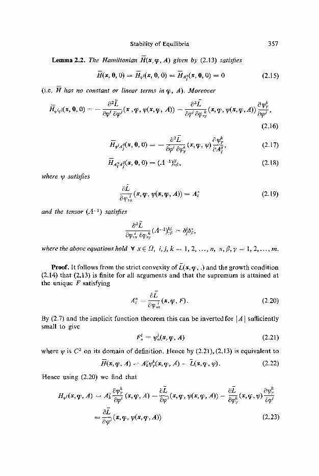
Lemma 2.2. The Hamiltonian H(x~ ~, A) given by (2.13) satisfies

H(x, O, O) = Hvi(x, O, O) = fflA~.(X, 0, 0) = 0 (2.15)

(i.e. H has no constant or linear terms in % A). Moreover

eq~ ~ ( x , ~, ~,(x, r X)) t~ ~ e~,~ e~J '

where ~p satisfies

H ~ . ( x , o, o) = (A-~) 5 , l J

~/(x,~,~ v,(x,w, A)) = A7

and the tensor (A -~) satisfies

r ~- l'~kj i

(2.16)

(2.17)

(2.18)

(2.19)

where the above equations hold V x E ~ , i,j, k = 1, 2, . . . , n, ~, fl, ~ = 1, 2 . . . . . m.

Proof. It follows from the strict convexity ofL(x, ~, .) and the growth condition (2.14) that (2.13) is finite for all arguments and that the supremum is attained at the unique F satisfying

el A~' = ~ (x, q~, F). (2.20)

By (2.7) and the implicit function theorem this can be inverted for I A[ sufficiently small to give

F~ = ~i(x, ~, A) (2.21)

where W is C 2 on its domain of definition. Hence by (2.21), (2.13) is equivalent to

H(x ,~ , A) ~ k _ = Akwv(x, % A) -L(x, ~, ~p). (2.22)

Hence using (2.20) we find that

eL = #q--~ (x, ~, ~p(x, q , A)) (2.23)


and k

- - . ~ 8 ~ . x HA~( x, 9% ~(x, ~v, A)) = ~f~(x, of, A) + Ak ~ ( , 9 ~, A)

= w'~(x, ~ , A ) .

By (2.20) and (2.21) it follows that y~ satisfies

6L A; = ~ (x, ~, V(~, ~e, A)).

8L 8~v k - - (x,% A)

(2.24)

(2.25)

Part (2.15) of the lemma new follows from (2.22)-(2.25) and Lemma 2.1. Similar calculations yield the remaining claims of the lemma.

w 2.2 Solving the Hamilton-Jacobi Differential Inequality

To recapitulate, we have succeeded in w 2.1 in replacing the problem of deter- ming P(x, u) satisfying conditions (i) and (ii) at the beginning of w 2 by that of determining a solution P(x, 9~) of (2.12). We now address the problem of constructing a solution of (2.12). We will first prove that (2.12) is always locally solvable in the following sense.

Proposition 2.3. Given Xo E [2 there exists 6 ~ 0 such that

o => ~ (,,,~) + H t x , ~ , - ~ ) v i~ t<~ ,

has a solution on B,~(Xo) for all e sufficiently small.

(2.26)

Proof. We expand the right-hand side of (2.26) in powers of q%" and observe that in order to prove that (2.26) hold for 19~t sufficiently small it is sufficient to prove that it is satisfied strictly by the lowest order terms in the expansion (since these dominate the expansion for [9~1 small).

Correspondingly, using (2.9), we write

fi~(x, r163 = �89 ~ ( x ) q/qfi + E~(x, 9~), (2.27)

where E ~ is of cubic or higher order in q~ and az~ = ~zj~. It now follows from Lemma 2.2 that the terms of lowest order in the expansion of the right-hand side of (2.26) are quadratic and given by

[ �89 I F (~i~(x)) ~'~J +/4~i,Ax, 0, 0) ~ J + 2ff~;4(~, 0, 0) ~d~jq~ k

(~Q x - -

(2.28)


Notice that only second derivatives of H with respect to the entries of A occur, since by (2.27) all derivatives of higher order contribute terms of cubic or higher order in the ~;.

It is thus sufficient to prove that the quadratic form in ~i given by (2.28) is uniformly negative definite on B~(xo) for some 6 > 0 for some choice of the coefficient functions (~r~} in (2.28).

To this end we choose

zr~i ~ zr(x) " i = 1, 2 . . . . . n (no summation) (2.29)

1 and all the other ~r~'s equal to zero. Now let ~r(x) = -- -~- (x -- x~) V x E B6(xo);

then all the terms in (2.28), except for those involving the first derivative of the coefficient functions ~r~, are bounded in B~(x). In fact (2.28) becomes

(v~ ') + ~,o~(x, o, o) q~'~ + 2ff~(~, o, o) ~ '~ , + H,,14(~, O, O) ~o'~,.

(2.30) Clearly by choosing ~ > 0 sufficiently small we can ensure that (2.30) is uniformly negative and hence that (2.26) holds for ]~ t sufficiently small for this choice of the Jr~'s. This completes the proof of the proposition.

The last proposition together with the arguments outlined at the beginning of w 1 yields the proof of the following theorem.

Theorem 2.4. Suppose that Uo E C2(~) is a solution of(2.2). Then given x o E f2 there exist e(Xo), ~(Xo) > 0 such that E(u) ~ E(uo) for all u -- u o E W~'P(B~(xo)), p > n with ]lU-- UoIIc< e(Xo).

We next establish conditions under which Uo is a strong local minimiser in the large (i.e. with no restriction on the size of the support of the admissible variations). This is the content of the next theorem. We will use (2.28) < (respectively (2.28) < ) to denote that the quadratic form given by (2.28) is negative definite

(respectively strictly negative definite) for all x E -Q.

Theorem 2.5. Suppose that uo E C: (~) is a solution of(2.2) and that there exists

a set o f coefficient functions {z~} in C ' ( ~ ) satisfying the differential inequality (2.28) < in ~ then Uo is a strong local minimiser of E: i.e.

E ( u ) ~ E ( u o ) Y u - - UoE W~'P(I2) with I l U - U o l l c < e , for some e > O .

This theorem will follow from the expansion arguments used in the proof of the

last proposition once we prove that (2.28) < has a solution throughout ~. This is the content of the next proposition.

Proposition 2.6. Suppose that the coefficient functions ( ~ j are in C1(f2) and satisfy the differential inequality (2.28) < in ~ . Then there exist (~r~) that satisfy (2.28) < in ~2.


Proof. Let

~i~(x) = 7r~. -t- n-i)(x) for i , j = 1, 2 . . . . . n, o~ = 1, 2 . . . . m, (2.31)

where the ~ ' s will be determined at a later stage. Then in order that {~i)} satisfy (2.28) < in f2 it is necessary and sufficient (since the {n~.} satisfy (2.28) -~ by assumption) that the {~i)} satisfy

{ ~ _ _

(~(x)) + 2H~,A~,(X, O, O) -~ ~ikX~t ~ + na~a~(x, O, O) -~

_ _ } o) :~,~:~j, + t4A.~4(x, o, o) ~ } ~'~ < o + ~a}(x, 0, ~-~ V x c ~ q .

(2.32)

other ~

Now let

~(x) = eexp -- [ + ( x ' -- c)], (xl) x 2

where k > 0 and c i s chosen so that x 1 - c > 0 V x = E ~.

xm

On substituting this expression for .~ into (2.33) and dividing by exp [-- k ( x ' - - c ) ] we obtain

--k~ic? i + 2eH#A](x, O, O) ~i~j + 2e~a]A~(X, 0, 0) =~0iq~ ~

+ e2ffA,A)(X, O, O)exp [~ek(x ' -- c)] ~i~'.

Choosing k = 1 and e sufficiently small, we see that this quadratic form is strictly negative definite. Hence (2.31) is a solution of (2.28) < throughout ~.

Remark 2.7. It is interesting to note the way in which the existence of a set of coefficient functions {'~t~} satisfying the conditions of the last Theorem (i.e. (2.28)-~) implies the positivity of the second variation of E(u) (given by (2.1)) at Uo. Notice first that by the definition of L, (2.5), all second and higher order derivatives of L with respect to u and Vu evaluated at Uo, VUo are equal to the corresponding derivatives of/7 when evaluated at 9~ = 0, Vg~ = 0. Hence

,. ~2LO . OZL ~ OL o . . 6 2 E ( u o ) ( r = 1 # , j

, f>a~s ~ a ~ s ~ . . a ~ Z o . = ~ ~Z~,~ ~'~'~ + 2 ~ , ' ~ , + ~ , ~ , - ( ~ , ~ J ) , ~ .

Choose ~]i(x)= •(x), i = 1, 2 . . . . , n (no summation) and all the equal to zero. On substituting this into the left-hand side of (2.32) we obtain

- - - - . . - - - - . . - - . .

(~),, cyqJ + 2H~,~!(x, O, O) 7t~'~' + 2HAJA~(X, O, O) nn~Cp'Cy § HAIA)(X , O, O) ~2Cp'Cp'.

(2.33)


(The addition of the divergence term contributes nothing to the second variation, by the divergence theorem, since ~ vanishes on ~ . ) Expanding the divergence term and rearranging then yields

>,. [ Lg,~ + (A-1)~

where (A-l) , defined as in Lemma 2.2, is the inverse of \c~<p,k #q0,~]" Notice that

our assumption of strict convexity of of L with respect to Vu implies that the first term in the integrand is nonnegative. It now follows from Lemma 2.2 that the condition that the coefficient functions {z~} satisfy (2.28) z is exactly equivalent to asking that the remaining term in the integrand, i.e.

e2Z~ (~Ta),=] ~kf~,

be a non-negative quadratic form in the 9~;'s, i.e. by subtracting the integral of an appropriate divergence from 82E(uo) (~ ,~ ) we have made the integrand nonnegative (and thus in particular 82E(uo) ( % ~) is also). The converse question as to whether positivity of the second variation implies the existence of a set of coefficient functions satisfying (2.28) < appears to be open and I hope to address this in a later paper.

Remark 2.8. In the one-dimensional case (m = n = 1) (2.28) < reduces to (12), the ordinary differential inequality given in the introduction. In this case it can be easily shown, by the continuation principle, that (2.28) -~ has a solution

on L) (which is an interval) if and only if (2.28)= is solvable on ~ . (2.28) = is known as Legendre's equation and in this case Remark 2.7 reduces to an observation of Jacobi--see BOLZA [4].) It is also interesting to note that, in this one- dimensional case, Legendre's equation transforms to the Jacobi conjugate point equation (i.e. the linearised Euler equation)under a nonlinear change of variables (see BOLZA [4]). Under this correspondence the existence of conjugate points can be shown to be equivalent to the nonexistence of a solution of Legendre's equation throughout the interval.

Remark2.9. For the one-dimensional case (m = n - - 1 ) TONELLI [22, H, p. 344] proves a result more powerful than Theorem 2.4 (see also BALL & MIZZL [20, p. 334]). A striking consequence of TONELLI'S theorem is that given any e > 0, there is a 8 > 0 with the property that E(u) ~ E(uo) V uE W~o'P((Xo -- 8, Xo -}- 8)) satisfying [I u -- Uo ]lc < e.


Example2.10. Let m = n = 1, L(x, u, u') = �89 [(u')2 -- u2], ~ = ( 0 , 2 ) , Uo ~ 0. Then (2.28)= (which is equivalent to (2.28) -~ in this case) becomes

:r'(x) + 1 ~ 7r2(x) ~ 0 x E [0, 2].

It is easily verified that this has solution :r(x) = tan (c -- x) and that no solution exists for 2 ~ zt.

w 3. The Polyeonvex Case

In this section we combine the ideas and results developed in the earlier sections to study the stability of equilibria, under zero body force, of an inhomogeneous elastic body which in its reference state occupies some bounded domain 3 2 Q R n, n = 1 ,2 ,3 . In the notation o f w this corresponds to the case

L(x, u, Vu) = W(x, Vu), (3.1)

where W: 32 x M"+• R + is the stored energy function of the material and

M n• = {FE mn• d e t F > 0}. (3.2)

Any deformation of the body u : 32-+ Rn satisfying the local invertibility condition

det (Vu(x)) > 0 for a.e. x C 32 (3.3)

has an associated energy E(u) given by

E(u) = f W(x, Vu(x)) dx. (3.4) s

The equilibrium equations, under zero body force, are the Euler-Lagrange equations for (3.4)

c~ (~W~ (x, Vu (x ) )~=O, xE.O, i = 1 , 2 , n. (3.5) t~x '~ \ c r ~ ] " '"

Definition 3.1. (i) I f n = 2 we say that the stored energy function W(x, F) is polyconvex if and only if there exists a convex function G : ~ x M 2 • cxz)

R+ such that

W(x, F) = G(x, F, det F) V F E M 2x2 Y x E f2. (3.6)

(ii) I f n = 3 we say that the stored energy function W(x, F) is polyconvex if

and only if there exists aconvex function G:.QxM3• oo)--~ R+ such that

W ( x , F ) = G ( x , F , adjF, detF) V F E M 3• V x E ~ (3.7)

where adj F and det F denote the adjugate matrix and determinant respectively.

We will assume throughout this section that W(x, Vu) is uniformly polyconvex in the sense that

W(x, F) = ~ ]F] 2 + W(x, F) V FE M "• for some ~ > 0, (3.8)


w h e r e / ~ x , .) is polyconvex and where G-will denote the corresponding convex function of the minors given by Definition 3.1. We will suppose for the purposes of

this section that G is C 2 on its domain of definition. Again throughout this section Uo will denote a smooth solution of (3.5).

The main result of this section is to demonstrate, in this polyconvex case, an analogue of Theorem 2.4 namely

Theorem 3.2. I f W(x, F) is polyconvex and Uo E C2(~) is a solution of (3.5), then, given Xo E f2, there exist e(Xo), 6(Xo) > 0 such that

E(uo + el) ~ E(uo) u q~ E W~'P(B~(xo)) with 1[~ l[c < e. (3.9)

We now outline the strategy of proof of this result: the idea is to use the observation from w 1 that in order to prove that uo minimises E(u) on A,,~ (given by (2.3)) it is necessary and sufficient that there exists afunctional ~ : A,,o ~ R such that

(i) E(u) => ~-(u) V u E ,'L,o, (3.10)

(ii) ~ ' (u) ~ o~-(Uo) u u C A~,o, (3.11)

(iii) ~-(Uo) ----- E(uo). (3.12)

In this section we do not assume that ~ is a null Lagrangian. Our choice of ~ is given by the integral of the right-hand side of (3.13), which we denote

L(x, Vu), and Lemma 3.3 shows that solutions of the Euler-Lagrange equations for E are automatically solutions of the Euler-Lagrange equations for ~ . It follows from this same lemma that our choice of ~ satisfies (i) and (iii). Hence it only remains to prove that ~ satisfies (ii). To this end we set u----Uo + r and demonstrate, in Proposition 3.4, that there is a null Lagrangian N(x,% Vg~ )

such that L(x, ~Uo + V~ )-- N(x, ~, V~) is strictly convex in V~ (in the case n = 3 this holds for I]~ ]lc sufficiently small). Since the addition of a null Lagran- gian does not change the variational structure of the integral functional Y ( u ) we can now apply our results from the convex case (i.e. Theorem 2.4) to conclude that (ii) and consequently Theorem 3.2 holds.

We will prove Theorem 3.2 in the case n ~-- 3, stating where necessary the corresponding result for the two-dimensional case.

It is a consequence of the assumption of polyconvexity and (3.8) that

w(x , Vu) > ,, IVul 2 + v Uo, adj VUo, det VUo)

( - + ~ (X, Vuo, adj Vuo, det VUo) u i

+ ~ (x, Vuo, adj Vuo, det Vuo) ((adj Vu)/~ -- (adj Vuo)~)

+ -~- (x, VUo, adj Vu o, det Vuo) (det Vu -- det Vuo) V u E A~,~.

(3.13)

364 J. S1VALOGANATHAN

We denote by L(x, Vu) the Lagrangian which is given by the right-hand side of the above inequality. The following lemma relates equilibria for f W(x, Vu)

to those of f L,(x, Vu). n f2

Lemma 3.3. I f uo is a solution of(3.5) then Uo is a solution of the Euler-Lagrange

equations for ~ ( u ) = f L(x, Vu) dx, f2

E(u) > ~ ( u ) V u ~ A~,~, (3.15)

and moreover

~(Uo) = f ~L(x, VUo) dx -= f W(x, Vuo) dx = E(uo). (3.16) O s

The proof of this lemma consists of a straightforward calculation and will be omitted.

Proposition 3.4. (i) I f n = 2 then there exists a null Lagrangian N(x, ~, V~) such that

L(x, VUo + Vq~) -- N ( x , % V~) (3.17)

is strictly convex in Vq).

(ii) I f n = 3 then there exists a null Lagrangian N(x, q~, V~) such that

[,(x, VUo + Vg~) -- N(x,r163 Vg~ ) (3.18)

is strictly convex in V~ for Hg~lic sufficiently small.

Proof. We prove the result in the case when n = 3. The case n ~ 2 follows by analogous arguments.

To prove the result it is clearly sufficient to prove that the Hessian of

/~(x, Vuo + Vt/~) -- N(x ,~ , Vq~) with respect to the gradient variable is strictly positive definite for some choice of null Lagrangian N. Hence it is sufficient to consider those terms in L(x, VUo + V ~ ) which are of quadratic or higher order in VW. These terms are

860 ~ o - - - ~i~v~ w ,~ =- ~!d ~ t e~,,~w,~,w,~'r ,7 + 3e e~Uo,~q) ,~q) ,~,).

(3.19) Now let

N(x, 9~,Vq~)=_�89176 .. . . ) , , ~ ' e ,J~ . . . . . s ,, '

/ ,~o ,,

This is easily verified to be a null Lagrangian. (It has the form of a divergence which vanishes on the boundary of ,(2.) On subtracting this null Lagrangian from (3.19)


we obtain

_,o, ko _ , ok ,

- w o �89 t - g D - ] ( 3 . 2 1 )

The only terms which are quadratic or higher order in Vq) are now the first and third terms in the above expression, i.e.

. . . . . . ( 3 . 2 2 )

It now follows from the fact that the first term is uniformly positive definite that the whole expression is a strictly positive definite quadratic form in Tq~ for []r sufficiently small.

We now apply Theorem 2.4 for the convex case to the integrand

L(x, rp, TqO = Z,(x, VUo -Jr- VW) --N(x, ep, VW) (3.23)

to conclude that ~ ~- 0 is a strong local minimiser in the small for f L(x, % V~) s

and hence that Uo is a strong local minimiser in the small for ~(u) = f L(x, Vu).

Finally, this together with Lemma 3.3 demonstrates that ~" satisfies (3.10)-(3.12) completing the proof of Theorem 3.2.

Remark 3.5. There is an obvious global version of this Theorem, with no restriction on the support of the admissible variations, which can be deduced by applying Theorem 2.5 to f L(x, ~, V~). However> one would not expect such a

result to be optimal in general. It is still open, in this polyconvex setting, as to whether the criterion of positivity of the second variation fails as a sufficient condition for a strong local minimiser. (See also Remark 2.7.) Work in BALL & MARSDE~ [3] shows that the criterion certainly fails for mixed displacement trac- tion problems.

Remark 3.6. Our proof of Theorem 3.2 shows indirectly that, for uniformly polyconvex integrands, the Hamilton-Jacobi inequality (1.19), as given in Pro- position 1.3, together with the boundary condition (1.20), is always locally solvable. An alternative approach to the construction we have used would be to work directly with the Hamilton-Jacobi inequality. The main problem that we would encounter is that the Hamiltonian H as defined by (1.21) is not in general smooth. However it is interesting to note that in these cases it is sufficient to solve

0 ~ ~ (x, u) 4- H(x, u, Vx,uP~, V,,Po) V x E ~ , V u E A, (3.24)


where

8P~ .. H(x, u, Vx,,P~,VuVo) = Sup ~ * o - , .

A=ad jTu (3.25) d=de tTu

8P~ } + ~ J~+ -- G(x, Vu, adj Vu, det Vu) ,

i.e., we treat the determinant, adjugate and gradient as independent variables.

The advantage of (3.24) is that f fwi l l be smooth if G is strictly convex and clearly a solution of this differential inequality will yield a solution of (1.19) since H ~ H . t

Our proof of (Theorem 3.2 can be interpreted in the spirit of the last remarks as having constructed a solution of (1.19) by solving a smooth generalised Hamil- ton-Jacobi inequality in which the Hamiltonian H is replaced by a smooth

Hamiltonian H which is an upper bound for H. We remark also that given any particular equilibrium the techniques we have

used in the proof of Theorem 3.2 may yield stronger results as demonstrated by the next example

Example 3.7. Let W(F) = tr (FrF)+ h (det F), where h is C a and strictly convex, then W is polyconvex. Let

[x' + v(x 2, x3)] U 0(X ) = / x 2 , , (3.26)

I X 3 ,

where ~ solves A ~ = 0 in ,(2. Then Uo represents a shear and is a solution of (3.5); since det V u o ( X ) ~ 1, (3.5) reduces to

duo = 0, (3.27)

and Uo clearly satisfies (3.27). In fact Uo is a global minimiser of E(u)for the displacement boundary value problem. This is a consequence of the following argument which is analogous to the proof of Theorem 3.2: by the convexity of h

E(u) ~ f tr (VurVu) + h (det Vuo) + h' (det Vuo)(det Vu -- det Vuo)dx . a

Since Uo is an isoehoric deformation, it follows that the last term in the integral is a null Lagrangian with integral zero. Now by the convexity of tr (VurVu) and (3.27) it follows that

f tr (Vu r Vu) + h (det Vuo) dx ~ f tr (Vug" Vuo) + h (det Vuo) dx = E(uo). g2

* Related notions are used by PONTE CASTANEDA [I 5] in the study of overall properties of nonlinear composites; see also TALBOT • WILLIS [16] for the use of comparison functionals.


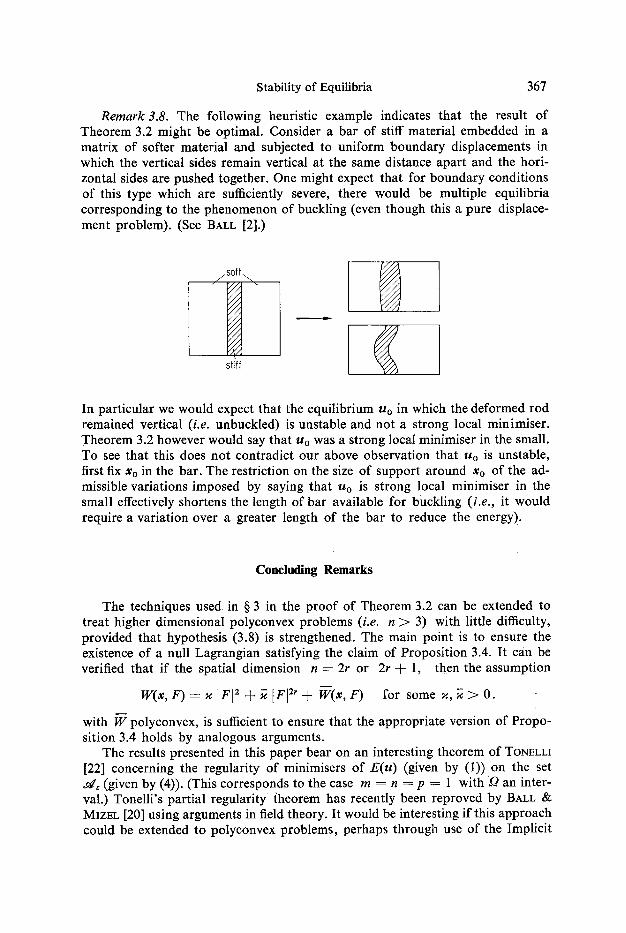
Remark 3.8. The following heuristic example indicates that the result of Theorem 3.2 might be optimal. Consider a bar of stiff material embedded in a matrix of softer material and subjected to uniform boundary displacements in which the vertical sides remain vertical at the same distance apart and the hori- zontal sides are pushed together. One might expect that for boundary conditions of this type which are sufficiently severe, there would be multiple equilibria corresponding to the phenomenon of buckling (even though this a pure displacement problem). (See BALL [2].)

/solf...~

stiff

In particular we would expect that the equilibrium Uo in which the deformed rod remained vertical (i.e. unbuckled) is unstable and not a strong local minimiser. Theorem 3.2 however would say that Uo was a strong local minimiser in the small. To see that this does not contradict our above observation that Uo is unstable, first fix Xo in the bar. The restriction on the size of support around Xo of the admissible variations imposed by saying that Uo is strong local minimiser in the small effectively shortens the length of bar available for buckling (i.e., it would require a variation over a greater length of the bar to reduce the energy).

Concluding Remarks

The techniques used in w 3 in the proof of Theorem 3.2 can be extended to treat higher dimensional polyconvex problems (i.e. n ~ 3) with little difficulty, provided that hypothesis (3.8) is strengthened. The main point is to ensure the existence of a null Lagrangian satisfying the claim of Proposition 3.4. It can be verified that if the spatial dimension n = 2r or 2r -4- 1, then the assumption

W(x, F) ---- ~ IF[ 2 -1- ~ IF] 2r 4- W(x, F) for some z, ~ > 0.

with W polyconvex, is sufficient to ensure that the appropriate version of Propo- sition 3.4 holds by analogous arguments.

The results presented in this paper bear on an interesting theorem of TONELLI [22] concerning the regularity of minimisers of E(u) (given by (1)) on the set d e (given by (4)). (This corresponds to the case m = n = p = 1 with ~ an interval.) Tonelli 's partial regularity theorem has recently been reproved by BALL & MIZEL [20] using arguments in field theory. It would be interesting if this approach could be extended to polyconvex problems, perhaps through use of the Implicit


Function theorems of VALENT [23] and the results of w 3. (Regularity of minimisers under the assumption of strict quasiconvexity is studied in EVANS [8].)

I remark finally that it would be interesting to relax the smoothness assump- tions made in this paper. (For example, allowing non-smooth potentials P ~ should make it easier to satisfy (1.20).) In this context the work of LIONS [18] should be relevant.

Acknowledgements. I thank GARETH PARRY for useful discussions and JOHN BALL for constructive suggestions concerning the manuscript. My thanks also to JOHN TOLAND for comments on the one-dimensional problem which in part motivated the approach I have taken in this paper.

References

1. J. M. BALL, Convexity conditions and existence theorems in nonlinear elasticity, Arch. Rational Mech. Anal. 63 (1977), 337-403.

2. J. M. BALL, Constitutive inequalities and existence theorems in nonlinear elastostatics, "Nonlinear Analysis and Mechanics": Heriot-Watt Symposium Vol. 1 (R. J. KNOPS Ed.), Pitman (London), 1977, 187-241.

3. J. M. BALL d~ J. E. MARSDEN, Quasiconvexity at the boundary, positivity o f the second variation and elastic stability, Arch. Rational Mech. Anal. 86 (1984), 251-277.

4. O. BOLZA, "Lectures on the Calculus o f Variations", Dover Publications Inc., 1961. 5. G. A. BLISS, "Lectures on the Calculus o f Variations", University of Chicago Press,

1946. 6. L. CESARI, "Optimisation--theory and applications", Springer-Verlag, 1983. 7. B. DACOROGNA, "Weak continuity and weak lower semi-continuity o f nonlinear

functionals", Springer-Verlag, Lecture notes in Mathematics, vol. 992, 1982. 8. L. C. EVANS, Quasiconvexity and partial regularity in the Calculus o f Variations,

Arch. Rational Mech. Anal. 95 (1986), 227-252. 9. P. J. OLVER, Conservation laws and null divergences, Math. Proc. Camb. Phil. Sac.

94 (1983), 529-540. 10. P. J. OLVER & J. SIVALOGANATHAN, The structure o f null Lagrangians, Nonlinearity 1

(1988), 389-398. 11. H. RUND, "The Hamilton-Jacobi theory in the Calculus o f Variations", Van Nostrand

(London), 1966. 12. J. SIVALOGANATHAN, A field theory approach to stability o f radial equilibria in nonlinear

elasticity, Math. Proc. Camb. Phil. Sac. 99 (1986), 586-604. 13. J. SIVALOGANATHAN, Implications o f rank one convexity, Analyse Non Lin6aire 5

no. 2 (1988), 99-118. 14. H. WEYL, Geodesic Fields, Ann. Math. 36 (1935), 607-629. 15. P. PONTE CASTENEDA, On the overall properties o f nonlinearly elastic composites,

(Preprint) Dept. of Mech. Eng., The Johns Hopkins University, Baltimore, U.S.A. (1988).

16. D. R. S. TALBOT & J. R. WILLIS, Variational principles for inhomogeneous nonlinear media, I .M.A.J. Appl. Math. 35 (1985), 39-54.

17. R. B. VINTER & R. M. LEWIS, A verification theorem which provides a necessary and sufficient condition for optimality, I.E.E.E. Trans. on Automatic control AC-25 no. 1 (1980), 84-89.

18. P. L. LIONS, "Generalised solutions o f Hamilton-Jacobi equations", Research notes in Mathematics, no. 69, Pitman, Boston, 1982.


19. D. G. B. EDELEN, The null set of the Euler-Lagrange operator, Arch. Rational Mech. Anal. U (1984), 117-121.

20. J. M. BALL & V. J. MIZEL, One-dimensional variational problems whose minimisers do not satisfy the Euler-Lagrange equation, Arch. Rational Mech. Anal. 90 (1985), 325-388.

21. J. M. BALL & J. C. CURRIE & P. J. OLVER, Null Lagrangians, weak continuity and variational problems of arbitrary order, J. Funct. Anal. 41 (1981), 135-174.

22. L. TONELLI, "Fondamenti di Calcolo delle Variazioni", Zanichelli 2 vols. 1, 11, 1921- 1923 (in L. Tonelli, Opere Scelte voL 13, Edizioni Cremonesi, Roma, 1961).

23. T. VALENT, "Boundary valueproblems of finite elasticity", Springer Tracts in Natural Philosophy voL 31, Springer-Verlag, 1988.

School of Mathematical Sciences University of Bath Claverton Down Bath BA 2 7AY

U.K.

(Received December 5, 1988)

Date post:	01-Jul-2018
Category:	Documents
Upload:	vomien
View:	215 times
Download:	0 times

The generalised Hamilton-Jacobi inequality and the ...masjs/Research Papers/HJinequality.pdf ·...

Documents