DISCUSSION PAPER SERIES Forschungsinstitut zur Zukunft der Arbeit Institute for the Study of Labor The Geographic Accessibility of Child Care Subsidies and Evidence on the Impact of Subsidy Receipt on Childhood Obesity IZA DP No. 6025 October 2011 Chris M. Herbst Erdal Tekin
Transcript
DI
SC
US
SI
ON
P
AP
ER
S
ER
IE
S
Forschungsinstitut zur Zukunft der ArbeitInstitute for the Study of Labor
The Geographic Accessibility of Child Care Subsidies and Evidence on the Impact of Subsidy Receipt on Childhood Obesity
IZA DP No. 6025
October 2011
Chris M. HerbstErdal Tekin
The Geographic Accessibility of Child Care Subsidies and Evidence on the
Any opinions expressed here are those of the author(s) and not those of IZA. Research published in this series may include views on policy, but the institute itself takes no institutional policy positions. The Institute for the Study of Labor (IZA) in Bonn is a local and virtual international research center and a place of communication between science, politics and business. IZA is an independent nonprofit organization supported by Deutsche Post Foundation. The center is associated with the University of Bonn and offers a stimulating research environment through its international network, workshops and conferences, data service, project support, research visits and doctoral program. IZA engages in (i) original and internationally competitive research in all fields of labor economics, (ii) development of policy concepts, and (iii) dissemination of research results and concepts to the interested public. IZA Discussion Papers often represent preliminary work and are circulated to encourage discussion. Citation of such a paper should account for its provisional character. A revised version may be available directly from the author.
The Geographic Accessibility of Child Care Subsidies and Evidence on the Impact of Subsidy Receipt on Childhood Obesity*
This paper examines the impact of the spatial accessibility of public human services agencies on the likelihood of receiving a child care subsidy among disadvantaged mothers with young children. In particular, we collect data on the location of virtually every human services agency in the U.S. and use this information to calculate the approximate distance that families must travel from home in order to reach the nearest office that administers the subsidy application process. Using data from the Kindergarten cohort of the Early Childhood Longitudinal Study (ECLS-K), our results indicate that an increase in the distance to a public human services agency reduces the likelihood that a family receives a child care subsidy. Specifically, we estimate an elasticity of subsidy receipt with respect to distance of -0.13. The final section of the paper provides an empirical application in which we use variation in families’ travel distance to identify the causal effect of child care subsidies on children’s weight outcomes. Our instrumental variables estimates suggest that subsidized child care leads to sizeable increases in the prevalence of overweight and obesity among low-income children. JEL Classification: I12, I18, J13, R53 Keywords: child care, subsidy, obesity Corresponding author: Erdal Tekin Department of Economics Andrew Young School of Policy Studies Georgia State University P.O. Box 3992 Atlanta, GA 30302-3992 USA E-mail: [email protected]
* Chris Herbst gratefully acknowledges funding support from the W.E. Upjohn Institute for Employment Research. We thank Matthew Neidell for providing us with the data on car ownership rates. Alexander Brumlik provided excellent research assistance.
Created alongside the passage of welfare reform in 1996, the Child Care and Development
Fund (CCDF) is the primary funding stream devoted to child care assistance in the U.S.2 Indeed,
child care subsidies have been playing an increasingly important role in government efforts to reduce
welfare caseloads and increase employment among economically disadvantaged families. Yet
despite these goals, the take-up rate for child care subsidies—defined as the fraction of eligible
families receiving assistance—remains low. For example, recent studies estimate that approximately
15 to 30 percent of the eligible population is being served (Herbst, 2008; U.S. DHHS, 1999). The
low take-up rate is largely attributed to the CCDF’s funding structure as a close-ended block grant,
but subsidy participation rates continue to be low in states that devote relatively more resources to
child care assistance (U.S. DHHS, 2000) and among families that are explicitly targeted by state
administrators (Schumacher & Greenberg, 1999). This suggests that a combination of demand- and
supply-side factors play an important role in influencing subsidy utilization.
In this paper, we examine one such factor that has been largely ignored by previous research:
the spatial accessibility of public human services agencies. Proximity to a local agency can impact
subsidy receipt during multiple stages of a family’s interaction with the subsidy system. In
particular, many parents are required to make one or more personal visits to an agency to conduct the
initial in-take and eligibility screening (Adams, Synder, & Sandfort, 2002). The number of office
visits largely depends on state-specific rules governing the stringency of income and employment
documentation and the extent to which families require assistance locating suitable child care
providers. In addition, parents in many jurisdictions are required to report in-person all changes to
employment and income. This can be particularly challenging for low-income parents, who have
2 In addition to the annual CCDF allocation, states may transfer up to 30 percent of their Temporary Assistance to Needy Families (TANF) grant
to fund child care assistance through the CCDF. These transfer funds are subject to most of the eligibility rules in the CCDF. Another policy that
provides child care assistance is the Child and Dependent Care Tax Credit (CDCTC). Created in 1976, the CDCTC initially provided a non-refundable credit of $4,800 (2+ children) for child care expenses incurred. Tax legislation in 2001 expanded the CDCTC by allowing families to
claim additional child care expenses and increasing the credit rate for families below $43,000. However, expenditures on the program remain
modest (at $2.8 billion as of FY 2006), and it still operates as a non-refundable tax credit, making benefits largely inaccessible to low-income families (Burnam, Maag, & Rohaly, 2005).
3
less access to automobile transportation and are more likely to experience frequent job turnover,
seasonal or irregular work hours, and highly volatile earnings. Finally, policies regarding eligibility
recertification in some states require parents to make multiple trips to the local human services
agency. In particular, the time-limited nature of child care subsidies—usually lasting three to 12
months—implies that parents need to restart the eligibility process every few months or risk benefit
termination. Again, the ease with which families are able to complete the recertification process
depends on the number and types of documents required and whether parents are able to schedule
appointments with caseworkers at convenient times.
At least two other factors interact with states’ subsidy policies that make spatial accessibility
a particularly important consideration for low-income families. First, it is plausible that families are
more likely to apply for child care subsidies if they have sufficient information about the program’s
operation and requirements. Access to such knowledge is likely to be greater when the relevant
agencies are located close to home. Indeed, previous studies find that information and awareness are
important determinants of participation in other programs, including food stamps (Daponte et al.,
1999) and Medicaid (Aizer, 2007). Second, human services agencies located close to home may
increase families’ trust in these institutions. If potential subsidy recipients view local agencies as
invested in the success of surrounding neighborhoods, such individuals could be more likely to apply
for assistance.
Low utilization rates have long been a source of concern for many means-tested programs,
but the take-up of child care subsidies is substantially lower than those of other social welfare
programs (Witte & Queralt, 2002). For example, take-up rates range from 43 percent for the
Qualified Medicare Beneficiary program to 99 percent for Medicare Part A (Witte & Queralt, 2002).
Take-up rates for other well-known programs are also relatively high: 40 percent for TANF (Crouse,
Douglas, & Hauan, 2007), 60 percent for Food Stamps (Pavetti & Rosenbaum, 2010), and about 87
percent for the school lunch program (Currie, 2003). As the recent economic downturn continues to
4
leave millions of people unemployed, a record number of people are turning to the social safety net
to ease their hardship. Furthermore, Congress in the next few years will reauthorize the Personal
Responsibility and Work Opportunity Reconciliation Act (PRWORA), the 1996 welfare reform
legislation that created the current child care subsidy system. As a result, it is increasingly important
to understand how means-tested programs can be redesigned to help low-income individuals access
relevant benefits.
Aside from its policy significance, an analysis of the geographic proximity of public human
services agencies provides researchers with a unique opportunity to study the influence of child care
subsidy policy on outcomes related to children and parents. To arrive at credible estimates of the
impact of subsidy receipt, researchers must deal with a number of well-known selection problems
(Berger & Black, 1992; Gelbach, 2002). In particular, given that child care benefits are not randomly
distributed to eligible families, those who utilize a subsidy may differ systematically from those who
do not in ways that are not captured by researchers. If these unobserved determinants of subsidy
receipt are correlated with the outcome of interest, estimates of the impact of subsidy policy will be
biased. Unfortunately, finding exogenous sources of variation in subsidy receipt is difficult, and this
has slowed progress in this important policy domain.3
Therefore, our measure of the spatial accessibility of public human services is offered as a
potentially useful way to leverage quasi-experimental variation in subsidy utilization. In particular,
it might be possible to identify the impact of subsidy receipt on a range of policy-relevant outcomes
by exploiting geographic variation in families’ travel distance to the nearest agency. Using the
distance measure as an instrumental variable for subsidy receipt is equivalent to comparing the
outcomes of children and mothers who face different probabilities of subsidy receipt because they
reside different distances to human services agencies. As with all instruments, our proposed distance
3 These identification problems are frequently cited by child care scholars as one of the primary explanations for the diversity of estimates generated in the maternal employment literature (Anderson & Levine, 2004; Blau & Tekin, 2007; Blau, 2001; Tekin, 2007).
5
measure must satisfy two conditions to serve as a valid exclusion restriction, namely it must be
highly correlated with child care subsidy receipt and it must be uncorrelated with the outcomes
except through its impact on subsidy receipt. We provide evidence throughout the paper that both
conditions are likely to be met.
To demonstrate the usefulness of the distance measure as an instrumental variable, we
conduct an analysis of the impact of child care subsidies on childhood obesity. The prevalence of
childhood obesity has risen substantially over the last three decades and is now one of the most
pressing public health concerns facing U.S. children. In recent work, Herbst and Tekin (2011a) use
data from the Kindergarten cohort of the Early Childhood Longitudinal Study (ECLS-K) to
investigate the relationship between subsidy receipt in the year before kindergarten and children’s
weight outcomes in the fall and spring of kindergarten. The authors find that subsidized care is
associated with increases in body mass index (BMI) and a greater likelihood of being overweight and
obese. Although the authors control for a large number of observable characteristics that are likely to
be correlated with preferences for child care subsidies and children’s health, lingering concerns over
the endogeneity of subsidy utilization do not permit a causal interpretation of the results. In this
paper, therefore, we revisit the analysis of children’s weight outcomes using the distance measure to
produce credible estimates of the effect of child care subsidy receipt on childhood obesity.
The remainder of this paper is organized as follows. Section II provides a summary of the
supply- and demand-side factors that explain parental decisions regarding subsidy utilization. Section
III discusses the conceptual framework and empirical model for the relationship between parents’
travel distance and subsidy use. In section IV, we introduce the survey data as well as describe the
steps taken to create the distance measure. Section V presents various estimates of the impact of
proximity to these agencies on the likelihood of receiving subsidized child care. In section VI, we
use the distance measure to instrument for subsidy receipt in an analysis of children’s weight
outcomes. Finally, section VII offers conclusions and a discussion of policy implications.
6
II. Background
This study contributes to the literature on the analysis of demand- and supply-side
determinants of child care subsidy receipt. Studies of demand-side explanations usually find that
young, unmarried women with greater numbers of young children are more likely to receive child
care assistance. Furthermore, subsidy recipients are simultaneously more likely to be employed and
receive other means-tested benefits. Interestingly, the likelihood of subsidy receipt is greater among
families with relatively high levels of education, possibly because of the skills necessary to navigate
the complex application process (Durfee & Meyers, 2006; Blau & Tekin, 2007; Herbst, 2008; Tekin
2005; 2007).
As for supply-side factors, low program awareness is frequently cited as being prohibitive,
even though most states now conduct public awareness campaigns. For example, one study finds
that 44 percent of eligible non-applicants are unaware of their eligibility (Schlay et al., 2004). High
transaction costs also appear to be important factors. Recent interviews with parents and
caseworkers in 12 states reveal administrative barriers to subsidy participation (Adams, Synder, &
Sandfort, 2002). In particular, the authors find that parents must communicate with a large number
of administrative agencies to access and retain a subsidy. The frequency of eligibility recertification
and the requirement that caseworkers be notified of all changes to income and employment are also
cited by families as being resource- and time-consuming.
A sizeable body of work finds that measures of geographic accessibility are strongly
associated with work and welfare outcomes as well as participation in a variety of social services and
means-tested programs. For example, Allard and Danziger (2003) find that job accessibility and
proximity to employment opportunities increase the likelihood that low-income families find work
and leave welfare. Allard, Tolman, and Rosen (2003) show that greater spatial proximity to social
service providers increases the probability that welfare recipients receive these services. Neidell and
Waldfogel (2009) analyze the impact of local Head Start availability on immigrant children’s
7
participation. The authors find that having a Head Start center in a child’s census tract significantly
increases the likelihood of enrollment. It has also been shown that the distance to medical care
facilities is positively correlated with health care utilization (e.g., Nemet and Bailey, 2000) and
treatment intensity for acute myocardial infarction (McClellan et al., 1994). Geographic variation in
the proximity to college campuses during childhood appears to be highly correlated with later college
attendance (Card, 1995). Finally, Bertrand et al. (2000) show that social networks, as defined by
proximity to services among those in the same language group, are an important determinant of
welfare participation.
There is considerable indirect evidence that decisions regarding child care subsidy receipt are
likely to be sensitive to the geographic accessibility of agencies administering these programs. For
example, one study finds that mothers’ daily trip from home to the child care provider adds 28
percent more time to the total commute (Michelson, 1985). It is therefore not surprising that low-
income working mothers, in particular, stress the importance of locating child care services close to
home or work (Henly & Lyons, 2000). Another study finds that nearly 70 percent of low-income
parents rate ―conveniently located services‖ as very important to their child decisions, compared to
50 percent among high-income parents (U.S Department of Education, 1995). These preferences
appear to translate in practice: a study of child care subsidy recipients in Cuyahoga County, Ohio
finds that such families travel approximately two miles to center-based providers and 1.5 miles to
family daycare homes (Bania et al., 2000).
III. Conceptual Framework and Empirical Model
Economic models of program participation provide a structured approach to thinking about
the impact of spatial accessibility on child care subsidy receipt (e.g., Moffitt, 1983). In particular,
parents are predicted to apply for and receive assistance when the benefits of doing so exceed the
costs. In this framework, the distance to a local agency represents real costs in terms of travel time,
transportation expenditures, and foregone earnings. Therefore, parents in communities with less
8
spatial accessibility to a public human services agency face higher costs and thus greater constraints
on subsidy participation. Many of these costs are compounded by the limitations of public
transportation in high-poverty neighborhoods and low car ownership rates among low-income
families (Allard, 2009; Berube & Raphael, 2005; Ong, 2002). With single mothers’ commute times
averaging 10 hours per week (Edin & Lein, 1997), greater distances to human services agencies
make it increasingly difficult to fulfill the program obligations discussed above. It is therefore
expected that less spatial accessibility to a local agency reduces the likelihood of subsidy utilization.
Formally, let a mother’s utility in the absence of a child care subsidy be expressed as U(Y; X,
L), where Y is private income, X represents demographic preference shifters, and L is a set of
geographic characteristics that shape families’ decision-making. If a mother receives a subsidy, her
utility is expressed as U(Y + M; X, L) – D, where M captures the potential benefits of receiving child
care assistance and D represents the disutility associated with program participation. The benefits of
subsidy receipt include the increase in net-wages that results from decreased child care expenditures.
The disutility of subsidy participation is related to the time, psychic, and transportation costs
associated with trips to public human services agencies.4 It is further assumed that D is an increasing
function of the distance between mothers’ residential location and the nearest agency.
A mother will therefore decide to receive a child care subsidy if U(Y + M; X, L) – U(Y; X,
L) > D, that is, if the utility gain from receiving subsidized care exceeds the disutility. Based on this
simple model, the decision to utilize child care subsidies can be expressed by the following equation:
(1) Si = Xiβ1 + β2di+ Liβ3 + εi
where Si is an indicator of subsidy receipt for the ith potentially eligible mother, Li is a set of local
characteristics such as the availability of other services that are potential substitutes for child care
4 Another potential benefit of receiving a child care subsidy could be improved child well-being if it is used to purchase a high-quality child care
arrangement. This would be formalized by including child quality as another argument in the mother’s utility function. However, this is not necessary for the purposes of this paper. Another potential cost of receiving a child care subsidy could be stigma. However, we do not explicitly
focus on stigma since it is largely unobserved and difficult to separate from transaction costs and information (Moffitt, 1983; Neidell &
Waldfogel, 2009). In addition, the literature suggests that other costs associated with the take-up of social programs are more important than stigma (Currie, 2004).
9
subsidies (e.g., church services, Head Start, etc.); X is a set of child and family characteristics that
could influence the decision to take-up a child care subsidy, and εi is an idiosyncratic error term. The
di is the measure of spatial accessibility, defined as the approximate distance (in miles) between
families’ residential location and the nearest public human services agency. We create two
parameterizations of the travel distance. First, we incorporate the natural logarithm of the distance to
allow for a linear relationship. We then test a non-parametric version of the distance measure by
including dummy variables for the quartiles of the distance distribution. In results available upon
request, we also experiment with quadratic and higher-order polynomials in the distance measure.
However, in each case only the linear term is statistically significant. The coefficient of interest is β2,
which captures the impact of distance on the probability of receiving a subsidy. Our main testable
hypothesis is that the probability of subsidy receipt decreases with the distance to the nearest social
welfare agency (i.e., β2=δS/δd < 0). We estimate versions of (1) using a linear probability model
(LPM).5
A potential concern with this estimation strategy is that our distance measure could be
determined in part by the joint location preferences of families and human services agencies. For
example, administrative offices might locate in low-income neighborhoods in order to be accessible
to potentially eligible clients. In addition, given the low rates of car ownership among disadvantaged
families, such individuals may prefer to reside near critical support services or employment and
public transportation centers. If these unobserved neighborhood characteristics determine the
relative location of families and agencies, the coefficient on the distance measure will be biased.6
5 The least squares estimates of coefficients in LPMs are consistent estimates of average probability derivatives, but the standard errors are biased
as a result of heteroskedasticity. We report standard errors that are robust to any form of heteroskedasticity. Since our distance measure is based, in part, on families’ residential census tract, the standard errors are adjusted for clustering at the census tract-level. Our results are robust to
clustering at the county-level. We also estimate (1) using probit and logit regression. Marginal effects from these models are very similar to
those from the LPM. 6 It is important to note that in some states the same human services agency provides access to multiple benefits (eg., cash assistance and child
care subsidies). If some areas are more likely to operate in this manner than other areas (eg., rural versus urban areas), it could be the case that
endogenous location choices for families and agencies are stronger (or at least operate differently) across these areas. However, we have not been able to uncover any evidence that the choice of service provision is correlated with states’ urbanicity.
10
Recent empirical work finds little support for the notion that individuals Tiebout sort across
space in order to access government-provided goods and services (Rhode & Strumpf, 2003).
Furthermore, while endogenous location choices are plausible for entitlement programs or services
with open-ended funding streams, we argue that it is highly unlikely that low-income parents move
to a given neighborhood to be close to an agency administering child care subsidies. These benefits
are heavily rationed by local agencies (because of the close-ended block grant funding structure),
suggesting that the supply of subsidies is outstripped by demand. As a result, it is common for
parents to experience frozen intake and long waiting lists (Herbst, 2008). Children receiving
subsidized care do so for only short periods before restarting the eligibility process, and all interim
income and employment changes must be reported to caseworkers. Therefore, it seems fairly risky to
choose a residential location based on the location of child care administrators. As pointed out by
Allard (2009), the location choices of social service agencies are constrained in a number of ways.
These constraints help to explain why one-fifth of the social service agencies in his three-city study
had been operating in the same location for six to 10 years, and over half were in the same location
for more than 10 years. As a result, social service agencies are unlikely to adjust rapidly to changes
in the geographic distribution of low-income families.
Nevertheless, we take a number of steps in the empirical analysis to mitigate the influence of
endogenous location choices. Our preferred specification adds county fixed effects, which capture
unobserved local determinants of the demand for child care subsidies that may bias the coefficient on
di. In addition to removing the influence of county- and state-level demographic and economic
characteristics, county fixed effects control for the availability of substitute forms of early care and
education (Li), which may affect the demand for a child care subsidy. The fixed effects also account
for unobserved CCDF policies that are correlated with the spatial location and availability of human
services agencies. For example, some jurisdictions allow families to apply for assistance via mail,
11
telephone, or the web.7 It is also plausible that some counties conduct outreach campaigns to raise
awareness of subsidy programs as well as provide parents with support services to access local
agencies.
In robustness checks, we add detailed controls for the neighborhood environment (i.e., census
tract) in which families and agencies are located. In addition, separate models experiment with a
vector of school fixed effects. Together, the census tract controls and school fixed effects could be
more effective than the county fixed effects at controlling for factors in the neighborhood
environment that lead families and agencies to systematically sort in space. As a final robustness
check, we take advantage of two questions in the ECLS-K that permit more explicit controls for
endogenous location choices. The first question asks parents whether (and how times) the family
moved since the birth of the focal child. The second question inquires about whether the home
location was chosen because of local school characteristics. Nearly two-thirds of families in our
sample moved at least once since childbirth, and one-quarter of parents chose the current home
location because of local school characteristics. Therefore, these are potentially important
preference-shifters that could be correlated with the travel distance and subsidy receipt.8 In each
robustness check, the coefficient on travel distance is not noticeably different from that of our
preferred specification using county fixed effects.
IV. Data
Our data come from the Early Childhood Longitudinal Study–Kindergarten cohort (ECLS-
K). The ECLS-K is a nationally representative sample of 21,260 children attending kindergarten in
7 As of 1998, 14 states in our ECLS-K sample allowed families to request subsidy applications mail, telephone, or email (Alaska, Arizona,
Arkansas, Kansas, Louisiana, Maine, Michigan, Missouri, Oregon, Pennsylvania, South Dakota, Tennessee, Texas, and Washington). Another five states (Maine, Michigan, Oregon, Texas, and Washington) allowed families to complete the subsidy application via mail or telephone. 8 The fraction of movers is consistent across the distance distribution. However, we find some evidence that the home location variable is
correlated with travel distance. Fully 23 percent of parents at the first quartile of the distance distribution responded that they chose the home location because of school characteristics, increasing to 30 percent among parents at the fourth quartile of the distribution. These differences,
which are statistically significant, largely disappear when basic controls for the neighborhood environment are introduced. The rate of subsidy
receipt is higher among movers (8.5 percent compared to four percent) and lower among families choosing the home location because school of characteristics (5.8 percent compared to 7.5 percent).
12
the fall of 1998.9 Children in the ECLS-K are followed through the eighth grade, with detailed parent
interviews and child assessments conducted in the fall and spring of kindergarten (1998 and 1999)
and the spring of first (2000), third (2002), fifth (2004), and eighth (2007) grade. The analyses in
this study are based on the fall of kindergarten wave of data collection, in which parents are asked
about child care experiences, including subsidy participation, in the year prior to kindergarten entry.
Our analysis sample includes families potentially eligible for child care subsidies. To be
eligible for CCDF funds, families must have at least one child ages 0 to 13; parents are required to
participate in a state-defined acceptable work activity; and total income must fall below 85 percent of
the state median income. In practice, however, the extraordinary amount of state variation in
eligibility rules creates difficulties for precisely simulating eligibility (Giannarelli et al., 2001; Witte
& Queralt, 2003). Therefore, we define the analysis sample to include families in the bottom three
quintiles of the full sample socioeconomic status (SES) distribution.10 Our final analysis sample
includes 9,231 children.11
An implication of limiting the sample to potentially eligible families is that the subsidy
participation rate is likely to be an underestimate of the take-up rate. Indeed, approximately seven
percent of families in our sample receive a child care subsidy, whereas studies that carefully simulate
eligibility find participation rates between 15 percent and 30 percent (e.g., Herbst, 2008). It is
important to note that we experiment with several alternative sample selection criteria, including
explicit attempts to define a low-skilled sample (e.g, mothers with less than a B.A degree), an
income- and employment-based eligible sample (e.g., families below 85 percent of a state’s median
income and working mothers), and those whose demographic characteristics are highly correlated
with subsidy receipt (e.g., unmarried mothers). In no case do these alternatives materially change the
9 For more information on the ECLS-K, see Herbst and Tekin (2010a, 2011). 10 Created by ECLS-K administrators, the SES index is based on parental education and occupation and total family income. 11 To create the analysis sample, we dropped additional observations if there was missing information on the census tract identification number
(2,256 observations), missing information on the entire parent interview (740 observations), missing information on the child care subsidy receipt question (35 observations), and mothers with nonsensical ages (6 observations).
13
results discussed below.12
The outcome variable in our analysis is a binary indicator for whether a child received
subsidized, non-parental child care in the year prior to kindergarten. Parents are asked a series of
questions about child care use during the previous year, including the number of arrangements, the
amount of time that each arrangement was used, whether there was a cost associated with each
arrangement, and if so, the amount paid for care. Regarding subsidy receipt, parents were asked the
following: ―Did any of the following people or organizations help to pay for this … provider to care
for {CHILD} the year before {he/she} started kindergarten?‖ Four possible choices were then
presented to parents, and we coded those answering ―a social service agency or welfare office‖ as
receiving a child care subsidy.13
The primary right-hand-side variable is a measure of the spatial accessibility of local public
human services agencies, defined as the distance (in miles) that families must travel from home in
order to reach the nearest office that administers the subsidy application process. Appendix A
provides a detailed description of the steps taken to generate the distance measure, so we include
only a brief discussion here.14 The process began by creating a database containing the precise
location (building number, street name, city, state, and zip code) of every public human services
agency in the U.S. In doing so, we were careful to ensure that a given agency is involved in
eligibility and benefit determination for CCDF child care subsidies. Our database contains location
information on over 3,600 human services agencies.15 The next step in the process involved
12 The estimated effect of families’ travel distance on subsidy utilization in column (4) of Table 1 (the full model) is -0.009**. When the sample definition is changed to low-skilled mothers, the coefficient on travel distance is -0.007**. Similarly, when the sample includes eligible families,
as defined by the CCDF rules (i.e., family income is less than 85 percent of a state’s median income or the mother is employed), the coefficient
on travel distance is -0.006**. Thus, our results are robust to changes in the sample definition. 13 As described in the conceptual framework, this variable allows us to model the parental decision to apply for and receive a child care subsidy.
We do not model decisions regarding child care arrangements, although subsidy receipt has been shown to be associated with a shift to formal
child care settings (Tekin, 2005; 2007). For example, in our analysis sample, 25 percent of unsubsidized children are in parent care, while no subsidized children receive this care. A little over seven percent of unsubsidized children enroll in center-based services, compared to 38 percent
among their subsidized counterparts. Therefore, it is conceivable that our results on travel distance and subsidy receipt may indirectly apply to the
relationship between travel distance and the choice of child care provider. For example, given the negative relationship between travel distance and subsidy receipt documented in this paper and the positive correlation between subsidy receipt and formal child care enrollment found by
previous studies (Tekin, 2005; 2007), it is possible that increases in travel distance reduce probability of attending formal child care. 14 The forthcoming discussion and Appendix A are drawn from Herbst and Tekin (2010b; 2011b). 15 The public human services agency database will be made available to researchers upon request.
14
geocoding the location of administrative offices by assigning a latitude and longitude coordinate to
each. In an overwhelming number of cases (95 percent), we were able to assign a geocode based on
either the agency’s exact location or its census block. Only five percent of offices were geocoded at
the city- or zip code-level.16 In the final step, we calculated the Euclidean (or as-the-crow-flies)
distance between the location of human services agencies and the centroid (or geographic center) of
the census tract in which ECLS-K families reside. We generate the distance measure based on
families’ census tract because residential addresses are not available in the ECLS-K. In addition,
given that states’ child care subsidy programs are administered primarily at the county-level, we use
families’ county of residence as the geographic boundary for calculating the distances.
A potential concern with using the census tract centroid to create the travel distance is that it
introduces a form of aggregation error (Hewko et al., 2002). This type of measurement error plagues
spatial accessibility indicators that are aggregated to a geographic unit of analysis (in this case, the
census tract) that varies substantially in size. Given that the land area associated with residential
census tracts differs dramatically across ECLS-K children, a distance measure based on the
geographic center of census tracts introduces non-random measurement error into the distance
calculations.17 In particular, the amount of error has been shown to increase with the size of the
geographic unit (Apparicio et al., 2003; Apparicio et al., 2008; Pone et al., 2006). Large census
tracts are more common in suburban and rural areas, suggesting that our distance measure could be
less precise for families in these neighborhoods.18 We attempt to deal with aggregation error in
several ways. In the robustness analyses, we begin by controlling for census tract population density,
which depends in part on its land area (defined as square miles). We then estimate models that
control explicitly for land area. Finally, we estimate two-stage least squares (2SLS) regressions that
16 Our results are robust to the exclusion of these agencies from the calculation of the travel distance. 17 The median child in our analysis sample resides in a census tract that is 1.5 square miles. There is, however, considerable variation in the census tract land area. For example, the range is 0.02 square miles to 6,521 square miles, and the standard deviation is approximately 139 square
miles. 18 The median child in an urban area lives in a census tract that is 1.1 square miles. The comparable figure for children in rural areas is 35.4 square miles.
15
alternately use the average county- and zip code-level travel distance as an instrument for families’
travel distance. Our main results are robust to these specification checks.
Following the literature on the determinants of child care subsidy receipt, we include in the
model a detailed vector of controls for child and family characteristics. The child variables include
status, and first-time kindergartner. The set of family characteristics includes maternal age and
educational attainment, family structure, number of other children in the household, whether English
is the spoken language at home, and the log of household income. We also incorporate binary
indicators to control for missing observations on each of our control variables.
V. Results
Results from equation (1) are shown in Table 1. The top panel presents results from models
that use the natural logarithm of the distance to the closest agency.19 By employing the natural
logarithm, we mitigate the influence of outliers in determining regression coefficients. In addition,
we allow for non-linearities in the relationship between the distance measure and subsidy receipt by
including binary indicators for the second, third, and fourth quartiles of the distance distribution
(binary indicator for the first quartile is the omitted category). These results are presented in the
bottom panel. In column (1), we display the basic results from models that only include the distance
variable. In columns (2) and (3), we add child characteristics and family characteristics, respectively.
In column (4), we incorporate county fixed effects.
As shown in the top panel of Table 1, the coefficient on the distance measure is negative and
statistically significant in all models, indicating that an increase in the distance to the nearest public
human services agency reduces the likelihood that a family receives a child care subsidy. The
coefficient in column (4) implies that a one-percent increase in the mileage to the nearest agency
19 Note that there are multiple agencies to choose from in some counties. In those cases, the distance measure represents the distance to the closest agency.
16
decreases the probability of subsidy utilization by 0.9 percentage points. This estimate yields an
elasticity of child care subsidy receipt with respect to distance of -0.13.
The results in the bottom panel of Table 1 suggest that the probability of subsidy receipt
decreases monotonically as families reside greater distances from the closest public human services
agency. Families located in the third and fourth quartiles of the distance distribution are 2.2 and 2.6
percentage points less likely to receive a subsidy than those in the first quartile, respectively. Those
in the second quartile are about one percentage point less likely to receive a subsidy than those in the
first quartile, although the coefficient is not precisely estimated.
Table 2 presents results from a number of robustness checks and sub-group analyses. In
terms of robustness checks, we add several controls to further account for the possibility of
endogenous location choices among parents and human services agencies. First, we incorporate a
rich set of controls for the census tract in which ECLS-K families and agencies reside.20 Second, we
remove the county fixed effects and add school fixed effects, which serves as another proxy for
neighborhood characteristics that may capture unobserved location preferences. If anything, these
additional location controls have the effect of making the distance coefficient more negative,
suggesting that unobserved location preferences cause the OLS estimates to understate the true effect
of families’ travel distance.21
Finally, we attempt to more explicitly control for parental location preferences by adding
binary indicators for whether the family moved since the focal child’s birth and whether the parents
chose the home location because of school characteristics. To the extent that school characteristics
are correlated with the availability and attributes of local social services, controlling for this variable
20 The family census tract controls are population density, percent females ages 16+ employed, percent ages 0-17, percent ages 65+, percent
employed in local government, percent employed in state government, percent ages 25+ with less than a high school degree, and percent foreign
born. The agency census tract controls are log of median household income, log of population density, percent non-Hispanic white, percent foreign born, percent ages 65 and over, percent female, percent of households receiving welfare, and percent of employed females ages 16 and
over. The model including the agency controls omits the county fixed effects but includes school fixed effects. We do this because, due to data
exigencies, the agency characteristics are aggregated up to the county-level. We also estimate a model that includes the family and social service agency characteristics simultaneously (along with school fixed effects). Results are robust to this specification. 21 This makes sense: if agencies indeed choose to reside near potential clients, the distance should be positively correlated with factors associated
with socioeconomic status. This implies that a regression model that fails to take these factors into account would result in estimates that are biased toward zero.
17
may further mitigate the potential bias associated with endogenous location choices. As shown in
Table 2, our results are robust to the inclusion of these controls.
In results available upon request, we implement a falsification test to gain more confidence
that we account for unobserved heterogeneity. Specifically, we estimate our most comprehensive
model replacing the outcome of subsidy receipt with a binary indicator for whether a parent has
obtained a bachelor’s degree or more.22 The idea is that the distance to the nearest public human
services agency should not predict an outcome that is unlikely to be influenced by child care subsidy
receipt. As expected, we find that the distance to the nearest agency is uncorrelated with the
educational attainment of low-skilled mothers. In particular, the impact of the natural logarithm of
the distance measure on the likelihood that a mother has at least a college education is statistically
and economically insignificant, with a coefficient of 0.0014 and a p-value of 0.52.
The next set of robustness checks attempt to account for measurement error in the travel
distance that arises from using the geographic center of census tracts of different sizes to construct
the distance measure. Our first strategy is to control explicitly for the land area of each census tract.
As previously stated, the vector of census tract controls described above includes population density,
defined as a ratio of each neighborhood’s total population to its land area. Inclusion of this (and the
other) neighborhood controls do not alter the main results. We also enter land area and land area
squared directly into the model, and find that these controls do not influence the coefficient on the
distance measure. Interestingly, neither of the land area variables is statistically significant. Our
second strategy instruments for families’ travel distance using average distance measures aggregated
to both the county- and zip code-levels. The first-stage F-statistic on the aggregated county and zip
code distance is, respectively, 78.8 and 233.6, indicating a strong correlation between families’ travel
distance and the aggregated distance instruments. As shown in Table 2, the second-stage results
22 However, we implement this exercise excluding from the analysis the sub-set of parents who are currently attending school. This exclusion is
necessary because subsidy receipt can induce parents to engage in work or work-related activities, such as attending school. Therefore, distance measure may indirectly affect the current schooling by affecting the decision to receive a subsidy.
18
continue to show a negative and statistically significant relationship between families’ travel distance
and subsidy utilization. In addition, the instrumental variables estimates are fairly close in magnitude
to the OLS results, suggesting that the county fixed effects and neighborhood controls mitigate the
influence of systematic measurement error in the distance measure.
In the final set of robustness checks, we test alternative distance measures. Recall that the
results presented so far are based on the distance to the closest public human services agency.
Approximately one-third of families in our dataset live in jurisdictions that contain multiple agencies
administering CCDF subsidies. To account for the presence of multiple agencies, we create a
distance variable based on the sum of the inverse distances, which is advantageous because it gives
more weight to agencies that are closer to families’ residential location. The coefficient suggests that
a one-percent increase in the mileage to the local administrative office reduces the likelihood of
subsidy receipt by 1.1 percentage points
The remaining results in Table 2 explore the possibility of heterogenous effects of families’
travel distance. In particular, when we estimate the models separately for families residing in urban
and non-urban areas, the impact of distance is substantially larger among those in non-urban areas.23
This finding is plausible given that access to public transportation and major roadways is likely to be
more restricted in non-urban areas. Furthermore, human services agencies are distributed over larger
land areas in rural counties, resulting in longer travel distances for families residing in these
jurisdictions.24
Next, we estimate models separately for states that do and do not allow families to request or
complete subsidy applications through the mail, telephone, or web. It is important to reiterate that
although some parents may not be required to visit an office for the initial application and eligibility
screening, there are numerous factors subsequent to this that may necessitate in-person visits
23 We define urban as residence in a census-defined city (of any size) or another census-designated urban area. 24 Indeed, the average distance to the closest agency in urban areas is 6.52 miles, compared to 12.37 miles in non-urban areas.
19
(Adams, Synder, & Sandfort, 2002). Therefore, it is plausible that distance continues to be costly for
families that are allowed to submit subsidy applications through alternative means. Our results
appear to corroborate this intuition: increases in the distance measure are associated with a
statistically significant reduction in subsidy receipt irrespective of whether families must make
personal visits to the local public human services agency.
We also examine the extent to which access to reliable transportation differentially influences
the role of distance in determining subsidy participation. It is possible, for example, that the impact
of distance is substantially greater among families facing high transportation costs because of low car
ownership rates. In other words, if the distance to an agency influences subsidy participation by
altering transportation costs, we might expect lower subsidy participation rates among families with
low car ownership rates. To test this, we merge the ECLS-K data with household car ownership rates
calculated at the census-tract-level, and use this information to divide neighborhoods into ―high‖ and
―low‖ car ownership neighborhoods.25 We then estimate the full model separately for families in
each of these neighborhood-types. Consistent with our expectation, the distance measure has a
greater impact on subsidy participation among families with higher transportation costs (residing in
―low‖ car ownership neighborhoods) than those with lower transportation costs (residing in ―high‖
car ownership neighborhoods).
Finally, we estimate models separately by families’ cash assistance status (receipt of
AFDC/TANF or food stamps). Interestingly, the results indicate that distance serves as an obstacle
to subsidy receipt only for those families not receiving other forms of cash assistance. To the extent
that families receiving welfare and food stamps have already committed to traveling to agencies,
25 These data are drawn from the 2000 Decennial Census. Neighborhoods coded as having ―high‖ car ownership rates are those in which the
fraction of households owning zero cars is at or below the 25th percentile of the distribution or those in which the fraction of households owning two or more cars is at or above 75th percentile of the distribution. All other neighborhoods are coded as ―low‖ car ownership neighborhoods.
20
distance should be less influential in the decision to apply for and receive other forms of assistance,
including child care subsidies.26,27
To put our results into perspective, a number of simulations are conducted in which we
calculate the predicted probability of subsidy utilization if families face travel distances at the 20 th,
10th, and 5th percentiles of the full sample distance distribution. The mileage at these percentiles
corresponds to travel distances of 1.9, 1.2, and 0.9 miles, respectively. These predicted probabilities
are also compared to a ―baseline‖ prediction that uses the sample mean of the distance measure (7.7
miles) to calculate the utilization rate. The simulations are conducted for all families, and separately
for families living in urban and non-urban areas. As shown in the top panel of Table 3, reducing
families’ travel distance from the mean to the 5th percentile of the distance distribution increases the
predicted subsidy utilization rate from seven percent to 8.5 percent. This represents a 21 percent
increase in the predicted utilization rate. Not surprisingly, reductions in the travel distance lead to
substantially greater increases in subsidy receipt among non-urban families than urban families, as
shown the second and third panels. For example, the anticipated effect of reducing the travel
distance to the 5th percentile among urban families is to increase the participation rate from seven
percent to eight percent, an increase of 14 percent. The identical reduction in the travel distance for
non-urban families increases the predicted subsidy participation rate from seven percent to 12
percent, an increase of nearly 76 percent. Therefore, one of the key policy implications of our results
is that the subsidy take-up rate could be increased by relocating agencies closer to low-income
neighborhoods, particularly in rural areas, where travel distances tend to be substantially longer and
families are more sensitive to the costs of establishing and maintaining subsidy eligibility.
26 It is plausible that several of the variables used to create the sub-groups actually belong in the main subsidy utilization model. For example, the indicators for urban residence, AFDC/TANF/food stamp receipt, and census tract car ownership rates could be important determinants of subsidy
utilization. We therefore test the robustness of the main results with these variables added, and find that their inclusion does not substantially
change the estimated effect of families’ travel distance on subsidy receipt. The coefficient (and standard error) on the log of distance to social service agencies is -0.007* (0.004) with these variables included. 27 In results available upon request, we estimate the model separately for white non-Hispanic families and all other racial and ethnic groups. Both
sets of families respond similarly to an increase in the distance to human social services agencies. However, the estimates are less precisely estimated due to smaller sample sizes.
21
To provide additional context for potential policy implications, we estimate the full model
separately for families residing in counties with a single public human services agency and those
with access to multiple agencies. Our results suggest that families’ travel distance is strongly
associated with subsidy utilization among parents with access to just a single agency, but much less
strongly associated with subsidy receipt among parents who may chose between multiple agencies.
In particular, a one percent increase in travel distance is associated with a 1.3 percentage point
decrease in the subsidy participation rate among parents living in counties with a single agency. The
corresponding figure for parents living in counties with multiple agencies is 0.05 percentage points.
Unlike the policy simulations above, which decreased the average travel distance for select families
(while holding constant the number of accessible agencies), this analysis provides initial evidence
that increasing the number of administrative offices may similarly increase the subsidy utilization
rate.
VI. Empirical Application: Child Care Subsides and Children’s Weight Outcomes
Introduction and Discussion of the Conceptual Framework
A potential benefit of our agency database is that it presents a unique opportunity to study the
impact of child care subsidies on outcomes related to children and parents. One such possibility is an
analysis of the relationship between subsidy receipt and low-income children’s weight outcomes. As
mentioned earlier, childhood obesity is one of the most pressing public health problems in the United
States. Over the past three decades, the prevalence of childhood obesity increased from five percent
to 10.4 percent among two- to five-year-olds and from 6.5 percent to 19.6 percent among six- to
eleven-year-olds (Ogden, et al., 2008; Ogden et al., 2010). Severe weight problems during childhood
are associated with a variety of short- and long-term consequences, ranging from childhood
depression and poorer academic achievement to lower wages and continued health problems
percent of eligible subsidy recipients (Herbst, 2008).29 Our final analysis sample includes 3,742
children in the fall of kindergarten and 3,577 in the spring of kindergarten.
We are concerned with three measures of children’s weight throughout kindergarten: BMI 28 See Herbst and Tekin (2010a) for a detailed discussion of the sample creation. To be included in the sample, children must reside with a
biological mother only, a biological mother and a partner ―father,‖ an unmarried adoptive mother who may or may not be living with a partner
―father,‖ or an unrelated, unmarried guardian who may or may not be living with a partner ―father.‖ Exclusions from the sample are made if the child is missing information on all outcome variables (1,766) or the entire fall of kindergarten parent interview (740), the questions regarding
child care subsidy receipt (35), and census tract identifiers (2,256). We exclude an additional 12,607 children who do not meet our requirements
for residence with an unmarried mother. 29 Note that this sample definition differs from the one used in the analysis of the impact of travel distance on subsidy utilization (i.e., bottom
three quintiles of the SES distribution). To elaborate on the discussion in the text, we change the sample to single mothers for two reasons. First,
we want to be consistent with Herbst and Tekin (2011). Second, SES depends in part on family income, which could introduce a form of sample selection bias. In particular, if family income determines which families use child care subsidies and it affects children’s weight outcomes, we
are concerned that conditioning the sample on income could bias the estimated effect of subsidy receipt. Nevertheless, we test the robustness of
our main weight results by examining two alternative sample definitions: low-education mothers and families below 85 percent of the state median income. Results from these models are similar to those presented here.
25
and binary indicators of overweight and obesity status. The measure of BMI is calculated as weight
in kilograms divided by height in meters squared (kg/m2). For children ages two to 19, BMI values
are plotted on growth charts from the Centers for Disease Control (CDC) to determine the
corresponding BMI-for-age percentile. Children at or above the 85th percentile of the gender- and
age-specific BMI distribution are coded as overweight, and children at or above the 95th percentile of
the BMI distribution are coded as obese. Approximately 28 percent of children in our sample are
overweight (30 percent for subsidized children versus 28 percent for unsubsidized children) in the
fall of kindergarten, and 13 percent are obese (12 percent for subsidized children versus 13 percent
for unsubsidized children).
We begin the analysis by estimating a reduced form OLS model to capture the relationship
between child care subsidy receipt and children’s weight outcomes in the fall and spring of
kindergarten. Formally, this model is specified as follows:
(2) Wi = α0+ α1si + Xiα2 + Niα3 + νs + εi,
where Wi is one of three weight outcomes for the ith child, si is a binary indicator of child care
subsidy receipt, and X is a vector of observable family background characteristics that may be
correlated with children’s weight outcomes.30 Also included in the model is a set of census tracts
characteristics, N, to proxy the neighborhood environment in which families reside and a set of state
fixed effects, νs, to capture state-level policy, economic, and demographic factors that are associated
with subsidy utilization and child well-being. The coefficient of interest in (2) is α1, which provides
an estimate of the average difference in BMI and overweight/obesity prevalence between subsidy
recipients and non-recipients, conditional on the covariates in the model.
Given that si takes a value of one for all subsidy recipients (and zero for all non-recipients),
30 The child characteristics include gender, age, race, premature birth, low birth weight, disabled, and first time kindergartner. Family
characteristics are mother’s age, mother’s educational attainment, mother’s fair/poor health status, family type, number of children in the family, English as the primary spoken language in the family, and log of total family income. Finally, census tract/school controls include log of median
household income, log of population density, percent non-Hispanic white, percent foreign born, percent ages 65 and over, percent female, percent
of children ages 0-2 and 3-5 living in female-headed households, percent of children in the school eligible for free/reduced price lunch, an indicator for whether a majority of children in the school are minorities, and an indicator for whether the school receives Title I funding.
26
an assumption imposed by the empirical framework is that of homogenous policy treatments and
treatment effects across space (e.g., states or counties), child care providers, and dosages of subsidy
receipt. This is clearly a strong assumption. States and localities vary substantially in the
administration of their subsidy systems, including, most crucially, the operation of eligibility and
benefit reimbursement rules. Furthermore, subsidy policy by design allows children to enroll in a
variety of child care arrangements, some of which are included in the formal market while others
operate outside states’ regulatory regimes. Finally, child care subsidy spells are known to occur in
relatively short spurts, and it is common for children to experience multiple spells within a brief time
period (Ha, 2009). These considerations suggest that it is prudent to interpret α1 as averages of
heterogeneous effects of subsidy receipt across children exposed to varying amounts of the policy
treatment and who operate in different policy and child care environments.31
As is well-known in the child care literature, the selection of families into subsidized child
care raises concerns that subsidy participants and non-participants differ systematically in ways that
researchers are not able to capture. If these selection mechanisms are correlated with measures of
child well-being, the coefficient on subsidy receipt will be biased. For example, it is plausible that
highly motivated mothers or those with strong work preferences are more likely to request child care
assistance. Failure to control for maternal motivation and other relevant characteristics would lead to
an upward bias in the impact of subsidy receipt if these characteristics positively influence child
outcomes. It is also possible that subsidy administrators systematically ration child care benefits
according to specific household characteristics. For example, there are reasons to believe that
caseworkers target both the lowest- and highest-skilled mothers in order to meet work participation
31 Of course, we would like to utilize data on the hours per day each child receives subsidized care as well as the length of time each child has received a subsidy. However, such data are not available in the ECLS-K. We could, in principle, allow the effect of subsidies to vary across the
child care arrangements (which are collected by the ECLS-K), but including these arrangement in the model would introduce another endogeneity
problem. As discussed in the text, we somewhat relax the assumption of homogeneous treatment effects by conducting the analysis on sub-groups of children defined by maternal education level and SES.
27
targets. These possibilities suggest that subsidy receipt is correlated with unobserved program
characteristics, which, if left unmeasured, would bias the coefficient on subsidy receipt.
To produce credible estimates of the impact of subsidy policy on children’s weight outcomes,
we offer our measure of families’ approximate travel distance to the closest public human services
agency as a potential instrumental variable. Such an instrument must meet two conditions. It should
be correlated with the endogenous right-hand-side variable—in this case, subsidy receipt—and it
should be uncorrelated with the outcome of interest—in this case, measures of children’s weight—
expect through its relationship with subsidy receipt. The previous sections provide intuitive and
empirical evidence that families’ travel distance is in fact correlated with subsidy utilization in a
sample of potentially eligible families. Results in Herbst and Tekin (2010b) show that this
relationship is even stronger for children of unmarried mothers. Regarding the second criterion,
Herbst and Tekin (2010b) provide detailed arguments for why families’ travel distance can be validly
excluded from models of child outcomes. To conserve space, we provide only a brief summary of
those arguments here.
There are several threats to the validity of the distance instrument. First, it was mentioned
earlier that the travel distance could be determined by the joint location preferences of families and
agencies. If these unobserved family and agency preferences influence travel distance in ways that
influence children’s weight outcomes, the coefficient on subsidy receipt will be biased. As discussed
in this paper and elsewhere (Herbst & Tekin, 2010b), the CCDF’s structure as a close-ended block
grant coupled with its low take-up rate make it highly unlikely that parents would chose to live near
an agency that determines subsidy eligibility and benefit levels. As pointed out in Allard (2009),
local governments are constrained in a variety of ways that make it difficult for agencies to adjust to
short-run changes in the residential patterns of low-income families. Second, the distance measure
may proxy the extent of isolation from the social safety net, including access to such means-tested
programs as SNAP and WIC, both of which may influence children’s weight outcomes. Failing to
28
account for these factors would invalidate our instrumental variables strategy.32 Finally, it is possible
that families’ travel distance is a proxy for unobserved family and neighborhood attributes that
influence child well-being. For example, mothers who face a short travel distance to the nearest
agency may do so because they live in heavily populated (urban) and low-income neighborhoods.
Conversely, it is possible that those with longer distances are located in rural areas with racially
homogenous populations and constrained access to employment opportunities.33 To the extent that
the neighborhood environment directly affects child well-being or is correlated with resident family
characteristics, we might be worried that variation in the travel distance is systematically related to
variation in children’s weight outcomes. If these environmental factors are correlated with the travel
distance and are not properly accounted for in the weight model, the distance measure would not
constitute a valid instrument.
Table 4 explores the extent to which child and maternal characteristics are random with
respect to the travel distance before and after accounting for the neighborhood environment (Herbst
& Tekin, 2010b).34 In particular, column (1) shows the F-statistic (and p-value) from a test of the
null hypothesis of the equality of child and maternal characteristics across the quartiles of the
distance distribution prior to conditioning on the neighborhood environment. It is clear from the
reported F-statistics that many of these family characteristics are correlated with the travel distance.
For example, we find that families residing close to a public human services agency are less likely to
be white, more likely to have low levels of education, and have lower incomes than those residing far
away from an agency. Such differences justify our concern that the distance measure is a potential
proxy for family and neighborhood attributes that may be correlated with children’s weight
32 We thank an anonymous referee for bringing this possibility to our attention. 33 For the purposes of a study on childhood obesity, a critical neighborhood characteristic is the extent to which individuals have limited access to healthy food options. Such ―food deserts‖ are particularly likely to be found in low-income areas, where the single mothers in this study are
disproportionately located. See Sparks et al. (2011) for a detailed review of research on the spatial distribution of food deserts across high- and
low-income areas. 34 These controls are: log of median household income, log of population density, percent non-Hispanic white, percent foreign born, percent ages
65 and over, percent female, percent of children ages 0-2 and 3-5 living in female-headed households (all at the census tract-level), percent of
children in the school eligible for free/reduced price lunch, an indicator for whether a majority of children in the school are minorities, and an indicator for whether the school receives Title I funding (all at the school-level).
29
outcomes. However, the story changes dramatically in columns (2) through (5), which present the
child and maternal characteristics after conditioning on the (demeaned) neighborhood controls.
These family characteristics are now randomized over the distance distribution, and even critical
background characteristics like socio-economic status, maternal education, and family income are
uncorrelated with travel distance after accounting for the family’s neighborhood context. Indeed, the
adjusted F-statistic (and p-value) in column (6) reveals that, with the exception of children’s race,
there are no statistically significant differences in background characteristics across the distribution
of the travel distance. Such results indicate that neighborhood environment is responsible for the
observed family-level differences across the distance distribution, and as long as these controls are
included in the model, the distance measure can serve as a potentially valid instrument.
Nevertheless, we take a number of steps to mitigate the potential threats to the validity of the
distance instrument. First, we control extensively for the neighborhood environment in which ECLS-
K families live. Specifically, we include 11 census tract- and school-level variables in the weight
model. These variables capture several dimensions of neighborhoods’ wealth and resources,
urbanicity, racial and ethnic composition, and family structure that are either potentially correlated
with families’ location preferences or directly related to child well-being. Second, we incorporate a
comparable set of five controls for the neighborhood environment in which agencies are located.
These controls account for the unobserved determinants of agency location decisions that may also
be correlated with the distance families must travel to apply for public benefits. Third, we include a
vector of state fixed effects to account for state-level policy, economic, and demographic
unobservables that may influence child well-being or are related to the spatial configuration of public
human services agencies. Finally, in robustness checks, we attempt to further account endogenous
location choices by adding controls for whether the family chose its residential location based on the
characteristics of local schools and whether a family moved since the birth of the focal child.
As mentioned above, the jurisdictions that govern child care subsidies differ in a variety of
30
ways. For example, some of these jurisdictions are urban while others are rural. There is also
substantial variation in the networks of local roads and highways and the systems of public
transportation across these jurisdictions. The results in Table 2 confirm that access to subsidies
varies by urbanicity and local access to transportation. Such insights suggest that constraining the
relationship between travel distance and subsidy receipt to be the same for mothers across all
jurisdictions might mask many of these jurisdiction-level differences that are likely to interact with
the distance to influence subsidy utilization. To address this issue, we allow the subsidy impact to
differ by county of residence, which typically constitutes a jurisdiction. Therefore, our identification
strategy exploits this county-level variation in travel distance by interacting families’ travel distance
with a set of county-of-residence indicators. 35 With a p-value substantially less than 0.01, the set of
distance-county interactions is highly statistically significant in the first-stage equation.
Results
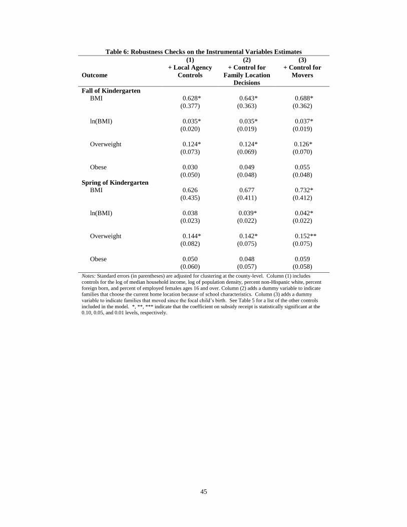
Table 5 presents the main results from our analysis of the impact of child care subsidies on
children’s weight outcomes. The top panel presents estimates using the fall of kindergarten weight
outcomes, and the bottom panel explores these outcomes in the spring of kindergarten. We begin by
estimating a simple OLS regression of each weight outcome on the binary indicator of child care
subsidy receipt [column (3)], followed by an OLS model that includes the full set of child and family
variables, neighborhood and school controls, and state fixed effects [column (4)]. Finally, we present
the instrumental variables estimates derived from two-stage least squares (2SLS). To conserve
space, we show only the coefficient on subsidy receipt, along with its standard error (in parentheses),
which is adjusted for county-level clustering.
Looking first at the fall of kindergarten results, we find that the OLS coefficient on subsidy 35 To investigate this issue, Herbst and Tekin (2010a) produce county- and state-specific correlations between the distance measure and subsidy
receipt. As expected, both sets of correlations are negative on average, but the amount of variation is substantially greater among counties, as
evidenced by a comparison of the standard deviations: 0.305 for the county-specific correlations and 0.172 for the state-specific correlations. Additional evidence of between-county variation in the distance-subsidy relationship is provided by comparing correlations across urban and
rural counties. Not surprisingly, the average correlation in rural counties is nearly three times larger than that in urban counties, but the spread of
correlations around the mean is also greater (SD rural: 0.397 versus SD urban: 0.277).
31
receipt is positive in the BMI and overweight models and negative in the obesity models, although in
no instance is estimate statistically significant. Furthermore, in most cases the magnitude of the
coefficient implies a subsidy effect that is close to zero. Our instrumental variables estimates, on the
other hand, imply sizeable and statistically significant impacts of subsidized child care. For example,
our results indicate that children receiving a child care subsidy in the year before kindergarten enter
school with a BMI that is 3.5 percent higher than that for non-recipients. In addition, subsidized
children are 11.9 percentage points more likely to be overweight and 4.8 percentage points more
likely to be obese. The same pattern emerges for the spring of kindergarten weight outcomes, with
subsidized children obtaining BMIs that 3.8 percent higher and rates of overweight and obesity that
are, respectively, 14.5 percentage points and five percentage points higher than their unsubsidized
counterparts.
We subject these results to a number of specification checks to ensure robustness. The
plausibility of the 2SLS estimates hinges on the validity of the key identifying assumption:
conditional on the observable family and neighborhood controls and state fixed effects, the distance
instruments can be excluded from the weight models. This assumption would be violated if there are
unobserved family and agency location choices that jointly determine the distance instrument and are
correlated with children’s weight. The IV results presented in Table 5 already condition on the
neighborhood environment in which ECLS-K families live. We take this analysis a step further by
also controlling for the characteristics of neighborhoods in which agencies are located. In doing so,
we are able to purge the effects of confounding location preferences on both sides of the child care
subsidy market. Results from this exercise, which are shown in column (1) of Table 6, show that the
subsidy estimates are robust to the inclusion of agencies’ neighborhood characteristics.
To further guard against the confounding effects of endogenous residential location choices,
we utilize an item in the ECLS-K that asks whether a given family chose its current home location
based on the attributes of local schools. Assuming that the demand for certain school characteristics
32
is highly correlated with parental preferences regarding other public services, including this variable
in the model should further purge the 2SLS estimates of bias resulting from unobserved family
location choices. As shown in column (2) of Table 6, our subsidy estimates are robust to the
inclusion of this preference variable. Next, we add a control for whether the family moved since the
focal child’s birth. Generally speaking, this variable should account for the opportunity to choose a
home location based on the accessibility social services among families that have higher propensities
to move. As shown in column (3), our subsidy estimates are once again robust to the inclusion of
this variable.36
Next, we conduct a falsification test to provide one more piece of evidence in support of the
validity of the distance instrument. If our identifying assumption is valid, then a variable predicting
child care subsidy receipt should not affect children in families that are highly unlikely to be eligible
for assistance. Since all families in the ECLS-K have children, we focus the falsification test on two-
parent families in the top two quintiles of the SES distribution. We first estimate the first-stage
subsidy receipt equation on the sample of single mothers in order to calculate a predicted probability
of subsidy receipt for the subset of two-parent families in the top SES quintiles. We then include this
variable in the child production function. The falsification test provides no evidence against the
validity of our identification strategy: in no case do we find that predicted subsidy receipt influences
the well-being of children in high SES two-parent families.
In final set of analyses, we explore the possibility of heterogeneous subsidy impacts across
sub-groups of children and mothers. Generally speaking, the estimates are substantially larger
among boys and among children living with a low-skilled mother. We do not find much
heterogeneity across children of different races and ethnicities. Subsidized boys experience an
increase in BMI of 6.8 percent and a rise in obesity rates of 9.1 percentage points, whereas the
36 We also estimate the model limiting the sample to those who did not move since the birth of the focal child. The coefficients on subsidy receipt are similar in sign and magnitude to the main results, although they are less precisely estimated due to a dramatic drop in the sample size.
33
relevant estimates for girls are 0.6 percent and 0.8 percentage points, respectively. The differences
across maternal education are striking. Among children with low-skilled mothers (defined as those
with a high school degree or less), subsidy receipt is expected to increase BMI by 4.6 percent and the
likelihood of obesity by 11.5 percentage points. Conversely, our estimates imply that subsidy receipt
lowers BMI and decreases the probability of obesity among children with high-skilled mothers
(defined as those with some college or above). Indeed, these subsidized children have BMIs and
obesity rates that are, respectively, 2.7 percent and 10.8 percentage points lower than their
unsubsidized counterparts.
These divergent estimates by maternal education suggest that the employment effects of
subsidy receipt may be more economically rewarding for high-skilled parents. The greater returns to
work for such parents could be used to make further health investments in children that ultimately
reduce the likelihood of obesity. It is also possible that increases in education lead to stable and
flexible jobs, which in turn might allow mothers to allocate more time to the production of health for
their children. Furthermore, high-skilled mothers could be more likely to find jobs with health
insurance, which may also reduce the likelihood of obesity among their children. In any case, these
differing results indicate that the subsidy effect is not homogenous over the distribution of maternal
education. Given that most states currently ration child care assistance, such heterogeneity suggests
that giving priority to high-skilled mothers has the twin advantages of not only assisting states in
meeting the stringent employment targets set forth by welfare reform, but it may also reduce the
prevalence of obesity within this sub-set of children.
VII. Conclusion
In a review of the literature regarding the take-up of social programs, Currie (2004) notes that
after many years of research, we still know relatively little about the factors that matter most to
program participation in addition to the policy mechanisms that are likely to mitigate the costs of
participation. This is especially true for CCDF child care subsidies, a program with utilization rates
34
below many other means-tested programs. Given the importance of child care subsidies in efforts to
move low-income individuals from dependence on government assistance toward economic self-
sufficiency, there is a growing need to better understand the factors underlying subsidy take-up.
In this paper, we examine the role of the spatial accessibility of public human services
agencies in influencing child care subsidy receipt. In particular, we calculate the approximate
distance that low-income families must travel from home in order to reach the nearest agency that
administers the subsidy application process. Using data from the ECLS-K, our results indicate that
the probability of child care subsidy utilization declines as the distance to public human services
agencies increases. Specifically, we find a one percent increase in the distance to the closest
administrative office reduces subsidy participation rates by roughly one percentage point. Our
simulations results indicate that increasing accessibility to agencies by reducing parents’ travel
distance would result in a non-trivial rise in the subsidy utilization rate. Furthermore, the gains in
subsidy utilization would be greater if such efforts to increase the spatial accessibility of human
services agencies are concentrated in rural areas, where the travel costs associated with subsidy
participation are comparatively large. In addition to reducing parents’ travel distance, our results
suggest that allowing parents to have access to multiple agencies in the county of residence is another
fruitful method for increasing the subsidy utilization rate.
The distance measure developed in this paper presents researchers with a unique opportunity
to study the impact of subsidies on outcomes related to children and parents. A sizeable body of
work already explores some of these outcomes (e.g., Blau & Tekin, 2007; Tekin, 2005, 2007; Herbst
2010; Herbst & Tekin, 2011a, 2010a; Meyers, Heintze, & Wolf, 2002). However, researchers have
struggled to develop convincing empirical strategies to surmount the endogeneity of subsidy receipt.
In fact, identification problems are commonly cited as being primarily responsible for the diversity of
empirical estimates documented throughout the child care literature (e.g., Anderson & Levine, 2000;
Bernal & Keane, 2010). Parental travel distance to public human services agencies represents a
35
heretofore untapped source of plausibly exogenous variation that researchers can use to identify the
causal effect of child care subsidies on a number of policy-relevant outcomes, including maternal
employment and human capital accumulation and children’s cognitive, behavioral, and health
outcomes.
To demonstrate the usefulness of this distance measure, we employ it in an analysis of the
impact of child care subsidy receipt on childhood obesity. Our instrumental variables results indicate
that subsidy receipt prior to kindergarten entry increase BMI and lead to higher probabilities of
becoming obese and overweight throughout kindergarten. These results stand in contrast to those
obtained from OLS, which point to small and statistically insignificant associations between subsidy
receipt and children’s weight outcomes. Results from the sub-group analyses suggest that the
detrimental effect of child care subsidy receipt is concentrated among children of low-skilled
mothers, whereas subsidy receipt actually lowers the likelihood of becoming obese and overweight
among the children of high-skilled mothers.
36
References
Angrist, J. D., Imbens, G. W., & Krueger, A. B. (1999). Jackknife instrumental variables estimation.
Journal of Applied Econometrics, 14, 57-67.
Adams, G.; K. Snyder and J. Sandfort. 2002. "Navigating the Child Care Subsidy System: Policies
and Practices That Affect Access and Retention," In New Federalism: Issues and Options for
States. Series A, No. A-50. Washington, DC: The Urban Institute.
Aizer, A. 2007. "Public Health Insurance, Program Take-up, and Child Health." Review of
Economics and Statistics, 89, pp. 400-15.
Allard, S. 2009. Out of Reach: Place, Poverty, and the New American Welfare State. New Haven,
CT: Yale university Press.
Allard, S. and S. Danziger. 2003. "Proximity and Opportunity: How Residence and Race Affect the
Employment of Welfare Recipients." Housing Policy Debate, 13, pp. 675-700.
Allard, S.; R. Tolman and D. Rosen. 2003. "Proximity to Service Providers and Service Utilization
among Welfare Recipients: The Interaction of Place and Race." Journal of Policy Analysis
and Management, 22, pp. 599-613.
Anderson, Patricia M.; Kristin F. Butcher and Phillip B. Levine. 2003. "Maternal Employment and
Overweight Children." Journal of Health Economics, 22, pp. 477-504.
Apparicio, P., Shearmur, R., Brochu, M., & Dussault, G. (2003). The measure of distance in a social
science policy context: Advantages and costs of using network distances in eight Canadian
metropolitan areas. Journal of Geographic Information and Decision Analysis, 7, 105-131.
Apparicio, P., Abdelmajid, M., Riva, M., & Shearmur, R. (2008). Comparing alternative approaches
to measuring the geographical accessibility of urban health services: Distance types and
aggregation-error issues. International Journal of Health Geographics, 7, 23 p. (J Bainbridge
et al., 2005, N. Bania et al., 2000)
Bainbridge, J; MK Meyers; S Tanaka and J Waldfogel. 2005. "Who Gets an Early Education? Family
Income and the Enrollment of Three to Five Year Olds from 1968 to 2000*." Social Science
Quarterly, 86(3), pp. 724-45.
Bania, N.; C. Coulton and L. Leete. 2000. " Welfare Reform and Access to Job Opportunities in the
Cleveland Metropolitan Area." Working Paper No. 00-02, Case Western Reserve University,
Center on Urban Poverty and Social Change.
Berger, Mark C. and Dan A. Black. 1992. "Child Care Subsidies, Quality of Care, and the Labor
Supply of Low-Income, Single Mothers." Review of Economics and Statistics, 74(4), pp.
635-42.
Bertrand, M., E. Luttmer and S. Mullainathan. 2000. "Network Effects and Welfare Cultures."
Quarterly Journal of Economics, 115, pp. 1019-55
Berube, A. & Raphael, S. (2005). Access to cars in New Orleans. Washington, DC: The Brookings
Institution, Metropolitan Policy Program.
Blau, D. 2001. The Child Care Problem: An Economic Analysis. New York NY: Russell Sage
Foundation.
Blau, DM, and E Tekin. 2007. The Determinants and Consequences of Child Care Subsidies for
Single Mothers in the USA. Journal of Population Economics 20(4): 719-741. Bound, J., Jaeger, D., & Baker, R. (1995). Problems with instrumental variables estimation when
the correlation between the instruments and the endogenous explanatory variable is weak.
Journal of the American Statistical Association, 90, 443-450.
Burnam, L., Maag, E., & Rohaly, J. (2005). Tax credits to help low-income families pay for child
care. Brief #14. Washington, DC: Urban Institute and Brookings Institution.
Card, D. 1995. "Using Geographic Variation in College Proximity to Estimate the Returns to
Schooling." Working Paper No. 4483., National Bureau of Economic Research.
37
Cawley, J and F Liu. 2007. "Maternal Employment and Childhood Obesity: A Search for
Mechanisms in Time Use Data." NBER Working paper.
Classen, T and C Hokayem. 2005. "Childhood Influences on Youth Obesity." Economics & Human
Biology, 3(2), pp. 165-87.
Courtemanche, C. 2009. "Working Yourself to Death? The Relationship between Work Hours and
Obesity." Charles Courtemanche, pp. 6.
Crouse, G; S Douglas and S Hauan. 2007. "Indicators of Welfare Dependence: Annual Report to
Congress 2007." Washington, DC: US Department of Health and Human Services.
http://aspe. hhs. gov/hsp/Indicators07.
Currie, J. 2003. "Us Food and Nutrition Programs." Means-tested transfer programs in the United
States, pp. 199–289.
Currie, J. 2004. "Viewpoint: Child Research Comes of Age." Canadian Journal of Economics/Revue
canadienne d'économique, 37(3), pp. 509-27.
Daniels, SR; DK Arnett; RH Eckel; SS Gidding; LL Hayman; S Kumanyika; TN Robinson; BJ Scott;
S St Jeor and CL Williams. 2005. "Overweight in Children and Adolescents:
Pathophysiology, Consequences, Prevention, and Treatment." Circulation, 111(15), pp. 1999.
Daponte, B.; S. Sanders and L. Taylor. 1999. "Why Do Low-Income Households Not Use Food
Stamps? Evidence from an Experiment." Journal of Human Resources, 34, pp. 612-28.
Dietz, WH. 1998. "Health Consequences of Obesity in Youth: Childhood Predictors of Adult
Disease." Pediatrics, 101(3), pp. 518.
Durfee, A. and M. Meyers. 2006. "Who Gets What from Government? Distributional Consequences
of Child-Care Assistance Policies." Journal of Marriage and the Family, 68, pp. 733-48.
Edin, K. and L. Lein. 1997. Making Ends Meet. New York, NY Russell Sage Foundation.
Fertig, A. G. Glomm, and R. Tchernis, The Connection between Maternal Employment and
Childhood Obesity: Inspecting the Mechanism, Review of Economics of the Household, 7(3)
2009, 227-255.
Gelbach, JB. 2002. "Public Schooling for Young Children and Maternal Labor Supply." American
Economic Review, 92(1), pp. 307-22.
Giannarelli, L.; K. Phillips and H. Oliver. 2001. How Trim3 Models Eligibility for Ccdf Subsidies.
Washington, DC: Urban Institute Memo.
Ha, Y. (2009). Stability of child-care subsidy use and earnings of low-income families. Social
Service Review, 83, 495-523.
Henly, J. and S. Lyons. 2000. "The Negotiation of Child Care and Employment Demands among
Low-Income Parents." Journal of Social Issues, 56, pp. 683-706.
Herbst, C. 2008. "Who Are the Eligible Non-Recipients of Child Care Subsidies?" Children and
Youth Services Review, 30, pp. 1037-54.
Herbst, C. 2010. "The Labor Supply Effects of Child Care Costs and Wages in the Presence of
Subsidies and the Earned Income Tax Credit." Review of Economics of the Household, 8, pp.
199-230.
Herbst, C. & E. Tekin. (2010a). "Child Care Subsidies and Child Development." Economics of
Witte, A. and M. Queralt. 2002. ―Take-up Rates and Trade Offs After the Age of Entitlement: Some
Thoughts and Empirical Evidence for Child Care Subsidies.‖ National Bureau of Economic
Research Working Paper No. 8886, April.
Witte, A. and M. Queralt. 2003. "Impacts of Eligibility Expansions and Provider Reimbursement
Rate Increases on Child Care Subsidy Take-up Rates, Welfare Use and Work." National
Bureau of Economic Research No. 9693, May.
40
Table 1: Estimates of the Relationship between Distance to Public Human Services Agencies and Child Care Subsidy Receipt
(1) (2) (3) (4)
Linear Specification
ln(distance to public human services agency) -0.014***
(0.003)
-0.013***
(0.003)
-0.010***
(0.003)
-0.009**
(0.004)
Non-Linear Specification
Second Quartile of the Distance Distribution -0.010
(0.008)
-0.010
(0.008)
-0.008
(0.008)
-0.009
(0.008)
Third Quartile of the Distance Distribution -0.026***
(0.008)
-0.025***
(0.008)
-0.019**
(0.008)
-0.022**
(0.009)
Fourth Quartile of the Distance Distribution -0.039***
(0.008)
-0.035***
(0.008)
-0.027***
(0.008)
-0.026***
(0.010)
Child Characteristics No Yes Yes Yes
Maternal and Family Characteristics No No Yes Yes
County Fixed Effects No No No Yes
Number of Observations 9,231 9,231 9,231 9,231 Notes: Standard errors, displayed in parentheses, are adjusted for clustering at the census tract level. Distances are measured in miles. The linear specification takes the natural
logarithm of the distance to the nearest agency within a given county. The non-linear specification is expressed as a set of dummy variables denoting the quartiles of the
distance distribution. Column (2) adds controls for gender, child’s age (in months), child’s age squared, race/ethnicity (four dummy variables), child’s weight, premature birth (one dummy variable), low birth weight (one dummy variable), disabled (one dummy variable), and first-time kindergartner (one dummy variable). Column (3) adds controls
for mother’s age, family structure (three dummy variables), mother’s educational attainment (three dummy variables), number of other children in the family (two dummy
variables), English as the primary spoken language in the household (one dummy variable), and the log of total household income. Column (4) adds county fixed effects. *, **,
*** indicate that a given distance coefficient is statistically significant at the 0.10, 0.05, and 0.01 levels, respectively.
41
Table 2: Tests of Robustness and Sub-Group Analyses
Specification Distance Coefficient
(standard error)
Number of
Observations
Robustness Check: Additional Controls for Endogenous Location Choices Add family census tract controls -0.009**
(0.004)
9,231
Add agency census tract controls
-0.018***
(0.006)
9,231
School fixed effects -0.016***
(0.006)
9,231
Control for movers and families choosing home location because
of school characteristics
-0.008**
(0.004)
9,231
Robustness Check: Measurement Error in the Travel Distance
Control for census tract land area and land area squared -0.009**
(0.004)
9,231
Use county-level average distance as an instrumental variable
-0.007*
(0.004)
9,231
Use zip code-level average distance as an instrumental variable
-0.006*
(0.003)
9,231
Robustness Check: An Alternative Distance Measure Use the (log of) inverse distance measure -0.011***
(0.004)
9,231
Sub-Group Analyses
Urban residence
Non-urban residence
-0.007*
(0.004)
-0.025**
(0.011)
7,320
1,911
Request or complete applications via mail/telephone/online
Cannot request or complete applications via mail/telephone/online
-0.010**
(0.005)
-0.013***
(0.004)
2,835
6,396
Families located in high car ownership neighborhoods
Families located in low car ownership neighborhoods
0.011
(0.011)
-0.008*
(0.004)
2,021
7,219
Families receiving AFDC/TANF or food stamps
Families not receiving AFDC/TANF or food stamps
0.003
(0.009)
-0.009**
(0.004)
2,894
6,251
Notes: Standard errors, displayed in parentheses, are adjusted for clustering at the census tract level. Unless noted otherwise, all specifications
take the natural logarithm of the minimum distance to the nearest agency within a given county. The instrumental variable models include the
neighborhood controls listed above as well as state fixed effects. The models run separately on the application policies do not include county fixed effects, but include a control for urban residence. Neighborhoods coded as having high car ownership rates are those in which the
fraction of households owning zero cars is at or below the 25th percentile of the distribution or those in which the fraction of households owning
two+ cars is at or above 75th percentile of the distribution. *, **, *** indicate that a given distance coefficient is statistically significant at the 0.10, 0.05, and 0.01 levels, respectively.
42
Table 3: The Simulated Effect of Changes in the Distance to Public Human Services Agencies
Scenario Pr(subsidy utilization) Percent Change All Children in the Bottom Three SES Quintiles
Baseline (mean distance to nearest agency: 7.73 miles) 0.070
20th percentile of distance distribution (1.91 miles) 0.078 11.4%
10th percentile of distance distribution (1.24 miles) 0.082 17.1%
5th
percentile of distance distribution (0.88 miles)
0.085 21.4%
Children Living in Urban Areas
Baseline 0.070
20th percentile of distance distribution 0.075 7.1%
10th percentile of distance distribution 0.078 11.4%
5th
percentile of distance distribution
0.080 14.3%
Children Living in Non-Urban Areas
Baseline 0.070
20th percentile of distance distribution 0.103 47.1%
10th percentile of distance distribution 0.114 62.9%
5th
percentile of distance distribution 0.123 75.7% Notes: The first set of simulations is based on the coefficients from the linear specification in Table 2, column (4). The second and third sets of simulations are based on the separate urban and non-urban regression results from Table 3. For each set of simulations, we calculate the
predicted probability of subsidy utilization if all families face distances at the 20th, 10th, and 5th percentiles of the full sample distance distribution,
holding all other variables at the mean. As noted in the table, the average distance to the nearest agency is 7.73 miles. Distances at the 20th, 10th, and 5th percentiles are, respectively, 1.91 miles, 1.24 miles, and 0.88 miles.
43
Table 4: Selected Child and Family Characteristics by Distance Quartile
No
Neighborhood
Controls
Include Neighborhood Controls
Variable
F-Statistic
(p-value)
1st
Quartile
2nd
Quartile
3rd
Quartile
4th
Quartile
F-Statistic
(p-value)
Distance to agency (miles)
1.55 3.75 7.23 19.91
Child is male (%) 0.84
(0.471)
0.491 0.503 0.499 0.480 0.33
(0.806)
Child is white (%) 43.36
(0.000)
0.485 0.498 0.521 0.528 2.24
(0.081)
Premature birth (%) 0.29
(0.835)
0.176 0.177 0.169 0.177 0.09
(0.964)
Low birth weight (%) 0.48
(0.699)
0.056 0.061 0.070 0.059 0.46
(0.711)
Child is disabled (%) 0.20
(0.898)
0.168 0.158 0.157 0.145 0.54
(0.652)
Maternal age (years, fall of k) 4.35
(0.004)
30.65 31.03 30.92 31.32 1.50
(0.213)
Maternal education is < high school (%) 11.58
(0.000)
0.176 0.144 0.166 0.140 1.75
(0.154)
Maternal health is fair/poor (%) 2.70
(0.044)
0.092 0.108 0.086 0.097 0.77
(0.508)
Total family income ($, fall of k) 14.94
(0.000)
31,170 33,354 34,699 32,020 1.95
(0.119)
SES in bottom quintile (%) 14.17
(0.000)
0.272 0.239 0.250 0.243 1.12
(0.341)
WIC participant (%) 15.46
(0.000)
0.679 0.640 0.653 0.644 1.83
(0.138) Notes: Analyses are conducted on children and mothers with non-missing data. The first F-statistic (and p-value) shown is from a test of the equivalence of child/family
characteristics without the neighborhood controls. The means are derived from an OLS regression of each child/family characteristic on four distance quartile dummy variables (with the constant omitted) and a vector of (demeaned) neighborhood controls. These controls are: log of median household income, log of population density,
percent non-Hispanic white, percent foreign born, percent ages 65 and over, percent female, percent of children ages 0-2 and 3-5 living in female-headed households (all at
the census tract-level), percent of children in the school eligible for free/reduced price lunch, an indicator for whether a majority of children in the school are minorities, and an indicator for whether the school receives Title I funding. The second F-statistic (and p-value) shown is from a test of the equivalence of child/family characteristics with
the neighborhood controls.
44
Table 5: Ordinary Least Squares and Instrumental Variables Estimates of the
Impact of Child Care Subsidy Receipt on Children’s Weight Outcomes,
Fall and Spring of Kindergarten
Outcome
(1)
Number of
Observations
(2)
Outcome
Mean
(3)
OLS:
Baseline
(4)
OLS:
Full
(5)
2SLS:
Full
Fall of Kindergarten
BMI
3,742
16.41 0.044
(0.113)
0.070
(0.115)
0.639*
(0.364)
ln(BMI)
3,742
2.78 0.003
(0.006)
0.004
(0.007)
0.035*
(0.020)
Overweight
3,742
0.283 0.016
(0.021)
0.024
(0.021)
0.119*
(0.071)
Obese
3,742
0.126 -0.004
(0.016)
-0.003
(0.017)
0.048
(0.049)
Spring of Kindergarten BMI
3,577 16.55 0.089
(0.115)
0.087
(0.121)
0.665
(0.413)
ln(BMI)
3,577 2.79 0.006
(0.006)
0.006
(0.007)
0.039*
(0.023)
Overweight
3,577 0.287 0.025
(0.023)
0.032
(0.024)
0.145*
(0.076)
Obese
3,577 0.127 0.004
(0.016)
0.004
(0.017)
0.050
(0.058) Notes: Standard errors (in parentheses) are adjusted for clustering at the county-level. The baseline OLS model is a regression of each
weight outcome on the indicator of child care subsidy receipt. The full models (OLS and 2SLS) include controls for child/family
characteristics, neighborhood characteristics, and state fixed effects. Child characteristics: gender, age, race, premature birth, low birth weight, disabled, and first time kindergartner. Family characteristics: mother’s age, mother’s educational attainment, mother’s fair/poor
health status, family type, number of children in the family, English as the primary spoken language in the family, and log of total
family income. Census tract/school controls: log of median household income, log of population density, percent non-Hispanic white, percent foreign born, percent ages 65 and over, percent female, percent of children ages 0-2 and 3-5 living in female-headed households,
percent of children in the school eligible for free/reduced price lunch, an indicator for whether a majority of children in the school are
minorities, and an indicator for whether the school receives Title I funding, and state fixed effects. All models include dummy variables that equal unity for child and family controls with missing data. *, **, *** indicate that the coefficient on subsidy receipt is statistically
significant at the 0.10, 0.05, and 0.01 levels, respectively.
45
Table 6: Robustness Checks on the Instrumental Variables Estimates
(1) (2) (3)
Outcome
+ Local Agency
Controls
+ Control for
Family Location
Decisions
+ Control for
Movers
Fall of Kindergarten
BMI
0.628*
(0.377)
0.643*
(0.363)
0.688*
(0.362)
ln(BMI)
0.035*
(0.020)
0.035*
(0.019)
0.037*
(0.019)
Overweight
0.124*
(0.073)
0.124*
(0.069)
0.126*
(0.070)
Obese
0.030
(0.050)
0.049
(0.048)
0.055
(0.048)
Spring of Kindergarten
BMI
0.626
(0.435)
0.677
(0.411)
0.732*
(0.412)
ln(BMI)
0.038
(0.023)
0.039*
(0.022)
0.042*
(0.022)
Overweight
0.144*
(0.082)
0.142*
(0.075)
0.152**
(0.075)
Obese
0.050
(0.060)
0.048
(0.057)
0.059
(0.058)
Notes: Standard errors (in parentheses) are adjusted for clustering at the county-level. Column (1) includes
controls for the log of median household income, log of population density, percent non-Hispanic white, percent
foreign born, and percent of employed females ages 16 and over. Column (2) adds a dummy variable to indicate families that choose the current home location because of school characteristics. Column (3) adds a dummy
variable to indicate families that moved since the focal child’s birth. See Table 5 for a list of the other controls
included in the model. *, **, *** indicate that the coefficient on subsidy receipt is statistically significant at the 0.10, 0.05, and 0.01 levels, respectively.
46
Appendix A: Construction of the Database on U.S. Public Human Services Agencies
The process for creating the distance measure began by collecting data on the precise location of
every public human services agency in the U.S. In most cases, address data were available on the website
of the state agency responsible for administering the child care subsidy system. For example, the
Department of Economic Security administers the subsidy program in Arizona, and the office locations
can be found here: https://www.azdes.gov/main.aspx?menu=128&id=2724. In Maryland, the subsidy
program is managed by the Office of Child Care in the Department of Education, and information on
agency locations can be found here: http://www.dhr.state.md.us/county.php. For some states, we were
not able to readily find the office locations on states’ websites, so we relied on administrator contact lists
provided by the National Child Care Information Center (NCCIC:
http://nccic.acf.hhs.gov/statedata/dirs/display.cfm?title=ccdf#az) and the Child Care and Development
Fund Report of State Plans (various years) for this information. We were careful to ensure that each
agency is involved in eligibility and benefit determination for child care subsidies.
For each agency, we collected information on the state name, state FIPS code, county name and
county FIPS code in which each office is located; the address (including building or suite number), city,
and zip code; telephone and fax numbers; and the name of the agency that administers the subsidy
program. Most states organize human service provision at the county-level, with one agency located in
each county. However, in some urban counties and many cities, there are multiple agencies located in the
jurisdiction. For example, La Paz county, located in Western Arizona, is a rural jurisdiction, and its
residents have access to a single agency. Maricopa county, in contrast, is an urban area (containing the
city of Phoenix), and its residents have access to eight offices. As for Maryland, every county contains
one human services agency, except for Baltimore City, which has nine offices. In a small number of
cases, a locale does not include an agency, so that its residents must travel to adjacent counties to apply
for child care assistance. For example, Pend Orielle county in Washington State does not have a human
services agency. Therefore, as stipulated by the Department of Social and Health Services, residents in
this county must travel to a branch office in Spokane county (located south of Pend Orielle) to apply for
assistance. Generally speaking, these agencies serve residents from multiple counties.
Our database attempts to account for these complications. Agencies located in multiple-agency-
jurisdictions are each treated as separate entries in the database. Agencies that serve residents from
multiple jurisdictions (because their county-of-residence does not have one) are repeated in the database,
with each entry denoting the relevant county served by the office. In all, we collected data on
approximately 3,600 unique public human services agencies.
One concern is that our agency database captures the current address of each agency, while our
child care subsidy data come from surveys the conducted in the late-1990s and early-2000s. To the extent
that some of these agencies moved to their current address after these years, our distance measure
contains measurement error. However, as previously stated, we recorded the telephone number of each
agency in the database, and we asked two research assistants to make phone calls to more than 10 percent
of (randomly chosen) offices to inquire about their location history since 1998. Fortunately, an
overwhelming majority of these agencies have been at the same location during this period, and we were
able to identify the previous address in most cases for the small number of movers. Of the 405 phone
calls made to agencies, we were able to speak to a representative in 228 cases. Of these cases, only 35
reported that they had moved at some point since 1997. The rest stated that they were either in the same
location for sure or that they had ―probably‖ been in the same location.
47
The next step in the process involved geocoding the location of public human services offices by
assigning a latitude and longitude coordinate to each. We worked in collaboration with Geocoder
(www.geocoder.us) to generate the coordinates. Geocoder was able to provide these coordinates using its
own application programming interface (API) as well as that from Google, now considered the gold
standard for producing geocodes. Based on our discussions with Geocoder analysts, we concluded that
the Google-based geocodes were of higher-quality, so we use these as the basis for making the distance
calculations. Of the 3,659 agencies (unique or repeated) in our database, 2,887 (approximately 80
percent) were able to be geocoded to its exact location (i.e., typically to 30 feet or less). Another 543
agencies (15 percent) were goecoded to roughly block- or street-level accuracy. For 229 agencies (six
percent), only the city or zip code was available to be geocoded, decreasing locational precision to as
many as a few miles. In sum, approximately 95 percent of public human services agencies were
geocoded with a level of precision at the block-level or better.
A potential concern with the geocoding process is that the agency addresses would not match
those found in Geocoder’s database. For example, slight errors in spelling or formatting in a set of
agency addresses could cause a different set of addresses to be geocoded. Fortunately, Geocoder
provided us with a measure called the Levenshtein-Damerau, which calculates the ―edit distance‖ (or
level of textual discrepancy) between the addresses provided and the addresses actually assigned
geocodes. We used this measure to double-check the accuracy of agency addresses that were assigned
low scores, and we corrected any errors that were discovered. Generally speaking, we found this measure
to be quite sensitive to small inconsistencies between the provided and geocoded addresses. Therefore,
our data checks were extensive.
In the final step, we calculated the distance between the location of public human services
agencies and the residential location of each family in our analysis samples. Given that we plan to use
this distance measure with a number of datasets (e.g., Early Childhood Longitudinal Study—Kindergarten
cohort and Fragile Families and Child Well-Being Study), we utilized the following approach. Users of
the ECLS-K and FFCW contract data are able to observe families’ residential locations at the census
tract-level. Since child care subsidies are distributed by agencies organized at the county-level, we use
the county as the geographic boundary for calculating the distances. As a result, we calculated the
Euclidean (or as-the-crow-flies) distance (in miles) between the location of human services agencies and
every census tract centroid in the county in which each agency resides. For example, La Paz County in
Arizona has one agency and six census tracts. Therefore, our database contains six sets of distances
associated with this agency: one for each census tract. In Maryland, Montgomery County also has one
social serve agency but 176 census tracts. Our database contains the distance from this agency to each
census tract in the county. Jurisdictions with multiple agencies have a set of distance calculations for
each agency. For example, Baltimore City has nine agencies and nearly 200 census tracts, leading to
approximately 1,800 separate agency-tract calculations. In addition to calculating the distance, we
produced the census tract identification number associated with each agency-tract combination. We use
the census tract code to merge the distance measure with families in our analysis samples. Although this
process was extremely time-intensive, the results provide us with the flexibility to append the distance
measure to virtually any dataset with census tract codes.