62
The Global Welfare Impact of China: Trade Integration and Technological Change Julian di Giovanni, Andrei A. Levchenko, and Jing Zhang WP/12/79
The Global Welfare Impact of China: Trade Integration and Technological Change
Julian di Giovanni, Andrei A. Levchenko, and Jing Zhang
WP/12/79

© 2012 International Monetary Fund WP/12/79
IMF Working Paper
Research Department
The Global Welfare Impact of China: Trade Integration and Technological Change1
Prepared by Julian di Giovanni, Andrei A. Levchenko, and Jing Zhang
Authorized for distribution by Olivier Blanchard
March 2012
Abstract
This paper evaluates the global welfare impact of China’s trade integration and technological change in a quantitative Ricardian-Heckscher-Ohlin model implemented on 75 countries. We simulate two alternative productivity growth scenarios: a “balanced” one in which China’s productivity grows at the same rate in each sector, and an “unbalanced” one in which China’s comparative disadvantage sectors catch up disproportionately faster to the world productivity frontier. Contrary to a well-known conjecture (Samuelson, 2004), the large majority of countries in the sample, including the developed ones, experience an order of magnitude larger welfare gains when China’s productivity growth is biased towards its comparative disadvantage sectors. We demonstrate both analytically and quantitatively that this finding is driven by the inherently multilateral nature of world trade. As a separate but related exercise we quantify the worldwide welfare gains from China’s trade integration.
JEL Classification Numbers:F11, F43, 033, 047
Keywords: China, productivity growth, international trade
Author’s E-Mail Address:[email protected], [email protected], [email protected]
1We are grateful to Olivier Blanchard, Alan Deardorff, Juan Carlos Hallak, Fernando Parro, Matthew Shapiro, Bob Staiger, Heiwai Tang, and to seminar participants at the University of Michigan, UC San Diego, Geneva, Graduate Institute, Michigan State University, 2011 NBER Chinese Economy Working Group, 2011 Toronto RMM Conference, 2011 NBER IFM Fall Meetings, and 2011 NBER ITI Winter meetings for helpful suggestions, and to Aaron Flaaen for superb research assistance.
This Working Paper should not be reported as representing the views of the IMF. The views expressed in this Working Paper are those of the author(s) and do not necessarily represent those of the IMF or IMF policy. Working Papers describe research in progress by the author(s) and are published to elicit comments and to further debate.

- 2 -
Contents PageI. Introduction.................................................................................................. 4
II. Analytical Results.......................................................................................... 7A. The Environment ................................................................................. 8B. Fixed Relative Wages............................................................................ 9C. Endogenous Wages............................................................................... 11
III. Quantitative Framework .................................................................................. 14A. The Environment ................................................................................. 14B. Characterization of Equilibrium .............................................................. 15C. Welfare .............................................................................................. 17D. Calibration ......................................................................................... 17E. Summary of the Estimates and Basic Patterns............................................. 20
IV. Welfare Analysis ........................................................................................... 21A. Model Fit ........................................................................................... 21B. Gains from Trade with China.................................................................. 22C. Balanced and Unbalanced Growth ........................................................... 23
V. Robustness ................................................................................................... 27A. Trade Imbalances ................................................................................. 27B. Non-Manufacturing Sectors.................................................................... 28C. Directly Measured Productivity ............................................................... 29D. Alternative Unbalanced Counterfactuals.................................................... 30
VI. Conclusion ................................................................................................... 31
AppendixI. .................................................................................................................... 33
II. ................................................................................................................... 35
Tables1. Numerical Examples: the Impact of Technological Change in Country 1 .................. 392. Top and Bottom Trade Costs and Technological Similarity..................................... 403. The Fit of the Baseline Model with the Data ....................................................... 414. Welfare Changes........................................................................................... 425. Welfare Changes, Unbalanced Trade ................................................................. 436. Welfare Changes, with Non-Manufacturing Sectors.............................................. 447. Welfare Changes, Direct Measures of Productivity .............................................. 45A1. Country Coverage ........................................................................................ 46A2. Sectors ...................................................................................................... 47A3. Alternative Counterfactuals ............................................................................ 48
- 3 -
Figures1. Chinese Trade, 1962-2007 .............................................................................. 492. Welfare and Technological Similarity: A Numerical Example................................. 503. Benchmark Model vs. Data: πjni for China and the Rest of the Sample ..................... 514. Gains from Trade with China .......................................................................... 525. China: Actual and Counterfactual Productivities .................................................. 536. Welfare Gains in the Balanced and Unbalanced Counterfactuals.............................. 547. China’s and World Average Comparative Advantage ............................................ 558. Welfare Gains Under Fixed and Endogenous Factor Prices .................................... 569. Unbalanced Counterfactual Welfare Gains and Technological Similarity ................... 57A1. China: Alternative Counterfactual Productivities ................................................. 58
References ........................................................................................................ 59

- 4 -
I. INTRODUCTION
The pace of China’s integration into world trade has been nothing short of breathtaking.Figure 1(a) plots inflation-adjusted Chinese exports between 1962 and 2007, expressed as anindex number relative to 1990. The value of Chinese exports has increased by a staggeringfactor of 12 between 1990 and 2007, far outpacing the 3-fold expansion of overall global tradeduring this period. Equally remarkable is the extent to which the emergence of Chineseexports is global in nature. Figure 1(b) reports the share of China in the total imports of allmajor world regions. The expansion of Chinese exports proceeded at a similar pace all overthe world: in all the major regions, the share of imports coming from China currently stands atabout 10%, with the exception of East and South Asia, for which it is 15%. China is a globalpresence, penetrating all world regions about equally.
Naturally, such rapid integration and growth leads to some anxiety. In developed countries, acommon concern is that China’s growth will be biased towards sectors in which the developedworld currently has a comparative advantage. In a two-country setting, a well-knowntheoretical result is that a country can experience welfare losses when its trading partnerbecomes more similar in relative technology (Hicks 1953, Dornbusch, Fischer andSamuelson 1977, Ju and Yang 2009). Samuelson (2004) brought up this theoretical possibilityfor the growth of China in particular, and thus we refer to it as the Samuelson conjecture.
This paper explores both qualitatively and quantitatively the global welfare consequences ofdifferent productivity growth scenarios in China. We first show analytically that the intuitivetwo-country result does not survive in a setting with more than two countries. Greatersimilarity in China’s relative sectoral technology to that of the United States per se does notnecessarily lower United States’ welfare. Rather, what drives welfare changes in the UnitedStates is how (dis)similar China becomes to an appropriately input-and-trade-cost-weightedaverage productivity of the United States and all other countries serving the United Statesmarket. In a multi-country world, third-country effects are of first-order importance forevaluating the impact of changes in relative technology in one country on both itself and itstrading partners.
To derive these results, we set up a simple multi-sector, multi-country Eaton and Kortum(2002) model, and examine how changes in relative sectoral productivities in an individualcountry – which we think of as China – affect both its own welfare and the welfare of itstrading partners. The gains to the U.S. consumers from access to Chinese goods are lowestwhen the relative prices at which China can supply the U.S. market are most similar to therelative prices facing U.S. consumers in the absence of China. With only two countries, thoserelative prices are the U.S. autarky prices, and thus welfare is lowest when relative sectoralproductivity is identical in the two countries. This is a variant of Samuelson (2004)’s result ina setting in which the sectors have an Eaton and Kortum (2002) structure. However, withmore than two countries, the prices that would prevail in the United States absent China aredetermined by technology of both the United States and all of its trading partners. Thus, withmore than two countries welfare in any individual country is generically not minimized when
- 5 -
its relative technology is the same as in China. In fact, it is very easy to construct examples inwhich the welfare of a particular country actually increases as it becomes more similar toChina.
These analytical results underscore the need for a quantitative assessment. Since the welfareoutcomes hinge on third country effects and the specifics of productivity distributions of alltrading partners, two key inputs are necessary to reach reliable conclusions. The first is aquantitative framework that is global both in country coverage and in the nature ofequilibrium adjustments. The second is a comprehensive set of sectoral productivity estimatesfor a large set of countries. Our analysis employs the productivity estimates recentlydeveloped by Levchenko and Zhang (2011) for a sample of 19 manufacturing sectors and 75economies that includes China along with a variety of countries representing all continentsand a wide range of income levels and other characteristics. We embed these productivityestimates within a quantitative multi-country, multi-sector model with a number of realisticfeatures, such as multiple factors of production, an explicit non-traded sector, the fullspecification of input-output linkages between the sectors, and both inter- and intra-industrytrade, among others.
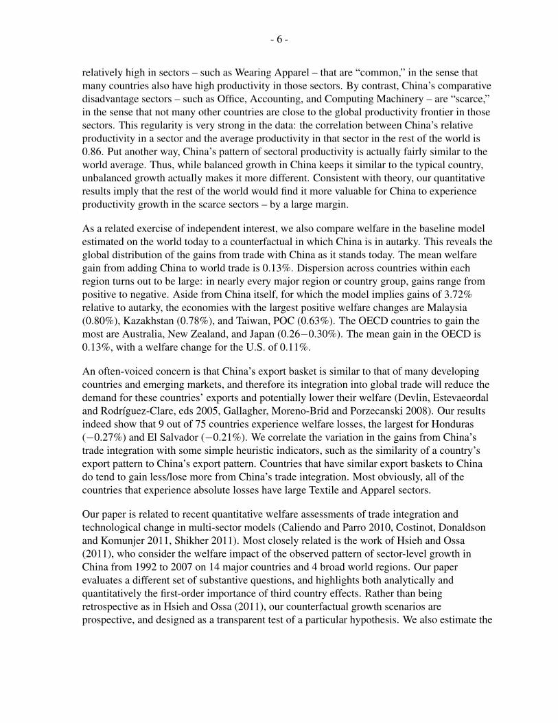
To evaluate the importance of China’s sectoral pattern of growth for global welfare, wesimulate two counterfactual growth scenarios starting from the present day. In the first,China’s productivity growth rate in each sector is identical, and equal to the averageproductivity growth we estimate for China between the 1990s and the 2000s, which is 14%(i.e. an average of 1.32% per annum). In this “balanced” growth scenario, China’scomparative advantage vis-a-vis the world remains unchanged. In the second scenario China’scomparative disadvantage sectors grow disproportionally faster. Specifically, in the“unbalanced” counterfactual China’s relative productivity differences with respect to theworld frontier are eliminated, and China’s productivity in every sector becomes a constantratio of the world frontier. By design, the average productivity in China is the same in the twocounterfactuals. What differs is the relative productivities across sectors.
The results are striking. The mean welfare gains (the percentage change in real consumption)from the unbalanced growth in China, 0.42% in our sample of 74 countries, are some 40 timeslarger than the mean gains in the balanced scenario, which are nearly nil at 0.01%. Thispattern holds for every region and broad country group. Importantly, the large majority ofcountries that become more similar to China in the unbalanced growth scenario – mostprominently the U.S. and the rest of the OECD – still gain much more from unbalancedgrowth in China compared to balanced growth.
Thus, when evaluated quantitatively the welfare impact of China’s growth on the rest of theworld turns out to be the opposite of what had been conjectured by Samuelson (2004). Theanalytical results help us understand why this is the case. What matters is not China’ssimilarity to any individual country, but its similarity to the world weighted averageproductivity (although the theoretically correct weights will differ from country to countrybecause of trade costs). Closer inspection reveals that China’s current productivity is
- 6 -
relatively high in sectors – such as Wearing Apparel – that are “common,” in the sense thatmany countries also have high productivity in those sectors. By contrast, China’s comparativedisadvantage sectors – such as Office, Accounting, and Computing Machinery – are “scarce,”in the sense that not many other countries are close to the global productivity frontier in thosesectors. This regularity is very strong in the data: the correlation between China’s relativeproductivity in a sector and the average productivity in that sector in the rest of the world is0.86. Put another way, China’s pattern of sectoral productivity is actually fairly similar to theworld average. Thus, while balanced growth in China keeps it similar to the typical country,unbalanced growth actually makes it more different. Consistent with theory, our quantitativeresults imply that the rest of the world would find it more valuable for China to experienceproductivity growth in the scarce sectors – by a large margin.
As a related exercise of independent interest, we also compare welfare in the baseline modelestimated on the world today to a counterfactual in which China is in autarky. This reveals theglobal distribution of the gains from trade with China as it stands today. The mean welfaregain from adding China to world trade is 0.13%. Dispersion across countries within eachregion turns out to be large: in nearly every major region or country group, gains range frompositive to negative. Aside from China itself, for which the model implies gains of 3.72%relative to autarky, the economies with the largest positive welfare changes are Malaysia(0.80%), Kazakhstan (0.78%), and Taiwan, POC (0.63%). The OECD countries to gain themost are Australia, New Zealand, and Japan (0.26−0.30%). The mean gain in the OECD is0.13%, with a welfare change for the U.S. of 0.11%.
An often-voiced concern is that China’s export basket is similar to that of many developingcountries and emerging markets, and therefore its integration into global trade will reduce thedemand for these countries’ exports and potentially lower their welfare (Devlin, Estevaeordaland Rodrıguez-Clare, eds 2005, Gallagher, Moreno-Brid and Porzecanski 2008). Our resultsindeed show that 9 out of 75 countries experience welfare losses, the largest for Honduras(−0.27%) and El Salvador (−0.21%). We correlate the variation in the gains from China’strade integration with some simple heuristic indicators, such as the similarity of a country’sexport pattern to China’s export pattern. Countries that have similar export baskets to Chinado tend to gain less/lose more from China’s trade integration. Most obviously, all of thecountries that experience absolute losses have large Textile and Apparel sectors.
Our paper is related to recent quantitative welfare assessments of trade integration andtechnological change in multi-sector models (Caliendo and Parro 2010, Costinot, Donaldsonand Komunjer 2011, Shikher 2011). Most closely related is the work of Hsieh and Ossa(2011), who consider the welfare impact of the observed pattern of sector-level growth inChina from 1992 to 2007 on 14 major countries and 4 broad world regions. Our paperevaluates a different set of substantive questions, and highlights both analytically andquantitatively the first-order importance of third country effects. Rather than beingretrospective as in Hsieh and Ossa (2011), our counterfactual growth scenarios areprospective, and designed as a transparent test of a particular hypothesis. We also estimate the

- 7 -
welfare impact of China’s trade integration to date. Finally, our model has several additionalfeatures important for a reliable quantitative assessment, such as 75 individual countries, aswell as a production structure that includes multiple factors (labor and capital) and the full setof input-output linkages between all sectors. Our work is also related to the ComputableGeneral Equilibrium (CGE) assessments of China’s trade integration (e.g., Francois andWignaraja, 2008, Ghosh and Rao, 2010, Tokarick, 2011). Unlike the traditional CGEapproach, our quantitative framework is based on Eaton and Kortum (2002)’s Ricardianmodel of trade with endogenous specialization both within and across sectors, and the focusof the study is on the role of comparative advantage. Our global general equilibrium approachcomplements recent micro-level studies of the impact of China on developed countries, suchas Autor, Dorn and Hanson (2011) and Bloom, Draca and Van Reenen (2011).
The rest of the paper is organized as follows. Section II derives a set of analytical results usinga simplified multi-sector N -country Eaton and Kortum (2002) model of Ricardian trade.Section III lays out the quantitative framework and describes the details of the calibration.Section IV examines the welfare implications of both the trade integration of China, and thehypothetical scenarios for Chinese growth. Section V performs a set of robustness checks onthe quantitative results. Section VI concludes.
II. ANALYTICAL RESULTS
How will the evolution of relative sectoral technology in a country affect its own welfare andthe welfare of its trading partners? The answer, based on a two-country costless trade modelsuch as the one employed by Samuelson (2004), is that both countries’ welfare is minimizedwhen they have the same relative sectoral productivity. This influential insight must bemodified when we step out of this simple environment and consider more than two countriesand costly trade. This section derives analytical results and builds intuition in a simplifiedversion of the quantitative model of the next section.
In particular, we analyze a multi-sector Eaton and Kortum (2002, henceforth EK) model,proceeding in three steps. We first consider a version of the model in which relative wages inall countries are fixed, and sectoral productivity affects welfare only through the consumptionprice level. This simplification makes analytical results possible, and allows us to demonstratemost simply the role of third countries in how sectoral technological similarity between twotrading partners affects welfare.
Second, we move to the fully general equilibrium case in which changes in relative sectoralproductivity can also affect countries’ relative wages. Because even the simplest multi-sectormodel with more than two countries does not admit an analytical solution in wages, wedemonstrate the results using numerical examples. The essential message of the model isequally strong under endogenous wages. While with 2 countries, welfare is minimized whenrelative sectoral productivity is the same in the two countries, with 3 countries that is nolonger generically the case.

- 8 -
The first two comparative statics are not strictly speaking identical to Samuelson (2004). Theclassic treatment of unbalanced productivity growth assumes that productivity in one sectorrises, while in the other sector it remains unchanged. Thus, there is net productivity growth onaverage in the partner country. By contrast, our first two comparative statics exercisesconsider changes in relative sectoral productivity while keeping the average productivityacross sectors constant. This approach allows for the cleanest statement of the main results,especially under fixed wages, and corresponds precisely to the comparison between our twocounterfactuals, in which we also constrain average productivity to be the same. The third andfinal step of this section presents the numerical results for the classic experiment, in whichone sector’s productivity grows while the other sector’s productivity remains constant,resulting in net average productivity growth in China. The essential result that adding a thirdcountry can reverse the sign of the welfare changes from the same productivity growth isequally true in this experiment.
A. The Environment
There are N countries, indexed by n and i. For concreteness, we can think of country 1 asChina, and evaluate the impact of technological changes in country 1 on itself and country 2,which we can think of as the United States. There are multiple sectors, indexed by j.Production in each sector follows the EK structure. Output Qj
n of sector j in country n is aCES aggregate of a continuum of varieties q = [0, 1] unique to each sector:
Qjn =
[∫ 1
0
Qjn(q)
ε−1ε dq
] εε−1
, (1)
where ε denotes the elasticity of substitution across varieties q, and Qjn(q) is the amount of
variety q that is used in production in sector j and country n.
Producing one unit of good q in sector j in country i requires 1
zji (q)units of labor. Productivity
zji (q) for each q ∈ [0, 1] in each country i and sector j is random, drawn from the Frechetdistribution with cumulative distribution function
F ji (z) = e−T
ji z
−θ. (2)
In this distribution, the absolute advantage term T ji varies by both country and sector, withhigher values of T ji implying higher average productivity draws in sector j in country i. Theparameter θ captures dispersion, with larger values of θ implying smaller dispersion in draws.
Labor is the only factor of production, with country endowments given by Ln and wagesdenoted by wn. The production cost of one unit of good q in sector j and country i is thusequal to wi/z
ji (q). Each country can produce each good in each sector, and international trade
is subject to iceberg costs: djni > 1 units of good q produced in sector j in country i must beshipped to country n in order for one unit to be available for consumption there. The tradecosts need not be symmetric – djni need not equal djin – and will vary by sector. We normalizedjnn = 1 ∀ n and j.
- 9 -
All the product and factor markets are perfectly competitive, and thus the price at whichcountry i can supply tradeable good q in sector j to country n is
pjni(q) =
(wi
zji (q)
)djni.
Buyers of each good q in tradeable sector j in country n will only buy from the cheapestsource country, and thus the price actually paid for this good in country n will be
pjn(q) = mini=1,...,N
{pjni(q)
}. (3)
It is well known that the price of sector j’s output is given by
pjn =
[∫ 1
0
pjn(q)1−εdq
] 11−ε
.
Following the standard EK approach, it is heplful to define
Φjn =
N∑i=1
T ji(wid
jni
)−θ. (4)
This value summarizes, for country n, the access to production technologies in sector j. Itsvalue will be higher if in sector j, country n’s trading partners have high productivity (T ji ) orlow cost (wi). It will also be higher if the trade costs that country n faces in this sector are low.Standard steps (Eaton and Kortum 2002) lead to the familiar result that the price of good j incountry n is simply
pjn = Γ(Φjn
)− 1θ , (5)
where Γ =[Γ(θ+1−εθ
)] 11−ε , with Γ the Gamma function.
Consumer utility is identical across countries and Cobb-Douglas with sector j receivingexpenditure share ηj . The consumption price level in country n is then proportional to
Pn ∝∏j
(pjn)ηj , (6)
and welfare (indirect utility) is given by the real income wn/Pn.
B. Fixed Relative Wages
Consider first the case in which relative wages are fixed. In particular, suppose there are threesectors, j = A,B,H . Sectors A and B have the EK structure described above. As inHelpman, Melitz and Yeaple (2004) and Chaney (2008), good H is homogeneous and can becostlessly traded between any two countries in the world. Let the price of H be the numeraire.
- 10 -
In country n, one worker can produce wn units of H , implying that the wage in n is given bywn. To obtain the cleanest results, let A and B enter symmetrically in the utility function:
Un =(A
12nB
12n
)αH1−αn . (7)
Throughout, we assume that α is sufficiently small so that some amount of H is alwaysproduced in all the countries in the world. This assumption pins down wages in all thecountries, making analytical results possible.
We are now ready to perform the main comparative static: the welfare impact of changes inthe relative technology in country 1, TA1 /T
B1 , subject to the constraint that its geometric
average stays the same:(TA1 T
B1
) 12 = c for some constant c. The exercise informs us of the
welfare impact of the different growth scenarios in China, when we hold its average growthrate fixed.
Lemma 1 Country 1’s relative technology (TA1 /TB1 )n that minimizes welfare in country n
subject to the constraint(TA1 T
B1
) 12
n= c is given by
(TA1TB1
)n
=
∑Ni=2 T
Ai
(wid
Ani
w1dAn1
)−θ∑N
i=2 TBi
(widBniw1dBn1
)−θ . (8)
Proof: See Appendix I.
Lemma 1 says that the country 1 relative technology that minimizes welfare in country n isnot the one that makes country 1 most similar to country n. That is, generically country n’swelfare is not minimized when TA1 /T
B1 = TAn /T
Bn . What matters instead is the
relative-unit-cost-weighted average technologies of all the other countries serving n(including itself). Third countries matter through their technology, but also through theirrelative unit costs and trade costs of serving market n. Because of third country effects, it iseasy to construct examples in which country 1 becomes more technologically similar tocountry n, and yet country n’s welfare increases. Two simple examples under frictionlesstrade can illustrate the point most clearly.
Example 1 Suppose there are two countries and trade is costless. Then the country 1 relativetechnology TA1 /T
B1 that minimizes welfare in countries 1 and 2 is(
TA1TB1
)1
=
(TA1TB1
)2
=TA2TB2
.

- 11 -
Example 2 Suppose there are three countries and trade is costless. Then the country 1relative technology TA1 /T
B1 that minimizes welfare in the three countries is(
TA1TB1
)1
=
(TA1TB1
)2
=
(TA1TB1
)3
=TA2 w
−θ2 + TA3 w
−θ3
TB2 w−θ2 + TB3 w
−θ3
. (9)
In the simple 2-country example the familiar Samuelson (2004) result obtains: both countriesare worst off when TA1 /T
B1 = TA2 /T
B2 . The third country effect is immediate in expression
(9). From the perspective of an individual country, it is generically not the case that in anycountry, welfare is minimized when it is most similar to country 1. In the absence of unitproduction cost differences (w2 = w3), welfare is lowest when country 1 is most similar to thesimple average productivity of countries other than country 1. When unit costs differ, whatmatters for welfare is the production-cost-weighted average, and the lower-wage countrieswill receive a higher weight in this productivity average. Furthermore, as revealed by equation(8), in the presence of trade costs the welfare-minimizing relative productivity is no longer thesame for each country as is the case under frictionless trade.
By comparing the three-country expression in (9) to the N -country case in (8), it is also clearthat as the number of countries increases, the bilateral technological similarity starts to matterless and less, as the weight of the country itself in the summation decreases. As the number ofcountries goes up, for country n’s welfare it becomes more and more important how country 1compares to the countries other than country n rather than to country n itself.
C. Endogenous Wages
The preceding results were derived under the assumption that there is a homogeneouscostlessly traded good and thus the relative wages do not change in response to relativetechnology changes in country 1. The advantage of this approach is that we could obtain themain results analytically even with multiple countries and arbitrary iceberg trade costs, anddemonstrate most clearly the roles of the various simplifying assumptions. The disadvantageis that general equilibrium movements in relative wages could potentially have independenteffects on welfare. Note that as the number of countries increases, the general equilibriumchanges in relative wages in response to technical change in an individual country are likely tobecome smaller and smaller. Nonetheless, it is important to examine whether allowing wagesto adjust in the global trade equilibrium weakens any of the analytical results above.
This subsection implements a 2-sector model in which wages adjust in the global tradeequilibrium. To that end, we remove the homogeneous good from the model: α = 1. Tosimplify the model further, we assume there are no trade costs (djni = 1 ∀j, n, i).Unfortunately, even in the simplest cases, there is no closed-form solution for wages withmore than two countries. We first prove analytically that with 2 countries, thewelfare-minimizing relative productivity has the same form as in Lemma 1 under theseparameter values but now with endogenous wages.
- 12 -
Lemma 2 Let there be 2 countries and 2 tradeable sectors, with utility given by (7) withα = 1. Let there be no international trade costs: djni = 1 ∀j, n, i. Assume TA2 = TB2 = 1 andL1 = L2 = 1. The country 1 relative technology TA1 /T
B1 that minimizes welfare in both
countries subject to the constraint that(TA1 T
B1
) 12 = c is given by
TA1TB1
=TA2TB2
.
Proof: See Appendix I.
In other words, in this special case the result that perfect similarity minimizes welfaregeneralizes to a setting with endogenously determined wages. The key to this outcome is inthe assumptions that the average productivity in both countries is constant as we vary TA1 /T
B1 ,
the two countries have the same size, and trade is costless. As a result, the relative wagesremain constant as the relative sectoral productivity in country 1 changes.
However, we cannot provide a corresponding analytical result with three countries. Thus, wecompare the outcomes under two and three countries using the following numerical example.Country 2’s productivity is the same in the two sectors: TA2 = TB2 = 0.5. Exactly as above,we vary country 1’s relative productivity subject to the constraint that its geometric averageequals 0.5 (the same as in country 2). We solve for wages and welfare in all countriesnumerically for each set of country 1’s relative productivities.
In the two-country case the welfare of both countries as a function of TA1 /TB1 is plotted in
Figure 2(a). As proven analytically, both countries’ welfare is at its lowest point whenTA1 /T
B1 = TA2 /T
B2 = 1. Indeed, only one line is distinguishable in the picture: the welfare of
the two countries is always the same. Next, we introduce a third country of the same size butwith a comparative advantage in sector B: TA3 = 0.25 and TB3 = 1 (so that the geometricaverage productivity in country 3 is the same as in 1 and 2). Figure 2(b) reports the results.Now, no country’s welfare is minimized when TA1 /T
B1 is the same as its relative technology.
Notice that if we start from the right and approach 1 – the point at which TA1 /TB1 = TA2 /T
B2 –
welfare of country 2 actually increases slightly. On the other hand, as we approach 1 from theleft, the welfare of country 1 rises. All in all, it is clear that country 1 becoming more similarto country 2 no longer implies that either country’s welfare falls.
Because the analytical solutions are not available under endogenous wages, we further dissectthe mechanisms behind these welfare results by considering two particular values of country1’s technology parameters, and discussing the behavior of price levels and relative wages. Thetop panel of Table 1 presents the changes in welfare, price levels, and relative wages whenmoving from TA1 /T
B1 = 2 to TA1 /T
B1 = 1.2 Since TA2 /T
B2 = 1, with this technological change
2Welfare in country n is given by wn/P , where P is the consumption price level. Only onechange in P is reported because in this example trade is costless so the consumption pricelevel is the same everywhere.
- 13 -
country 1 becomes more similar (indeed identical) to country 2. The left column presents thewelfare change in the 2-country world. As already shown, greater similarity between the twocountries lowers welfare in both. This effect operates entirely through a rise in theconsumption price level: the relative wage between the countries does not move. The rightcolumn instead presents the results in the 3-country world. The exact same change intechnology in country 1 now raises welfare in country 2. Part of what is happening is that dueto this change in productivity, w3/w2 falls. Thus it appears that in this numerical example,changes in comparative advantage of country 1 lead to a “multilateral relative wage effect:”country 2 gains in welfare over this range partly because technology changes in country 1 leadto cheaper imports from country 3.
Table 1 also reports the changes in sector A net exports as a share of GDP in all the countries(by balanced trade, net exports of sector A and B sum to zero in each country). A greaterabsolute deviation from zero implies a greater degree of inter-industry trade. With 2 countries,as country 1 becomes more similar to country 2 in relative technology, inter-industry tradedisappears entirely: country 2 goes from being a net importer in sector A to balanced tradewithin the sector. With 3 countries, the same exact change in country 1’s technology leads toan increase in inter-industry trade in country 2 (a rise in sector A net exports to GDP from0.05 to 0.11). Thus, just as greater similarity between countries 1 and 2 need not lowercountry 2’s welfare when there are more than 2 countries, greater similarity also need notreduce inter-industry trade.
Finally, we circle all the way back to the original Samuelson (2004) comparative static inwhich productivity grows in country 1’s comparative disadvantage sector, but stays constantin its comparative advantage sector, implying net average productivity growth in country 1 asit becomes more similar to country 2. In this experiment, TA1 = 0.5 throughout, while TB1rises from 0.1 to 0.5. Thus, by design, the end point of this technological change is exactly thesame as in the experiment above: countries 1 and 2 end up identical. The bottom panel ofTable 1 reports the results. With two countries, it is still the case that as country 1 becomesmore similar, country 2 sees absolute welfare losses. Here, the mechanics for the effect aresomewhat distinct. While the consumption price level expressed relative to the numeraire –the wage of country 1 – falls, country 2’s relative wage falls by more, precipitating welfarelosses. By contrast, with three countries, the same change in country 1’s technology leads towelfare gains for country 2. Again, part of what is happening is that w3/w2 falls, leading tocheaper imports from country 3. Inter-industry trade in country 2 also rises in this experiment.
We conclude from both the analytical results with fixed wages, and the numerical exampleswith endogenous wages, that third country effects are of first-order importance for evaluatingthe impact of changes in relative technology in one country on itself and its trading partners.Before moving on to the quantitative analysis, it is worth mentioning the relationship betweenour results and a common interpretation that the mechanism in the Samuelson (2004)-typeresult operates through the terms of trade. In the 2× 2 first-generation Ricardian model, termsof trade are isomorphic to welfare. The easiest way to see this is to suppose that utility is
- 14 -
Cobb-Douglas in two symmetric sectors A and B, country 1 produces A with productivityz1A, while country 2 produces B with productivity z2B. Then, welfare – indirect utility – incountry 2 is given by w2/P2 = w2/(w2z2Bw1z1A)1/2 = (w2/w1)
1/2(z2Bz1A)−1/2. The termsof trade, on the other hand, are equal to (w2/w1)(z2B/z1A). Thus, as long as z2B and z1A areunchanged – as was the case in the comparative static considered by Samuelson (2004) – theterms of trade are the same as welfare up to a constant. This equivalence may be helpful tobuild intuition but it breaks down in more sophisticated models such as EK, where it is nolonger the case that the terms of trade are isomorphic to welfare. The conceptually correctobject of analysis is indirect utility rather than the terms of trade.
III. QUANTITATIVE FRAMEWORK
To evaluate quantitatively the global welfare impact of balanced and unbalanced sectoralproductivity growth in China, we build on the conceptual framework and results above in tworespects. First, we enrich the model in a number of dimensions to make it suitable forquantitative analysis. Relative to the simple model in Section II, the complete quantitativeframework features (i) multiple factors of production – capital and labor; (ii) an explicitnontradeable sector; (iii) input-output linkages between all sectors; (iv) CES aggregation oftradeable consumption goods, with taste differences across goods. Second, we requiresectoral productivity estimates (T jn) for a large number of countries and sectors in the world.Sectoral productivities are obtained from Levchenko and Zhang (2011), which extends theapproach of Eaton and Kortum (2002) and uses bilateral trade data at sector level combinedwith a model-implied gravity relationship to estimate sector-level productivities. Thequantitative framework is implemented on a sample of 75 countries, which in addition toChina includes countries from all continents and major world regions.
A. The Environment
There are n, i = 1, ..., N countries, J tradeable sectors, and one nontradeable sector J + 1.Utility over the sectors in country n is given by
Un =
(J∑j=1
ω1η
j
(Y jn
) η−1η
) ηη−1
ξn (Y J+1n
)1−ξn, (10)
where ξn denotes the Cobb-Douglas weight for the tradeable sector composite good, η is theelasticity of substitution between the tradeable sectors, Y J+1
n is final consumption of thenontradeable-sector composite good, and Y j
n is the final consumption of the composite goodin tradeable sector j. Importantly, while Section II relied on Cobb-Douglas preferences andsymmetry of the tradeable sectors in the utility function, the quantitative model adopts CESpreferences and allows ωj – the taste parameter for tradeable sector j – to differ across sectors.
As in Section II, output in sector j aggregates a continuum of varieties q ∈ [0, 1] according toequation (1), and the unit input requirement 1
zji (q)for variety q is drawn from the country- and
sector-specific productivity distribution given by equation (2). Production uses labor, capital,
- 15 -
and intermediate inputs from other sectors. The cost of an input bundle in country i is
cji =(wαji r
1−αji
)βj (J+1∏k=1
(pki)γk,j)1−βj
,
where wi is the wage, ri is the return to capital, and pki is the price of intermediate input fromsector k. The value-added based labor intensity is given by αj , and the share of value added intotal output by βj . Both vary by sector. The shares of inputs from other sectors γk,j vary byoutput industry j as well as input industry k. The production cost of one unit of good q insector j and country n is thus equal to cji/z
ji (q), and the price at which country i can serve
market n is pjni(q) =(
cjizji (q)
)djni. The price pjn(q) that country n actually pays for good q is
given by equation (3).
B. Characterization of Equilibrium
The competitive equilibrium of this model world economy consists of a set of prices,allocation rules, and trade shares such that (i) given the prices, all firms’ inputs satisfy thefirst-order conditions, and their output is given by the production function; (ii) given theprices, the consumers’ demand satisfies the first-order conditions; (iii) the prices ensure themarket clearing conditions for labor, capital, tradeable goods and nontradeable goods; (iv)trade shares ensure balanced trade for each country.3
The set of prices includes the wage rate wn, the rental rate rn, the sectoral prices {pjn}J+1j=1 , and
the aggregate price Pn in each country n. The allocation rules include the capital and laborallocation across sectors {Kj
n, Ljn}J+1
j=1 , final consumption demand {Y jn }J+1
j=1 , and total demand{Qj
n}J+1j=1 (both final and intermediate goods) for each sector. The trade shares include the
expenditure share πjni in country n on goods coming from country i in sector j.
Demand and Prices
The price of sector j output in country n is given by equations (4) and (5), with the onlydifference that the expression for Φj
n in equation (4) features cji instead of wi. Theconsumption price index in country n is then
Pn = Bn
(J∑j=1
ωj(pjn)1−η
) 11−η ξn
(pJ+1n )1−ξn , (11)
where Bn = ξ−ξnn (1− ξn)−(1−ξn).
3The assumption of balanced trade is not crucial for the results. Section A implements amodel with unbalanced trade following the approach of Dekle, Eaton and Kortum(2007, 2008), and shows that the conclusions are quite similar.
- 16 -
Both capital and labor are mobile across sectors and immobile across countries, and trade isbalanced. The budget constraint (or the resource constraint) of the consumer is thus given by
J+1∑j=1
pjnYjn = wnLn + rnKn, (12)
where Kn and Ln are the endowments of capital and labor in country n.
Given the set of prices {wn, rn, Pn, {pjn}J+1j=1 }Nn=1, we first characterize the optimal allocations
from final demand. Consumers maximize utility (10) subject to the budget constraint (12).The first order conditions associated with this optimization problem imply the following finaldemand:
pjnYjn = ξn(wnLn + rnKn)
ωj(pjn)1−η∑J
k=1 ωk(pkn)1−η
, for all j = {1, .., J} (13)
andpJ+1n Y J+1
n = (1− ξn)(wnLn + rnKn).
Production Allocation and Market Clearing
The EK structure in each sector j delivers the standard result that the probability of importinggood q from country i, πjni, is equal to the share of total spending on goods coming fromcountry i, Xj
ni/Xjn, and is given by
Xjni
Xjn
= πjni =T ji(cjid
jni
)−θΦjn
.
Let Qjn denote the total sectoral demand in country n and sector j. Qj
n is used for both finalconsumption and intermediate inputs in domestic production of all sectors. That is,
pjnQjn = pjnY
jn +
J∑k=1
(1− βk)γj,k
(N∑i=1
πkinpkiQ
ki
)+ (1− βJ+1)γj,J+1p
J+1n QJ+1
n
for tradeable sectors j = 1, ..., J , and
pJ+1n QJ+1
n = pJ+1n Y J+1
n +J+1∑k=1
(1− βk)γj,kpknQkn
in the nontradeable sector. That is, total expenditure in sector j = 1, ..., J of country n, pjnQjn,
is the sum of (i) domestic final consumption expenditure pjnYjn ; (ii) expenditure on sector j
goods as intermediate inputs in all the traded sectors∑J
k=1(1− βk)γj,k(∑N
i=1 πkinp
kiQ
ki ), and
(iii) expenditure on the j’s sector intermediate inputs in the domestic non-traded sector(1− βJ+1)γj,J+1p
J+1n QJ+1
n . These market clearing conditions summarize the two importantfeatures of the world economy captured by our model: complex international production

- 17 -
linkages, as much of world trade is in intermediate inputs, and a good crosses borders multipletimes before being consumed (Hummels, Ishii and Yi 2001); and two-way input linkagesbetween the tradeable and the nontradeable sectors.
In each tradeable sector j, some goods q are imported from abroad and some goods q areexported to the rest of the world. Country n’s exports in sector j are given byEXj
n =∑N
i=1 1Ii6=nπjinp
jiQ
ji , and its imports in sector j are given by
IM jn =
∑Ni=1 1Ii6=nπ
jnip
jnQ
jn, where 1Ii6=n is the indicator function. The total exports of country
n are then EXn =∑J
j=1EXjn, and total imports are IMn =
∑Jj=1 IM
jn. Trade balance
requires that for any country n, EXn − IMn = 0.
Given the total production revenue in tradeable sector j in country n,∑N
i=1 πjinp
jiQ
ji , the
optimal sectoral factor allocations must satisfy
N∑i=1
πjinpjiQ
ji =
wnLjn
αjβj=
rnKjn
(1− αj)βj.
For the nontradeable sector J + 1, the optimal factor allocations in country n are simply givenby
pJ+1n QJ+1
n =wnL
J+1n
αJ+1βJ+1
=rnK
J+1n
(1− αJ+1)βJ+1
.
Finally, for any n the feasibility conditions for factors are given by
J+1∑j=1
Ljn = Ln andJ+1∑j=1
Kjn = Kn.
C. Welfare
Welfare in this framework corresponds to the indirect utility function. Straightforward stepsusing the CES functional form can be used to show that the indirect utility in each country nis equal to total income divided by the price level. Since both goods and factor markets arecompetitive, total income equals the total returns to factors of production. Thus total welfarein a country is given by (wnLn + rnKn) /Pn, where the consumption price level Pn comesfrom equation (11). Expressed in per-capita terms it becomes
wn + rnknPn
, (14)
where kn = Kn/Ln is capital per worker. This expression is the metric of welfare in allcounterfactual exercises below.
D. Calibration
In order to implement the model numerically, we must calibrate the following sets ofparameters: (i) moments of the productivity distributions T jn and θ; (ii) trade costs djni; (iii)
- 18 -
production function parameters αj , βj , γk,j , and ε; (iv) country factor endowments Ln andKn; and (v) preference parameters ξn, ωj , and η. We discuss the calibration of each in turn.
The structure of the model is used to estimate many of its parameters, most importantly thesector-level technology parameters T jn for a large set of countries. The first step, most relevantto this study, is to estimate the technology parameters in the tradeable sectors relative to areference country (the U.S.) using data on sectoral output and bilateral trade. The procedurerelies on fitting a structural gravity equation implied by the model, and using the resultingestimates along with data on input costs to back out underlying technology. Intuitively, ifcontrolling for the typical gravity determinants of trade, a country spends relatively more ondomestically produced goods in a particular sector, it is revealed to have either a high relativeproductivity or a low relative unit cost in that sector. The procedure then uses data on factorand intermediate input prices to net out the role of factor costs, yielding an estimate of relativeproductivity. This step also produces estimates of bilateral sector-level trade costs djni. Theparametric model for iceberg trade costs includes the common geographic variables such asdistance and common border, as well as policy variables, such as regional trade agreementsand currency unions.
The second step is to estimate the technology parameters in the tradeable sectors for the U.S..This procedure requires directly measuring TFP at the sectoral level using data on real outputand inputs, and then correcting measured TFP for selection due to trade. The taste parametersfor all tradeable sectors ωj are also calibrated in this step. The third step is to calibrate thenontradeable technology for all countries using the first-order condition of the model and therelative prices of nontradeables observed in the data. The detailed procedures for all threesteps are described in Levchenko and Zhang (2011) and reproduced in Appendix II.
We assume that the dispersion parameter θ does not vary across sectors. There are no reliableestimates of how it varies across sectors, and thus we do not model this variation. We pick thevalue of θ = 8.28, which is the preferred estimate of EK.4 It is important to assess how theresults below are affected by the value of this parameter. One may be especially concernedabout how the results change under lower values of θ. Lower θ implies greater within-sectorheterogeneity in the random productivity draws. Thus, trade flows become less sensitive to thecosts of the input bundles (cji ), and the gains from intra-sectoral trade become larger relativeto the gains from inter-sectoral trade. Elsewhere (Levchenko and Zhang 2011) we
4Shikher (2004, 2005, 2011), Burstein and Vogel (2009), and Eaton, Kortum, Neiman andRomalis (2010), among others, follow the same approach of assuming the same θ acrosssectors. Caliendo and Parro (2010) use tariff data and triple differencing to estimatesector-level θ. However, their approach may suffer from significant measurement error: attimes the values of θ they estimate are negative. In addition, in each sector the restriction thatθ > ε− 1 must be satisfied, and it is not clear whether Caliendo and Parro (2010)’s estimatedsectoral θ’s meet this restriction in every case. Our approach is thus conservative by beingagnostic on this variation across sectors.

- 19 -
re-estimated all the technology parameters using instead a value of θ = 4, which has beenadvocated by Simonovska and Waugh (2010) and is at or near the bottom of the range that hasbeen used in the literature. Overall, the outcome was remarkably similar. The correlationbetween estimated T ji ’s under θ = 4 and the baseline is above 0.95, and there is actuallysomewhat greater variability in T ji ’s under θ = 4.
The production function parameters αj and βj are estimated using the UNIDO IndustrialStatistics Database, which reports output, value added, employment, and wage bills at theroughly 2-digit ISIC Revision 3 level of disaggregation. To compute αj for each sector, wecalculate the share of the total wage bill in value added, and take a simple median acrosscountries (taking the mean yields essentially the same results). To compute βj , we take themedian of value added divided by total output.
The intermediate input coefficients γk,j are obtained from the Direct Requirements Table forthe United States. We use the 1997 Benchmark Detailed Make and Use Tables (coveringapproximately 500 distinct sectors), as well as a concordance to the ISIC Revision 3classification to build a Direct Requirements Table at the 2-digit ISIC level. The DirectRequirements Table gives the value of the intermediate input in row k required to produce onedollar of final output in column j. Thus, it is the direct counterpart to the input coefficientsγk,j . Note that we assume these to be the same in all countries.5 In addition, we use the U.S.I-O matrix to obtain αJ+1 and βJ+1 in the nontradeable sector, which cannot be obtained fromUNIDO.6 The elasticity of substitution between varieties within each tradeable sector, ε, is setto 4.
The total labor force in each country, Ln, and the total capital stock, Kn, are obtained from thePenn World Tables 6.3. Following the standard approach in the literature (see, e.g., Hall andJones, 1999, Bernanke and Gurkaynak, 2001, Caselli, 2005), the total labor force is calculatedfrom the data on the total GDP per capita and per worker.7 The total capital is calculated using
5di Giovanni and Levchenko (2010) provide suggestive evidence that at such a coarse level ofaggregation, Input-Output matrices are indeed similar across countries. To check robustnessof the results, we collected country-specific I-O matrices from the GTAP database.Productivities computed based on country-specific I-O matrices were very similar to thebaseline values. In our sample of countries, the median correlation was 0.98, with all but 3 outof 75 countries having a correlation of 0.93 or above, and the minimum correlation of 0.65.
6The U.S. I-O matrix provides an alternative way of computing αj and βj . These parameterscalculated based on the U.S. I-O table are very similar to those obtained from UNIDO, withthe correlation coefficients between them above 0.85 in each case. The U.S. I-O table impliesgreater variability in αj’s and βj’s across sectors than does UNIDO.
7Using the variable name conventions in the Penn World Tables,Ln = 1000 ∗ pop ∗ rgdpch/rgdpwok.
- 20 -
the perpetual inventory method that assumes a depreciation rate of 6%:Kn,t = (1− 0.06)Kn,t−1 + In,t, where In,t is total investment in country n in period t. Formost countries, investment data start in 1950, and the initial value of Kn is set equal toIn,0/(γ + 0.06), where γ is the average growth rate of investment in the first 10 years forwhich data are available.
The share of expenditure on traded goods, ξn in each country is sourced from Yi and Zhang(2010), who compile this information for 36 developed and developing countries. Forcountries unavailable in the Yi and Zhang data, values of ξn are imputed based their level ofdevelopment. We fit a simple linear relationship between ξn and log PPP-adjusted per capitaGDP from the Penn World Tables on the countries in the Yi and Zhang (2010) dataset. The fitof this simple bivariate linear relationship is quite good, with an R2 of 0.55. For the remainingcountries, we then set ξn to the value predicted by this bivariate regression at their level ofincome. The taste parameters for tradeable sectors ωj were estimated by combining the modelstructure above with data on final consumption expenditure shares in the U.S. sourced fromthe U.S. Input-Output matrix, as described in Appendix II. The elasticity of substitutionbetween broad sectors within the tradeable bundle, η, is set to 2. Since these are very largeproduct categories, it is sensible that this elasticity would be relatively low. It is higher,however, than the elasticity of substitution between tradeable and nontradeable goods, whichis set to 1 by the Cobb-Douglas assumption.
E. Summary of the Estimates and Basic Patterns
All of the variables that vary over time are averaged for the period 2000-2007 (the latestavailable year), which is the time period on which we carry out the analysis. Appendix TableA1 lists the 75 countries used in the analysis, separating them into the major country groupsand regions. Appendix Table A2 lists the 20 sectors along with the key parameter values foreach sector: αj , βj , the share of nontradeable inputs in total inputs γJ+1,j , and the tasteparameter ωj .
Countries differ markedly with respect to their trade relationship with China. The top panel ofTable 2 lists the top 10 and bottom 10 countries in terms of the average trade costs (djni) withChina, while the bottom panel reports the top 10 and bottom 10 countries in terms of thecorrelation between the tradeable sector productivities with China. Since average sectoralproductivity scales with (T jn)1/θ rather than T jn, and since we want to focus on differences incomparative rather than absolute advantage, we compute the correlations on the vectors of(T jn)1/θ demeaned by each country’s geometric average of those sectoral productivities.
Average trade costs vary from 1.6–1.7 for Japan, Korea and United States, to 3.95 for Trinidadand Tobago and Ethiopia. Not surprisingly, the trade costs implied by our model correlatepositively with distance, with the countries in Asia as the ones with lowest trade costs, thoughnot without exception: the U.S., the U.K, and Germany are in the bottom 10. Technologicalsimilarity varies a great deal as well, from correlations in excess of 0.9 with India, Turkey, andIndonesia, to correlations below 0.6 with Sri Lanka, Bolivia, and Iceland. It is clear that the
- 21 -
regional component is not as prevalent here, with both most similar and most differentcountries drawn from different parts of the world.
IV. WELFARE ANALYSIS
This section analyzes the global welfare impact of China’s trade integration and variousproductivity growth scenarios. We proceed by first solving the model under the baselinevalues of all the estimated parameters, and present a number of checks on the model fit withrespect to observed data. Then, we compute counterfactual welfare under two main sets ofexperiments. The first assumes that China is in autarky, and is intended to give a measure ofthe worldwide gains from trade with China. The second instead starts from today’sequilibrium, and evaluates the implications of alternative patterns of China’s productivitygrowth going forward. The model solution algorithm is described in Levchenko and Zhang(2011).
A. Model Fit
Table 3 compares the wages, returns to capital, and the trade shares in the baseline modelsolution and in the data. The top panel shows that mean and median wages implied by themodel are very close to the data. The correlation coefficient between model-implied wagesand those in the data is above 0.99. The second panel performs the same comparison for thereturn to capital. Since it is difficult to observe the return to capital in the data, we follow theapproach adopted in the estimation of T jn’s and impute rn from an aggregate factor marketclearing condition: rn/wn = (1− α)Ln/ (αKn), where α is the aggregate share of labor inGDP, assumed to be 2/3. Once again, the average levels of rn are very similar in the modeland the data, and the correlation between the two is in excess of 0.95.
Next, we compare the trade shares implied by the model to those in the data. The third panelof Table 3 reports the spending on domestically produced goods as a share of overallspending, πjnn. These values reflect the overall trade openness, with lower values implyinghigher international trade as a share of absorption. Though we under-predict overall tradeslightly (model πjnn’s tend to be higher), the averages are quite similar, and the correlationbetween the model and data values is 0.91. Finally, the bottom panel compares theinternational trade flows in the model and the data. The averages are very close, and thecorrelation between model and data is 0.9.
Figure 3 presents the comparison of trade flows graphically, by depicting the model-impliedtrade values against the data, along with a 45-degree line. Red/solid dots indicate πjni’s thatinvolve China, that is, trade flows in which China is either an exporter or an importer. All inall the fit of the model to trade flows is quite good. China is unexceptional, with Chinese flowsclustered together with the rest of the observations.
We conclude from this exercise that our model matches quite closely the relative incomes ofcountries as well as bilateral and overall trade flows observed in the data. We now use the
- 22 -
model to carry out the two counterfactual scenarios. One captures the gains from trade withChina as it stands now. The other considers two possible growth patterns for China.
B. Gains from Trade with China
Panel A of Table 4 reports the gains from trade with China around the world. To computethese, we compare welfare of each country in the baseline (current levels of trade costs andproductivities as we estimate them in the world today) against a counterfactual scenario inwhich China is in autarky. The table reports the change in welfare for China itself, as well asthe summary statistics for each region and country group. China’s gains from trade relative tocomplete autarky are 3.72%. Elsewhere in the world, the gains range from −0.27% to 0.80%,with the mean of 0.13%.8 The gains for the rest of the world from China’s trade integrationare smaller than for China itself because these gains are relative to the counterfactual thatpreserves all the global trade relationships other than with China.
The countries gaining the most tend to be close to China geographically: Malaysia (0.80%),Kazakhstan (0.78%), and Taiwan, POC (0.63%). Of the top 10, 7 are in Asia, and theremaining three are Peru (0.39%), Chile (0.37%), and Australia (0.30%). The OECDcountries to gain the most are Australia, New Zealand, and Japan at 0.26%−0.30%. The meangain in the OECD is 0.13%, and the welfare change for the U.S. is 0.11%. Table 4 also revealsthat in nearly every major country group, the welfare changes range from negative to positive.The countries to lose the most from entry of China into world trade are Honduras (−0.27%)and El Salvador (−21%). All in all, 9 out of 75 countries experience negative welfarechanges. By and large, countries that lose tend to be producers of Textiles and Apparel: SriLanka, Bulgaria, Vietnam, Mauritius, and Portugal are all among the losing countries.
Our multi-country multi-sector model does not admit an analytical expression for themagnitude of the gains from trade with China, as those gains depend on all the parameterscharacterizing the country and all of its trading partners. Nonetheless, we investigate whetherthe variation in the gains from trade with China across countries can be explained – in theleast-squares sense – by three simple measures of countries’ multilateral trade linkages withChina. The first is the correlation between a country’s export shares and China’s exportshares. This measure is meant to capture the extent to which China competes with the countryin world product markets. A high correlation means that the country has a very similar exportbasket to China, and thus will compete with it head-to-head. All else equal, we would expectcountries with a higher correlation to experience smaller gains from integration of China.
8This is the unweighted mean across the 74 countries. The population-weighted mean is veryclose at 0.12%. One may also be interested in comparing the gains from trade with China toother commonly calculated magnitudes in these types of models, such as the total gains fromtrade. Elsewhere (Levchenko and Zhang 2011) we report that the median gain from trade inthis type of model among these 75 countries is 4.5%, with the range from 0.5% to 12.2%.
- 23 -
The second measure is the correlation between a country’s export shares and China’s importshares. This indicator is meant to reflect China’s demand for the goods that the countryexports. If the correlation is high, this means China imports a lot of the goods that the countryexports, and thus all else equal the country’s gains from introducing China into the worldeconomy should be higher. Finally, the last indicator is the correlation between China’s exportshares and the country’s import shares. It is meant to measure the extent to which a countryvalues the goods produced by China: a high correlation means that the country imports a lotof the goods that China exports, which should lead to greater gains, ceteris paribus.
In our sample of countries, we regress gains from integration of China on these three heuristicindicators, controlling for the (log) average djni between the country and China, and (log)country population.9 The overall R2 in this regression is 0.38. All three are significant andhave the expected sign. It is important to emphasize that we do not seek any kind of causalinterpretation in this exercise. Instead, the goal is only to find some simple and intuitiveindicators that can account for some of the cross-country variation in gains. With that caveat,Figure 4 depicts the partial correlations between the three indicators of interest and thewelfare gains from China’s integration. The top panel shows that countries with similar exportbaskets to China tend to gain less. The relationship is highly significant, with a t-statistic ofnearly 4. The middle panel illustrates that countries that export goods imported by China tendto benefit more. The relationship is once again highly significant, with a t-statistic of 4.Finally, the bottom panel shows that countries whose import basket is similar to China’sexport basket tend to gain more. The relationship is less strong than the other two, but stillsignificant at the 5% level. We conclude from this exercise that the gains from trade withChina are well explained by some simple heuristic measures of head-to-head competition withChina in world markets, Chinese demand for a country’s goods, and Chinese supply of thegoods that a country imports.
C. Balanced and Unbalanced Growth
The preceding counterfactual was with respect to trade costs: it assumed that trade costs facedby China were prohibitive, and thus it was in autarky. The conjecture put forward bySamuelson (2004) is about uneven technical change in China going forward: given theprevailing level of trade costs, global welfare will be affected differently depending on thepattern of sectoral productivity growth in China.
To evaluate Samuelson’s conjecture, we simulate two productivity growth scenarios startingfrom today’s values of China’s T jn’s. Figure 5 depicts these two counterfactuals graphically.The solid dots, labelled by the sector number, represent the actual ratio of productivity to theglobal frontier in each sector in China in the 2000s. We can see that the comparativeadvantage sectors are Coke, Refined Petroleum Products, Nuclear Fuel; Wearing Apparel; and
9All the results are unchanged if we use total country GDP instead of population as a measureof size, or if we use levels of djni and population or GDP instead of logs.

- 24 -
Transport Equipment. The productivity of these sectors is about 0.45−0.5 of the worldfrontier productivity. The sectors at the greatest comparative disadvantage are Printing andPublishing; Office, Accounting, Computing, and Other Machinery; and Medical, Precision,and Optical Instruments. The productivity of these sectors is around 0.25 of the world frontier.The solid line denotes the geometric average of China’s productivity as a ratio to the worldfrontier productivity in the 2000s, which is about 0.34.10
The two counterfactual productivity scenarios are plotted in the figure. In the balanced growthscenario, we assume that in each sector China’s distance to the global frontier has grown bythe same proportional rate of 14% (or 1.32% per annum), which is the observed growth ofaverage T jn’s in China relative to the world frontier over a decade between the 1990s and the2000s. The balanced counterfactual productivities are depicted by the hollow dots. In theunbalanced growth counterfactual, we assume that China’s average productivity grows by thesame rate, but its comparative advantage relative to world frontier is erased: in each sector, itsproductivity is a constant fraction of world frontier. That scenario is depicted by the hollowtriangles. An attractive feature of this setup is that in the two counterfactuals, the geometricaverage productivity across sectors in China is the same. The only thing that is different is thecomparative advantage.11
Panels B and C of Table 5 present the results for the balanced and the unbalancedcounterfactuals, respectively. The results are striking. The rest of the world gains much morefrom unbalanced growth in China. The difference is of an order of magnitude or more. Whilemean and median gains from balanced growth for the OECD are 0.01–0.02%, they are0.12–0.17% in the unbalanced growth case. For other regions the difference is even larger:0.23–0.84% at the mean in the unbalanced case, compared to essentially zero in the balancedcase.12 Figure 6(a) presents the contrast between the the welfare changes in the twocounterfactual scenarios graphically, by plotting the welfare changes in each country in thebalanced case on the y-axis against the welfare changes in the unbalanced case on the x-axis,along with a 45-degree line. While there is a great deal of variation in the welfare changesunder the unbalanced case, the balanced counterfactual welfare changes are all very close to
10Since mean productivity in each sector is equal to T 1/θ, the figure reports the distance to theglobal frontier expressed in terms of T 1/θ, rather than T .
11We keep productivity in the nontradeable sector at the benchmark value in all thecounterfactual experiments, since our focus is on the welfare impact of changes incomparative advantage.
12Once again, while we report the simple means across countries throughout,population-weighted averages turn out to be very similar. In the sample of 74 countries, underthe balanced counterfactual both unweighted and population-weighted mean welfare changesare 0.01%. In the unbalanced counterfactual, the unweighted mean welfare change is 0.42%,compared to the population-weighted average of 0.39%.

- 25 -
zero. In the large majority of cases, the observation is well below the 45-degree line: thecountry gains more in the unbalanced counterfactual.
These results are diametrically opposite to what has been conjectured by Samuelson (2004),who feared that China’s growth in its comparative disadvantage sectors will hurt the rest ofthe world. We devote the rest of this section to exploring in detail the mechanisms behind thisfinding. The analytical section derives the multilateral similarity effect in a simple model withexogenously fixed wages. To isolate the channel emphasized by the analytical results, as anintermediate step we compute an alternative change in welfare under the assumption that wand r do not change from their baseline values.13 Doing so allows us to focus on the changesin the price levels driven purely by changes in technology parameters rather than relativefactor prices. Figure 6(b) presents a scatterplot of the welfare changes in the balancedcounterfactual against the welfare changes in the unbalanced one under fixed factor prices.The essential result that the world gains much more from unbalanced growth in China stillobtains when factor prices do not change. The mechanism highlighted in the analyticalsection clearly contributes to generating the quantitative results.
As demonstrated in Section II, what matters for an individual country is how China’stechnology compares not to itself, but to appropriately averaged world productivity. Figure 7plots China’s distance to the global frontier in each sector against the simple average of thedistance to the global frontier in all the countries in the sample except China, along with theleast-squares fit. The world average distance to the frontier captures in a simple way howproductive countries are on average in each sector. Higher values imply that the world as awhole is fairly productive in those sectors. Lower values imply that the world is fairlyunproductive in those sectors.
The relationship is striking: China’s comparative advantage sectors are also the ones in whichother countries tend to be more productive. The simple correlation between these twovariables is a remarkable 0.86.14 Thus, China’s comparative advantage is in “common”sectors, those in which many other countries are already productive, most obviously WearingApparel. By contrast, China’s comparative disadvantage is in “scarce” sectors in which notmany countries are productive, for example Medical, Precision, and Optical Instruments.Thus, it is more valuable for the world if China improves productivity in the globally scarcesectors.
13Note that this of course does not involve a solution to the model, and these values do notcorrespond to any actual equilibrium. They are simply the hypothetical values of the changein the welfare expression (14) that obtain when wn and rn remain at their baseline values butT jn’s for China change to their counterfactual values.
14The plot and the reported correlation drop Tobacco, which is a small sector and an outlier.With Tobacco, the correlation is 0.78.

- 26 -
Having isolated the impact of multilateral similarity by fixing w and r, we next explore therole of endogenous factor prices. Figure 8 plots the welfare change under endogenous w and ron the y-axis against the welfare change under fixed w and r on the x-axis. Panel (a) reportsthe scatterplot for the balanced counterfactual, while panel (b) for the unbalancedcounterfactual. Several things stand out about the role of endogenous factor prices. First, inall countries (of course, except China) and both counterfactuals, the gains are larger underfixed factor prices. This is not surprising: when factor prices are fixed, the technologicalimprovement in China is not accompanied by rising factor costs, giving all the countriesexcept China a benefit of better technology without the cost of higher Chinese wages andreturns to capital.
Second, in the balanced counterfactual, from the perspective of almost every country, thebenefit from better Chinese technology is essentially perfectly cancelled out by the higherfactor prices in China. While there is some dispersion in how much countries gain under fixedfactor prices (from zero to 2%), that dispersion disappears when factor prices are allowed toadjust. Countries that gain more from better Chinese technology when w and r are fixed alsolose more from higher w and r in China, such that the net gains to them are nil.
Third, the counteracting movements in w and r are weaker in the unbalanced counterfactual.In contrast to the balanced growth case, it is not generally the case that the benefits tocountries from Chinese technological change are perfectly undone by movements in factorprices. That off-setting effect exists, but it is much less strong. There is a clear positiverelationship between welfare gains under fixed factor prices and gains with flexible ones:countries that gain the most from changes in Chinese technology when factor prices are fixedcontinue to gain more when factor prices adjust. Thus, there is an additional effect ofunbalanced growth that works through endogenous factor prices: compared to balancedgrowth, Chinese relative factor prices do not rise as much, and thus wipe out less of the gainsto other countries from average productivity increases in China.
Next we explore technological similarity as a determinant of the gains from unbalancedgrowth in China. Figure 9(a) plots the welfare change in the unbalanced counterfactualagainst the simple change in the correlation of T ’s between the country and China. In otherwords, unbalanced growth in China makes China less technologically similar to the countriesbelow zero on the x-axis, and more similar to the countries above zero on the x-axis. Thefigure also depicts the OLS fit through the data. The relationship is negative and verysignificant: in this bivariate regression, the R2 is 0.3 and the robust t-statistic on the change intechnological similarity variable is 5. Countries that become more similar to China as a resultof China’s unbalanced growth thus tend to gain less from that growth. (Note that as shown inFigure 6(a), nearly all countries, including ones that become more similar to China,nonetheless gain more from unbalanced growth compared to the balanced one.)
There could be two explanations for this robust negative correlation. The first is that whenChina becomes more similar, demand for the country’s output goes down, pushing downfactor prices. As a result, the country would gain less. The second explanation is about how

- 27 -
trade costs affect multilateral similarity. Equation (8) shows that in the presence of trade costs,TAn and TBn will get a larger weight in the right-hand side expression for country n. That is,when djni’s are substantial, country n’s similarity with China matters more than China’ssimilarity to some other country i. The multilateral similarity effect is still of first-orderimportance in explaining the difference between the balanced and unbalanced growthoutcomes. But when examining the variation in welfare gains across countries under theunbalanced counterfactual, the changes in bilateral technological similarity with Chinabecome relevant. To isolate the second effect, Figure 9(b) relates changes in technologicalsimilarity to welfare changes in the unbalanced counterfactual but this time under fixed factorprices. The strength of the negative relationship is the same: both the R2 and the t-statistic onthe coefficient are virtually identical to the plot with endogenous wages. We conclude that thenegative relationship in Figure 9(a) is not due purely to movements in factor prices.
Finally, China itself gains slightly more from a balanced growth scenario than fromunbalanced growth, 11.43% compared to 10.57%, a difference of almost a percentage point.This result is driven by uneven consumption weights across sectors. It turns out that Chinesesectoral productivity today is strongly positively correlated with the sectoral taste parameterωj , with a correlation of nearly 0.5. In a world characterized by high trade costs, a countrywould be better off with higher productivity in sectors with high taste parameters, all elseequal. In the unbalanced counterfactual, China’s productivity in high-consumption-weightsectors becomes relatively lower.
V. ROBUSTNESS
This section presents a number of robustness checks on the main results. We describe theresults of (i) incorporating trade imbalances; (ii) adding non-manufacturing production andtrade; (iii) using directly measured productivities in countries where they are available; and(iv) considering alternative specifications of the unbalanced counterfactual.
A. Trade Imbalances
One aspect of Chinese trade that has receives a lot of attention is its large surpluses in goodstrade. Trade surpluses result from dynamic decisions, whereas our model is static in nature. Inthe absence of a working model that explains trade imbalances, we incorporate the impact oftrade imbalances following the approach of Dekle, Eaton and Kortum (2007, 2008) andassuming that at a point in time, a trade imbalance represents a transfer from the surplus to thedeficit country. Specifically, the budget constraint (or the resource constraint) of the consumeris now
J+1∑j=1
pjnYjn = wnLn + rnKn −Dn,
where Dn is the trade surplus of country n. When Dn is negative, countries are running adeficit and consume more than their factor income. The deficits add up to zero globally,∑
nDn = 0, and are thus transfers of resources between countries. The rest of the model
- 28 -
remains the same. In implementing the model, the deficits are taken directly from the data. Toevaluate how trade imbalances affect our quantitative results, we want to ignore the transferitself. In other words, when the U.S. opens to trade with China, in this model there will begains from goods trade, but also direct income gains from the transfer of resources fromChina to the U.S.. In calculating the welfare impact, we abstract from the latter, since in theintertemporal sense, it is not really a transfer. Thus, in the model with deficits, the metric forwelfare continues to be (14).
In evaluating the welfare gains from trade with China, we assume that when China is inautarky, its bilateral imports and exports (and thus bilateral deficits) with each country are setto zero. Thus, the rest of the world’s bilateral trade imbalances remain unchanged, and trade isstill generically not balanced for the other 74 countries. In the balanced and unbalancedgrowth counterfactuals, we assume that the vector of Dn’s in the world remains the same.Both assumptions are not perfect, but without a working model of endogenous determinationof Dn’s, there is no clearly superior alternative.
Table 5 reports the results in a model with trade imbalances. Not surprisingly, China gainsabout half a percentage point less compared to the model without trade imbalances, since inthe trade equilibrium it is transferring resources abroad, while the rest of the world gains morewith trade imbalances. Note that we are not counting the direct impact of income transfers inthe welfare calculations. Thus, larger gains from trade with China to the rest of the worldcompared to the baseline model come from the general equilibrium effects on goods andfactor prices. Intuitively, a country receiving a transfer will experience an increase in demand,which will push up factor prices, while in the country sending out the transfer (China), factorprices will be lower relative to the model in which trade is balanced. Consequently, countriesreceiving the transfers gain more from trade with China in the model with trade imbalances(Dornbusch et al. 1977).
The global impact of balanced and unbalanced growth in China is very similar to the baselineresults. The mean welfare impact of balanced growth in China, 0.003%, is slightly smallerthan without trade deficits, but of the same order of magnitude. The mean gains fromunbalanced growth, 0.39%, are very similar to the baseline case. In each growth scenario, thegains across countries with and without trade deficits have a correlation coefficient of above0.93.
B. Non-Manufacturing Sectors
Another concern is that the baseline model includes only manufacturing sectors. Exclusion ofagricultural and mining production and trade is unlikely to have a large impact on the results,as agriculture and mining account for only about 14% of global trade in the 2000s. To checkrobustness of the results, we collected data on total output in Agriculture, Hunting, Forestryand Fishing (“Agriculture” for short) and Mining and Quarrying (“Mining”) from the UnitedNations Statistics Division. The output data are not available at a finer level of disaggregation.Several countries in our sample did not have information on agricultural and mining output in
- 29 -
this database. In those cases, we imputed total output in these sectors by using agriculturaland mining value added data from the World Bank’s World Development indicators, and“grossing up” value added data by 1/(1− βj) to obtain a guess for total gross output. Thoughwe performed extensive quality and consistency checks on the resulting data points, one musttreat them with caution, as they come from different sources than the manufacturing data, arein several important cases imputed, and are clearly observed at a coarser level of aggregationthan manufacturing.
Combining agricultural and mining output data with information on bilateral trade, weestimate T jn’s and djni’s in those two sectors in each country using the same procedure as formanufacturing, described in Appendix II. We use the U.S. Input-Output table, which includesinformation on non-manufacturing, to compute αj , βj , and all the γk,j’s associated withagriculture and mining as either output or input sectors. We also use the U.S. Input-Outputtable for the final consumption shares of those sectors, in order to estimate non-manufacturingωj’s. We apply the same value of θ to non-manufacturing sectors as we do to the rest of themodel. Note that because of input-output linkages between all the sectors, addingnon-manufacturing affects all of the productivity estimates, including those of themanufacturing sector. Thus, adding non-manufacturing involves re-running the entireestimation procedure for all sectors from scratch.
Having estimated all the technology and trade cost parameters for non-manufacturing, wethen solve the full model augmented with the non-manufacturing sectors, and perform all ofthe counterfactuals. The results are reported in Table 6. By and large, the conclusions areunchanged. The magnitudes of the gains/losses from trade with China are remarkably similar.Exactly as in the baseline model, the gains from unbalanced growth are an order of magnitudelarger than the gains from balanced growth.
C. Directly Measured Productivity
One may also be concerned that the results may be unduly influenced by the way sectoralproductivity is measured. The productivity estimates used in this analysis rely on extractinginformation from international trade flows. An alternative approach would be to use sectoraldata on output and inputs and measure TFP using the standard Solow residual approach. Asdetailed in Levchenko and Zhang (2011), the basic difficulty in directly measuring sectoralTFP in a large sample of countries and over time is the lack of comparable data on realsectoral output and inputs. To our knowledge, the most comprehensive database that can beused to measure sectoral TFP on a consistent basis across countries and time is the OECDStructural Analysis (STAN) database. It contains the required information on only 11developed countries: Austria, Belgium, Czech Republic, Denmark, Finland, France, Greece,Italy, Norway, Slovenia, and Sweden (though upon closer inspection it turns out that the timeand sectoral coverage is poor even in that small set of countries). Nonetheless, to checkrobustness of our results, we built direct TFP estimates for those 11 countries, and used theminstead of the international trade-implied baseline estimates.

- 30 -
The resulting welfare changes are quite similar to the baseline results: for all threecounterfactuals, the correlation between the welfare changes in the main analysis and thewelfare changes using STAN-based estimates is above 0.99. The magnitudes of the welfarechanges are very similar to the main results as well. Table 7 replicates all of the welfareresults using the STAN-based productivity estimates for the available countries. The averagewelfare impacts in all three panels are very similar, and the contrast between the balanced andthe unbalanced growth counterfactuals is equally stark. We conclude from this exercise thatusing direct estimates of productivity wherever those are available does not change the mainmessage of the analysis.
D. Alternative Unbalanced Counterfactuals
Finally, we assess to what extent the quantitative results are driven by the particular form ofthe unbalanced counterfactual we impose. One concern is that to make the Chinese sectoralproductivity a constant fraction of the world frontier in every sector while at the same timekeeping the average productivity the same as in the balanced counterfactual, some sectorsmust actually experience an absolute reduction in productivity relative to the baseline. Thus, itis important to check that our main results are not driven by absolute productivity reductions.To that end, we implement two alternative unbalanced counterfactuals. The first, which wecall “linear,” keeps the productivity of the top sector constant, and “rotates up” the relativeproductivities of the other sectors around the top sector. That is, the productivity of thesecond-most productive sector is set equal to the productivity of the top sector times aconstant δ < 1. The productivity of the third-most productive sector is then the productivity ofthe top sector times δ2 and so on. This is done subject to the constraint that the resultingaverage counterfactual productivity is the same as in the main balanced and unbalancedcounterfactuals.
The second alternative unbalanced counterfactual, called “no regress,” imposes productivitythat is a constant fraction of the world frontier in every sector, unless that would imply anabsolute productivity reduction in a sector, in which case productivity in the sector is keptconstant. Once again, counterfactual productivities in this scenario are set such that theresulting average productivity is the same as in all the other balanced and unbalancedcounterfactuals. Importantly, in both of these alternative counterfactuals no sector experiencesan absolute productivity reduction.
The last counterfactual we implement is one in which Chinese productivity relative to theworld frontier in each sector is the same as in the U.S., up to a multiplicative constant. That is,once again we constrain average Chinese productivity to be the same as in all the othercounterfactuals, but the relative productivity across the sectors to the global frontier is thesame as in the U.S.. This counterfactual does imply technological regress in some sectorsrelative to the baseline. However, it allows us to check whether there is something specialabout productivity in China becoming the same as the world frontier, as opposed to anotherindividual country.

- 31 -
The sectoral productivities under the three alternative counterfactuals are depicted graphicallyin Appendix Figure A1. The counterfactual welfare results are summarized in Appendix TableA3. The top panel presents the summary statistics for the welfare impact under eachcounterfactual on all the countries other than China. For ease of comparison, the top two rowspresent the two main counterfactuals in the paper, the balanced and the unbalanced. The lastthree rows describe the alternative unbalanced counterfactuals. All three alternativeunbalanced counterfactuals produce average welfare impacts that are an order of magnitudegreater than the balanced case. The smallest impact, produced by the “linear” counterfactual,is still 10 times larger on average compared to the balanced counterfactual. The fact that the“linear” counterfactual implies smaller welfare changes is not surprising, since it is by far theclosest to the balanced case.
The bottom panel of Appendix Table A3 presents the correlations between the welfareimpacts of the all five counterfactuals we consider. What is remarkable is that while thewelfare impact of the balanced counterfactual is virtually uncorrelated with any of theunbalanced counterfactuals, all of the unbalanced counterfactuals are extremely highlycorrelated amongst themselves, with correlation coefficients ranging from 0.94 to virtually 1.We conclude from this exercise that the essential contrast between the balanced and theunbalanced cases is robust to alternative ways of defining the unbalanced counterfactual. Inall cases, the world benefits much more from unbalanced growth in China.
The counterfactual in which we set Chinese relative productivity to the U.S. values can beused to check how welfare in the U.S. changes when China becomes exactly like the U.S. inrelative productivity. It turns out that the gains to the U.S. from China becoming exactly likeit, 0.178%, are actually slightly higher than the 0.174% U.S. gains in the main unbalancedcounterfactual. Though the difference is obviously small, the U.S. turns out to gain more fromChina becoming exactly like itself than from China becoming the same as the world frontier.
VI. CONCLUSION
The sheer size of the Chinese economy and the breathtaking speed of its integration intoglobal trade have led to concerns about the possible negative welfare effects of China’sintegration and productivity growth. These concerns correspond to the theoretically possible –though not necessary – outcomes in fully articulated models of international trade, and thushave been taken seriously by economists. However, it is ultimately a quantitative questionwhether the negative welfare effects of China on its trading partners actually obtain in acalibrated model of the world economy with a realistic production structure, trade costs, andthe inherently multilateral nature of international trade.
This paper investigates the global welfare impact of China’s trade integration and productivitygrowth in a multi-country, multi-sector Ricardian-Heckscher-Ohlin model of production andtrade. With respect to China’s trade integration, our main finding is that the gains range fromnegative to positive, with Asian countries on average gaining more, while many countries inwhich Textile and Apparel sectors are important actually experiencing small welfare losses.

- 32 -
With respect to technological change, our results are more surprising: contrary to awell-known conjecture, the world will actually gain much more in welfare if China’s growthis unbalanced. This is because China’s current pattern of comparative advantage is common inthe world, and thus unbalanced growth in China actually makes it more different than theaverage country. Both analytical and quantitative results point to the crucial importance oftaking explicit account of the multilateral nature of both Ricardian comparative advantage andtrade flows in evaluating the global welfare impact of China.

- 33 - APPENDIX
PROOFS FOR LEMMAS IN SECTION II
Proof of Lemma 1: Combining equations (5) and (6), welfare can be expressed as:
wn/Pn = wn(pAnp
Bn
)− 12α (pHn)α−1
∝
{[N∑i=1
TAi(wid
Ani
)−θ][ N∑i=1
TBi(wid
Bni
)−θ]} α2θ
, (A.1)
From (A.1) and the constraint that(TA1 T
B1
) 12 = c, welfare in country n as a function of TA1
becomes {[TA1 +
N∑i=2
TAi
(wid
Ani
w1dAn1
)−θ][1
TA1+
1
c2
N∑i=2
TBi
(wid
Bni
w1dBn1
)−θ]} α2θ
.
Taking the first-order condition with respect to TA1 yields the following welfare-minimizingvalue:
TA1 = c
√√√√√√∑N
i=2 TAi
(widAniw1dAn1
)−θ∑N
i=2 TBi
(widBniw1dBn1
)−θ .The second-order condition easily verifies that this is indeed a (global) minimum. Using thewelfare-minimizing TA1 together with
(TA1 T
B1
) 12 = c leads to the expression for relative
technologies (8). Q.E.D.
Proof of Lemma 2: Since trade is costless, the price levels are equalized across countries, atboth sectoral and aggregate levels. Thus for j ∈ {A,B}
P j1 = P j
2 = P j =[T j1w
−θ1 + T j2w
−θ2
]− 1θ ,
and the consumption price level in both countries is given by
P =√PAPB.
The welfare of country 1, w1/P , then becomes
W 2θ1 = w2θ
1
[w−θ1 TA1 + w−θ2 TA2
] [w−θ1 TB1 + w−θ2 TB2
].
When we normalize w1 = 1, set TA2 = TB2 = 1, and constrain TA1 TB1 = 1 as TA1 varies,
W 2θ1 =
[TA1 + w−θ2
] [(TA1)−1
+ w−θ2
]= 1 + w−θ2
[TA1 +
(TA1)−1]
+ w−2θ2 .

- 34 - APPENDIX
Similarly, welfare in country 2 is
W 2θ2 = w2θ
2 + wθ2
[TA1 +
(TA1)−1]
+ 1.
Clearly, since the prices are equalized across countries, the ratio of welfares equals the ratio ofwages:
W2
W1
= w2.
If the wages are pinned down by another homogeneous sector, it is clear that thewelfare-minimizing TA1 satisfies TA1 /T
B1 = 1 – the same ratio of productivities as in country
2. Now consider the general equilibrium effect on wages. The derivatives of welfare withrespect to TA1 are equal to
dW 2θ1
dTA1= −θw−θ−12
[TA1 +
(TA1)−1
+ 2w−θ2
] dw2
dTA1+ w−θ2
[1−
(TA1)−2]
anddW 2θ
2
dTA1= θwθ−12
[TA1 +
(TA1)−1
+ 2wθ2
] dw2
dTA1+ wθ2
[1−
(TA1)−2]
.
Setting the first order conditions to zero, we have
dw2
dTA1=w2
θ
1−(TA1)−2
TA1 + (TA1 )−1
+ 2w−θ2
,
anddw2
dTA1= −w2
θ
1−(TA1)−2
TA1 + (TA1 )−1
+ 2wθ2.
At first glance, the welfare-minimizing points do not appear to be the same for countries 1 and2. However, we will show next that in equilibrium, dw2/dT
A1 = 0 and w2 = 1 for any TA1 .
Thus the welfare-minimizing relative productivity is the same for both countries and is suchthat TA1 /T
B1 = 1.
Under frictionless trade, trade shares are given by
πA12 =w−θ2
TA1 + w−θ2
= 1− πA21
and
πB12 =w−θ2
(TA1 )−1
+ w−θ2
= 1− πB21.

- 35 - APPENDIX
Therefore, the net exports in each tradable sector j ∈ {A,B} are given by
NXj1 = πj21X
j2w2L2 − πj12X
j1w1L1 =
1
2
(πj21w2 − πj12
)=
1
2
(πj21 (w2 + 1)− 1
),
where the symmetric Cobb-Douglas preferences across the two sectors lead to expenditureshares Xs
2 = Xs1 = 1
2and we used the assumption that L1 = L2 = 1. The balanced-trade
condition then implies
w2 =πA12 + πB12πA21 + πB21
.
Plugging in the expressions for the trade shares in the above equation yields
2wθ+12 + w2
[TA1 +
(TA1)−1]− 2w−θ2 −
[TA1 +
(TA1)−1]
= 0.
Clearly w2 = 1 is the solution to the above trade balance condition for any TA1 , which alsoimplies dw2
dTA1= 0. Q.E.D.
PROCEDURE FOR ESTIMATING T jn , djni, AND ωj
This appendix reproduces from Levchenko and Zhang (2011) the details of the procedure forestimating technology, trade costs, and taste parameters required to implement the model.Interested readers should consult that paper for further details on estimation steps and datasources.
Tradeable Sector Relative Technology
We now focus on the tradeable sectors. Following the standard EK approach, first divide tradeshares by their domestic counterpart:
πjniπjnn
=Xjni
Xjnn
=T ji(cjid
jni
)−θT jn(cjn)−θ ,
which in logs becomes:
ln
(Xjni
Xjnn
)= ln
(T ji (cji )
−θ)− ln(T jn(cjn)−θ
)− θ ln djni.
Let the (log) iceberg costs be given by the following expression:
ln djni = djk + bjni + CU jni +RTAjni + exji + νjni,
where djk is an indicator variable for a distance interval. Following EK, we set the distanceintervals, in miles, to [0, 350], [350, 750], [750, 1500], [1500, 3000], [3000, 6000], [6000,maximum). Additional variables are whether the two countries share a common border (bjni),

- 36 - APPENDIX
belong to a currency union (CU jni), or to a regional trade agreement (RTAjni). Following the
arguments in Waugh (2010), we include an exporter fixed effect exji . Finally, there is an errorterm νjni. Note that all the variables have a sector superscript j: we allow all the trade costproxy variables to affect true iceberg trade costs djni differentially across sectors. There is arange of evidence that trade volumes at sector level vary in their sensitivity to distance orcommon border (see, among many others, Do and Levchenko, 2007, Berthelon and Freund,2008).
This leads to the following final estimating equation:
ln
(Xjni
Xjnn
)= ln
(T ji (cji )
−θ)− θexji︸ ︷︷ ︸Exporter Fixed Effect
− ln(T jn(cjn)−θ)︸ ︷︷ ︸
Importer Fixed Effect
−θdjk − θbjni − θCU
jni − θRTA
jni︸ ︷︷ ︸
Bilateral Observables
−θνjni︸ ︷︷ ︸Error Term
.
This equation is estimated for each tradeable sector j = 1, ...J . Estimating this relationshipwill thus yield, for each country, an estimate of its technology-cum-unit-cost term in eachsector j, T jn(cjn)−θ, which is obtained by exponentiating the importer fixed effect. Theavailable degrees of freedom imply that these estimates are of each country’s T jn(cjn)−θ
relative to a reference country, which in our estimation is the United States. We denote thisestimated value by Sjn:
Sjn =T jnT jus
(cjncjus
)−θ,
where the subscript us denotes the United States. It is immediate from this expression thatestimation delivers a convolution of technology parameters T jn and cost parameters cjn. Bothwill of course affect trade volumes, but we would like to extract technology T jn from theseestimates. In order to do that, we follow the approach of Shikher (2004). In particular, foreach country n, the share of total spending going to home-produced goods is given by
Xjnn
Xjn
= T jn
(Γcjnpjn
)−θ.
Dividing by its U.S. counterpart yields:
Xjnn/X
jn
Xjus,us/X
jus
=T jnT jus
(cjncjus
pjuspjn
)−θ= Sjn
(pjuspjn
)−θ,
and thus the ratio of price levels in sector j relative to the U.S. becomes:
pjnpjus
=
(Xjnn/X
jn
Xjus,us/X
jus
1
Sjn
) 1θ
. (A.2)
- 37 - APPENDIX
The entire right-hand side of this expression is either observable or estimated. Thus, we canimpute the price levels relative to the U.S. in each country and each tradeable sector.
The cost of the input bundles relative to the U.S. can be written as:
cjncjus
=
(wnwus
)αjβj ( rnrus
)(1−αj)βj(
J∏k=1
(pknpkus
)γk,j)1−βj (pJ+1n
pJ+1us
)γJ+1,j(1−βj)
.
Using information on relative wages, returns to capital, price in each tradeable sector from(A.2), and the nontradeable sector price relative to the U.S., we can thus impute the costs ofthe input bundles relative to the U.S. in each country and each sector. Armed with thosevalues, it is straightforward to back out the relative technology parameters:
T jnT jus
= Sjn
(cjncjus
)θ.
Trade Costs
The bilateral, directional, sector-level trade costs of shipping from country i to country n insector j are then computed based on the estimated coefficients as:
ln djni = θdjk + θbjni + θCUj
ni + θRTAj
ni + θexji + θνjni,
for an assumed value of θ. Note that the estimate of the trade costs includes the residual fromthe gravity regression θνjni. Thus, the trade costs computed as above will fit bilateral sectoraltrade flows exactly, given the estimated fixed effects. Note also that the exporter component ofthe trade costs exji is part of the exporter fixed effect. Since each country in the sampleappears as both an exporter and an importer, the exporter and importer estimated fixed effectsare combined to extract an estimate of θexji .
Complete Estimation
So far we have estimated the levels of technology of the tradeable sectors relative to theUnited States. To complete our estimation, we still need to find (i) the levels of T for thetradeable sectors in the United States; (ii) the taste parameters ωj , and (iii) the nontradeabletechnology levels for all countries.
To obtain (i), we use the NBER-CES Manufacturing Industry Database for the U.S.(Bartelsman and Gray 1996). We start by measuring the observed TFP levels for the tradeablesectors in the U.S.. The form of the production function gives
lnZjus = ln Λj
us + βjαj lnLjus + βj(1− αj) lnKjus + (1− βj)
J+1∑k=1
γk,j lnMk,jus , (A.3)
- 38 - APPENDIX
where Λj denotes the measured TFP in sector j, Zj denotes the output, Lj denotes the laborinput, Kj denotes the capital input, and Mk,j denotes the intermediate input from sector k.The NBER-CES Manufacturing Industry Database offers information on output, and inputs oflabor, capital, and intermediates, along with deflators for each. Thus, we can estimate theobserved TFP level for each manufacturing tradeable sector using the above equation.
If the United States were a closed economy, the observed TFP level for sector j would begiven by Λj
us = (T jus)1θ . In the open economies, the goods with inefficient domestic
productivity draws will not be produced and will be imported instead. Thus, internationaltrade and competition introduce selection in the observed TFP level, as demonstrated byFinicelli, Pagano and Sbracia (2009a). We thus use the model to back out the true level of T jusof each tradeable sector in the United States. Here we follow Finicelli et al. (2009a) and usethe following relationship:
(Λjus)
θ = T jus +∑i6=us
T ji
(cjid
jus,i
cjus
)−θ.
Thus, we have
(Λjus)
θ = T jus
1 +∑i6=us
T jiT jus
(cjid
jus,i
cjus
)−θ = T jus
[1 +
∑i6=us
Sji(djus,i
)−θ]. (A.4)
This equation can be solved for underlying technology parameters T jus in the U.S., givenestimated observed TFP Λj
us, and all the Sji ’s and djus,i’s estimated in the previous subsection.
To estimate the taste parameters {ωj}Jj=1, we use information on final consumption shares inthe tradeable sectors in the U.S.. We start with a guess of {ωj}Jj=1 and find sectoral prices pknas follows. For an initial guess of sectoral prices, we compute the tradeable sector aggregateprice and the nontradeable sector price using the data on the relative prices of nontradeables totradeables. Using these prices, we calculate sectoral unit costs and Φj
n’s, and update pricesaccording to equation (5), iterating until the prices converge. We then update the tasteparameters according to equation (13), using the data on final sectoral expenditure shares inthe U.S.. We normalize the vector of ωj’s to have a sum of one, and repeat the aboveprocedure until the values for the taste parameters converge.
Finally, we estimate the nontradeable sector TFP using the relative prices. In the model, thenontradeable sector price is given by
pJ+1n = Γ(T J+1
n )−1θ cJ+1n .
Since we know the aggregate price level in the tradeable sector pTn , cJ+1n , and the relative price
of nontradeables (which we take from the data), we can back out T J+1n from the equation
above for all countries.
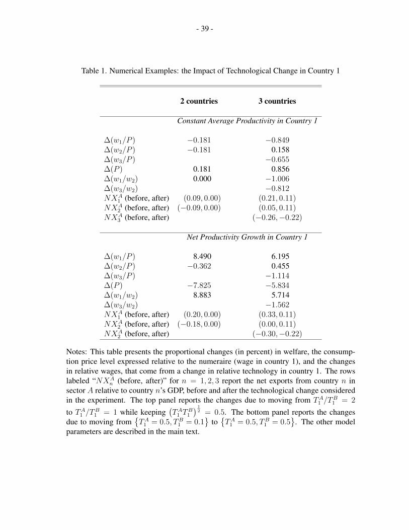
- 39 -
Table 1. Numerical Examples: the Impact of Technological Change in Country 1
2 countries 3 countries
Constant Average Productivity in Country 1
∆(w1/P ) −0.181 −0.849∆(w2/P ) −0.181 0.158∆(w3/P ) −0.655∆(P ) 0.181 0.856∆(w1/w2) 0.000 −1.006∆(w3/w2) −0.812NXA
1 (before, after) (0.09, 0.00) (0.21, 0.11)NXA
2 (before, after) (−0.09, 0.00) (0.05, 0.11)NXA
3 (before, after) (−0.26,−0.22)
Net Productivity Growth in Country 1
∆(w1/P ) 8.490 6.195∆(w2/P ) −0.362 0.455∆(w3/P ) −1.114∆(P ) −7.825 −5.834∆(w1/w2) 8.883 5.714∆(w3/w2) −1.562NXA
1 (before, after) (0.20, 0.00) (0.33, 0.11)NXA
2 (before, after) (−0.18, 0.00) (0.00, 0.11)NXA
2 (before, after) (−0.30,−0.22)
Notes: This table presents the proportional changes (in percent) in welfare, the consump-tion price level expressed relative to the numeraire (wage in country 1), and the changesin relative wages, that come from a change in relative technology in country 1. The rowslabeled “NXA
n (before, after)” for n = 1, 2, 3 report the net exports from country n insector A relative to country n’s GDP, before and after the technological change consideredin the experiment. The top panel reports the changes due to moving from TA1 /T
B1 = 2
to TA1 /TB1 = 1 while keeping
(TA1 T
B1
) 12 = 0.5. The bottom panel reports the changes
due to moving from{TA1 = 0.5, TB1 = 0.1
}to{TA1 = 0.5, TB1 = 0.5
}. The other model
parameters are described in the main text.
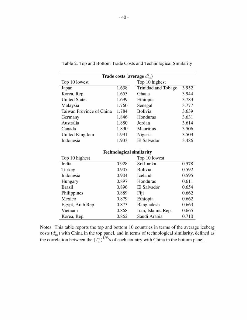
- 40 -
Table 2. Top and Bottom Trade Costs and Technological Similarity
Trade costs (average djni)Top 10 lowest Top 10 highestJapan 1.638 Trinidad and Tobago 3.952Korea, Rep. 1.653 Ghana 3.944United States 1.699 Ethiopia 3.783Malaysia 1.760 Senegal 3.777Taiwan Province of China 1.784 Bolivia 3.639Germany 1.846 Honduras 3.631Australia 1.880 Jordan 3.614Canada 1.890 Mauritius 3.506United Kingdom 1.931 Nigeria 3.503Indonesia 1.933 El Salvador 3.486
Technological similarityTop 10 highest Top 10 lowestIndia 0.928 Sri Lanka 0.578Turkey 0.907 Bolivia 0.592Indonesia 0.904 Iceland 0.595Hungary 0.897 Honduras 0.611Brazil 0.896 El Salvador 0.654Philippines 0.889 Fiji 0.662Mexico 0.879 Ethiopia 0.662Egypt, Arab Rep. 0.873 Bangladesh 0.663Vietnam 0.868 Iran, Islamic Rep. 0.665Korea, Rep. 0.862 Saudi Arabia 0.710
Notes: This table reports the top and bottom 10 countries in terms of the average icebergcosts (djni) with China in the top panel, and in terms of technological similarity, defined asthe correlation between the (T jn)
1/θ’s of each country with China in the bottom panel.
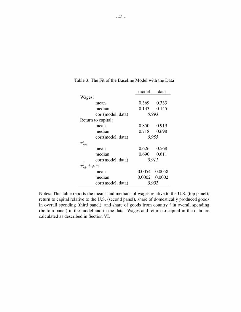
- 41 -
Table 3. The Fit of the Baseline Model with the Data
model dataWages:
mean 0.369 0.333median 0.133 0.145corr(model, data) 0.993
Return to capital:mean 0.850 0.919median 0.718 0.698corr(model, data) 0.955
πjnnmean 0.626 0.568median 0.690 0.611corr(model, data) 0.911
πjni, i 6= nmean 0.0054 0.0058median 0.0002 0.0002corr(model, data) 0.902
Notes: This table reports the means and medians of wages relative to the U.S. (top panel);return to capital relative to the U.S. (second panel), share of domestically produced goodsin overall spending (third panel), and share of goods from country i in overall spending(bottom panel) in the model and in the data. Wages and return to capital in the data arecalculated as described in Section VI.
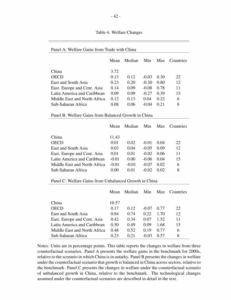
- 42 -
Table 4. Welfare Changes
Panel A: Welfare Gains from Trade with China
Mean Median Min Max Countries
China 3.72OECD 0.13 0.12 -0.03 0.30 22East and South Asia 0.23 0.20 -0.20 0.80 12East. Europe and Cent. Asia 0.14 0.09 -0.08 0.78 11Latin America and Caribbean 0.09 0.09 -0.27 0.39 15Middle East and North Africa 0.12 0.13 0.04 0.22 6Sub-Saharan Africa 0.08 0.06 -0.04 0.21 8
Panel B: Welfare Gains from Balanced Growth in China
Mean Median Min Max Countries
China 11.43OECD 0.01 0.02 -0.01 0.04 22East and South Asia 0.03 0.04 -0.05 0.09 12East. Europe and Cent. Asia 0.01 0.01 -0.02 0.06 11Latin America and Caribbean -0.01 0.00 -0.06 0.04 15Middle East and North Africa -0.01 -0.01 -0.07 0.02 6Sub-Saharan Africa 0.00 0.01 -0.02 0.02 8
Panel C: Welfare Gains from Unbalanced Growth in China
Mean Median Min Max Countries
China 10.57OECD 0.17 0.12 -0.07 0.77 22East and South Asia 0.84 0.74 0.22 1.70 12East. Europe and Cent. Asia 0.42 0.34 0.07 1.52 11Latin America and Caribbean 0.50 0.49 0.09 1.68 15Middle East and North Africa 0.48 0.52 0.19 0.77 6Sub-Saharan Africa 0.23 0.21 -0.03 0.57 8
Notes: Units are in percentage points. This table reports the changes in welfare from threecounterfactual scenarios. Panel A presents the welfare gains in the benchmark for 2000s,relative to the scenario in which China is in autarky. Panel B presents the changes in welfareunder the counterfactual scenario that growth is balanced in China across sectors, relative tothe benchmark. Panel C presents the changes in welfare under the counterfactual scenarioof unbalanced growth in China, relative to the benchmark. The technological changesassumed under the counterfactual scenarios are described in detail in the text.
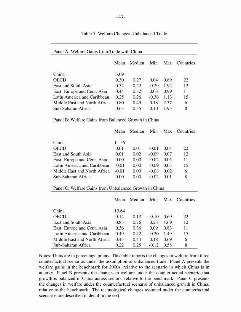
- 43 -
Table 5. Welfare Changes, Unbalanced Trade
Panel A: Welfare Gains from Trade with China
Mean Median Min Max Countries
China 3.09OECD 0.30 0.27 0.04 0.89 22East and South Asia 0.32 0.22 -0.29 1.92 12East. Europe and Cent. Asia 0.44 0.32 0.03 0.99 11Latin America and Caribbean 0.25 0.26 -0.36 1.13 15Middle East and North Africa 0.80 0.49 0.18 2.37 6Sub-Saharan Africa 0.63 0.55 0.10 1.95 8
Panel B: Welfare Gains from Balanced Growth in China
Mean Median Min Max Countries
China 11.56OECD 0.01 0.01 -0.01 0.04 22East and South Asia 0.01 0.02 -0.09 0.07 12East. Europe and Cent. Asia 0.00 0.00 -0.02 0.05 11Latin America and Caribbean -0.01 0.00 -0.09 0.03 15Middle East and North Africa -0.01 0.00 -0.08 0.02 6Sub-Saharan Africa 0.00 0.00 -0.02 0.01 8
Panel C: Welfare Gains from Unbalanced Growth in China
Mean Median Min Max Countries
China 10.64OECD 0.14 0.12 -0.10 0.69 22East and South Asia 0.83 0.76 0.23 1.69 12East. Europe and Cent. Asia 0.36 0.36 0.09 0.83 11Latin America and Caribbean 0.49 0.42 -0.20 1.49 15Middle East and North Africa 0.43 0.44 0.18 0.69 6Sub-Saharan Africa 0.22 0.25 -0.12 0.58 8
Notes: Units are in percentage points. This table reports the changes in welfare from threecounterfactual scenarios under the assumption of unbalanced trade. Panel A presents thewelfare gains in the benchmark for 2000s, relative to the scenario in which China is inautarky. Panel B presents the changes in welfare under the counterfactual scenario thatgrowth is balanced in China across sectors, relative to the benchmark. Panel C presentsthe changes in welfare under the counterfactual scenario of unbalanced growth in China,relative to the benchmark. The technological changes assumed under the counterfactualscenarios are described in detail in the text.
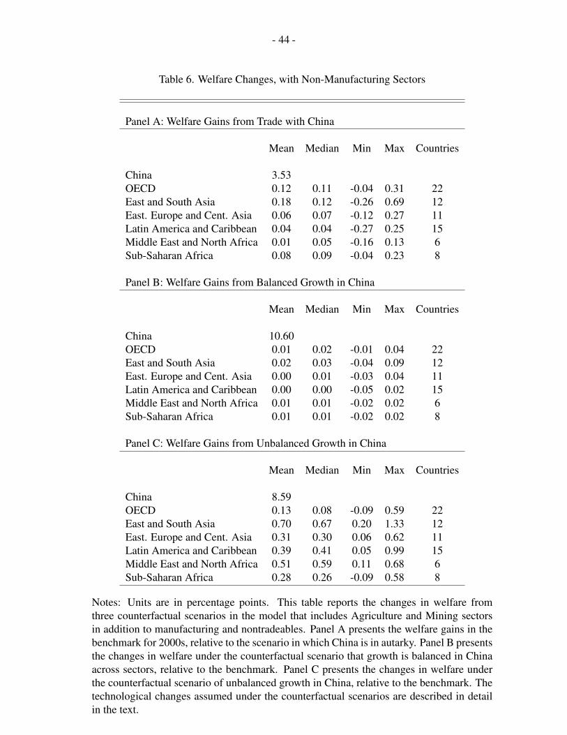
- 44 -
Table 6. Welfare Changes, with Non-Manufacturing Sectors
Panel A: Welfare Gains from Trade with China
Mean Median Min Max Countries
China 3.53OECD 0.12 0.11 -0.04 0.31 22East and South Asia 0.18 0.12 -0.26 0.69 12East. Europe and Cent. Asia 0.06 0.07 -0.12 0.27 11Latin America and Caribbean 0.04 0.04 -0.27 0.25 15Middle East and North Africa 0.01 0.05 -0.16 0.13 6Sub-Saharan Africa 0.08 0.09 -0.04 0.23 8
Panel B: Welfare Gains from Balanced Growth in China
Mean Median Min Max Countries
China 10.60OECD 0.01 0.02 -0.01 0.04 22East and South Asia 0.02 0.03 -0.04 0.09 12East. Europe and Cent. Asia 0.00 0.01 -0.03 0.04 11Latin America and Caribbean 0.00 0.00 -0.05 0.02 15Middle East and North Africa 0.01 0.01 -0.02 0.02 6Sub-Saharan Africa 0.01 0.01 -0.02 0.02 8
Panel C: Welfare Gains from Unbalanced Growth in China
Mean Median Min Max Countries
China 8.59OECD 0.13 0.08 -0.09 0.59 22East and South Asia 0.70 0.67 0.20 1.33 12East. Europe and Cent. Asia 0.31 0.30 0.06 0.62 11Latin America and Caribbean 0.39 0.41 0.05 0.99 15Middle East and North Africa 0.51 0.59 0.11 0.68 6Sub-Saharan Africa 0.28 0.26 -0.09 0.58 8
Notes: Units are in percentage points. This table reports the changes in welfare fromthree counterfactual scenarios in the model that includes Agriculture and Mining sectorsin addition to manufacturing and nontradeables. Panel A presents the welfare gains in thebenchmark for 2000s, relative to the scenario in which China is in autarky. Panel B presentsthe changes in welfare under the counterfactual scenario that growth is balanced in Chinaacross sectors, relative to the benchmark. Panel C presents the changes in welfare underthe counterfactual scenario of unbalanced growth in China, relative to the benchmark. Thetechnological changes assumed under the counterfactual scenarios are described in detailin the text.
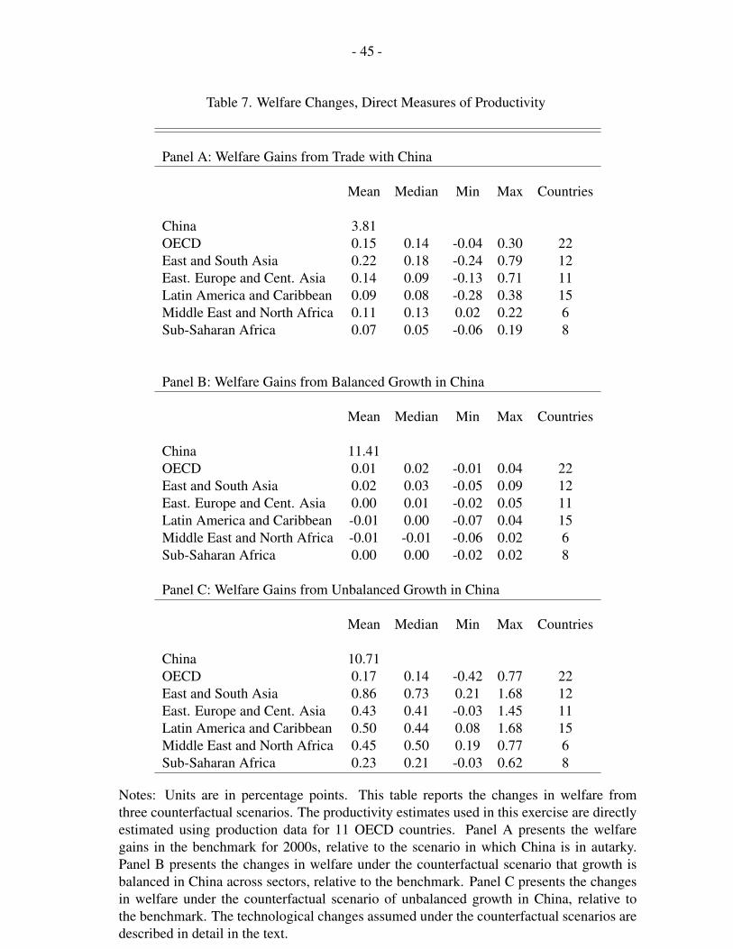
- 45 -
Table 7. Welfare Changes, Direct Measures of Productivity
Panel A: Welfare Gains from Trade with China
Mean Median Min Max Countries
China 3.81OECD 0.15 0.14 -0.04 0.30 22East and South Asia 0.22 0.18 -0.24 0.79 12East. Europe and Cent. Asia 0.14 0.09 -0.13 0.71 11Latin America and Caribbean 0.09 0.08 -0.28 0.38 15Middle East and North Africa 0.11 0.13 0.02 0.22 6Sub-Saharan Africa 0.07 0.05 -0.06 0.19 8
Panel B: Welfare Gains from Balanced Growth in China
Mean Median Min Max Countries
China 11.41OECD 0.01 0.02 -0.01 0.04 22East and South Asia 0.02 0.03 -0.05 0.09 12East. Europe and Cent. Asia 0.00 0.01 -0.02 0.05 11Latin America and Caribbean -0.01 0.00 -0.07 0.04 15Middle East and North Africa -0.01 -0.01 -0.06 0.02 6Sub-Saharan Africa 0.00 0.00 -0.02 0.02 8
Panel C: Welfare Gains from Unbalanced Growth in China
Mean Median Min Max Countries
China 10.71OECD 0.17 0.14 -0.42 0.77 22East and South Asia 0.86 0.73 0.21 1.68 12East. Europe and Cent. Asia 0.43 0.41 -0.03 1.45 11Latin America and Caribbean 0.50 0.44 0.08 1.68 15Middle East and North Africa 0.45 0.50 0.19 0.77 6Sub-Saharan Africa 0.23 0.21 -0.03 0.62 8
Notes: Units are in percentage points. This table reports the changes in welfare fromthree counterfactual scenarios. The productivity estimates used in this exercise are directlyestimated using production data for 11 OECD countries. Panel A presents the welfaregains in the benchmark for 2000s, relative to the scenario in which China is in autarky.Panel B presents the changes in welfare under the counterfactual scenario that growth isbalanced in China across sectors, relative to the benchmark. Panel C presents the changesin welfare under the counterfactual scenario of unbalanced growth in China, relative tothe benchmark. The technological changes assumed under the counterfactual scenarios aredescribed in detail in the text.

- 46 -
Table A1. Country CoverageOECD Latin America and CaribbeanAustralia ArgentinaAustria BoliviaBelgium-Luxembourg BrazilCanada ChileDenmark ColombiaFinland Costa RicaFrance EcuadorGermany El SalvadorGreece GuatemalaIceland HondurasIreland MexicoItaly PeruJapan Trinidad and TobagoNetherlands UruguayNew Zealand Venezuela, RBNorwayPortugal Eastern Europe and Central AsiaSpain BulgariaSweden Czech RepublicSwitzerland HungaryUnited Kingdom KazakhstanUnited States Poland
RomaniaEast and South Asia Russian FederationBangladesh Slovak RepublicChina SloveniaFiji TurkeyIndia UkraineIndonesiaKorea, Rep. Middle East and North AfricaMalaysia Egypt, Arab Rep.Pakistan Iran, Islamic Rep.Philippines IsraelSri Lanka JordanTaiwan Province of China KuwaitThailand Saudi ArabiaVietnam
Sub-Saharan AfricaEthiopiaGhanaKenyaMauritiusNigeriaSenegalSouth AfricaTanzania
Notes: This table reports the countries in the sample.
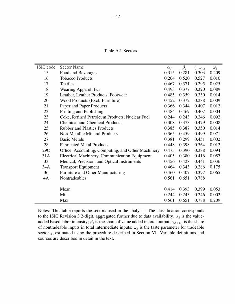
- 47 -
Table A2. Sectors
ISIC code Sector Name αj βj γJ+1,j ωj15 Food and Beverages 0.315 0.281 0.303 0.20916 Tobacco Products 0.264 0.520 0.527 0.01017 Textiles 0.467 0.371 0.295 0.02518 Wearing Apparel, Fur 0.493 0.377 0.320 0.08919 Leather, Leather Products, Footwear 0.485 0.359 0.330 0.01420 Wood Products (Excl. Furniture) 0.452 0.372 0.288 0.00921 Paper and Paper Products 0.366 0.344 0.407 0.01222 Printing and Publishing 0.484 0.469 0.407 0.00423 Coke, Refined Petroleum Products, Nuclear Fuel 0.244 0.243 0.246 0.09224 Chemical and Chemical Products 0.308 0.373 0.479 0.00825 Rubber and Plastics Products 0.385 0.387 0.350 0.01426 Non-Metallic Mineral Products 0.365 0.459 0.499 0.07127 Basic Metals 0.381 0.299 0.451 0.00228 Fabricated Metal Products 0.448 0.398 0.364 0.012
29C Office, Accounting, Computing, and Other Machinery 0.473 0.390 0.388 0.09431A Electrical Machinery, Communication Equipment 0.405 0.380 0.416 0.05733 Medical, Precision, and Optical Instruments 0.456 0.428 0.441 0.036
34A Transport Equipment 0.464 0.343 0.286 0.17536 Furniture and Other Manufacturing 0.460 0.407 0.397 0.0654A Nontradeables 0.561 0.651 0.788
Mean 0.414 0.393 0.399 0.053Min 0.244 0.243 0.246 0.002Max 0.561 0.651 0.788 0.209
Notes: This table reports the sectors used in the analysis. The classification correspondsto the ISIC Revision 3 2-digit, aggregated further due to data availability. αj is the value-added based labor intensity; βj is the share of value added in total output; γJ+1,j is the shareof nontradeable inputs in total intermediate inputs; ωj is the taste parameter for tradeablesector j, estimated using the procedure described in Section VI. Variable definitions andsources are described in detail in the text.

- 48 -
Table A3. Alternative Counterfactuals
Panel A: Summary StatisticsMean St. Dev. Min Max
Balanced 0.01 0.03 -0.07 0.09Unbalanced 0.42 0.39 -0.07 1.70Unbalanced – Linear 0.11 0.12 -0.02 0.56Unbalanced – No Regress 0.28 0.28 -0.06 1.28Unbalanced – U.S. Values 0.43 0.42 -0.10 1.89
Panel B: CorrelationsBalanced Unbalanced Unbalanced Unbalanced
– Linear – No RegressBalanced 1.000Unbalanced 0.065 1.000Unbalanced – Linear -0.157 0.946 1.000Unbalanced – No Regress 0.131 0.984 0.939 1.000Unbalanced – U.S. Values 0.054 0.997 0.937 0.973
Notes: The top panel of this table reports the summary statistics for the different coun-terfactual scenarios for Chinese productivity growth. “Balanced” and “Unbalanced” arethe two main counterfactuals in the paper, depicted graphically in Figure 5. “Unbalanced– Linear” is a counterfactual in which the most productive Chinese sector relative to theworld frontier keeps the same productivity, while each successive sectors’s productivityrelative to the world frontier is lower by a fixed multiplicative constant. “Unbalanced – NoRegress” is a counterfactual in which productivity in each Chinese sector becomes a con-stant ratio to the world frontier, unless that would imply an absolute reduction in sectoralproductivity, in which case the productivity remains unchanged. “Unbalanced – U.S. Val-ues” is a counterfactual in which Chinese productivity relative to the world frontier is thesame as in the U.S. Across all counterfactuals, the geometric average sectoral productivityin Chinese sectors is kept the same. The counterfactuals are depicted graphically in FigureA1.

- 49 -
Figure 1. Chinese Trade, 1962-2007
050
010
0015
00In
dex
1990
=100
1960 1970 1980 1990 2000 2010Year
China World
(a) China and World Trade, Index Number, 1990=100
0.0
5.1
.15
1960 1970 1980 1990 2000 2010Year
OECD
0.0
5.1
.15
1960 1970 1980 1990 2000 2010Year
East and South Asia
0.0
5.1
.15
1960 1970 1980 1990 2000 2010Year
Latin America and Caribbean
0.0
5.1
.15
1960 1970 1980 1990 2000 2010Year
East. Europe and Cent. Asia
0.0
5.1
.15
1960 1970 1980 1990 2000 2010Year
Middle East and North Africa
0.0
5.1
.15
1960 1970 1980 1990 2000 2010Year
Sub−Saharan Africa
Shar
e of
Impo
rts fr
om C
hina
in T
otal
Impo
rts
(b) Share of Imports from China in Total Imports, by Region
Notes: Figure 1(a) plots the total real (inflation-adjusted) exports from China (solid line),and the total real (inflation-adjusted) world exports (dashed line), for the period 1962-2007.Both series are normalized such that the 1990 value equals 100. Figure 1(b) plots the shareof imports coming from China in the total imports of the major world regions, 1962-2007.

- 50 -
Figure 2. Welfare and Technological Similarity: A Numerical Example
0.5 1 1.5 2 2.5
1.125
1.13
1.135
1.14
1.145
Relative Technology in Country 1
Wel
fare
Country 1Country 2
0.5 1 1.5 2 2.51.16
1.17
1.18
1.19
1.2
1.21
Relative Technology in Country 1
Wel
fare
Country 1Country 2
(a) 2-Country Model0.5 1 1.5 2 2.5
1.125
1.13
1.135
1.14
1.145
Relative Technology in Country 1
Wel
fare
Country 1Country 2
0.5 1 1.5 2 2.51.16
1.17
1.18
1.19
1.2
1.21
Relative Technology in Country 1
Wel
fare
Country 1Country 2
(b) 3-Country Model
Notes: This figure plots welfare in country 1 and country 2 as a function of TA1 /TB1 . The
top panel considers a 2-country model, whereas the bottom panel a 3-country model. Forcountry 2, TA2 /T
B2 = 1, so countries 1 and 2 have the same technology when the value on
the x-axis equals 1. Exact parameter values are decribed in Section C.
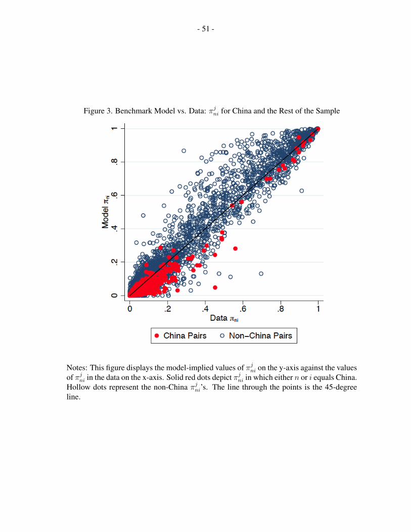
- 51 -
Figure 3. Benchmark Model vs. Data: πjni for China and the Rest of the Sample
Notes: This figure displays the model-implied values of πjni on the y-axis against the valuesof πjni in the data on the x-axis. Solid red dots depict πjni in which either n or i equals China.Hollow dots represent the non-China πjni’s. The line through the points is the 45-degreeline.
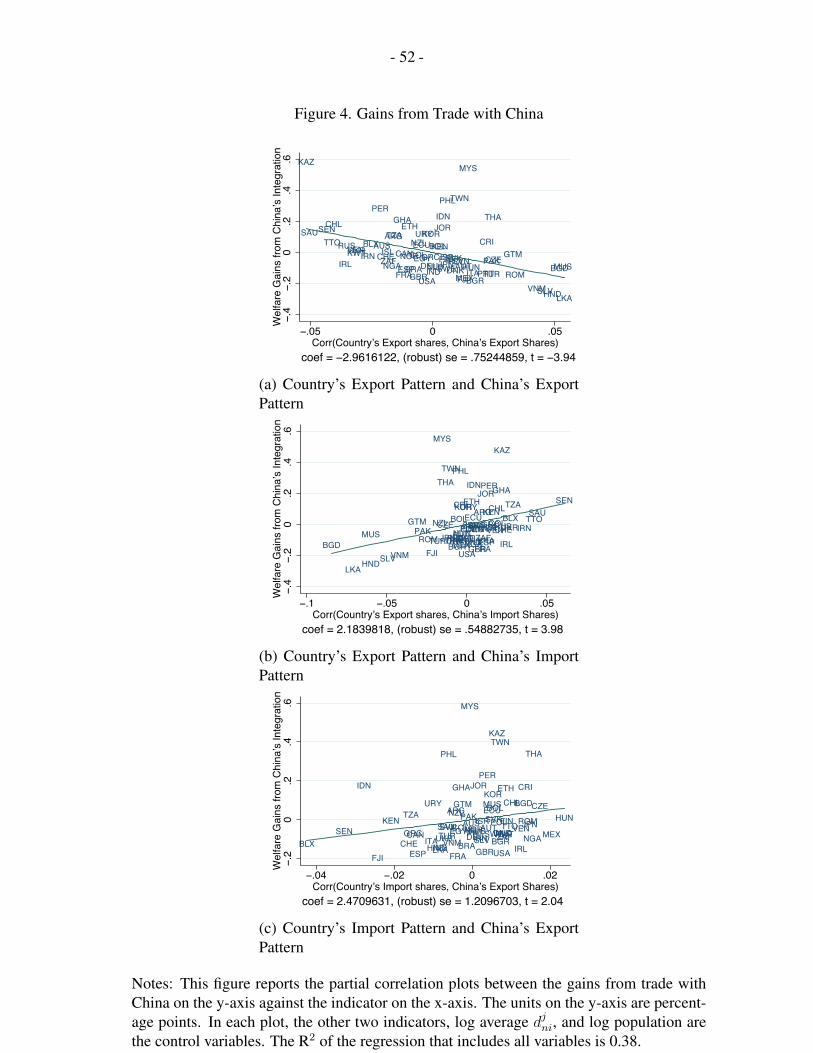
- 52 -
Figure 4. Gains from Trade with China
KAZ
SAUSENTTO
CHL
IRL
RUSVENKWTUKRIRNBLX
PER
AUSCHEISLZAFNGA
ARGTZA
GHA
FRA
CAN
ESPNOR
ETH
BRACOL
GBR
NZLECUEGY
URY
USADEUGRC
KOR
INDNLD
BOLKEN
JORIDN
FINJPNSWEISR
PHL
SVKDNKPOL
TWN
SVN
FJIAUTMEX
MYS
HUNITABGR
PRT
CRI
TURPAK
THA
CZE GTM
ROMVNMSLVHND
BGDMUS
LKA.4
.20
.2.4
.6W
elfa
re G
ains
from
Chi
na’s
Inte
grat
ion
.05 0 .05Corr(Country’s Export shares, China’s Export Shares)
coef = 2.9616122, (robust) se = .75244859, t = 3.94
(a) Country’s Export Pattern and China’s ExportPattern
BGD
LKAHND
MUS
SLVVNM
GTMPAKROM
FJITUR
NZL
MYS
CZE
THA
JPN
TWN
ITADNKPRTBGR
BOL
KWTAUT
PHL
CRI
MEXHUN
KOR
SWENLDDEU
USA
FINPOL
URY
SVK
ETH
ISRECU
NGA
IDN
CANIND
SVNAUS
GBR
EGY
FRA
ARG
ZAF
JOR
BRAESPNOR
PER
GRCISLKEN
VEN
CHLCOL
GHA
KAZ
RUSCHEIRL
UKRBLXTZA
IRNTTOSAU
SEN
.4.2
0.2
.4.6
Wel
fare
Gai
ns fr
om C
hina
’s In
tegr
atio
n
.1 .05 0 .05Corr(Country’s Export shares, China’s Import Shares)
coef = 2.1839818, (robust) se = .54882735, t = 3.98
(b) Country’s Export Pattern and China’s ImportPattern
BLXSEN
IDN
FJI
KEN
CHE
TZA
GRCCAN
ESPITA
URY
HNDINDLKAUKRSAUTURSVN
PHL
VNM
ARGNZL
FRA
EGYCOL
GHA
GTM
BRA
PAK
MYS
AUSISLNORPRTDEURUS
JOR
IRNSLV
ISR
GBR
PER
AUT
ECUMUSKOR
SVKSWE
BOL
KAZ
POL
TWN
BGRUSA
DNKNLDZAFKWT
ETH
FINTTO
CHL
IRL
VEN
BGD
CRI
ROMJPNNGA
THA
CZE
MEX
HUN
.20
.2.4
.6W
elfa
re G
ains
from
Chi
na’s
Inte
grat
ion
.04 .02 0 .02Corr(Country’s Import shares, China’s Export Shares)
coef = 2.4709631, (robust) se = 1.2096703, t = 2.04
(c) Country’s Import Pattern and China’s ExportPattern
Notes: This figure reports the partial correlation plots between the gains from trade withChina on the y-axis against the indicator on the x-axis. The units on the y-axis are percent-age points. In each plot, the other two indicators, log average djni, and log population arethe control variables. The R2 of the regression that includes all variables is 0.38.
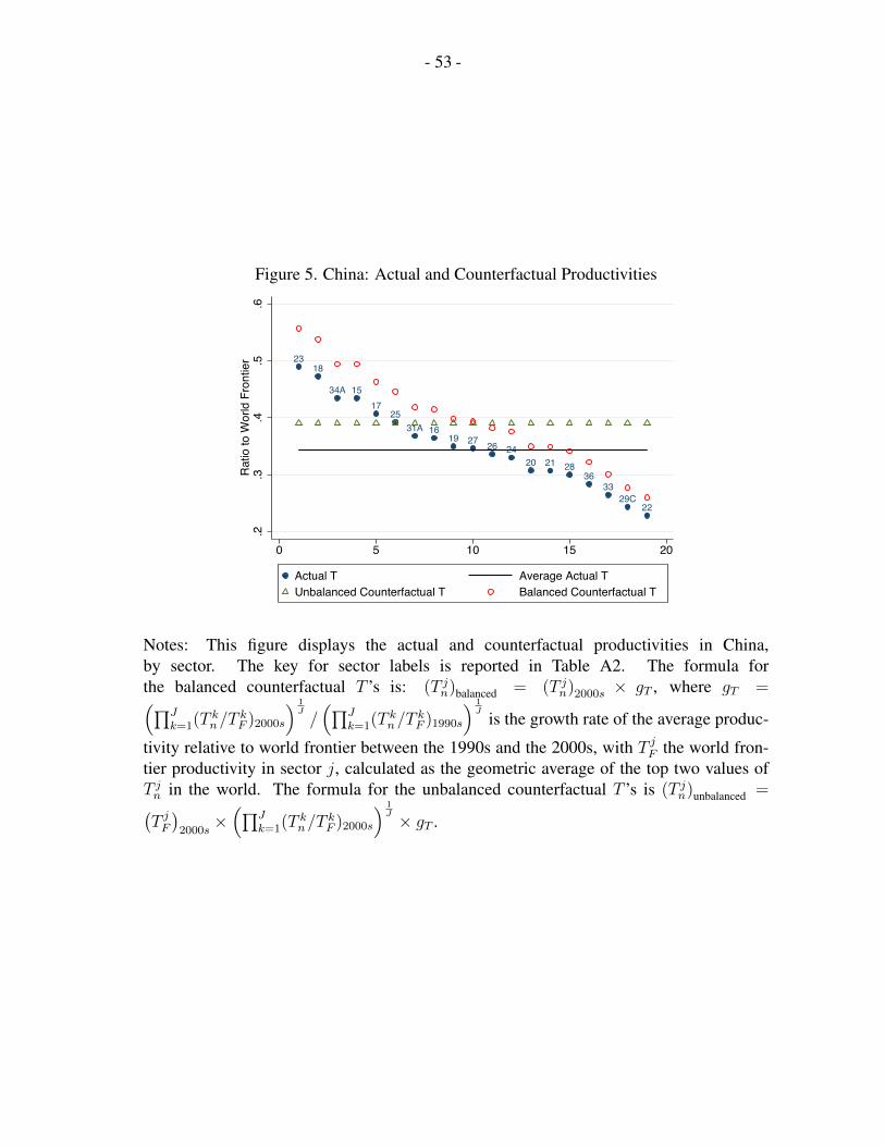
- 53 -
Figure 5. China: Actual and Counterfactual Productivities
15
16
17
18
19
20 21
22
23
24
25
2627
28
29C
31A
33
34A
36
.2.3
.4.5
.6Ra
tio to
Wor
ld F
ront
ier
0 5 10 15 20
Actual T Average Actual TUnbalanced Counterfactual T Balanced Counterfactual T
Notes: This figure displays the actual and counterfactual productivities in China,by sector. The key for sector labels is reported in Table A2. The formula forthe balanced counterfactual T ’s is: (T jn)balanced = (T jn)2000s × gT , where gT =(∏J
k=1(Tkn/T
kF )2000s
) 1J/(∏J
k=1(Tkn/T
kF )1990s
) 1J
is the growth rate of the average produc-
tivity relative to world frontier between the 1990s and the 2000s, with T jF the world fron-tier productivity in sector j, calculated as the geometric average of the top two values ofT jn in the world. The formula for the unbalanced counterfactual T ’s is (T jn)unbalanced =(T jF)2000s
×(∏J
k=1(Tkn/T
kF )2000s
) 1J × gT .
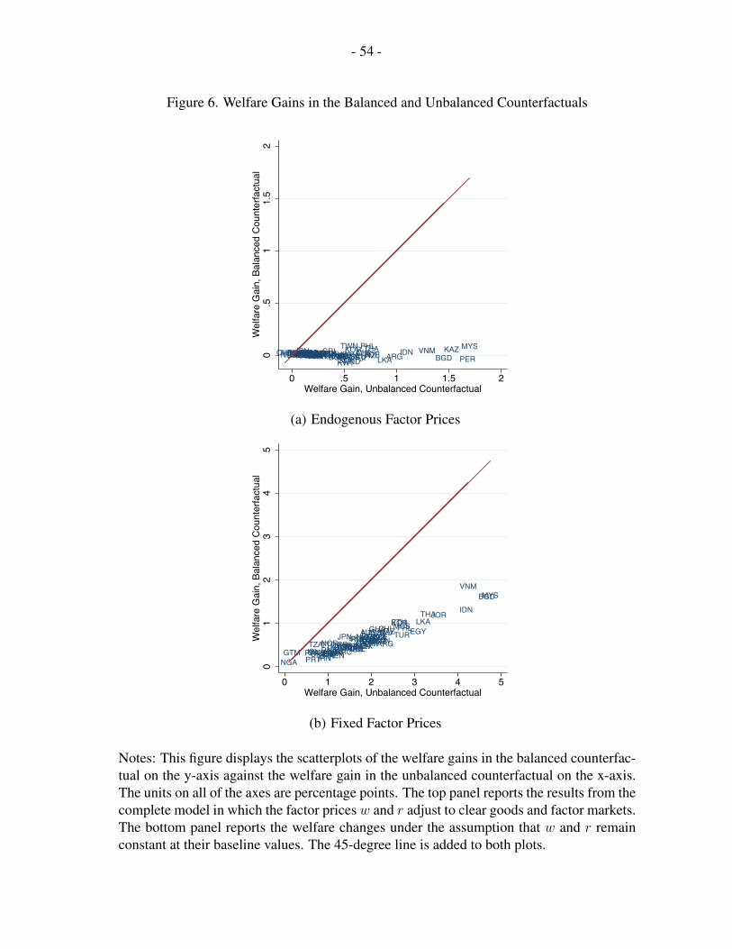
- 54 -
Figure 6. Welfare Gains in the Balanced and Unbalanced Counterfactuals
LKABOLISLHNDSLV FJIETH BGDIRN SAUROMISRSVKIRL RUSSWENOR THAMUSNLDFINBLX ECUSVNCHE UKR
MYSITA KAZ
PERTZAKWT
CZE NZLURY JORCHLGTMSENDNKGRCESP VENPRT ZAFNGATWN
GBRUSATTO AUSBGRPAKGHACANDEUFRAAUTJPNPOL CRIKENCOL ARGKOR VNMEGYMEX
PHLBRA HUN IDNTURIND0
.51
1.5
2W
elfa
re G
ain,
Bal
ance
d C
ount
erfa
ctua
l
0 .5 1 1.5 2Welfare Gain, Unbalanced Counterfactual
(a) Endogenous Factor Prices
LKA
BOL
ISLHNDSLV
FJIETH
BGD
IRN
SAUROMISR
SVKIRLRUS
SWENOR
THAMUS
NLDFINBLX
ECUSVNCHE
UKR
MYS
ITA
KAZPERTZA KWT
CZENZLURY
JOR
CHL
GTMSENDNKGRCESP VEN
PRT
ZAF
NGA
TWN
GBRUSATTOAUS
BGRPAK
GHACAN
DEUFRAAUT
JPN POLCRIKEN
COL ARG
KOR
VNM
EGY
MEX
PHL
BRA
HUN
IDN
TURIND
01
23
45
Wel
fare
Gai
n, B
alan
ced
Cou
nter
fact
ual
0 1 2 3 4 5Welfare Gain, Unbalanced Counterfactual
(b) Fixed Factor Prices
Notes: This figure displays the scatterplots of the welfare gains in the balanced counterfac-tual on the y-axis against the welfare gain in the unbalanced counterfactual on the x-axis.The units on all of the axes are percentage points. The top panel reports the results from thecomplete model in which the factor prices w and r adjust to clear goods and factor markets.The bottom panel reports the welfare changes under the assumption that w and r remainconstant at their baseline values. The 45-degree line is added to both plots.

- 55 -
Figure 7. China’s and World Average Comparative Advantage
15
17
18
19
2021
22
23
24
25
2627
28
29C
31A
33
34A
36
.2.3
.4.5
Chi
na’s
Dis
tanc
e to
Fro
ntie
r
.45 .5 .55 .6 .65 .7Global Average Distance to Frontier
Notes: This figure displays the distance to the global frontier in each sector in China (y-axis) against the simple average of the distance to frontier in that sector in the world ex-cluding China. The key for sector labels is reported in Table A2.
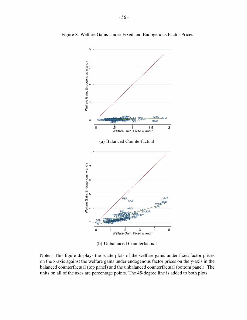
- 56 -
Figure 8. Welfare Gains Under Fixed and Endogenous Factor Prices
LKABOLISLHNDSLV FJI ETH BGDIRN SAUROMISR SVKIRL RUSSWE NOR THA
MUSNLDFINBLX ECUSVNCHE UKRMYS
ITA KAZPERTZA
KWTCZENZLURY JORCHLGTMSENDNKGRCESPVENPRT ZAFNGA
TWNGBRUSATTO AUSBGRPAK GHACANDEUFRAAUT JPNPOLCRIKENCOLARG
KOR VNMEGYMEXPHL
BRA HUN IDNTURIND0.5
11.
52
Wel
fare
Gai
n, E
ndog
enou
s w
and
r
0 .5 1 1.5 2Welfare Gain, Fixed w and r
(a) Balanced Counterfactual
LKA
BOL
ISL
HNDSLVFJI
ETH
BGD
IRN
SAUROM
ISR SVKIRLRUS
SWENOR
THAMUS
NLDFINBLXECU
SVNCHE
UKR
MYS
ITA
KAZPER
TZA
KWTCZE
NZLURY
JORCHL
GTM SENDNKGRCESP
VEN
PRTZAF
NGA
TWN
GBRUSATTO
AUSBGR
PAK GHACAN
DEUFRAAUTJPN POLCRI
KEN COL
ARG
KOR
VNM
EGYMEX
PHL
BRAHUN
IDN
TURIND
01
23
45
Wel
fare
Gai
n, E
ndog
enou
s w
and
r
0 1 2 3 4 5Welfare Gain, Fixed w and r
(b) Unbalanced Counterfactual
Notes: This figure displays the scatterplots of the welfare gains under fixed factor priceson the x-axis against the welfare gains under endogenous factor prices on the y-axis in thebalanced counterfactual (top panel) and the unbalanced counterfactual (bottom panel). Theunits on all of the axes are percentage points. The 45-degree line is added to both plots.

- 57 -
Figure 9. Unbalanced Counterfactual Welfare Gains and Technological Similarity
LKA
BOL
ISL
HNDSLV
FJI
ETH
BGD
IRN
SAU
ROM
ISRSVK
IRL
RUS
SWENOR
THA
MUS
NLDFINBLX
ECU
SVN
CHE
UKR
MYS
ITA
KAZ
PER
TZA
KWT
CZE
NZL
URY
JORCHL
GTMSENDNK
GRCESP
VEN
PRT
ZAF
NGA
TWN
GBRUSA
TTO
AUS
BGR
PAKGHACAN
DEUFRAAUTJPN
POL
CRI
KENCOL
ARG
KOR
VNM
EGY
MEX
PHL
BRA
HUN
IDN
TUR
IND
0.5
11.
52
Wel
fare
Gai
n, U
nbal
ance
d Co
unte
rfact
ual
.2 .1 0 .1 .2 .3Change in the Correlation of T’s with China
(a) Endogenous Factor Prices
LKA
BOL
ISL
HNDSLV FJI
ETH
BGD
IRN
SAU
ROM
ISR
SVK
IRLRUS
SWENOR
THA
MUS
NLD
FINBLX
ECU
SVN
CHE
UKR
MYS
ITA
KAZ
PER
TZA
KWT
CZE
NZLURY
JOR
CHL
GTM
SEN
DNK
GRCESP
VEN
PRT
ZAF
NGA
TWN
GBRUSA
TTO
AUSBGR
PAK
GHA CAN
DEU
FRAAUT
JPN
POL
CRIKEN
COL
ARG
KOR
VNM
EGY
MEX
PHL
BRA
HUN
IDN
TUR
IND
01
23
45
Wel
fare
Gai
n, U
nbal
ance
d Co
unte
rfact
ual
.2 .1 0 .1 .2 .3Change in the Correlation of T’s with China
(b) Fixed Factor Prices
Notes: This figure displays the scatterplots of the welfare gains in the unbalanced coun-terfactual on the y-axis against the change in the technological between the country andChina. The units on the y-axis are percentage points. Technological similarity is measuredas the correlation coefficient of the T’s between the country and China. On the y-axis isthe simple change in that correlation coefficient. The top panel reports the results from thecomplete model in which the factor prices w and r adjust to clear goods and factor markets.The bottom panel reports the welfare changes under the assumption that w and r remainconstant at their baseline values. The OLS best fit line is added to both plots.
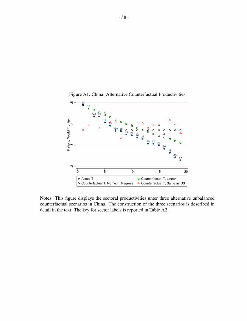
- 58 -
Figure A1. China: Alternative Counterfactual Productivities
2318
34A 15
1725
31A 1619 27
26 24
20 21 2836
3329C
22
.2.3
.4.5
Ratio
to W
orld
Fro
ntie
r
0 5 10 15 20
Actual T Counterfactual T, LinearCounterfactual T, No Tech. Regress Counterfactual T, Same as US
Notes: This figure displays the sectoral productivities unter three alternative unbalancedcounterfactual scenarios in China. The construction of the three scenarios is described indetail in the text. The key for sector labels is reported in Table A2.

- 59 -
REFERENCES
Autor, David, David Dorn, and Gordon Hanson, 2011, “The China Syndrome: Local LaborMarket Effects of Import Competition in the United States,” August, mimeo (MIT,CEMFI, and UC San Diego).
Bartelsman, Eric J. and Wayne Gray, 1996, “The NBER Manufacturing ProductivityDatabase,” October, NBER Technical Working Paper 205.
Bernanke, Ben and Refet Gurkaynak, 2001, “Is Growth Exogenous? Taking Mankiw, Romer,and Weil Seriously,” NBER Macroeconomics Annual, Vol. 16, pp. 11–57.
Berthelon, Matias and Caroline Freund, 2008, “On the Conservation of Distance inInternational Trade,” Journal of International Economics, Vol. 75, No. 2 , July,pp. 310–320.
Bloom, Nicholas, Mirko Draca, and John Van Reenen, 2011, “Trade Induced TechnicalChange: The Impact of Chinese Imports on Innovation, Diffusion and Productivity,”January, NBER Working Paper No. 16717.
Burstein, Ariel and Jonathan Vogel, 2009, “Globalization, Technology, and the SkillPremium,” October, mimeo (UCLA and Columbia University).
Caliendo, Lorenzo and Fernando Parro, 2010, “Estimates of the Trade and Welfare Effects ofNAFTA,” January, mimeo (University of Chicago).
Caselli, Francesco, “Accounting for Cross-Country Income Differences,” 2005, inSteven Durlauf Philippe Aghion, ed., Handbook of Economic Growth, Vol. 1,Elsevier-North Holland, Chapter 9, pp. 679–741.
Chaney, Thomas, 2008, “Distorted Gravity: The Intensive and Extensive Margins ofInternational Trade,” American Economic Review, Vol. 98, No. 4, September,pp. 1707–1721.
Costinot, Arnaud, Dave Donaldson, and Ivana Komunjer, 2011, “What Goods Do CountriesTrade? A Quantitative Exploration of Ricardo’s Ideas,” April, forthcoming, Review ofEconomic Studies.
Dekle, Robert, Jonathan Eaton, and Samuel Kortum, 2007, “Unbalanced Trade,” AmericanEconomic Review: Papers and Proceedings, Vol. 97, No. 2, May, pp. 351–355.
———, ———, and ———, 2008, “Global Rebalancing with Gravity: Measuring theBurden of Adjustment,” IMF Staff Papers, Vol. 55, No. 3, pp. 511–540.
Devlin, Robert, Antoni Estevaeordal, and Andres Rodrıguez-Clare, eds, 2005, The Emergenceof China: Opportunities and Challenges for Latin America and the Caribbean(Cambridge, Mass.: Harvard University Press).
- 60 -
di Giovanni, Julian and Andrei A. Levchenko, 2010, “Putting the Parts Together: Trade,Vertical Linkages, and Business Cycle Comovement,” American Economic Journal:Macroeconomics, Vol. 2, No. 2, April, pp. 95–124.
Do, Quy-Toan and Andrei A. Levchenko, 2007, “Comparative Advantage, Demand forExternal Finance, and Financial Development,” Journal of Financial Economics, Vol.86, No. 3, December, pp. 796–834.
Dornbusch, Rudiger, Stanley Fischer, and Paul Samuelson, 1977, “Comparative Advantage,Trade, and Payments in a Ricardian Model with a Continuum of Goods,” AmericanEconomic Review, Vol. 67, pp. 823–39.
Eaton, Jonathan and Samuel Kortum, 2002, “Technology, Geography, and Trade,”Econometrica, Vol. 70, No. 5, September, pp. 1741–1779.
———, ———, Brent Neiman, and John Romalis, 2010, “Trade and the Global Recession,”July, mimeo (Penn State University and University of Chicago).
Finicelli, Andrea, Patrizio Pagano, and Massimo Sbracia, 2009a, “Ricardian Selection,”October, (Bank of Italy Temi di Discussione), Working Paper No. 728.
Francois, Joseph F. and Ganeshan Wignaraja, 2008, “Economic Implications of AsianIntegration,” Global Economy Journal, Vol. 8, No. 3.
Gallagher, Kevin P., Juan Carlos Moreno-Brid, and Roberto Porzecanski, 2008, “TheDynamism of Mexican Exports: Lost in (Chinese) Translation?,” World Development,Vol. 36, No. 8, pp. 1365–1380.
Ghosh, Madanmohan and Someshwar Rao, 2010, “Chinese Accession to the WTO: EconomicImplications for China, Other Asian and North American Economies,” Journal of PolicyModeling, Vol. 32, No. 3, May–June, pp. 389–98.
Hall, Robert and Charles Jones, 1999, “Why Do Some Countries Produce So Much MoreOutput per Worker then Others,” Quarterly Journal of Economics, Vol. 114, pp. 83–116.
Helpman, Elhanan, Marc J. Melitz, and Stephen R. Yeaple, 2004, “Export versus FDI withHeterogeneous Firms,” American Economic Review, Vol. 94, No. 1, March, pp. 300–316.
Hicks, John, 1953, “An Inaugural Lecture,” Oxford Economic Papers, Vol. 5, No. 2, June,pp. 117–135.
Hsieh, Chang-Tai and Ralph Ossa, 2011, “A Global View of Productivity Growth in China,”(February). NBER Working Paper No. 16778.
Hummels, David, Jun Ishii, and Kei-Mu Yi, 2001, “The Nature and Growth of VerticalSpecialization in World Trade,” Journal of International Economics, Vol. 54, June,pp. 75–96.
- 61 -
Ju, Jiandong and Xuebing Yang, 2009, “Hicks theorem: Effects of technological improvementin the Ricardian model,” International Review of Economics and Finance, Vol. 18,pp. 239–247.
Levchenko, Andrei A. and Jing Zhang, 2011, “The Evolution of Comparative Advantage:Measurement and Welfare Implications,” February, NBER Working Paper No. 16806.
Samuelson, Paul A., 2004, “Where Ricardo and Mill Rebut and Confirm Arguments ofMainstream Economists Supporting Globalization,” Journal of Economic Perspectives,Vol. 18, No. 3, pp. 135–146.
Shikher, Serge, 2004, “Putting industries into the Eaton-Kortum model,” July, forthcoming,Journal of International Trade and Economic Development.
———, 2005, “Accounting for International Trade,” August, mimeo (Suffolk University).
———, 2011, “Capital, technology, and specialization in the neoclassical model,” Journal ofInternational Economics, Vol. 83, No. 2, March, pp. 229–242.
Simonovska, Ina and Michael E. Waugh, 2010, “The Elasticity of Trade: Estimates andEvidence,” December, mimeo (UC Davis and NYU).
Tokarick, Stephen, 2011, “The Implications of China’s Pattern of Growth For the Rest of theWorld,” August, mimeo (International Monetary Fund).
Waugh, Michael, 2010, “International Trade and Income Differences,” American EconomicReview, Vol. 100, No. 5 (December), pp. 2093–2124.
Yi, Kei-Mu and Jing Zhang, 2010, “Structural Change in an Open Economy,” April, mimeo(Federal Reserve Bank of Philadelphia and University of Michigan).


