Sarah L. Martell,17,16 Thomas Nordlander,10,16 Andrew B. Pace,19 Gayandhi M. De Silva,14,16 and Mei-Yu Wang1
(S5 collaboration)1 McWilliams Center for Cosmology, Carnegie Mellon University, 5000 Forbes Ave, Pittsburgh, PA 15213, USA2 Institute of Astronomy, University of Cambridge, Madingley Road, Cambridge CB3 0HA, UK3 Magdalen College, University of Oxford, High Street, Oxford OX1 4AU, UK4 Observatories of the Carnegie Institution for Science, 813 Santa Barbara St., Pasadena, CA 91101, USA5 Department of Astrophysical Sciences, Princeton University, Princeton, NJ 08544, USA6 Hubble Fellow7 Fermi National Accelerator Laboratory, P.O. Box 500, Batavia, IL 60510, USA8 Kavli Institute for Cosmological Physics, University of Chicago, Chicago, IL 60637, USA9 Department of Physics, University of Surrey, Guildford GU2 7XH, UK10 Research School of Astronomy and Astrophysics, Australian National University, Canberra, ACT 2611, Australia11 Department of Physics & Astronomy, Macquarie University, Sydney, NSW 2109, Australia12 Macquarie University Research Centre for Astronomy, Astrophysics & Astrophotonics, Sydney, NSW 2109, Australia13 Lowell Observatory, 1400 W Mars Hill Rd, Flagstaff, AZ 86001, USA14 Australian Astronomical Optics, Faculty of Science and Engineering, Macquarie University, Macquarie Park, NSW 2113, Australia15 Sydney Institute for Astronomy, School of Physics, A28, The University of Sydney, NSW 2006, Australia16 Centre of Excellence for All-Sky Astrophysics in Three Dimensions (ASTRO 3D), Australia17 School of Physics, UNSW, Sydney, NSW 2052, Australia18 Department of Astronomy & Astrophysics, University of Chicago, 5640 S Ellis Avenue, Chicago, IL 60637, USA19 George P. and Cynthia Woods Mitchell Institute for Fundamental Physics and Astronomy, and Department of Physics and Astronomy, Texas A&MUniversity,College Station, TX 77843, USA
Accepted XXX. Received YYY; in original form ZZZ
ABSTRACTWe present the serendipitous discovery of the fastest Main Sequence hyper-velocity star (HVS)by the Southern Stellar Stream Spectroscopic Survey (S5). The star S5-HVS1 is a ∼ 2.35M�A-type star located at a distance of ∼ 9 kpc from the Sun and has a heliocentric radial velocityof 1017 ± 2.7 km s−1 without any signature of velocity variability. The current 3-D velocityof the star in the Galactic frame is 1755 ± 50 km s−1. When integrated backwards in time,the orbit of the star points unambiguously to the Galactic Centre, implying that S5-HVS1was kicked away from Sgr A* with a velocity of ∼ 1800 km s−1 and travelled for 4.8Myrto its current location. This is so far the only HVS confidently associated with the GalacticCentre. S5-HVS1 is also the first hyper-velocity star to provide constraints on the geometryand kinematics of the Galaxy, such as the Solar motion Vy,� = 246.1± 5.3 km s−1 or positionR0 = 8.12 ± 0.23 kpc. The ejection trajectory and transit time of S5-HVS1 coincide with theorbital plane and age of the annular disk of young stars at the Galactic centre, and thus may belinked to its formation. With the S5-HVS1 ejection velocity being almost twice the velocity ofother hyper-velocity stars previously associated with the Galactic Centre, we question whetherthey have been generated by the same mechanism or whether the ejection velocity distributionhas been constant over time.Key words: stars: kinematics and dynamics – Galaxy: centre – Galaxy: fundamental param-eters
Throughout the last 100 years of studying our Galaxy, there wasalways a prominent niche in identifying fast moving stars on the skyor in 3-D. One of the first studies of high-velocity stars was the PhDthesis by Oort (1926) who put a boundary between high velocityand low velocity stars at 63 km s−1. Initially, the searches for fastmoving stars were focused on using the propermotions (vanMaanen1917; Luyten 1979) because these were easier to obtain in largernumbers than radial velocities. Due to the fact that the tangentialvelocities are distance dependent, these searches provided us withsome of the first large samples of nearby andMilkyWay (MW) halostars (Barnard 1916; Eggen & Greenstein 1967; Eggen 1983).
When larger numbers of radial velocities began to be analysedin the 1950s–1960s (Kennedy & Przybylski 1963) the term "highvelocity star" was used to refer to the stars with space velocities of&100 km s−1 (Keenan & Keller 1953), where those stars were mostlyMW stellar halo stars (Eggen et al. 1962). Around the same time,another type of high velocity object emerged – the runawayOB stars(Blaauw & Morgan 1954). These stars did not have extreme spacevelocities, but instead were just offset from the expected velocity ofthe disk by 100-200 km s−1. Some stars were later found in the MWhalo (Greenstein & Sargent 1974) with velocities up to 200 km s−1.The mechanism proposed for the formation of such high velocitystars involves either a supernovae explosion in a binary (Blaauw1961) or ejection due to encounters in clusters (Poveda et al. 1967).
For a while these pathways seemed to be the most promisingfor creating fast moving stars in the Galaxy with velocities poten-tially up to the escape speed. However Hills (1988) proposed anentirely new mechanism of creating fast moving stars with veloci-ties of 1000 km s−1 and above (labelled hyper-velocity stars, HVS)by interaction of a stellar binary with a super-massive Black Hole(SMBH) in the centres of galaxies. This mechanism was almost for-gotten until the early 2000s, when Yu & Tremaine (2003) analysedthe ejection mechanism from single and binary SMBHs and Brownet al. (2005) identified a star in the Milky Way halo at a distance of40 − 70 kpc with a total velocity of ∼ 700 km s−1, well above theescape velocity at such a distance. This discovery spurred a renewedinterest in hyper-velocity stars (Edelmann et al. 2005; Hirsch et al.2005; Heber et al. 2008; Przybilla et al. 2008) and led to dedicatedsearches, resulting in multiple new HVS (Zheng et al. 2014; Huanget al. 2017; Irrgang et al. 2019) and candidate HVS (see Brown2015, for a detailed overview and more references).
The most recent part of the story is the arrival of Gaia data(Gaia Collaboration et al. 2016), in particular Data Release 2 (GaiaCollaboration et al. 2018) that provided high accuracy proper mo-tions, and thus enabled new discoveries (Shen et al. 2018), potentialdiscoveries (Marchetti et al. 2018; Hattori et al. 2018a; Bromleyet al. 2018; Boubert et al. 2019) as well as detailed studies of theHVS origins (Boubert et al. 2018; Brown et al. 2018; Irrgang et al.2018; Erkal et al. 2019). One of the key conclusions from thesestudies is that despite the large number of HVS candidates, only ahandful of these appear to be actually unbound from the Galaxy andconsistent with ejection from the Galactic Centre (GC).
Whilst the extreme speed of several of the HVS in the outerhalo is seemingly unexplainable without the Hills mechanism, theuncertainties on their distances and propermotions are such that theycannot be tracked back precisely to the GC. The most convincingassociation to date is the star J01020100-7122208, identified byMassey et al. (2018) as a bound runaway star that in a particularchoice of potential tracked back to the Galactic Centre; however, thelow 3-D velocity of 296 km s−1 does not preclude a more standard
origin. There is not yet an example of an HVS that unequivocallytracks back to the GC, and thus no smoking gun for a GC Hillsmechanism ejection. The power of HVS as probes of the Galacticpotential (Gnedin et al. 2005) and the orbit of the Sun (Hattori et al.2018b) is contingent on an unambiguous GC origin, and thus it isof paramount importance that such a smoking gun is found.
In this paper we present the discovery of a new nearby unboundHVS that can be unambiguously traced back to the Galactic Centre.The star is named S5-HVS1 as it was found in the Southern StellarStream Spectroscopic Survey (S5, Li et al. 2019).
The structure of the paper is as follows. In Section 2 we brieflyintroduce the S5 survey data that was used to identify the S5-HVS1star and the search for HVS stars in S5 data. In Section 3 we lookat the spectroscopic and photometric properties of S5-HVS1. InSection 4 we analyse the kinematics of the star and its possibleorigin in the Galaxy. In Section 5 we focus on the Galactic Centreas a source of S5-HVS1 as well as inferences we can make on theGalactic potential, distance and velocity of the Sun with respect totheGalactic Centre.We discuss S5-HVS1 inmore detail in Section 6by comparing it to other HVS, as well as examining HVS ejectionmechanisms. Our conclusions are given in Section 7.
2 DATA
The S5 project is a survey devoted to the observation of stellarstreams in the Southern Hemisphere (Li et al. 2019). The sur-vey is being conducted on the 3.9m Anglo-Australian Telescope(AAT) with the Two-degree Field (2dF) fibre positioner feeding theAAOmega dual arm spectrograph (Lewis et al. 2002; Sharp et al.2006). S5 uses low (580V, R ∼ 1300) and high (1700D, R ∼ 10000)resolution gratings in the blue and red wavelength ranges respec-tively, covering the Balmer break region (3800 < λ < 5800Å) inthe blue and IR Calcium triplet (8400 < λ < 8800Å) in the red.The survey is ongoing, but by early 2019 it had observed 110 fieldsspread across ∼330 square degrees and ∼40000 targets. For detailswe refer the reader to the Li et al. (2019) paper, while providinghere only the key aspects of the survey.
S5 is primarily targeting stellar stream candidate members, se-lected based on photometric information from the Dark Energy Sur-vey (DES) DR1 (Abbott et al. 2018) and proper motion and parallaxinformation fromGaiaDR2 (Gaia Collaboration et al. 2016, 2018).To fill all the 392 fibres of the spectrograph other target classes areobserved, including low-redshift galaxy candidates, white dwarfs(WDs), and metal-poor stars, etc. The survey specifically targetsblue stars that could be either Blue Horizontal Branch (BHB) stars,Blue Stragglers (BS) or RR Lyrae stars at a large range of distances.The selection used by S5 for the BHB/BS stars is −0.4 < (g − r) <0.1 and parallax < 3∗parallax_error+0.2, combinedwith thestar-galaxy separation criteria usingastrometric_excess_noisequantities from Gaia (Lindegren et al. 2018; Koposov et al. 2017)and wavg_spread_model quantities from DES (see Eq. 1-3 in Liet al. 2019). At the time of writing the S5 catalogue contains spec-tra of ∼ 3500 blue faint objects. While many of them end up beingquasars (see Li et al. 2019),& 2200 of them are likely BHB/BS/WDstars.
The data processing of the S5 data includes standard data re-duction steps by the AAT pipeline, followed by spectral modelling
MNRAS 000, 1–16 (2019)
S5-HVS1 3
by the rvspecfit1 software in order to determine the radial velocitiesand stellar atmospheric parameters.
2.1 HVS star search
While identifying hyper-velocity stars was not a main goal of theS5 survey, the catalogue of radial velocities (RVs) and spectral fitswas inspected for stars with velocities larger than 800 km s−1. Themajority of objects with such highRVswere spuriousmeasurementscaused by either sky subtraction residuals and/or low signal-to-noisespectra, however the search identified a single bright (G ∼ 16)star with the Gaia DR2 source_id 6513109241989477504 and(α, δ) = (343.715345◦,−51.195607◦), located in the field of theJhelum stellar stream, a new stellar stream found in the DES (Shippet al. 2018). This star had a confident radial velocity measurementof ∼ 1020 km s−1, making it one of the fastest moving stars knownin the Galaxy. The radial velocity of this star alone, irrespectiveof the distance, is enough to make the star unbound to the Galaxy(see e.g. Kafle et al. 2014). We label this star S5-HVS12. In thenext sections we focus on the detailed measurements of S5-HVS1properties: spectroscopic, photometric and kinematic.
3 S5-HVS1 PROPERTIES
In this section we discuss the key spectroscopic properties of S5-HVS1 as determined from AAT data, as well as all available pho-tometric data. The summary of these measurements is presented inTable 1.
3.1 Spectroscopy
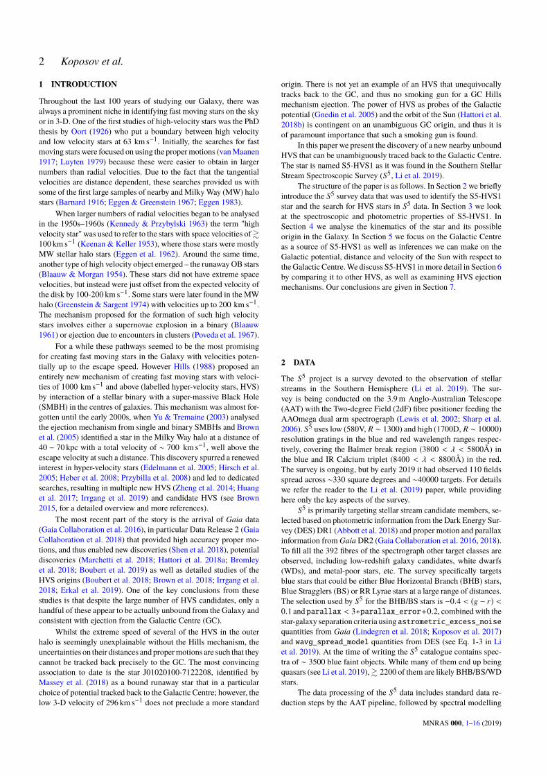
The star S5-HVS1 was observed for the first time at the AAT aspart of regular S5 observations of the Jhelum stellar stream with the580V and 1700Dgratings on 2018August 1. The total exposure timewas 2 hours split into three individual exposures. The combined,reduced spectra for S5-HVS1 are shown in Figure 1. Based on thespectra, the star appears to be a hot A-type star with prominentbroad Balmer and Paschen series and several metal lines like Ca IIH/K and Mg II (4481Å) in the blue and Calcium triplet in the red.
Although the stellar spectra of S5-HVS1 in both the blue andred arms were analysed as part of the regular S5 processing (see Liet al. 2019), the analysis treated the blue and red arms separately.For this paper, however, we analyse the blue and red parts of spec-tra simultaneously in order to better constrain stellar atmosphericparameters. The fitting of stellar spectra is analogous to the proce-dure described in the S5 overview paper and uses the rvspecfit,but instead of considering the likelihood function of the red arm orblue arm data separately, we combine them. Specifically the modelfor the stellar spectrum uses a combination of global Radial BasisFunction interpolation and local linear N-d interpolation of spectrafrom the PHOENIX-2.0 library (Husser et al. 2013) together witha multiplicative polynomial to deal with the fact that the observedspectra were not flux calibrated (see Koposov et al. 2011).
1 http://github.com/segasai/rvspecfit2 S5-HVS1 was previously photometrically identified as a candidate fieldBHB star by Christlieb et al. (2005) and given the designation HE 2251–5127.
Table 1. The measured parameters of the hyper-velocity star S5-HVS1. Thetop part of the Table refers to the measurements from previous surveys,while the bottom one summarises the measurements presented in the pa-per. HRV is the heliocentric radial velocity. Dhel, Dhel,GC are heliocentricdistance constraints without and with the Galactocentric origin assumptionrespectively.VGSR,VGSR,GC are the inferred Galactic standard of rest (GSR)velocities of S5-HVS1 determined without and with the Galactocentric ori-gin assumption respectively. Vej,GC is the expected ejection speed from theGalactic Centre. µα,pred cos δ, µδ,pred are the predicted proper motions ofS5-HVS1 based on the Galactocentric origin.
Parameter Value unit
Gaia RA 343.715345 degGaia Dec −51.195607 deg
Gaia DR2 source_id 6513109241989477504Gaia µα cos δ 35.328 ± 0.084 mas yr−1
Dhel,GC 8884 ± 11 pcµα,pred cos δ 35.333 ± 0.080 mas yr−1
µδ,pred 0.617 ± 0.011 mas yr−1
Model(λ | log g,Teff, [Fe/H],V) =( np∑i=0
aiλi)×
T(λ
[1 +
Vc
], log g,Teff, [Fe/H]
)Here λ is the wavelength, theT(λ, log g,Teff, [Fe/H]) is the interpo-lated stellar template,V is the radial velocity, ai are fitted coefficientsand np is the degree of the multiplicative polynomial used to correctfor continuum normalisation3. The parameters of the model for thestar were then sampled using the parallel tempering Ensemble sam-pling algorithm (Goodman & Weare 2010; Foreman-Mackey et al.2013) to determine uncertainties. We adopted non-informative uni-form priors on all parameters (i.e. contrary to Li et al. 2019, we didnot use the Teff prior based on the colour of the star).
The red curve in Figure 1 shows the best-fit spectral modelcorresponding to the maximum likelihood set of parameters. Thestellar atmospheric parameters are effective temperature Teff =9630 ± 110K, surface gravity log g = 4.23 ± 0.02, and high stellarmetallicity [Fe/H] = 0.29±0.08. We note though that the posterioris bi-modal with two modes at (Teff, [Fe/H]) ∼ (9500K, 0.25) and(9700K, 0.4). This is likely caused by the limitations of the adopted
3 Since the blue arm part of the spectra has a much larger wavelengthcalibration uncertainty (seeLi et al. 2019),whenwefit for stellar atmosphericparameters we allowed for a small RV offset between blue and red arms.
Figure 1. The blue and red spectra of S5-HVS1. The grey lines show the spectra from S5 AAT observations, obtained using 580V (top panel) and 1700D(bottom panel) AAT gratings. The red lines show the best fit model based on interpolated spectral templates from the PHOENIX library (Husser et al. 2013),which was determined by simultaneous fitting to the blue and red data.
stellar atmosphere grid and interpolation procedure, as the resolu-tion of the PHOENIX grid is 0.5 dex in log g and [Fe/H] and ∼200 − 500K in Teff . Because of this, the uncertainties on the stellaratmospheric parameters should be mostly systematic. Despite that,the measured surface gravity of S5-HVS1 strongly suggests that thestar is a Main sequence A-type star as opposed to a Blue HorizontalBranch star with log g . 3.54
Whilewe determined the atmospheric parameters for S5-HVS1from simultaneous fitting of the red and blue spectra separately frommain S5 data processing, the radial velocity measurement for theS5-HVS1 that we will use comes from the main S5 catalogue. TheRVs in the catalogue rely only on the red arm of the spectra, as itswavelength calibration and stability are much better controlled dueto a higher spectral resolution and the presence of large number ofskylines in the science spectra. As discussed in detail in Li et al.(2019), the radial velocities and their uncertainties measured in S5
have been validated with both repeated observations and observa-tions of Gaia RVS and APOGEE stars. The uncertainties on theradial velocities also take into account the systematic error floorin our observations of ∼ 0.6 km s−1. The heliocentric radial veloc-ity measured for S5-HVS1 by S5 is 1017.0 ± 2.7 km s−1. The bluearm spectrum provides an independent velocity measurement witha similar value albeit with much larger error-bar 1017 ± 23 km s−1.
3.2 Radial velocity variability
The radial velocity of S5-HVS1 is extreme and thus we must con-sider the possibility that it is due to binary motion. To check this
4 We remark that formally the star lies on the BHB side of the log g, Teffdistribution shown on Figure 11 of Li et al. (2019). However the analysispresented in Li et al. (2019) relied only on 1700D data as opposed tocombination of 580V and 1700D data that we use here, and is thereforesomewhat on different scale.
hypothesis, we re-observed the star almost 8 months after the firstobservation. The first repeated observation was done on 2019 April6 (MJD 58579.78; i.e., 240 days after the first observation) againusing AAT 2dF spectrograph in the same configuration as in the S5
survey. We ensured that S5-HVS1 was assigned to a different fibreand plate from our 2018 observation to rule out any possible fibre-specific effects. The observations were performed in twilight andhad an exposure time of only 2 × 900s and therefore were of lowerS/N than standard S5 data5. Consequently the red (1700D) spectrumwas not usable, but fortunately the 580V blue spectrum had S/N ∼ 3and we were able to measure a velocity of V = 1017 ± 24 km s−1
which is consistent within uncertainties with the original measure-ment.
We also carried out a further re-observation of S5-HVS1 on2019 April 26 (MJD 58599.78) using theWiFeS integral field spec-trograph (Dopita et al. 2010) on the ANU 2.3m telescope at SidingSpring Observatory. The instrumental setup employed the B3000grating that gives resolution R ∼ 3000 and wavelength coverageof 3500–5600Å. Two 900s exposures were obtained and the com-bined reduced spectrum yielded a heliocentric velocity of 1005±15km s−1, which is entirely consistent with the other observations.In addition, model atmosphere spectral fits to the WiFeS flux-calibrated spectrum yielded an effective temperature of approxi-mately 10, 000K, and more importantly, a surface gravity log g of4.5, confirming the main sequence star nature of S5-HVS1.
From these additional observations spread over a few months,we can convincingly rule out a binary origin of the high velocity ofS5-HVS1, because high binary orbital velocities & 100 km s−1 areonly expected in binaries with high masses and short periods. It isstill possible that S5-HVS1 is part of a long-period binary with asmall orbital velocity that is undetectable in a period of ∼ a year, but
5 On 2019 April 6, this star was above airmass ∼ 2 for only 10 min beforeastronomical twilight.
MNRAS 000, 1–16 (2019)
S5-HVS1 5
3.0 3.2 3.4 3.6 3.8 4.0 4.2 4.4 4.6 4.8
log λ/1Å
16.0
16.5
17.0
17.5
18.0
18.5
19.0
19.5
AB
mag
MIST isochroneBlack Body T=10000K
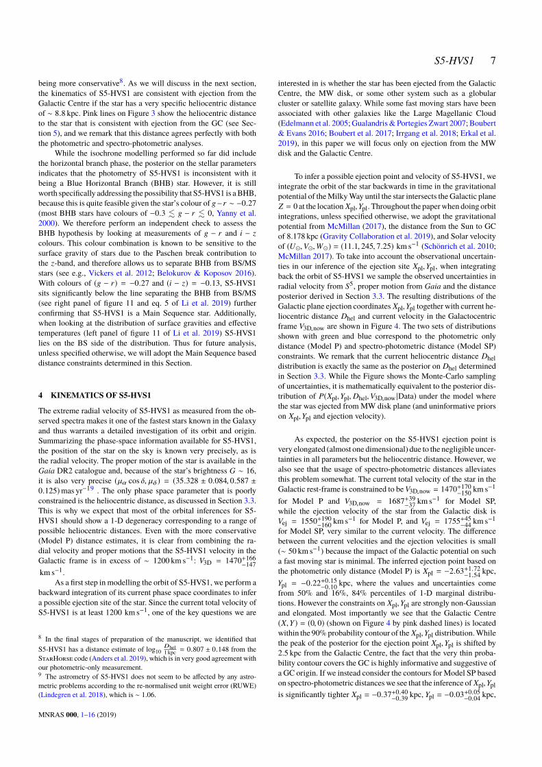
Figure 2. Spectral energy distribution (SED) of S5-HVS1 from GALEX,Gaia, SkyMapper, DES, 2MASS and WISE photometry. The blue curve isthe black-body spectrum with temperature of 10000K. The red line showsthe SED from the best-fit MIST isochrone model. The magnitudes in thedata and model were not extinction corrected.
this orbital motion would be negligible compared to the observedRV. Therefore most of the observed radial velocity must be causedby the motion through the Galaxy.
3.3 Photometry
S5-HVS1 was targeted by S5 as a blue star with −0.4 < g− r < 0.1,which makes it a possible BHB or BS. In this Section we assess thephotometric properties of S5-HVS1 by collecting its photometryacross multiple wavelengths and fitting these data with an isochronemodel.
As S5-HVS1 is quite bright, Gaia G ∼ 16, it is detected in alarge number of different surveys. Here we take the data from DESDR1 (Abbott et al. 2018), 2MASS (Skrutskie et al. 2006), AllWISE(Wright et al. 2010), SkyMapper DR1.1 (Wolf et al. 2018), GALEX(Martin et al. 2005; Bianchi et al. 2017) andGaiaDR2 (Brown et al.2018; Evans et al. 2018). Figure 2 shows all S5-HVS1 magnitudes(converted when needed from Vega to AB magnitude system) asa function of the effective wavelength of the corresponding filterwith standard errors. The SED is clearly indicative of a hot starwith temperature ∼ 10000K. The red line shows the photometryfrom the best fit isochrone model in the observed filters that wedescribe below. The blue line shows a black body spectrum with atemperature of 10000K.
To model the photometry of S5-HVS1 we use the MISTisochrones (Dotter 2016; Choi et al. 2016, version 1.2) and to inter-polate between isochrones we use the isochrones software (Mor-ton 2015, version 2.0.1)6. The data that we model are the observedmagnitudes mi where i corresponds to the i-th band. The isochronesprovide us with absolute magnitudes, surface gravities and effec-tive temperatures as a function of stellar age, mass, metallicity and
6 ForGaiaGBP,GRP magnitudes we use the band-passes defined byWeiler(2018).
Table 2. The parameters measured from fitting MIST isochrones to the S5-HVS1 SED (Model P) and by combining SED constraints with spectroscopicconstraints (Model SP).
Parameter Value Value unitPhotometric Spectro-Photometric
Mass 1.90+0.25−0.28 2.35+0.06
−0.06 M�log10 age 8.36+0.32
−0.46 7.72+0.25−0.33 dex
[Fe/H] −0.2+0.2−0.3 0.3+0.1
−0.1 dexm-M 14.21+0.37
−0.43 14.68+0.07−0.07 mag
σsys 0.04+0.01−0.01 0.03+0.01
−0.01 mag
band-pass M(age,M, [Fe/H], i). Assuming Gaussian uncertaintiesof observed magnitudes, our model is
mi ∼ N(M(age,M, [Fe/H], i)+
+ 5 log10 Dhel − 5 + kiE(B − V),√σ2i+ σ2
sys
),
(1)
where σi is the uncertainty on the magnitude measurement in bandi, σsys is an additional (systematic) scatter around the model, Dhelis the heliocentric distance to the star, and ki is the extinction co-efficient7 in the filter i. On top of the purely photometric modeldescribed in Eq. 1 (we label it Model P), we also consider a model(labelled Model SP) where we complement Eq. 1 with the con-straints on log g, Teff and [Fe/H] from the spectroscopic analysis(see Section 3.1), assuming they are normally distributed (i.e. wemultiply the likelihood byGaussian terms for log g,Teff and [Fe/H]).
We adopt generically uninformative priors for the parameters:uniform distribution on (linear) age ∼ U(105, 1.2 × 10¹⁰), SalpeterIMF prior for the stellar mass fromM = 0.1M� toM = 5M� ,uniform prior on metallicity [Fe/H] ∼ U(−4, 0.5), and a uniformprior on distance modulus 5 log10 Dhel−5 ∼ U(10, 20) correspond-ing to a 1/D2 spatial density prior from 1 kpc to 100 kpc. For theextinction, we adopt a prior around the Schlegel et al. (1998) valueE(B − V) ∼ U(0.3ESFD, 3ESFD). The posterior of the model issampled using the nested sampling MultiNest algorithm (Feroz &Hobson 2008; Buchner et al. 2014).
The posterior of the model parameters is shown in Figure 3;blue contours and curves for Model P and green for Model SP.Focusing on the Model P first, we notice that as expected fromphotometric only data there are considerable degeneracies betweenmass, age, metallicity and distance of the star. The summary ofparameters for Model P is provided in Table 2. The age of the staris consistent with a broad range of ages up to 500Myr. The massof the star is inferred to be 1.9 ± 0.25M� . The distance to thestar is constrained to be log10
Dhel1kpc = 0.836 ± 0.083, putting it in
the range of between ∼ 4.5 and 10 kpc from the Sun. We noticethat this distance corresponds to a parallax of πphot ∼ 0.14maswhich is consistent within 2 sigma with the negative Gaia parallaxmeasurement πGaia = −0.042 ± 0.091mas that was not used inthe fit. The systematic error for the photometry is determined bythe model to be σsys = 0.04 ± 0.01 showing that there is no largediscrepancy between isochrone models and data.
Thematch between the data and the isochronemodel across the
7 Taken from http://www.mso.anu.edu.au/~brad/filters.html
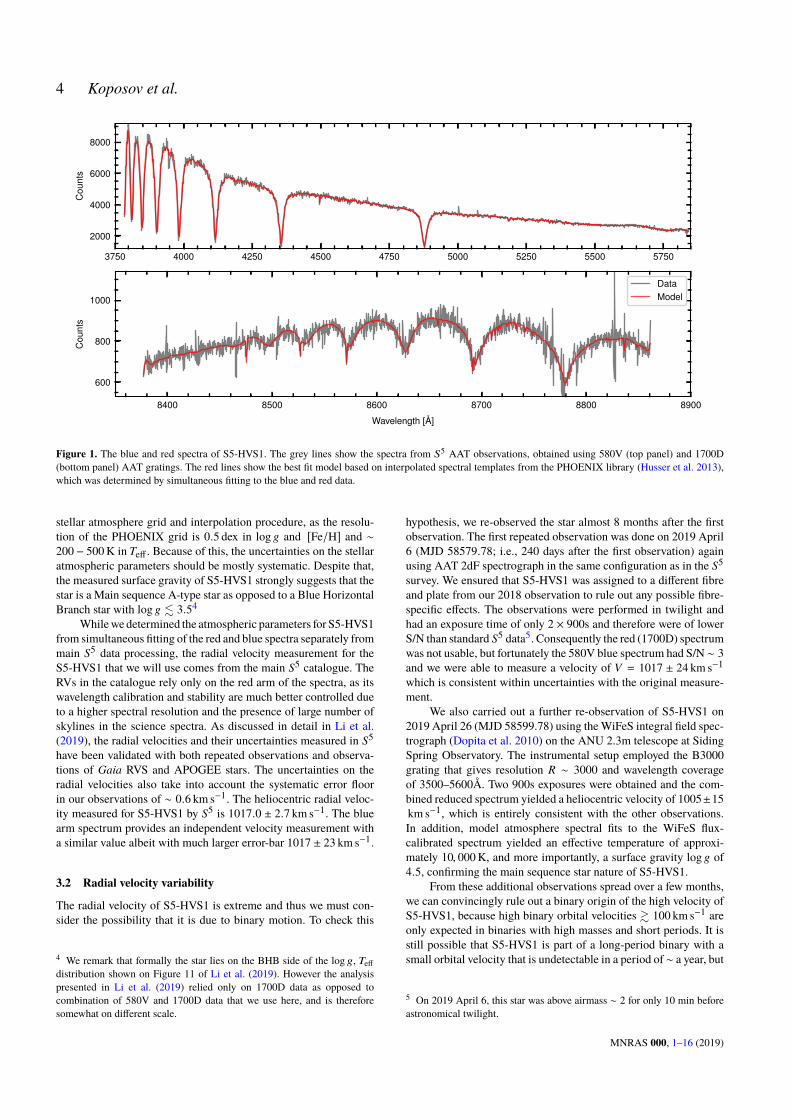
Figure 3. The posterior on stellar parameters of S5-HVS1 from fitting MIST isochrones to the SED data only (blue) and the SED data combined with theprior on stellar atmospheric parameters from spectroscopic analysis (green). The red points with error-bars are showing the best-fit measurement of stellaratmospheric parameters from the analysis of the AAT spectra using rvspecfit. The pink lines on several panels identify the heliocentric distance to the starthat is consistent with the Galactocentric origin (see Section 5). The contour levels in the 2-D marginal distributions corresponds to the 68%, 95% and 99.7%of posterior volumes.
wavelengths is well demonstrated by Figure 2. Red pointswith error-bars shown onmultiple panels of Figure 3mark the parameter valuesmeasured from spectroscopic analysis of S5-HVS1 (Section 3.1).The measurements from photometric data only are broadly consis-tent with the spectroscopic analysis, as the error-bars overlap withthe high probability parts of the posterior. Although there is possi-bly a small discrepancy in temperature of ∼ 200K and/or [Fe/H]of ∼ 0.2 dex between purely spectroscopic and photometric mea-surements, we believe this level of disagreement is well within thesystematic errors of our spectroscopic and isochrone modelling.
Since the photometric and spectroscopic analyses are consis-tent, we also show in the Figure the posterior from the combi-nation of the spectroscopic and photometric analyses (Model SP)as green contours. As expected, the combination of the datasetsshrinks the posteriors considerably, i.e. the combined mass estimateis 2.35±0.06M� and distance estimate is log Dhel
1kpc = 0.936±0.015.The posterior estimates for these and other parameters from theModel SP are also provided in Table 2. Throughout the paper weuse both the photometric and photometric+spectroscopic sets of es-timates, where we will interpret the photometric-only constraints as
MNRAS 000, 1–16 (2019)
S5-HVS1 7
being more conservative8. As we will discuss in the next section,the kinematics of S5-HVS1 are consistent with ejection from theGalactic Centre if the star has a very specific heliocentric distanceof ∼ 8.8 kpc. Pink lines on Figure 3 show the heliocentric distanceto the star that is consistent with ejection from the GC (see Sec-tion 5), and we remark that this distance agrees perfectly with boththe photometric and spectro-photometric analyses.
While the isochrone modelling performed so far did includethe horizontal branch phase, the posterior on the stellar parametersindicates that the photometry of S5-HVS1 is inconsistent with itbeing a Blue Horizontal Branch (BHB) star. However, it is stillworth specifically addressing the possibility that S5-HVS1 is aBHB,because this is quite feasible given the star’s colour of g−r ∼ −0.27(most BHB stars have colours of −0.3 . g − r . 0, Yanny et al.2000). We therefore perform an independent check to assess theBHB hypothesis by looking at measurements of g − r and i − zcolours. This colour combination is known to be sensitive to thesurface gravity of stars due to the Paschen break contribution tothe z-band, and therefore allows us to separate BHB from BS/MSstars (see e.g., Vickers et al. 2012; Belokurov & Koposov 2016).With colours of (g − r) = −0.27 and (i − z) = −0.13, S5-HVS1sits significantly below the line separating the BHB from BS/MS(see right panel of figure 11 and eq. 5 of Li et al. 2019) furtherconfirming that S5-HVS1 is a Main Sequence star. Additionally,when looking at the distribution of surface gravities and effectivetemperatures (left panel of figure 11 of Li et al. 2019) S5-HVS1lies on the BS side of the distribution. Thus for future analysis,unless specified otherwise, we will adopt the Main Sequence baseddistance constraints determined in this Section.
4 KINEMATICS OF S5-HVS1
The extreme radial velocity of S5-HVS1 as measured from the ob-served spectra makes it one of the fastest stars known in the Galaxyand thus warrants a detailed investigation of its orbit and origin.Summarizing the phase-space information available for S5-HVS1,the position of the star on the sky is known very precisely, as isthe radial velocity. The proper motion of the star is available in theGaia DR2 catalogue and, because of the star’s brightness G ∼ 16,it is also very precise (µα cos δ, µδ) = (35.328 ± 0.084, 0.587 ±0.125)mas yr−19 . The only phase space parameter that is poorlyconstrained is the heliocentric distance, as discussed in Section 3.3.This is why we expect that most of the orbital inferences for S5-HVS1 should show a 1-D degeneracy corresponding to a range ofpossible heliocentric distances. Even with the more conservative(Model P) distance estimates, it is clear from combining the ra-dial velocity and proper motions that the S5-HVS1 velocity in theGalactic frame is in excess of ∼ 1200 km s−1: V3D = 1470+166
−147km s−1.
As a first step in modelling the orbit of S5-HVS1, we perform abackward integration of its current phase space coordinates to infera possible ejection site of the star. Since the current total velocity ofS5-HVS1 is at least 1200 km s−1, one of the key questions we are
8 In the final stages of preparation of the manuscript, we identified thatS5-HVS1 has a distance estimate of log10
Dhel1 kpc = 0.807 ± 0.148 from the
StarHorse code (Anders et al. 2019), which is in very good agreement withour photometric-only measurement.9 The astrometry of S5-HVS1 does not seem to be affected by any astro-metric problems according to the re-normalised unit weight error (RUWE)(Lindegren et al. 2018), which is ∼ 1.06.
interested in is whether the star has been ejected from the GalacticCentre, the MW disk, or some other system such as a globularcluster or satellite galaxy. While some fast moving stars have beenassociated with other galaxies like the Large Magellanic Cloud(Edelmann et al. 2005;Gualandris&Portegies Zwart 2007; Boubert& Evans 2016; Boubert et al. 2017; Irrgang et al. 2018; Erkal et al.2019), in this paper we will focus only on ejection from the MWdisk and the Galactic Centre.
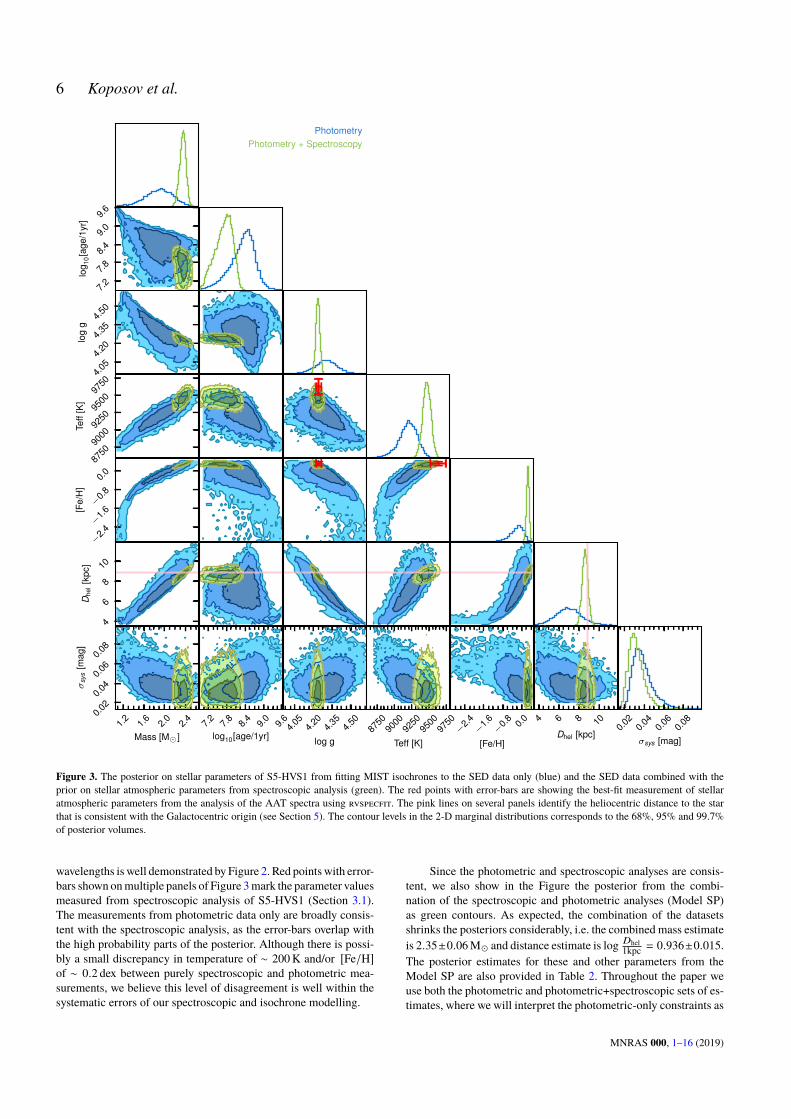
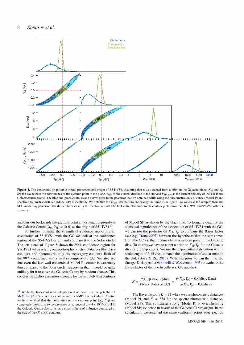
To infer a possible ejection point and velocity of S5-HVS1, weintegrate the orbit of the star backwards in time in the gravitationalpotential of theMilkyWay until the star intersects the Galactic planeZ = 0 at the location Xpl,Ypl. Throughout the paperwhen doing orbitintegrations, unless specified otherwise, we adopt the gravitationalpotential from McMillan (2017), the distance from the Sun to GCof 8.178 kpc (Gravity Collaboration et al. 2019), and Solar velocityof (U�,V�,W�) = (11.1, 245, 7.25) km s−1 (Schönrich et al. 2010;McMillan 2017). To take into account the observational uncertain-ties in our inference of the ejection site Xpl,Ypl, when integratingback the orbit of S5-HVS1 we sample the observed uncertainties inradial velocity from S5, proper motion from Gaia and the distanceposterior derived in Section 3.3. The resulting distributions of theGalactic plane ejection coordinates Xpl,Ypl together with current he-liocentric distance Dhel and current velocity in the Galactocentricframe V3D,now are shown in Figure 4. The two sets of distributionsshown with green and blue correspond to the photometric onlydistance (Model P) and spectro-photometric distance (Model SP)constraints. We remark that the current heliocentric distance Dheldistribution is exactly the same as the posterior on Dhel determinedin Section 3.3. While the Figure shows the Monte-Carlo samplingof uncertainties, it is mathematically equivalent to the posterior dis-tribution of P(Xpl,Ypl,Dhel,V3D,now |Data) under the model wherethe star was ejected from MW disk plane (and uninformative priorson Xpl,Ypl and ejection velocity).
As expected, the posterior on the S5-HVS1 ejection point isvery elongated (almost one dimensional) due to the negligible uncer-tainties in all parameters but the heliocentric distance. However, wealso see that the usage of spectro-photometric distances alleviatesthis problem somewhat. The current total velocity of the star in theGalactic rest-frame is constrained to beV3D,now = 1470+170
−150 km s−1
for Model P and V3D,now = 1687+39−37 km s−1 for Model SP,
while the ejection velocity of the star from the Galactic disk isVej = 1550+190
−160 km s−1 for Model P, and Vej = 1755+45−44 km s−1
for Model SP, very similar to the current velocity. The differencebetween the current velocities and the ejection velocities is small(∼ 50 km s−1) because the impact of the Galactic potential on sucha fast moving star is minimal. The inferred ejection point based onthe photometric only distance (Model P) is Xpl = −2.63+1.72
−1.54 kpc,Ypl = −0.22+0.15
−0.10 kpc, where the values and uncertainties comefrom 50% and 16%, 84% percentiles of 1-D marginal distribu-tions. However the constraints on Xpl,Ypl are strongly non-Gaussianand elongated. Most importantly we see that the Galactic Centre(X,Y ) = (0, 0) (shown on Figure 4 by pink dashed lines) is locatedwithin the 90%probability contour of the Xpl,Ypl distribution.Whilethe peak of the posterior for the ejection point Xpl,Ypl is shifted by2.5 kpc from the Galactic Centre, the fact that the very thin proba-bility contour covers the GC is highly informative and suggestive ofa GC origin. If we instead consider the contours for Model SP basedon spectro-photometric distanceswe see that the inference of Xpl,Yplis significantly tighter Xpl = −0.37+0.40
−0.39 kpc, Ypl = −0.03+0.05−0.04 kpc,
MNRAS 000, 1–16 (2019)
8 Koposov et al.
PhotometryPhotometry+Spectroscopy
−0.4
−0.2
0.0
0.2
0.4
Ypl
[kpc
]
4
6
8
10
Dhe
l[k
pc]
−5.0 −2.5 0.0 2.5Xpl [kpc]
1250
1500
1750
2000
V3D
,now
[km
/s]
−0.4 −0.2 0.0 0.2 0.4Ypl [kpc]
4 6 8 10Dhel [kpc]
1250 1500 1750 2000V3D,now [km/s]
Figure 4. The constraints on possible orbital properties and origin of S5-HVS1, assuming that it was ejected from a point in the Galactic plane. Xpl and Yplare the Galactocentric coordinates of the ejection point in the plane. Dhel is the current distance to the star andV3D,now is the current velocity of the star in theGalactocentric frame. The blue and green contours and curves refer to the posterior that we obtained while using the photometric only distance (Model P) andspectro-photometric distance (Model SP) respectively. We note that the Dhel distributions are exactly the same as in Figure 3 as we reuse the samples from theSED modelling posterior. The dashed lines identify the location of the Galactic Centre. The lines in the contour plots show the 68%, 95% and 99.7% posteriorvolumes.
and thus our backwards integrations point almost unambiguously atthe Galactic Centre (Xpl,Ypl) = (0, 0) as the origin of S5-HVS110.
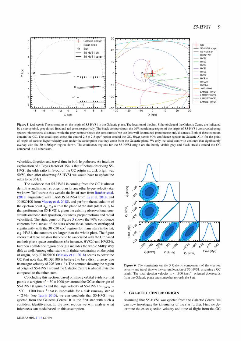
To further illustrate the strength of evidence supporting anassociation of S5-HVS1 with the GC we look at the confidenceregion of the S5-HVS1 origin and compare it to the Solar circle.The left panel of Figure 5 shows the 90% confidence region forS5-HVS1 when relying on spectro-photometric distances (the blackcontour), and photometric only distances (grey contour). Both ofthe 90% confidence limits well encompass the GC. We also seethat even the less well constrained Model P contour is extremelythin compared to the Solar circle, suggesting that it would be quiteunlikely for it to cover the Galactic Centre by random chance. Thisconclusion applies evenmore strongly for theminutely thin contours
10 While the backward orbit integration done here uses the potential ofMcMillan (2017), which does not include the SMBH in the Galactic Centre,we have verified that the constraints on the ejection point (Xpl,Ypl) arecompletely insensitive to the presence or absence of a ∼ 4 × 10⁶ M� BH inthe Galactic Centre due to its very small sphere of influence compared tothe size of the (Xpl,Ypl) contours.
of Model SP as shown by the black line. To formally quantify thestatistical significance of the association of S5-HVS1 with the GC,we can use the posterior on Xpl, Ypl to compute the Bayes factor(see e.g. Trotta 2007) between the hypothesis that the star comesfrom the GC vs. that it comes from a random point in the Galacticdisk. To do this we have to adopt a prior on Xpl,Ypl for the Galacticdisk origin hypothesis. We use the exponential distribution with ascale length of 2.15 kpc, to match the distribution of stellar mass inthe disk (Bovy & Rix 2013). With this prior we can then use theSavage-Dickey ratio (Verdinelli &Wasserman 1995) to evaluate theBayes factor of the two hypotheses: GC and disk.
K =P(GC|Data)P(disk|Data)
π(disk)π(GC) =
P(Xpl,Ypl = 0, 0|disk,Data)π(Xpl,Ypl = 0, 0|disk)
.The Bayes factor is K = 81when we use photometric distances
(Model P), and K = 354 for the spectro-photometric distances(Model SP). This constitutes strong (Model P) or overwhelming(Model SP) evidence in favour of the Galactic Centre origin. In thecalculation, we assumed the same (uniform) priors over ejection
Figure 5. Left panel: The constraints on the origin of S5-HVS1 in the Galactic plane. The location of the Sun, Solar circle and the Galactic Centre are indicatedby a star symbol, grey dotted line, and red cross respectively. The black contour shows the 90% confidence region of the origin of S5-HVS1 constructed usingspectro-photometric distances, while the grey contour shows the constraints if we use less well determined photometric only distances. Both of these contourscontain the GC. The small inset shows the central 2.5 × 2.5 kpc2 region around the GC. Right panel: 90% confidence regions in Galactic X,Y for the pointof origin of various hyper-velocity stars under the assumption that they come from the Galactic plane. We only included stars with contours that significantlyoverlap with the 30 × 30 kpc2 region shown. The confidence regions for the S5-HVS1 origin are the barely visible grey and black streaks around the GCcompared to all other stars.
velocities, direction and travel time in both hypotheses. An intuitiveexplanation of a Bayes factor of 354 is that if before observing S5-HVS1 the odds ratio in favour of the GC origin vs. disk origin was50/50, then after observing S5-HVS1 we would have to update theodds to be 354/1.
The evidence that S5-HVS1 is coming from the GC is almostdefinitive and is much stronger than for any other hyper-velocity starwe know. To illustrate this we take the list of stars fromBoubert et al.(2018, augmented with LAMOST-HVS4 from Li et al. 2018, andJ01020100 fromMassey et al. 2018), and perform the calculation ofthe ejection point Xpl,Ypl within the plane of the disk (identically tothat performed on S5-HVS1), given the existing observational con-straints on those stars (position, distances, proper motions and radialvelocities). The right panel of Figure 5 shows the 90% confidencecontours for a subset of the stars where those contours overlappedsignificantly with the 30× 30 kpc2 region (for many stars in the list,e.g. HVS1, the contours are larger than the whole plot). The figureshows that there are stars that could be associated with the GC basedon their phase space coordinates (for instance, HVS20 and HVS24),but their confidence region of origin includes the whole Milky Waydisk as well. Among other stars with tighter constraints on the pointof origin, only J01020100 (Massey et al. 2018) seems to cover theGC (but note that J01020100 is believed to be a disk runaway dueits meagre velocity of 296 km s−1). The contour showing the regionof origin of S5-HVS1 around the Galactic Centre is almost invisiblecompared to the other stars.
Concluding this section, based on strong orbital evidence thatpoints at a region of ∼ 50×1000 pc2 around the GC as the origin ofS5-HVS1 (Figure 5) and the large velocity of S5-HVS1 V3D,now ∼1500 − 1700 km s−1 that is impossible for a disk runaway star of∼ 2M� (see Tauris 2015), we can conclude that S5-HVS1 wasejected from the Galactic Centre. It is the first star with such aconfident identification. In the next section we will analyse whatinferences can made based on this assumption.
−384
−382
−380
Vy
[km
/s]
−1576
−1568
Vz
[km
/s]
−790−78
5−78
0
Vx [km/s]
4.78
4.80
4.82
Tim
e[M
yr]
−384−38
2−38
0
Vy [km/s]−15
76
−1568
Vz [km/s]
4.78
4.80
4.82
Time [Myr]
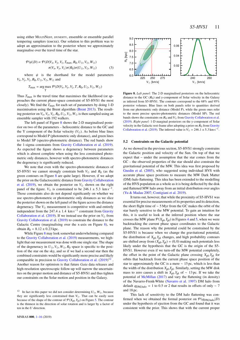
Figure 6. The constraints on the 3 Galactic components of the ejectionvelocity and travel time to the current location of S5-HVS1, assuming a GCorigin. The total ejection velocity is ∼ 1800 km s−1 oriented downwardsfrom the Galactic plane and somewhat towards the Sun.
5 GALACTIC CENTRE ORIGIN
Assuming that S5-HVS1 was ejected from the Galactic Centre, wecan now investigate the kinematics of the star further. First we de-termine the exact ejection velocity and time of flight from the GC
MNRAS 000, 1–16 (2019)
10 Koposov et al.
required to match the observations of S5-HVS1, by ejecting the starfrom the centre of the MW in the potential of McMillan (2017)(without considering the potential of the SMBH itself). This givesa prediction of α, δ, µα, µδ, RV,Dhel as a function of the ejectionvelocities Vx,Vy,Vz and travel time T . We then write a Normal like-lihood function using the observed position, distance, propermotionand RV of S5-HVS1 and their uncertainties (we use a Gaussian ap-proximation to the log10 Dhel posterior from Section 3.3). We adoptnon-informative uniform priors on all the parameters and then sam-ple the posterior using an ensemble sampler. Figure 6 shows the pos-terior. This model implies an ejection speed of 1798.6± 3.1 km s−1
with the z-component of the velocity being the largest and a totaltravel time from theGC to the current position of 4.801±0.009 Myr.We note that the constraints on the ejection velocities are now muchtighter compared to Figure 4. The reason for this is that postulatingthat the star is coming from the GC strongly constrains the currentdistance to S5-HVS1 to be Dhel = 8884± 11 pc and thus makes ourspectro-photometric measurement mostly irrelevant.11. We also re-mark that the measured ejection speed of 1798.6± 3.1 km s−1 fromthe GC was computed while ignoring the potential of the SMBH,and thus represents the ejection velocity outside the sphere of in-fluence of the black hole (& 1 pc). The actual ejection speed ofthe star depends on how close to the BH the ejection happened,and could easily be as high as ∼ 8000 km s−1 if the ejection hap-pened at a distance of 100 AU from the BH. Assuming a GC originalso allows us to improve the proper motion precision from theone delivered by Gaia µα cos δ = 35.333 ± 0.081 mas yr−1 andµδ = 0.617 ± 0.011 mas yr−1. While the µα cos δ precision did notimprove much, the error-bar on the predicted µδ is 8 times smallerthan Gaia’s. Since the full phase space position of S5-HVS1 be-comes very precise when we adopt the GC origin hypothesis, wecan look at the geometric position of S5-HVS1 in the Galaxy. Thisis shown in Figure 7. We see that as expected, S5-HVS1 is mostlymoving downwards away from the disk, and that the Sun, Galac-tic Centre and S5-HVS1 form an almost equilateral triangle with∼ 8 − 9 kpc edges.
In this section we will further use the phase space observationsof S5-HVS1 to constrain the gravitational potential of the MW,location and kinematics of the Sun in the Galaxy, and assess thepossible connection of S5-HVS1 to the stars in the vicinity of SgrA*.
5.1 Constraining the position and motion of the Sun
Figure 5 shows that the association of S5-HVS1 with the GC cru-cially depends on the relative geometry between the Sun and theGalactic Centre. For example, a small adjustment of the distancefrom the Sun to the Galactic Centre (R0) could easily shift thehigh probability contour P(Xpl,Ypl) away from the GC. Thereforeassuming that S5-HVS1 originates in the GC constrains R0 and pos-sibly other Galactic parameters. The idea of constraining the Solarmotion as well as the distances to the Galactic Centre have beendiscussed previously, most notably by Hattori et al. (2018b). To de-termine these constraints, we construct a forward model where weeject the star from the GC with velocity Vx,Vy,Vz and let it travelin the Galactic potential of McMillan (2017) for the time T . Wethen observe it from the Sun located at a distance of R0 from the
11 Given a star ejected from the Galactic Centre, it is enough to knowaccurately just the position of the star on the sky and proper motion toexactly determine its heliocentric distance and radial velocity.
−10
−5
0
5
10
Y[k
pc]
−10 −5 0 5 10X [kpc]
−15
−10
−5
0
5
Z[k
pc]
−5 0 5 10Y [kpc]
SunGCS5-HVS1
Figure 7. The location and direction of motion of S5-HVS1 in the Galaxyassuming aGalacticCentre origin. Three panels showdifferent projections inGalactic Cartesian coordinates. The location of the Sun, theGC and the Solarcircle are marked by the orange star, red cross and grey circle respectively.The arrow shows the direction of S5-HVS1’s velocity in the correspondingprojection. The length of the arrow corresponds to the distance traveled bythe star in 4Myr.
Galactic Centre and moving with the velocity U�,V�,W� km s−1
(this includes both the speed of the Local Standard of Rest and thepeculiar velocity of the Sun). The likelihood of the model is thenconstructed using the observed 6-D phase measurements of S5-HVS1: position, proper motion, distance and radial velocity. Thisleads to the following posterior distribution:
where ψ is the shorthand for all the model parametersVx,Vy,Vz,T, R0,U�,V�,W� . For this model we focus on con-straining R0 and V� , so we adopt broad uninformative priors onthe distance of the Sun to the Galactic Centre R0
1 kpc ∼ U(6, 9),and V�
1 km s−1 ∼ U(200, 290) and informed Normal priors on theother two components of Solar velocity U�
1 km s−1 ∼ N(11.1, 0.5),W�
1 km s−1 ∼ N(7.25, 0.5) (Schönrich et al. 2010). For the rest ofparameters Vx,Vy,Vz,T we adopt uninformative uniform priors. Inprinciple the model that we have described has a valid posterior thatwe could sample. However, we have discovered that this posterioris extremely degenerate along one dimension and narrow in anotherdimension. This is in fact a direct consequence of the elongatedcontour shape for the constraint on the ejection point Xpl,Ypl seen inFigure 5. This contour shape and the fact that simultaneous changesof V� and R0 give two degrees of freedom for "moving" the highprobability contour in (Xpl,Ypl) space while still covering the GCexplains the long degeneracy ridge in the posterior. Furthermore theposterior is also extremely narrow along the time axis, as the orbitneeds to pass very close to the precisely known observed positionon the sky. It turns out that those features of the posterior make it ex-tremely challenging to sample, so we were unable to do it efficiently
MNRAS 000, 1–16 (2019)
S5-HVS1 11
using either MultiNest, dynesty, ensemble or ensemble paralleltempering samplers (emcee). Our solution to this problem was toadopt an approximation to the posterior where we approximatelymarginalise over the travel time of the star.
where ψ is the shorthand for the model parametersVx,Vy,Vz, R0,U�,V�,W� and
Tmax = arg maxT
P(D |Vx,Vy,Vz,T, R0,U�,V�,W�)
Thus Tmax is the travel time that maximises the likelihood (or ap-proaches the current phase-space constraint of S5-HVS1 the mostclosely). We find the Tmax for each set of parameters by doing 1-Dmaximisation using the Brent algorithm (Brent 2013). The result-ing posterior onVx,Vy,Vz, R0,U�,V�,W� is then sampled using anensemble sampler with 192 walkers.
The left panel of Figure 8 shows the 2-D marginalised poste-rior on two of the parameters – heliocentric distance to the GC andthe Y component of the Solar velocity (V�). As before blue linescorrespond to Model P (photometric only distance), and green linesto Model SP (spectro-photometric distance). The red bands showthe 1-sigma constraints from Gravity Collaboration et al. (2019).As expected the figure shows a degeneracy between parameterswhich is almost complete when using the less constrained photo-metric only distances, however with spectro-photometric distancesthe degeneracy is significantly reduced.
We note that even with the spectro-photometric distances ofS5-HVS1 we cannot strongly constrain both V� and R0 (as thegreen contours on Figure 8 are quite large). However, if we adoptthe prior on the Galactocentric distance from Gravity Collaborationet al. (2019), we obtain the posterior on V� shown on the rightpanel of the figure. V� is constrained to be 246.1 ± 5.3 km s−1.Those constraints also do not depend significantly on whether weuse spectro-photometric or photometric only distances as we slicethe posterior shown on the left panel of the figure across the distancedegeneracy. The V� measurement is competitive with and entirelyindependent from the 247.4 ± 1.4 km s−1 constraint from GravityCollaboration et al. (2019). If we instead use the prior on V� fromGravity Collaboration et al. (2019) to constrain the distance to theGalactic Centre (marginalising over the x-axis on Figure 8), weobtain R0 = 8.12 ± 0.23 kpc.
While Figure 8 may look somewhat underwhelming comparedto the Gravity Collaboration et al. (2019) measurements, we high-light that our measurement was done with one single star. The shapeof the degeneracy in U�,V�,W�, R0 space is specific to the posi-tion of the star on the sky, and so if we had a second star then thecombined constraints would be significantly more precise and likelycomparable in precision to Gravity Collaboration et al. (2019)12 .Another reason for optimism is that future Gaia data releases andhigh-resolution spectroscopic follow-up will narrow the uncertain-ties on the proper motion and distance of S5-HVS1 and thus tightenour constraints on the Solar motion and position in the Galaxy.
12 In fact in this paper we did not consider determiningU�,W� , becausethey are significantly less constrained than V� . That can be easily seenbecause of the shape of the contour of P(Xpl,Ypl) on Figure 5. The contouris the thinnest in the direction of solar rotation and is larger by a factor often in theU direction.
225 250 275V� [km/s]
6.0
6.5
7.0
7.5
8.0
8.5
9.0
R0
[kpc
]
240 260V� [km/s]
0.02
0.04
0.06
Figure 8. Left panel: The 2-D marginalised posteriors on the heliocentricdistance to the GC (R0) and y-component of Solar velocity in the Galaxyas inferred from S5-HVS1. The contours correspond to the 68% and 95%posterior volumes. Blue lines on both panels refer to quantities derivedfrom our photometric only distance (Model P), while the green ones referto the more precise spectro-photometric distances (Model SP). The redbands shows the constraints on R0 andV� from Gravity Collaboration et al.(2019). Right panel: 1-D marginal posteriors on the y-component of Solarvelocity in the Galactic rest-frame after adopting a prior on R0 from GravityCollaboration et al. (2019). The inferred value isV� = 246.1 ± 5.3 km s−1.
5.2 Constraints on the Galactic potential
As we showed in the previous section, S5-HVS1 strongly constrainsthe Galactic position and velocity of the Sun. On top of that weexpect that – under the assumption that the star comes from theGC – the observed properties of the star should also constrain thegravitational potential of the MW. This idea was first proposed byGnedin et al. (2005), who suggested using individual HVS withaccurate phase space positions to measure the MW Dark Matter(DM) halo flattening. This idea has been extended to the modellingof the HVS population as a whole as it is being deflected by the diskand flattened MW halo away from an initial distribution over angles(Yu & Madau 2007; Contigiani et al. 2019).
It turns out, however, that while the proximity of S5-HVS1 wasessential for precisemeasurements of its properties and its detection,the short flight time of ∼ 5Myr from the GC makes the orbit of thestar barely sensitive to the MW potential. To gain an intuition forthis, it is useful to look at the inferred position where the starcrosses the MW plane P(Xpl,Ypl) in Figures 4 and 5, when we werebacktracking the current phase space coordinates to the Galacticplane. The reason why the potential could be constrained by theS5-HVS1 is because when we change the gravitational potential,the distribution of Xpl,Ypl changes, and high probability contoursare shifted away from (Xpl,Ypl) = (0, 0)making such potentials lesslikely under the hypothesis that the GC is the origin of the S5-HVS1. However even if we turn-off the MW potential completely,the offset in the point of the Galactic plane crossing Xpl,Ypl fororbits that backtrack from the current phase space position of thestar to approximately the GC is a mere ∼ 15 pc, which is less thanthe width of the distribution Xpl,Ypl. Similarly, setting the MW diskmass to zero causes a shift in Xpl,Ypl of ∼ 13 pc. If we take thepotential of McMillan (2017) and vary the flattening (in density)of the Navarro-Frenk-White (Navarro et al. 1997) DM halo fromdefault qDM,halo = 1 to 0.5 or 2 that results in offsets of only ∼ 7and 18 pc.
This lack of sensitivity to the DM halo flattening was con-firmed when we obtained the formal posterior on P(qDM,halo |D)under the hypothesis of ejection from the GC and found that it wasconsistent with the prior. This shows that with the current proper
MNRAS 000, 1–16 (2019)
12 Koposov et al.
motion precision, S5-HVS1 cannot yet be used to constrain theMWgravitational potential. One additional reason for the current lack ofconstraining power from S5-HVS1 is that, because we do not knowthe actual ejection velocity from the BH, we do not constrain thetotal deceleration of the star, but only deviations of the trajectoryfrom a straight line. For meaningful potentials consistent with theexisting data, the deviations from a straight line for a∼ 2000 km s−1
star flying for ∼ 5Myr are within a few tens of parsecs (listed above)and thus within the current uncertainties of the S5-HVS1 trajectory.With the improvement in proper motion precision from future Gaiadata we expect, however, that constraints on the MW halo flatteningwill be possible.
5.3 S5-HVS1 ejection by Sgr A*
Given an almost certain GC origin of S5-HVS1, here we discusspossible implications for the ejection by Sgr A*. We focus on theHills (1988) mechanism involving a three-body interaction of astellar binary with the SMBH leading to one star being ejected.There are other mechanisms involving binary black holes (Yu &Tremaine 2003; Levin 2006) and a SMBH surrounded by a clusterof stellar mass black holes (O’Leary & Loeb 2008), and we willdiscuss some of them later.
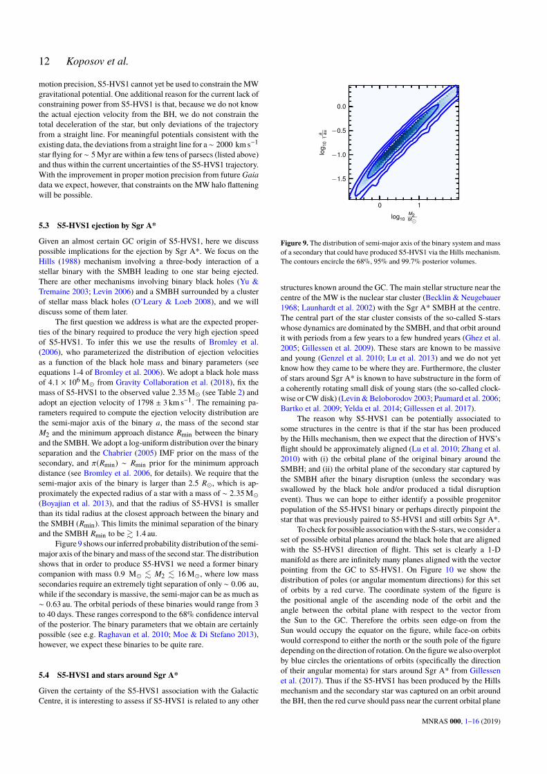
The first question we address is what are the expected proper-ties of the binary required to produce the very high ejection speedof S5-HVS1. To infer this we use the results of Bromley et al.(2006), who parameterized the distribution of ejection velocitiesas a function of the black hole mass and binary parameters (seeequations 1-4 of Bromley et al. 2006). We adopt a black hole massof 4.1 × 10⁶ M� from Gravity Collaboration et al. (2018), fix themass of S5-HVS1 to the observed value 2.35M� (see Table 2) andadopt an ejection velocity of 1798 ± 3 km s−1. The remaining pa-rameters required to compute the ejection velocity distribution arethe semi-major axis of the binary a, the mass of the second starM2 and the minimum approach distance Rmin between the binaryand the SMBH.We adopt a log-uniform distribution over the binaryseparation and the Chabrier (2005) IMF prior on the mass of thesecondary, and π(Rmin) ∼ Rmin prior for the minimum approachdistance (see Bromley et al. 2006, for details). We require that thesemi-major axis of the binary is larger than 2.5 R� , which is ap-proximately the expected radius of a star with a mass of ∼ 2.35M�(Boyajian et al. 2013), and that the radius of S5-HVS1 is smallerthan its tidal radius at the closest approach between the binary andthe SMBH (Rmin). This limits the minimal separation of the binaryand the SMBH Rmin to be & 1.4 au.
Figure 9 shows our inferred probability distribution of the semi-major axis of the binary andmass of the second star. The distributionshows that in order to produce S5-HVS1 we need a former binarycompanion with mass 0.9 M� . M2 . 16M� , where low masssecondaries require an extremely tight separation of only∼ 0.06 au,while if the secondary is massive, the semi-major can be as much as∼ 0.63 au. The orbital periods of these binaries would range from 3to 40 days. These ranges correspond to the 68% confidence intervalof the posterior. The binary parameters that we obtain are certainlypossible (see e.g. Raghavan et al. 2010; Moe & Di Stefano 2013),however, we expect these binaries to be quite rare.
5.4 S5-HVS1 and stars around Sgr A*
Given the certainty of the S5-HVS1 association with the GalacticCentre, it is interesting to assess if S5-HVS1 is related to any other
0 1
log10M2M�
−1.5
−1.0
−0.5
0.0
log 1
0a
1au
Figure 9. The distribution of semi-major axis of the binary system and massof a secondary that could have produced S5-HVS1 via the Hills mechanism.The contours encircle the 68%, 95% and 99.7% posterior volumes.
structures known around the GC. The main stellar structure near thecentre of the MW is the nuclear star cluster (Becklin & Neugebauer1968; Launhardt et al. 2002) with the Sgr A* SMBH at the centre.The central part of the star cluster consists of the so-called S-starswhose dynamics are dominated by the SMBH, and that orbit aroundit with periods from a few years to a few hundred years (Ghez et al.2005; Gillessen et al. 2009). These stars are known to be massiveand young (Genzel et al. 2010; Lu et al. 2013) and we do not yetknow how they came to be where they are. Furthermore, the clusterof stars around Sgr A* is known to have substructure in the form ofa coherently rotating small disk of young stars (the so-called clock-wise or CWdisk) (Levin&Beloborodov 2003; Paumard et al. 2006;Bartko et al. 2009; Yelda et al. 2014; Gillessen et al. 2017).
The reason why S5-HVS1 can be potentially associated tosome structures in the centre is that if the star has been producedby the Hills mechanism, then we expect that the direction of HVS’sflight should be approximately aligned (Lu et al. 2010; Zhang et al.2010) with (i) the orbital plane of the original binary around theSMBH; and (ii) the orbital plane of the secondary star captured bythe SMBH after the binary disruption (unless the secondary wasswallowed by the black hole and/or produced a tidal disruptionevent). Thus we can hope to either identify a possible progenitorpopulation of the S5-HVS1 binary or perhaps directly pinpoint thestar that was previously paired to S5-HVS1 and still orbits Sgr A*.
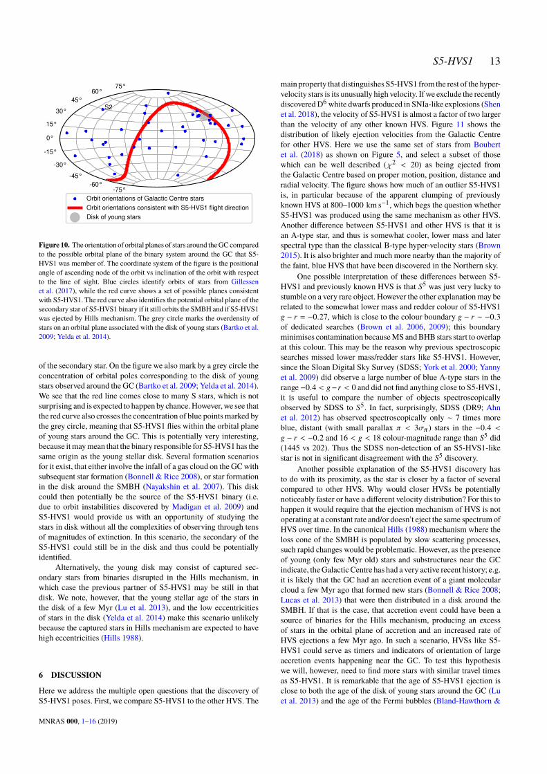
To check for possible associationwith the S-stars, we consider aset of possible orbital planes around the black hole that are alignedwith the S5-HVS1 direction of flight. This set is clearly a 1-Dmanifold as there are infinitely many planes aligned with the vectorpointing from the GC to S5-HVS1. On Figure 10 we show thedistribution of poles (or angular momentum directions) for this setof orbits by a red curve. The coordinate system of the figure isthe positional angle of the ascending node of the orbit and theangle between the orbital plane with respect to the vector fromthe Sun to the GC. Therefore the orbits seen edge-on from theSun would occupy the equator on the figure, while face-on orbitswould correspond to either the north or the south pole of the figuredepending on the direction of rotation.On the figurewe also overplotby blue circles the orientations of orbits (specifically the directionof their angular momenta) for stars around Sgr A* from Gillessenet al. (2017). Thus if the S5-HVS1 has been produced by the Hillsmechanism and the secondary star was captured on an orbit aroundthe BH, then the red curve should pass near the current orbital plane
MNRAS 000, 1–16 (2019)
S5-HVS1 13
-75°-60°
-45°
-30°
-15°
0°
15°
30°
45°60°
75°
S2
Orbit orientations of Galactic Centre starsOrbit orientations consistent with S5-HVS1 flight directionDisk of young stars
Figure 10. The orientation of orbital planes of stars around theGCcomparedto the possible orbital plane of the binary system around the GC that S5-HVS1 was member of. The coordinate system of the figure is the positionalangle of ascending node of the orbit vs inclination of the orbit with respectto the line of sight. Blue circles identify orbits of stars from Gillessenet al. (2017), while the red curve shows a set of possible planes consistentwith S5-HVS1. The red curve also identifies the potential orbital plane of thesecondary star of S5-HVS1 binary if it still orbits the SMBH and if S5-HVS1was ejected by Hills mechanism. The grey circle marks the overdensity ofstars on an orbital plane associated with the disk of young stars (Bartko et al.2009; Yelda et al. 2014).
of the secondary star. On the figure we also mark by a grey circle theconcentration of orbital poles corresponding to the disk of youngstars observed around the GC (Bartko et al. 2009; Yelda et al. 2014).We see that the red line comes close to many S stars, which is notsurprising and is expected to happen by chance.However,we see thatthe red curve also crosses the concentration of blue pointsmarked bythe grey circle, meaning that S5-HVS1 flies within the orbital planeof young stars around the GC. This is potentially very interesting,because itmaymean that the binary responsible for S5-HVS1has thesame origin as the young stellar disk. Several formation scenariosfor it exist, that either involve the infall of a gas cloud on the GCwithsubsequent star formation (Bonnell & Rice 2008), or star formationin the disk around the SMBH (Nayakshin et al. 2007). This diskcould then potentially be the source of the S5-HVS1 binary (i.e.due to orbit instabilities discovered by Madigan et al. 2009) andS5-HVS1 would provide us with an opportunity of studying thestars in disk without all the complexities of observing through tensof magnitudes of extinction. In this scenario, the secondary of theS5-HVS1 could still be in the disk and thus could be potentiallyidentified.
Alternatively, the young disk may consist of captured sec-ondary stars from binaries disrupted in the Hills mechanism, inwhich case the previous partner of S5-HVS1 may be still in thatdisk. We note, however, that the young stellar age of the stars inthe disk of a few Myr (Lu et al. 2013), and the low eccentricitiesof stars in the disk (Yelda et al. 2014) make this scenario unlikelybecause the captured stars in Hills mechanism are expected to havehigh eccentricities (Hills 1988).
6 DISCUSSION
Here we address the multiple open questions that the discovery ofS5-HVS1 poses. First, we compare S5-HVS1 to the other HVS. The
main property that distinguishes S5-HVS1 from the rest of the hyper-velocity stars is its unusually high velocity. If we exclude the recentlydiscoveredD6 white dwarfs produced in SNIa-like explosions (Shenet al. 2018), the velocity of S5-HVS1 is almost a factor of two largerthan the velocity of any other known HVS. Figure 11 shows thedistribution of likely ejection velocities from the Galactic Centrefor other HVS. Here we use the same set of stars from Boubertet al. (2018) as shown on Figure 5, and select a subset of thosewhich can be well described (χ2 < 20) as being ejected fromthe Galactic Centre based on proper motion, position, distance andradial velocity. The figure shows how much of an outlier S5-HVS1is, in particular because of the apparent clumping of previouslyknown HVS at 800–1000 km s−1, which begs the question whetherS5-HVS1 was produced using the same mechanism as other HVS.Another difference between S5-HVS1 and other HVS is that it isan A-type star, and thus is somewhat cooler, lower mass and laterspectral type than the classical B-type hyper-velocity stars (Brown2015). It is also brighter and much more nearby than the majority ofthe faint, blue HVS that have been discovered in the Northern sky.
One possible interpretation of these differences between S5-HVS1 and previously known HVS is that S5 was just very lucky tostumble on a very rare object. However the other explanationmay berelated to the somewhat lower mass and redder colour of S5-HVS1g − r = −0.27, which is close to the colour boundary g − r ∼ −0.3of dedicated searches (Brown et al. 2006, 2009); this boundaryminimises contamination becauseMS andBHB stars start to overlapat this colour. This may be the reason why previous spectroscopicsearches missed lower mass/redder stars like S5-HVS1. However,since the Sloan Digital Sky Survey (SDSS; York et al. 2000; Yannyet al. 2009) did observe a large number of blue A-type stars in therange −0.4 < g−r < 0 and did not find anything close to S5-HVS1,it is useful to compare the number of objects spectroscopicallyobserved by SDSS to S5. In fact, surprisingly, SDSS (DR9; Ahnet al. 2012) has observed spectroscopically only ∼ 7 times moreblue, distant (with small parallax π < 3σπ ) stars in the −0.4 <
g − r < −0.2 and 16 < g < 18 colour-magnitude range than S5 did(1445 vs 202). Thus the SDSS non-detection of an S5-HVS1-likestar is not in significant disagreement with the S5 discovery.
Another possible explanation of the S5-HVS1 discovery hasto do with its proximity, as the star is closer by a factor of severalcompared to other HVS. Why would closer HVSs be potentiallynoticeably faster or have a different velocity distribution? For this tohappen it would require that the ejection mechanism of HVS is notoperating at a constant rate and/or doesn’t eject the same spectrumofHVS over time. In the canonical Hills (1988) mechanism where theloss cone of the SMBH is populated by slow scattering processes,such rapid changes would be problematic. However, as the presenceof young (only few Myr old) stars and substructures near the GCindicate, theGalactic Centre has had a very active recent history; e.g.it is likely that the GC had an accretion event of a giant molecularcloud a few Myr ago that formed new stars (Bonnell & Rice 2008;Lucas et al. 2013) that were then distributed in a disk around theSMBH. If that is the case, that accretion event could have been asource of binaries for the Hills mechanism, producing an excessof stars in the orbital plane of accretion and an increased rate ofHVS ejections a few Myr ago. In such a scenario, HVSs like S5-HVS1 could serve as timers and indicators of orientation of largeaccretion events happening near the GC. To test this hypothesiswe will, however, need to find more stars with similar travel timesas S5-HVS1. It is remarkable that the age of S5-HVS1 ejection isclose to both the age of the disk of young stars around the GC (Luet al. 2013) and the age of the Fermi bubbles (Bland-Hawthorn &
Figure 11. The distribution of possible ejection velocities from the GalacticCentre computed for the subset of known HVS from Boubert et al. (2018)whose phase space measurements (position, velocities, proper motions anddistance) are consistent with a GC ejection. S5-HVS1 is highlighted in red.
Cohen 2003; Su et al. 2010) which have been potentially associatedwith the recent accretion event in the Galactic Centre (Zubovaset al. 2011; Guo & Mathews 2012), thus potentially linking thesedifferent astrophysical objects.
An alternative scenario that would naturally produce a time-variableHVS spectrum is that involving an IntermediateMassBlackHole (IMBH) orbiting the GC (Yu & Tremaine 2003; Levin 2006).In this mechanism, during the inspiral of the IMBH, the HVS pro-duction rate peaks and then subsides due to dynamical frictionaround the SMBH (Baumgardt et al. 2006; Darbha et al. 2019),with the fastest HVS being ejected in the final phase of the in-spiral.This mechanism produces a strongly anisotropic distribution withthe fastest stars in the orbital plane of the IMBH (Rasskazov et al.2019). There is also some indication that the HVS produced bythis mechanism tend to have higher velocities and a flatter velocityspectrum than the classical Hills mechanism (Sesana et al. 2007).While there is currently not much evidence for the presence of anIMBH in the GC (Gualandris & Merritt 2009) other than a shallowstellar density slope that can be produced by an IMBH scattering(Baumgardt et al. 2006), if an IMBH inspiral happened a few Myrago, then it would produce an excess of nearby and fast HVSs witha narrow range of ejection times. To test for this possibility we needto search for other nearby HVS and see if there is an excess of starsthat were ejected at roughly the same time as S5-HVS1 (∼ 5 Myrago), are strongly anisotropic and that have a velocity spectruminconsistent with the Hills mechanism.
An interesting consequence of the fact that S5-HVS1 has lowermass than most other HVS in the halo is that its expected life-timegiven the stellar mass of ∼ 2.3 M� is quite long – around a 1 Gyr.By the end of its life the star would have travelled a distance of∼ 2 Mpc, traversing a large fraction of the Local Group. Thissuggests that searching for such ejected stars at large distances fromthe MW or Andromeda (Sherwin et al. 2008) is quite promising.On top of being well separated in colour-magnitude space fromother contaminants, an S5-HVS1-like star would eventually evolveonto the red giant branch and thus be detectable much more easily.Searches for S5-HVS1-like stars within the whole Local Group willbe possible with upcoming deep imaging surveys like LSST (LSSTScience Collaboration et al. 2009).
In this paper we tried to use the position-velocity information
on S5-HVS1 to constrain the distance from the Sun to the Galac-tic Centre and the Galactic Solar velocity. We have not been ableto constrain those simultaneously, mainly due to the precision ofthe distance determination to S5-HVS1. However, in the future, thecombination of such constraints from multiple S5-HVS1-like stars(see Figure 8) will resolve the existing degeneracies and shouldprovide extremely precise measurements of the geometric and kine-matic Galactic parameters. We believe that with the upcomingGaiaDR3 as well as future spectroscopic surveys like WEAVE (Daltonet al. 2014), 4MOST (de Jong et al. 2014) and DESI (DESI Collab-oration et al. 2016), the discovery of more HVS similar to S5-HVS1is guaranteed. Furthermore, while with S5-HVS1 we were currentlynot able to put constraints on the gravitational potential due to thevery short flight time and loose proper motion constraint, with thenextGaia data release that will increase the proper motion precisionby a factor of few as well as deliver new HVSs, we think we willbe able to start constraining the potential with individual HVS aspredicted by Gnedin et al. (2005).
One other interesting prospect for the future of HVS sciencethat we did not explore in this paper, but which may be promising, isthat HVS could become probes of substructure and particularly DMsubstructure in the Galaxy, similar to stellar streams (Yoon et al.2011; Erkal et al. 2016) or lensing (Vegetti et al. 2012). The reasonfor this is that for HVS that were ejected from the GC we know theorbit exactly, as it must connect to the Galactic Centre. Thus if weimagine a large collection of HVS travelling throughout the Galaxy,we expect that some of those trajectories will be affected by variousexternal perturbations, including massive perturbers such as theLarge Magellanic Cloud or Sagittarius Dwarf Spheroidal Galaxy,but also potentially smaller DM halos and globular clusters in thehalo. Althoughwe expect the effect of these perturbations to be quitesmall due the high velocity of the stars, if we have enough of thesestars and they have high accuracy phase-space measurements, thenwe could say something about the mass substructure in the Galaxy.As an example, a 108 M� point-mass perturbing a hyper-velocitystar travelling at 2000 km s−1 with an impact parameter of 0.5 kpcwill produce a velocity offset of ∼ 1 km s−1 (Binney & Tremaine2011) perpendicular to the trajectory of the HVS, or equivalentlyan offset of ∼ a few parsecs in the trajectory. While these offsetsare small, the velocity accuracy is within whatGaia proper motionswill provide for objects brighter than G ∼ 17 within 10 kpc.
Finally, let us consider the effect of future Gaia data releaseson S5-HVS1. The main improvement will come from much higherprecision parallax and proper motions, which are expected to betterconstrain the orbit of S5-HVS1. In advance ofGaiaDR3, we predictthat the true propermotions and parallax of S5-HVS1 are µα cos δ =35.333 ± 0.080 mas yr−1, µδ = 0.617 ± 0.011 mas yr−1 and $ =0.11mas (corresponding to a distance of 8.828 kpc). Time will tellwhether these predictions based on the assumption of a GC originwill hold.
7 CONCLUSIONS
• Using data from the S5 spectroscopic survey we have identifieda star with a radial velocity of ∼ 1020 km s−1 without any signs ofbinarity across a year of observations.• Analysis of the spectra and photometry of the star shows that
it is likely an A-type ∼ 2.35M� Main Sequence metal-rich star ata distance of ∼ 9 kpc.• Given the measured distance, proper motion and radial ve-
locity, the total velocity of the star in the Galactic rest frame
MNRAS 000, 1–16 (2019)
S5-HVS1 15
is 1755+55−45 km s−1, making it the third fastest hyper-velocity (un-
bound) star in the Galaxy after the D6 white dwarfs (Shen et al.2018).• Backtracking the current phase-space position of S5-HVS1 to
the MW disk points at a small elongated region of ∼ 50 × 1000 pc2
that contains the Galactic Centre. This provides incredibly strongevidence that the star was ejected from the Galactic Centre at speedof ∼ 1800 km s−1 around ∼ 4.8 Myr ago.• If S5-HVS1 was ejected from the GC then we can con-
strain the distance to the Galactic Centre and the Solar velocity.If we assume the Gravity Collaboration et al. (2019) prior onR0, then our constraint on the y-component of solar velocity isV� = 246.1 ± 5.3 km s−1, and, vice-versa, if the Gravity Collabo-ration et al. (2019) prior is used on V� , it leads to an R0 constraintof 8.12 ± 0.23 kpc. Due to the short flight time and non-negligibleproper motion uncertainties, the star currently can not yet constrainthe MW gravitational potential.• The direction of the S5-HVS1 ejection is curiously aligned
with the disk of young stars around the Sgr A* suggesting a possibleconnection. This maymean that the star has been ejected in the sameevent that lead to the disk’s formation.• The fact that S5-HVS1was ejectedwith a velocity almost twice
that of all other known HVS potentially originating from the GCposes two questions: were all the known HVS produced by the samemechanism and has the HVS velocity spectrum been constant intime?
ACKNOWLEDGEMENTS
This paper includes data gathered with Anglo-Australian Telescopein Australia under programme A/2018B/09. We acknowledge thetraditional owners of the land on which the AAT stands, the Gami-laraay people, and pay our respects to elders past and present.
This work has made use of data from the European SpaceAgency (ESA) mission Gaia (https://www.cosmos.esa.int/gaia), processed by the Gaia Data Processing and Analy-sis Consortium (DPAC, https://www.cosmos.esa.int/web/gaia/dpac/consortium). Funding for the DPAC has been pro-vided by national institutions, in particular the institutions partici-pating in the GaiaMultilateral Agreement.
SK is partially supported by NSF grants AST-1813881, AST-1909584 and Heising-Simons foundation grant 2018-1030. DB isgrateful to Magdalen College for his Fellowship by Examinationand the Rudolf Peierls Centre for Theoretical Physics for provid-ing office space and travel funds. TSL and APJ are supported byNASA through Hubble Fellowship grant HST-HF2-51439.001 andHST-HF2-51393.001 respectively, awarded by the Space TelescopeScience Institute, which is operated by the Association of Univer-sities for Research in Astronomy, Inc., for NASA, under contractNAS5-26555. JDS, SLM and DBZ acknowledge the support ofthe Australian Research Council (ARC) through Discovery Projectgrant DP180101791. G. S. Da C. also acknowledges ARC supportthrough Discovery Project grant DP1501013294. Parts of this re-search were supported by the Australian Research Council Centre ofExcellence for All Sky Astrophysics in 3 Dimensions (ASTRO 3D),through project number CE170100013. We also thank the refereeUlrich Heber for a detailed report.
Software: numpy (van der Walt et al. 2011), scipy (Joneset al. 2001), matplotlib (Hunter 2007), astropy (Astropy Collab-oration et al. 2013; Price-Whelan et al. 2018), emcee (Foreman-Mackey et al. 2013), gala (Price-Whelan 2017), q3c (Koposov& Bartunov 2006), isochrones (Morton 2015) fastKDE (O’Brien
et al. 2016),Dynesty (Speagle 2019), pyMultiNest (Buchner et al.2014), IPython (Pérez & Granger 2007), chainconsumer (Hinton2016), REBOUND (Rein & Liu 2012), MultiNest (Feroz et al.2009), RVSpecFit (Koposov 2019), schwimmbad (Price-Whelan& Foreman-Mackey 2017)
REFERENCES
Abbott T. M. C., et al., 2018, ApJS, 239, 18Ahn C. P., et al., 2012, ApJS, 203, 21Anders F., et al., 2019, arXiv e-prints, p. arXiv:1904.11302Astropy Collaboration et al., 2013, A&A, 558, A33Barnard E. E., 1916, AJ, 29, 181Bartko H., et al., 2009, ApJ, 697, 1741Baumgardt H., Gualandris A., Portegies Zwart S., 2006, MNRAS, 372, 174Becklin E. E., Neugebauer G., 1968, ApJ, 151, 145Belokurov V., Koposov S. E., 2016, MNRAS, 456, 602Bianchi L., Shiao B., Thilker D., 2017, ApJS, 230, 24Binney J., Tremaine S., 2011, Galactic dynamics. Vol. 20, Princeton univer-
sity pressBlaauw A., 1961, Bull. Astron. Inst. Netherlands, 15, 265Blaauw A., Morgan W. W., 1954, ApJ, 119, 625Bland-Hawthorn J., Cohen M., 2003, ApJ, 582, 246Bonnell I. A., Rice W. K. M., 2008, Science, 321, 1060Boubert D., Evans N. W., 2016, ApJ, 825, L6Boubert D., Erkal D., Evans N. W., Izzard R. G., 2017, MNRAS, 469, 2151Boubert D., Guillochon J., Hawkins K., Ginsburg I., Evans N. W., Strader
J., 2018, MNRAS, 479, 2789Boubert D., et al., 2019, MNRAS, 486, 2618Bovy J., Rix H.-W., 2013, ApJ, 779, 115Boyajian T. S., et al., 2013, ApJ, 771, 40Brent R. P., 2013, Algorithms for minimization without derivatives. Courier
CorporationBromley B. C., Kenyon S. J., Geller M. J., Barcikowski E., Brown W. R.,
Kurtz M. J., 2006, ApJ, 653, 1194Bromley B. C., Kenyon S. J., BrownW. R., Geller M. J., 2018, ApJ, 868, 25Brown W. R., 2015, ARA&A, 53, 15Brown W. R., Geller M. J., Kenyon S. J., Kurtz M. J., 2005, ApJ, 622, L33Brown W. R., Geller M. J., Kenyon S. J., Kurtz M. J., 2006, ApJ, 647, 303Brown W. R., Geller M. J., Kenyon S. J., 2009, ApJ, 690, 1639BrownW. R., Lattanzi M. G., Kenyon S. J., Geller M. J., 2018, ApJ, 866, 39Buchner J., et al., 2014, A&A, 564, A125Chabrier G., 2005, in Corbelli E., Palla F., Zinnecker H., eds, Astrophysics
and Space Science Library Vol. 327, The Initial Mass Function 50Years Later. p. 41 (arXiv:astro-ph/0409465), doi:10.1007/978-1-4020-3407-7_5
Choi J., Dotter A., Conroy C., Cantiello M., Paxton B., Johnson B. D., 2016,ApJ, 823, 102
ChristliebN., Beers T. C., ThomC.,WilhelmR., Rossi S., FlynnC.,WisotzkiL., Reimers D., 2005, A&A, 431, 143
Contigiani O., Rossi E. M., Marchetti T., 2019, MNRAS, 487, 4025DESI Collaboration et al., 2016, arXiv e-prints,Dalton G., et al., 2014, in Ground-based and Airborne Instru-
mentation for Astronomy V. p. 91470L (arXiv:1412.0843),doi:10.1117/12.2055132
Darbha S., Coughlin E. R., Kasen D., Quataert E., 2019, MNRAS, 482,2132
Dopita M., et al., 2010, Ap&SS, 327, 245Dotter A., 2016, ApJS, 222, 8Edelmann H., Napiwotzki R., Heber U., Christlieb N., Reimers D., 2005,
ApJ, 634, L181Eggen O. J., 1983, ApJS, 51, 183Eggen O. J., Greenstein J. L., 1967, ApJ, 150, 927Eggen O. J., Lynden-Bell D., Sandage A. R., 1962, ApJ, 136, 748Erkal D., Belokurov V., Bovy J., Sanders J. L., 2016, MNRAS, 463, 102Erkal D., Boubert D., Gualandris A., Evans N. W., Antonini F., 2019, MN-
RAS, 483, 2007Evans D. W., et al., 2018, A&A, 616, A4
Feroz F., Hobson M. P., 2008, MNRAS, 384, 449Feroz F., Hobson M. P., Bridges M., 2009, MNRAS, 398, 1601Foreman-Mackey D., Hogg D. W., Lang D., Goodman J., 2013, PASP, 125,
306Gaia Collaboration et al., 2016, A&A, 595, A1Gaia Collaboration et al., 2018, A&A, 616, A1Genzel R., Eisenhauer F., Gillessen S., 2010, Reviews of Modern Physics,
82, 3121Ghez A. M., Salim S., Hornstein S. D., Tanner A., Lu J. R., Morris M.,
Becklin E. E., Duchêne G., 2005, ApJ, 620, 744Gillessen S., Eisenhauer F., Trippe S., Alexand er T., Genzel R., Martins F.,
Ott T., 2009, ApJ, 692, 1075Gillessen S., et al., 2017, ApJ, 837, 30Gnedin O. Y., Gould A., Miralda-Escudé J., Zentner A. R., 2005, ApJ, 634,
344Goodman J., Weare J., 2010, Communications in Applied Mathematics and
Computational Science, Vol.~5, No.~1, p.~65-80, 2010, 5, 65Gravity Collaboration et al., 2018, A&A, 615, L15Gravity Collaboration et al., 2019, A&A, 625, L10Greenstein J. L., Sargent A. I., 1974, ApJS, 28, 157Gualandris A., Merritt D., 2009, ApJ, 705, 361Gualandris A., Portegies Zwart S., 2007, MNRAS, 376, L29Guo F., Mathews W. G., 2012, ApJ, 756, 181Hattori K., Valluri M., Bell E. F., Roederer I. U., 2018a, ApJ, 866, 121Hattori K., Valluri M., Castro N., 2018b, ApJ, 869, 33Heber U., Edelmann H., Napiwotzki R., Altmann M., Scholz R. D., 2008,
A&A, 483, L21Hills J. G., 1988, Nature, 331, 687Hinton S. R., 2016, The Journal of Open Source Software, 1, 00045Hirsch H. A., Heber U., O’Toole S. J., Bresolin F., 2005, A&A, 444, L61Huang Y., et al., 2017, ApJ, 847, L9Hunter J. D., 2007, Computing in Science & Engineering, 9, 90Husser T.-O., Wende-von Berg S., Dreizler S., Homeier D., Reiners A.,
Barman T., Hauschildt P. H., 2013, A&A, 553, A6Irrgang A., Kreuzer S., Heber U., 2018, A&A, 620, A48Irrgang A., Geier S., Heber U., Kupfer T., Fürst F., 2019, A&A, 628, L5Jones E., Oliphant T., Peterson P., et al., 2001, SciPy: Open source scientific
tools for Python, http://www.scipy.org/Kafle P. R., Sharma S., Lewis G. F., Bland-Hawthorn J., 2014, ApJ, 794, 59Keenan P. C., Keller G., 1953, ApJ, 117, 241Kennedy P. M., Przybylski A., 1963, MNRAS, 126, 381Koposov S., 2019, RVSpecFit: Radial velocity and stellar atmospheric pa-
rameter fitting (ascl:1907.013)Koposov S., Bartunov O., 2006, in Gabriel C., Arviset C., Ponz D., Enrique
S., eds, Astronomical Society of the Pacific Conference Series Vol. 351,Astronomical Data Analysis Software and Systems XV. p. 735
Koposov S. E., et al., 2011, ApJ, 736, 146Koposov S. E., Belokurov V., Torrealba G., 2017, MNRAS, 470, 2702LSST Science Collaboration et al., 2009, preprint, (arXiv:0912.0201)Launhardt R., Zylka R., Mezger P. G., 2002, A&A, 384, 112Levin Y., 2006, ApJ, 653, 1203Levin Y., Beloborodov A. M., 2003, ApJ, 590, L33Lewis I. J., et al., 2002, MNRAS, 333, 279Li Y.-B., et al., 2018, AJ, 156, 87Li T. S., et al., 2019, arXiv e-prints, p. arXiv:1907.09481Lindegren L., et al., 2018, A&A, 616, A2Lu Y., Zhang F., Yu Q., 2010, ApJ, 709, 1356Lu J. R., Do T., Ghez A. M., Morris M. R., Yelda S., Matthews K., 2013,
ApJ, 764, 155Lucas W. E., Bonnell I. A., Davies M. B., Rice W. K. M., 2013, MNRAS,
433, 353Luyten W. J., 1979, New Luyten catalogue of stars with proper motions
larger than two tenths of an arcsecond; NLTT. (Minneapolis (1979))Madigan A.-M., Levin Y., Hopman C., 2009, ApJ, 697, L44Marchetti T., Rossi E. M., Brown A. G. A., 2018, MNRAS, p. 2466Martin D. C., et al., 2005, ApJ, 619, L1Massey P., Levine S. E., Neugent K. F., Levesque E., Morrell N., Skiff B.,
2018, AJ, 156, 265
McMillan P. J., 2017, MNRAS, 465, 76Moe M., Di Stefano R., 2013, ApJ, 778, 95Morton T. D., 2015, isochrones: Stellar model grid package, Astrophysics
Source Code Library (ascl:1503.010)Navarro J. F., Frenk C. S., White S. D. M., 1997, ApJ, 490, 493Nayakshin S., Cuadra J., Springel V., 2007, MNRAS, 379, 21O’Brien T. A., Kashinath K., Cavanaugh N. R., Collins W. D., O’Brien J. P.,
2016, Computational Statistics & Data Analysis, 101, 148O’Leary R. M., Loeb A., 2008, MNRAS, 383, 86Oort J. H., 1926, PhD thesis, Publications of the Kapteyn Astronomical
Laboratory Groningen, vol. 40, pp.1-75Paumard T., et al., 2006, ApJ, 643, 1011Pérez F., Granger B. E., 2007, Computing in Science and Engineering, 9, 21PovedaA., Ruiz J., Allen C., 1967, Boletin de los Observatorios Tonantzintla
y Tacubaya, 4, 86Price-Whelan A. M., 2017, The Journal of Open Source Software, 2Price-Whelan A. M., Foreman-Mackey D., 2017, The Journal of Open
Source Software, 2Price-Whelan A. M., et al., 2018, AJ, 156, 123Przybilla N., Nieva M. F., Heber U., Firnstein M., Butler K., Napiwotzki R.,
Edelmann H., 2008, A&A, 480, L37Raghavan D., et al., 2010, ApJS, 190, 1Rasskazov A., Fragione G., Leigh N. W. C., Tagawa H., Sesana A., Price-
Whelan A., Rossi E. M., 2019, ApJ, 878, 17Rein H., Liu S.-F., 2012, A&A, 537, A128Schlegel D. J., Finkbeiner D. P., Davis M., 1998, ApJ, 500, 525Schönrich R., Binney J., Dehnen W., 2010, MNRAS, 403, 1829Sesana A., Haardt F., Madau P., 2007, MNRAS, 379, L45Sharp R., et al., 2006, in Society of Photo-Optical Instrumentation Engineers
(SPIE) Conference Series. p. 62690G (arXiv:astro-ph/0606137),doi:10.1117/12.671022
Shen K. J., et al., 2018, ApJ, 865, 15Sherwin B. D., Loeb A., O’Leary R. M., 2008, MNRAS, 386, 1179Shipp N., et al., 2018, ApJ, 862, 114Skrutskie M. F., et al., 2006, AJ, 131, 1163Speagle J. S., 2019, preprint, p. arXiv:1904.02180 (arXiv:1904.02180)Su M., Slatyer T. R., Finkbeiner D. P., 2010, ApJ, 724, 1044Tauris T. M., 2015, MNRAS, 448, L6Trotta R., 2007, MNRAS, 378, 72Vegetti S., Lagattuta D. J., McKean J. P., Auger M. W., Fassnacht C. D.,
Koopmans L. V. E., 2012, Nature, 481, 341Verdinelli I., Wasserman L., 1995, Journal of the American Statistical As-
sociation, 90, 614Vickers J. J., Grebel E. K., Huxor A. P., 2012, AJ, 143, 86Weiler M., 2018, A&A, 617, A138Wolf C., et al., 2018, Publ. Astron. Soc. Australia, 35, e010Wright E. L., et al., 2010, AJ, 140, 1868Yanny B., et al., 2000, ApJ, 540, 825Yanny B., et al., 2009, AJ, 137, 4377Yelda S., Ghez A. M., Lu J. R., Do T., Meyer L., Morris M. R., Matthews
K., 2014, ApJ, 783, 131Yoon J. H., Johnston K. V., Hogg D. W., 2011, ApJ, 731, 58York D. G., et al., 2000, AJ, 120, 1579Yu Q., Madau P., 2007, MNRAS, 379, 1293Yu Q., Tremaine S., 2003, ApJ, 599, 1129Zhang F., Lu Y., Yu Q., 2010, ApJ, 722, 1744Zheng Z., et al., 2014, ApJ, 785, L23Zubovas K., King A. R., Nayakshin S., 2011, MNRAS, 415, L21de Jong R. S., et al., 2014, in Ground-based and Airborne Instrumentation
for Astronomy V. p. 91470M, doi:10.1117/12.2055826van Maanen A., 1917, PASP, 29, 258van der Walt S., Colbert S. C., Varoquaux G., 2011, Computing in Science
& Engineering, 13, 22
This paper has been typeset from a TEX/LATEX file prepared by the author.