1 The Great Recession, Austerity and Inequality: Lessons from Ireland Abstract: The advent of the Great Recession and the widespread adoption of fiscal austerity policies have heightened concern about inequality and its effects. We examine how the distribution of income in Ireland has evolved over the years 2008 to 2013. Standard cross-sectional analysis of the income distribution shows that the share of the bottom decile fell, with the sharpest fall in average incomes being for that group. Longitudinal analysis shows that these sharp falls were not due to decreasing income for those remaining in the bottom decile, but to falls in income from those initially located in higher deciles. Discretionary and automatic elements of the tax-transfer system combined to reduce the Gini coefficient going from market to disposable income by about 0.27 by 2013, up from 0.20 before the onset of the Crisis, with about three quarters of the total reduction coming from the transfer system and one-quarter from the direct tax system. Authors: Michael Savage - Economic and Social Research Institute (ESRI), Ireland and Trinity College Dublin (TCD), Ireland Tim Callan - ESRI, TCD and IZA (Corresponding author: [email protected]) Brian Nolan - Institute for New Economic Thinking at the Oxford Martin School, Oxford Brian Colgan – ESRI and TCD Keywords: Inequality, Austerity, Income Distribution, Longitudinal, Microsimulation JEL Subject Codes: H24, D31, D63
Transcript
1
The Great Recession, Austerity and Inequality:
Lessons from Ireland
Abstract: The advent of the Great Recession and the widespread adoption of fiscal austerity policies have heightened concern about inequality and its effects. We examine how the distribution of income in Ireland has evolved over the years 2008 to 2013. Standard cross-sectional analysis of the income distribution shows that the share of the bottom decile fell, with the sharpest fall in average incomes being for that group. Longitudinal analysis shows that these sharp falls were not due to decreasing income for those remaining in the bottom decile, but to falls in income from those initially located in higher deciles. Discretionary and automatic elements of the tax-transfer system combined to reduce the Gini coefficient going from market to disposable income by about 0.27 by 2013, up from 0.20 before the onset of the Crisis, with about three quarters of the total reduction coming from the transfer system and one-quarter from the direct tax system.
Authors:
Michael Savage - Economic and Social Research Institute (ESRI), Ireland and Trinity College Dublin (TCD), Ireland
Tim Callan - ESRI, TCD and IZA (Corresponding author: [email protected])
Brian Nolan - Institute for New Economic Thinking at the Oxford Martin School, Oxford
Brian Colgan – ESRI and TCD
Keywords:
Inequality, Austerity, Income Distribution, Longitudinal, Microsimulation
JEL Subject Codes:
H24, D31, D63
2
1. Introduction1
Income inequality has been rising in most OECD countries since well before the onset of the Great Recession, to the point where the OECD has stated that “Arresting the trend of rising inequality has become a priority for policy makers in many countries” (OECD, 2014). The advent of the Great Recession and the widespread subsequent adoption of fiscal austerity policies have heightened concern about inequality and its effects not only on social outcomes but also in potentially undermining growth in the medium to longer-term. The impact of recession and austerity on the income distribution works through a complex set of channels, and the early years of the crisis were in fact in some instances associated with declining rather than increasing inequality. The comparative study by Jenkins, Brandolini, Micklewright and Nolan eds. (2013) for example highlighted the extent to which social protection (and tax) systems cushioned the immediate impact of falling GDP on household incomes, and on households in the lower part of the distribution in particular, while declining returns from capital hit those towards the top. However, they also emphasised that medium- and longer-term impacts could look very different depending on how quickly economies returned to steady growth and how they sought to deal with the fiscal deficits produced by the crisis.
Against that background, it is now important to look beyond the initial impact of the Great Recession to explore how income inequality has evolved as policy has responded to the challenges posed by the crisis, both in terms of the specifics of how tax and welfare systems have been changed and the adoption, to a greater or lesser extent, of macro-fiscal austerity policies to cope with ballooning fiscal deficits. This has been most stark in the four European countries that were unable to continue to finance their debt in the financial markets after the financial crash and had to avail of formal ‘bail-out’ arrangements with the European Union and IMF, namely Ireland, Portugal, Greece and Cyprus. Spain was also particularly hard-hit and had to receive assistance from the European Stability Mechanism in recapitalising its banks. The experience of these countries has been very varied. Greece at one end of the spectrum is still in crisis mode. Ireland at the other end of the spectrum has successfully completed a stringent bail-out programme, with growth now returned, and the fiscal deficit having come down to the point where debt can be financed at very low interest rates – indeed, Ireland is seen in some circles as the a prime example of what can be achieved under austerity. Furthermore, Ireland has also been seen internationally as having a strong social safety-net and implementing austerity in a progressive fashion. The OECD, for example, concluded that household incomes were hit hard but well targeted social spending helped prevent a surge in poverty (OECD, 2014a); a widely-cited comparative study of the distributional impact of the initial stage of fiscal adjustment across six European countries (Callan et al, 2011) showed higher income groups having significantly larger percentage losses than lower-income ones. These assessments are however partial in that they refer to discretionary policy changes rather than the overall distributional impact of the Crisis, to only some of the range of policy responses that were important in the fiscal correction, and to only the initial Crisis period.
1 We are grateful to the SILC team at the Central Statistics Office for access to the Research Microdata Files based on the Survey on Income and Living Conditions. We thank ESRI colleagues and Patrick Foley for comments. The authors alone are responsible for the analysis undertaken in this paper.
3
In assessing the impact of recession and austerity on income inequality, Ireland thus provides a case study of particular interest, in light of the extent and nature of the crisis faced – not only deep recession but the inter-related banking crisis of unprecedented proportions and bursting of a housing bubble - and the scale of the fiscal adjustment then undertaken.2
We begin by describing briefly the macroeconomic background against which household incomes evolved. We then examine some summary measures of income inequality, using concepts and measures standard in international comparisons, based on analysis of micro-data from the Survey on Income and Living Conditions, the source of the data for Ireland used in the EU-wide monitoring of poverty and inequality. The role of the tax and welfare system is then examined from two different perspectives. First, microsimulation analysis is employed to assess the impact of what may be thought of as discretionary policies, measured against a neutral, wage-indexed benchmark. In addition, though, the distributive impact of policy is also affected by changes in the initial, pre-transfer income distribution, and in particular by the sharp rise in unemployment, with an element of “automatic stabilisation” as the tax and welfare system responds. Analysis of how the overall redistributive impact of direct taxes and cash transfers, as measured by the Reynolds-Smolensky index, has changed over the period helps to capture this effect. With the sharpest falls in income found to be in the bottom decile, a common pattern across OECD countries (OECD, 2014) and supported in Ireland by Callan et al. (2014) and Madden (2014b), we then exploit the availability of longitudinal data from SILC to explore how much the changing composition of the households in that decile contributes to that observed decline. Finally, the conclusions are summarised and implications brought out.
This paper provides a comprehensive examination and assessment of how the distribution of income evolved and the impact of austerity over the period from before the Great Recession, through its onset and impact up to 2013, by the end of which year the bail-out programme had been successfully completed. (Our focus is purely on changes in the distribution of income, but this has been shown to affect other socioeconomic indicators, such as health (Madden, 2014a) and economic vulnerability (Whelan and Maitre, 2013)). In addition to its substantive findings, the paper brings out the importance of going beyond of comparison of cross-sectional income shares over time to incorporate a longitudinal perspective, of broadening the focus in assessing policy impacts beyond income tax and cash transfers with which microsimulation approaches to distributional assessment are most comfortable, and of setting the results of analysis of discretionary policy impacts in the broader context of the role of automatic stabilisers and overall distributional change.
2. Macroeconomic Background
The scale of the impact of the Great Recession on Ireland’s national income was striking: by 2010 GNP per head in nominal terms had fallen by close to one-fifth compared with 2007, and in real terms was back to levels seen a decade earlier. Importantly, though, this was against the background
2 For an examination of inequality impacts in other crisis-hit countries see for example Matsaganis and Leventi (2011) and Matsaganis (2013) on Greece, and the comparative analysis of nine EU countries in Avram et al (2014). Agnello and Sousa (2014) has a comparative analysis of the relationship over time between fiscal consolidation and inequality but does not include the period after 2009 when countries had to deal with the deficits associated with the Great Recession.
4
of extremely rapid growth over the so-called ‘Celtic tiger’ boom from the mid-1990s to 2007, for some of which Ireland had the highest rates of economic growth in the OECD. Furthermore, the initial impact of the crisis on aggregate income of the household sector was much more muted than its effects on GDP, because much of the immediate decline was felt in the company sector and because of the response of social transfers and taxes.
However, the effects in the labour market were rapid and deep. As Figure 1 shows, the unemployment rate had been between 4 and 5 per cent for most of the period 2000 to 2007, but rose sharply to peak at 15 per cent in 2011. The unemployment rate among men increased almost twice as much than among women. The male unemployment rate increased from just above 4 per cent in 2007 to 18 per cent by 2012. From a similar base, the female unemployment rate peaked below 12 per cent. The decline in employment was very heavily concentrated among young men: unemployment rates for those aged 20–24 rose from 8 per cent to 32 per cent and for those aged 25–34 from 5 per cent to almost 20 per cent; the increase for men aged 45–54, from 4 per cent to 13 per cent, while still pronounced, was considerably less. Net emigration also returned after the strong net inflow during the Celtic Tiger years, both of Irish citizens and recent arrivals from Eastern Europe, with a net outflow of about 35,000 in the twelve months to April 2010 and 60,000 the following year. The percentage of working-age persons living in households with no-one in work rose by 6 percentage points to reach 16 per cent. Unemployment then remained high through to 2012 but by 2013 was falling quite rapidly.
Place Figure 1 Here
Self-employment incomes were also very sensitive to the state of the macroeconomy, tending to rise ahead of other incomes in the boom, but fall sharply in the recession. Measures of average earnings indicate broad stability over the period, but there is evidence of considerable variability across sectors and types of worker – sectors associated with building and property being under pressure, and public service workers experiencing direct and indirect cuts to pay. Developments regarding tax and welfare are described in detail in Keane et al. (2014), and also play a substantial role in shaping income distribution outcomes. The net effect of the evolution of income from these different sources on average disposable income is illustrated in Figure 2. This shows a steep fall from peak (2007) to trough (2012) of 14 per cent, with the beginnings of a recovery seen by 2013.
Place Figure 2 Here
5
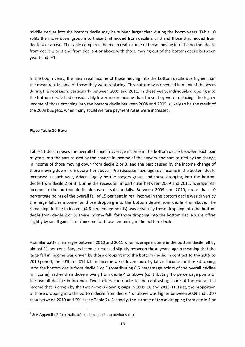
While there were significant changes in mean income and unemployment during the Great Recession in Ireland, the at-risk-of-poverty rate (AROP) did not change as dramatically. Figure 3 shows that the poverty rate, defined as the proportion of persons with income below 60 per cent of median income in each year, fell in the pre-recession period between 2004 and 2007. In the early years of recession, the poverty rate continued to decrease, falling from 16.5 per cent in 2007 to 14.1 per cent in 2009. Between 2009 and 2012 the poverty rate increased, peaking at 16.5 per cent in 2012. In 2013 it fell back to 15.2 per cent.
Under the standard AROP measure, the poverty line is recalculated in each year as 60 per cent of median income. Therefore, while incomes may be falling, the change in the poverty rate will depend on relative income changes at different points along the income distribution. For example, if income decreases are concentrated among persons above the poverty line, then the rate of poverty is likely to decrease despite the overall fall in income. Figure 3 also shows the rate of poverty when the poverty line is calculated as 60 per cent of median income in a base year and adjusted only for inflation. By “anchoring” the poverty line in 2004, when mean real income was close to 2011 levels, the rate of poverty decreased significantly more by 2008 than the standard measure. This is a result of the poverty line being fixed in a period when incomes were lower. As mean income continued to increase during the boom period, and remained higher than the base period in the early years of the recession, the poverty rate remained lower with the fixed poverty line compared to the standard AROP rate. In later years of the recession, when mean income was equal to or below 2004 income, the poverty rate increased significantly more with the fixed poverty line.
Place Figure 3 Here
3. The Evolution of Income Inequality, 2005 to 2013
Given the scale of the macroeconomic changes just described, summary measures of income inequality for Ireland remained remarkably stable over the period. Figure 3shows the Gini coefficient for equivalised household disposable income among persons for the years 2005 to 2013, calculated from the SILC microdata. Household income is equivalised using a scale of 1 for the first adult, 0.66 for additional adults (aged 14 or over) and 0.33 for each child (aged under 14), the scale used in the
6
official measure of poverty in Ireland which is close to that implied by the structure of social welfare payments3
.
Place Figure 4 Here
Figure 4 shows that in 2007, as the economic boom peaked, the Gini coefficient was about 0.31, and remained at about that level between then and 2013 apart from 2009, when it fell temporarily to 0.29 – the only statistically significant difference from one year to the next seen over the period. This reflects the fact that 2009 was when the impact of a series of policy measures had a considerable impact, notably substantial structural innovations and increases in income-related taxes which were progressive, a rise in social welfare payment rates, and progressively structured public service pay cuts (see Callan et al., 2014 for a detailed description and analysis).
It is noteworthy that this stability in the Gini coefficient for Ireland is not limited to the 2004 to 2013 period. Table 1 compares the Gini coefficients for 2004 to 2013 with comparable estimates for 1993, 1994 and 2000, based on the Living in Ireland Survey and the European Community Household Panel (ECHP). We see that this summary measure showed little change, which also appears to be true back to at least 1987 and perhaps 1980 (see Nolan et al, 2012, 2014).
Place Table 1 Here
Examining shares of total disposable income in each decile can highlight changes in the distribution of income which are not evident from summary measures of inequality such as the Gini coefficient. The decile shares in Table 2 reveal that there were significant changes in the share of income going to each decile throughout the recessionary period. Between 2008 and 2009, the only decile that suffered a fall in its share of income was the top decile. Callan et al. (2013) showed that the first austerity budgets contributed to this pattern, when effective tax rates were increased at the same time as an increase in many social welfare rates. This resulted in the richest households losing out the most, at least partly explaining the significantly lower Gini coefficient in 2009.
Between 2009 and 2010, the pattern of decile share changes is almost precisely the reverse of that between 2008 and 2009. In this period, the top decile experienced a significant increase in their share of income, rising above the share it had in 2008. Most other deciles saw a fall in their share of
3 Use of an alternative scale such as the square root of household size or the so-called ‘modified OECD’ scale instead would not affect the pattern over time
7
income. This is particularly true for the bottom decile, whose share fell from 3.6 per cent to 3.1 per cent. Between 2010 and 2013 the decile shares remained reasonably stable. Most changes occurred between the top deciles, where, for example, between 2010 and 2011 the top decile lost 0.7 percentage points in its share of income, but the ninth decile gained 0.4 percentage points.
Place Table 2 Here
Over the entire recessionary period, the largest losses were in the bottom decile; a loss of 0.4 percentage points between 2008 and 2013. The top decile’s share of income remained stable, but the ninth decile’s share increased by 0.5 percentage points. The 2008 decile shares are quite similar to the decile shares from the mid-1990s, as reported by Nolan and Maitre (2000), particularly at the extremes of the income distribution. The second to the sixth deciles have a slightly higher share of income in 2008 than the mid-1990s at the expense of the seventh to ninth deciles.
It must be remembered of course that each decile does not represent the same groups of individuals across years. Rather it measures the share of income going to the poorest 10 per cent of individuals, the second poorest ten per cent of individuals, and so on, in each year. These may not be the same individuals across the years. Section 5 of this paper uses available data to examine the mobility of those in each decile, focusing particularly on those at the bottom of the income distribution. The analysis undertaken here relates to how incomes have changed for the decile groupings – this is the main focus of international work on this topic.
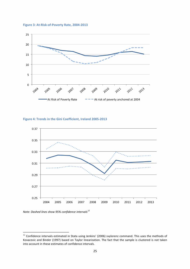
A focus on income shares does not tell the full story of what is happening over this period. As indicated earlier, average incomes are falling, so those income positions which see a fall in income share are also affected by shrinkage in the size of the cake. The net outcomes are reported in Table 3, in the form of percentage losses in income at each decile level. Most commonly, analysis is undertaken in terms of disposable income, without any adjustment for housing costs (i.e., before housing costs). In the UK, analysis is often undertaken at both before housing cost (BHC) and after housing cost (AHC) levels (e.g., Belfield et al., 2014). The arguments for and against each measure may be summarised as follows. Adjustment for housing costs – i.e., spending on housing – is not appropriate if the size of housing costs reflects the preferences of the household for larger or higher quality housing: in these circumstances it would simply reflect a choice of how the household allocates its resources. However, the nature of housing purchases means that individuals may not be free to adjust their housing spending to their current income situation – a high mortgage may be a legacy of earlier decisions. This is particularly relevant to the situation in which a housing bubble burst, leaving many households with high mortgages, while incomes came under pressure via unemployment, lower wages and higher taxes. We find, however, that income distribution analyses over this period are very similar whether conducted on a BHC or AHC basis. Table 3 illustrates this
8
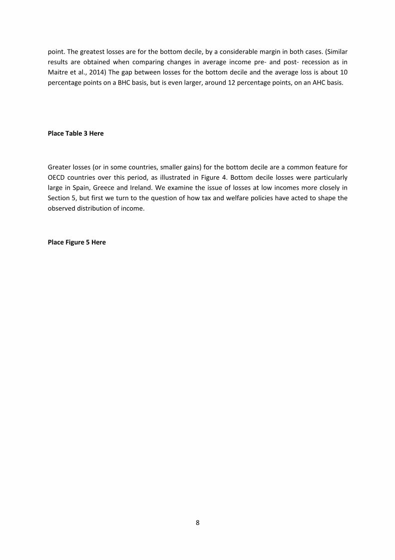
point. The greatest losses are for the bottom decile, by a considerable margin in both cases. (Similar results are obtained when comparing changes in average income pre- and post- recession as in Maitre et al., 2014) The gap between losses for the bottom decile and the average loss is about 10 percentage points on a BHC basis, but is even larger, around 12 percentage points, on an AHC basis.
Place Table 3 Here
Greater losses (or in some countries, smaller gains) for the bottom decile are a common feature for OECD countries over this period, as illustrated in Figure 4. Bottom decile losses were particularly large in Spain, Greece and Ireland. We examine the issue of losses at low incomes more closely in Section 5, but first we turn to the question of how tax and welfare policies have acted to shape the observed distribution of income.
Place Figure 5 Here
9
4. The Role of Tax and Welfare Policies
FitzGerald (2014) stresses that the role of tax and welfare policies in shaping distributional outcomes can be thought of as having two components:
• an impact from discretionary changes in tax and welfare policy, • an “automatic stabilization” component arising from the interaction of macroeconomic
developments and the progressive structure of existing tax and welfare policy
Place Figure 6 Here
The impact of discretionary policy changes can best be measured by examining the impact of such changes on a fixed population. Figure 6 illustrates one such analysis, using the SWITCH model, covering the impact of policy changes introduced between 2009 and 2015 inclusive.4
The pattern is a complex one, which cannot be neatly summarized as progressive, regressive or proportional. Discretionary policy changes had a negative impact across all income deciles. The most negative impact was on the highest income decile (a loss of over 15 per cent), with the next highest impact on the bottom income decile (a loss of over 12 per cent). Most other income deciles saw a loss of between 10 and 11 per cent, with a small loss of 8 per cent for the third income decile.
Turning now to the automatic stabilisation component, this arises because any progressive tax-transfer system does more redistribution when faced with a more unequal income distribution. For example, as unemployment rises, the distribution of market income becomes more unequal. However, if those who are unemployed are entitled to claim income supports, the tax-transfer system will be seen to effect a greater reduction in inequality than before.
The combined impacts of discretionary and automatic elements of the tax and transfer system are summarised in Table 4, which shows Gini and Theil coefficients for market income, gross income (i.e., market income plus transfers) and disposable income (gross income less income-related taxes and employee social insurance contributions). Market income inequality rose sharply between 2008 and 2013. There was a smaller rise in gross income, as social welfare transfers played an equalizing
4 Budgets 2009 to 2015 were a series of “austerity budgets” designed to bring the government deficit and debt under control. The counterfactual used in this analysis is indexation of tax and welfare policy in line with growth in wages, the largest component of national income. The rationale for this approach is set out in a series of papers (Callan et al., 2006; Bargain and Callan, 2010). Analysis based on a counterfactual with tax and welfare parameters frozen in nominal terms would yield very similar results, given that average wages declined by about half of one per cent.
10
role. Direct taxes were also progressive,5
so that both the Gini and the Theil index for disposable income in 2013 are close to their 2008 levels.
Place Table 4 Here
Table 5 examines the redistributive impacts of the transfer system, the direct tax system, and the combination of the two. The measure used is the Reynolds-Smolensky index, which looks simply at the extent to which the Gini coefficient before the policy intervention is reduced by the policy intervention. In the pre-crisis years, the transfer system tended to reduce the Gini coefficient by about 0.15, with the tax system contributing a reduction of a further 0.05. By 2010, the reduction arising from the transfer system had risen to 0.20, remaining at that level through to 2013. There was a more limited rise in the impact of the tax system, from 0.05 to 0.07. Overall, the relative importance of the tax and welfare systems in reducing inequality remained roughly constant: about three quarters of the total reduction coming from the transfer system, and one-quarter from the direct tax system.
Place Table 5 Here
5. Why Have Average Incomes for the Bottom Decile Fallen?
We saw in section 3 that the average income of the bottom decile fell sharply in Ireland over the period 2008 to 2013; and that there were similar sharp falls in a Spain and Greece. Here we focus on the evolution of incomes for the bottom decile from a number of perspectives.
First, we make use of the rotating panel design of the SILC to follow a subset of households, from one year to the next. The broad design is such that 75 per cent of households are eligible for re-interview in the next year. However, sample attrition means that the achieved rate of follow up from one year to the next is closer to 50 per cent. Given this, we look only at households in wave t and wave t+1. Watson (2003) and Nolan et al. (2002) found that while there was substantial attrition in the ECHP and Living in Ireland Surveys, this did not appear to be systematic. Appendix Table B again finds no evidence of systematic attrition bias in the SILC panel, at least along the observable characteristics examined (including age, gender, marital status, labour force status, and income in the top and bottom deciles, among others).
5 Indirect taxes are known to be regressive: for further analysis of indirect taxes see Savage and Callan (2015) and Collins (2014).
11
Figure 7 shows the average income growth for individuals ranked by initial year decile. This is what Bourguignon (2011) called a non-anonymous Growth Incidence Curve, or what Jenkins and Van Kerm (2011) called a mobility profile. Based on the cross-sectional (or anonymous) results, the largest decline in average income between 2008 and 2013 occurred in the bottom decile. By contrast, Figure 5 shows that in each year between 2004 and 2012, the individuals that started in the bottom decile experienced the largest percentage increase in income by the following year. This suggests that there was significant reranking of individuals throughout the income distribution in both boom and recession periods in Ireland. The individuals that started out in the poorest 10 per cent of the population in any given year were not necessarily the same individuals in the poorest 10 per cent the following year.
Place Figure 7 Here
To examine the extent to which individuals moved between deciles, Table 66 examines where individuals in the bottom decile in year t end up in the income distribution in year t+1, for each pair of years between 2004 and 2013. In the pre-crisis years, with the exception of the 2004 to 2005 transitions, close to 9 out of 10 of those in the bottom decile were found in one of the bottom 3 deciles in the next year. This figure fell somewhat during the crisis years, to a level of about 8 out of 10 in 2013. Close to 55 per cent of bottom decile individuals remained in the bottom decile in the pre-crisis years; this figure fell to just under 45 per cent by 20137
.
Place Table 6 Here
Table 7 looks at the converse of this issue: for persons who are in the bottom decile in year t, which decile did they come from in year t-1? Again, with the exception of 2004 to 2005, about 90 per cent of those in the bottom income decile came from one of the bottom three deciles in the pre-crisis years. This figure fell to below 70 per cent in 2010, and by 2013 was at 80 per cent. Looking at longer range mobility, in the immediate pre-crisis years less than 10 per cent of bottom decile individuals came from the top 6 deciles. This figure rose to over 25 per cent in 2010, and fell back to below 10 per cent in 2013.
6 Tables 6 and 7 are weighted by the base year weight. Analysis based on reform year weights produced very similar results. 7 To ensure consistency with the results based on the cross-sectional data, decile cut-offs are calculated using the cross-sectional data. Therefore, when using only the longitudinal observations, each decile may not contain exactly ten per cent of the population. For this reason, the proportion of “stayers” in the bottom decile differs between Tables 6 and Table 7, as Table 6 is based on year 1 decile cut-offs, and Table 7 is based on year 2 decile cut-offs. Jenkins and Van Kerm (2014) follow a similar approach when measuring poverty rates in EU-SILC.
12
Place Table 7 Here
The broad picture painted here is one with considerable stability in the bottom decile from year to year, combined with substantial short-range mobility within the bottom 3 deciles. Downward mobility from the upper part of the income distribution did rise during the worst of the recession, but the composition of the low income deciles remains dominated by those who are in the bottom three deciles from year to year.
We pursue this analysis further by defining 5 different groups which play a role in the composition of the bottom decile in each year (Table 8). The “move out” and “move in” groups arise from the design of the sample (rotating panel) and sample attrition. Here we focus on those who stay in the bottom decile in years t and t+1, those who move up to a higher decile in t+1, or who move down from a higher decile into the bottom decile at time t+1.
Place Table 8 Here
We can gain some insight from Tables 9 to 11 into the issue of whether falls in bottom decile income arise from falls in the income of those who remain at such low income levels, or whether falls in bottom decile income reflect changes in the composition of the decile. Table 98
shows that the largest percentage changes in income are among those who moved between deciles. During the recessionary years, the falls in real income for those dropping into the bottom decile were significantly larger than in previous years, particularly between 2009 and 2011. For those who are “stayers” in the bottom decile, average incomes are either constant or increase slightly. The sharp falls in bottom decile income must then arise from shifts in composition, due to movements in and out of the bottom decile.
Place Table 9 Here
The large decrease in mean real income in the bottom decile (see Table 3) seems therefore to be driven by a reduction of the income of those dropping into the bottom decile, rather than a reduction in the incomes of those already in the bottom decile. The relatively large percentage falls in income for those moving into the bottom decile can be driven by a number of factors. Individuals moving into the bottom decile may have come from positions higher in the income distribution during the recession (which did occur to a certain degree based on Table 7), resulting in larger percentage changes in income. In addition, the falls in real income for those moving from the lower 8 Tables 9 and 10 are weighted by the weight for each individual year. Results were qualitatively equivalent when we used only year t weights, and only year t+1 weights. Results available upon request.
13
middle deciles into the bottom decile may have been larger than during the boom years. Table 10 splits the move down group into those that moved from decile 2 or 3 and those that moved from decile 4 or above. The table compares the mean real income of those moving into the bottom decile from decile 2 or 3 and from decile 4 or above with those moving out of the bottom decile between year t and t+1.
In the boom years, the mean real income of those moving into the bottom decile was higher than the mean real income of those they were replacing. This pattern was reversed in many of the years during the recession, particularly between 2009 and 2011. In these years, individuals dropping into the bottom decile had considerably lower mean income than those they were replacing. The higher income of those dropping into the bottom decile between 2008 and 2009 is likely to be the result of the 2009 budgets, when many social welfare payment rates were increased.
Place Table 10 Here
Table 11 decomposes the overall change in average income in the bottom decile between each pair of years into the part caused by the change in income of the stayers, the part caused by the change in income of those moving down from decile 2 or 3, and the part caused by the income change of those moving down from decile 4 or above9
. Pre-recession, average real income in the bottom decile increased in each year, driven largely by the stayers group and those dropping into the bottom decile from decile 2 or 3. During the recession, in particular between 2009 and 2011, average real income in the bottom decile decreased substantially. Between 2009 and 2010, more than 10 percentage points of the overall fall of 15 per cent in real income in the bottom decile was driven by the large falls in income for those dropping into the bottom decile from decile 4 or above. The remaining decline in income (4.8 percentage points) was driven by those dropping into the bottom decile from decile 2 or 3. These income falls for those dropping into the bottom decile were offset slightly by small gains in real income for those remaining in the bottom decile.
A similar pattern emerges between 2010 and 2011 when average income in the bottom decile fell by almost 11 per cent. Stayers income increased slightly between these years, again meaning that the large fall in income was driven by those dropping into the bottom decile. In contrast to the 2009 to 2010 period, the 2010 to 2011 falls in income were driven more by falls in income for those dropping in to the bottom decile from decile 2 or 3 (contributing 8.5 percentage points of the overall decline in income), rather than those moving from decile 4 or above (contributing 4.6 percentage points of the overall decline in income). Two factors contribute to the contrasting share of the overall fall income that is driven by the two movers down groups in 2009-10 and 2010-11. First, the proportion of those dropping into the bottom decile from decile 4 or above was higher between 2009 and 2010 than between 2010 and 2011 (see Table 7). Secondly, the income of those dropping from decile 4 or
9 See Appendix 2 for details of the decomposition methods used.
14
above was almost 30 per cent lower than the movers up group in 2009-10, while it was just above 20 per cent lower than the movers up group in 2010-11.
Place Table 11 Here
Employment loss was a significant contributory factor in the large contribution of those moving from decile 4 or above to the overall fall in bottom decile income between 2009 and 2010. As income is measured over the 12 months prior to interview in SILC10
6. Conclusions and Further Research
, the 2009 to 2010 income changes cover the period during which unemployment in Ireland increased from about 6 per cent in 2008 to over 14 per cent during 2010. Between 2009 and 2010, more than 1 in 4 of those that dropped into the bottom decile from decile 4 or above lived in a household where someone became unemployed, while just under half of the individuals falling into the bottom decile from decile 4 or above lived in a household that had one less person in employment in 2010 than in 2009. Reduced numbers of individuals in employment in a household can arise from migration, retirement or individuals exiting the labour market, as well as the effect of unemployment.
After an unprecedented economic boom peaking in 2007, Ireland was one of the countries worst affected by the onset of the Great Recession, and faced a remarkably challenging fiscal adjustment in the context of a ‘bail-out’ by the EU and IMF. By 2014 Ireland had successfully completed a stringent bail-out programme, economic growth had returned, and unemployment was falling rapidly. The scale and nature of its Great Recession makes Ireland a particularly interesting case-study, and the fact that it has been hailed in some circles as an exemplar for embracing austerity makes a comprehensive assessment of the distributional consequences all the more important.
Despite extraordinary changes at the macroeconomic level, we have seen that summary measures of income inequality remained quite stable throughout the adjustment period. However, more detailed analysis of incomes at different points in the income distribution shows that there were some changes in the income distribution which are not captured by such summary measures. Over the entire recessionary period from 2008 to 2013, the bottom decile’s share in total disposable income fell by 0.4 percentage points, with its real income falling by 22 per cent compared with the average loss across the entire distribution of 13 per cent. Examination of income after housing costs produced broadly similar results, with the lowest decile experiencing the largest decline in income through the recession.
These results are based on “snapshots” or cross-sections of the income distribution in a given year. Thus, the individuals making up a particular income group vary over time. The rotating panel component of the survey allowed us to examine transitions between deciles and the changes in real
10 So, for example, the income data for a household in SILC 2009 interviewed in June 2009 would cover the period June 2008 to June 2009.
15
income for those remaining in versus moving to a particular decile from one year to the next. We found that about half of the bottom decile in each year remained in the lowest decile in the following year, those who entered the bottom decile came mainly from the second and third deciles, but there was an increase in longer range downward mobility into the bottom decile during the years of deepest recession. Using a decomposition method developed for the purpose, we showed that the large decline in average income for the bottom decile between 2009 and 2010, at the onset of the Crisis, was driven by those falling from the middle and upper part of the income distribution, in part due to loss of employment. Between 2010 and 2011, however, when average income again fell significantly, it was individuals falling from the 2nd and 3rd deciles caused the majority of that decline. This longitudinal perspective provides an important complement to the more commonly reported cross-sectional results, which find the greatest income losses concentrated at the lowest income positions. It is clear from the longitudinal perspective that this does not imply that the greatest income losses were felt by those who were at the bottom of the distribution as the Crisis struck.
What role did redistribution play? The progressive structure of the Irish tax/transfer system meant that, with the advent of the recession it automatically worked harder than before the recession to offset the increased inequality associated with greater unemployment and sharp falls in income. This could be termed the “automatic stabilisation” component of policy. As far as choices about redistributive parameters are concerned, the series of “austerity budgets” implemented to deal with soaring government deficit and debt had distributional impacts which varied a good deal from one budget to another, and also depended on which measures were incorporated into the distributional analysis. Discretionary changes in policy (i.e., changes compared with a neutral budget) gave rise to complex effects. Over the entire period of adjustment, and including not only changes in income tax and cash transfers but also public sector pay cuts, increases in indirect taxes and new property taxes, we saw that the most negative impact was on the highest income decile with a loss of over 15 per cent, while most other income deciles saw a loss of 10-11 per cent and the bottom decile lost 12 per cent. The combined impacts of discretionary and automatic elements of the tax and transfer system were to reduce the Gini coefficient going from market to disposable income by about 0.27 by 2013, up from 0.20 before the onset of the Crisis, with about three quarters of the total reduction coming from the transfer system and one-quarter from the direct tax system.
One’s view of the Ireland’s successful fiscal adjustment from a distributional perspective, in light of this evidence, will then be a matter of both judgement and preferences: the relatively large income losses seen at the bottom of the distribution need to be interpreted with care, but leaving that aside, how one views a broadly proportional sharing of the income losses associated with severe recession will depend on both one’s distributional preferences and one’s view of the feasible alternatives. From a methodological and analytical point of view, the paper brings out the importance of going beyond comparison of cross-sectional income shares over time to incorporate a longitudinal perspective, of broadening the focus in assessing policy impacts beyond the realm of income tax and cash transfers for which microsimulation approaches to distributional assessment were initially developed (as other more recent studies such as Avram et al, 2014 have sought to do), and of setting the results of analysis of discretionary policy impacts in the broader context of the role of automatic stabilisers and overall distributional change.
16
Appendix A: Data
The main source of data used in the analysis is the Irish Survey of Income and Living Conditions (SILC). The survey has been conducted by the Central Statistics Office (CSO) of Ireland every year since 2003 and contains a range of microdata on income, poverty, social exclusion and living conditions. In the first survey year, 2003, only six months of data was collected, and the sample size was approximately half of the other survey years. We therefore omit this wave from our analysis. Each of the 2004 to 2013 contains more than 11,000 individuals, or more than 4,000 households. We are primarily concerned with the distribution of equivalised household disposable income, although we also examine changes in the distribution of market income and gross income. For each of the income types we equivalise using a scale of 1 for the first adult, 0.66 for subsequent adults, and 0.33 for children (aged 14 or less)11
. Section 4 and 5 rely largely on cross-sectional SILC surveys from 2004 to 2013. In section 6, we also make use of the panel element of SILC.
SILC Longitudinal 2004 to 2013
To investigate patterns observed in the cross-sectional analysis, it is useful to be able to track individuals and households from one period to the next. The longitudinal element of SILC is designed so that 75 per cent of households in a given year are sought for interview in the following year. However, a significant rate of sample attrition means that the retention rate of households is closer to 50 per cent in each year, as can be seen in Table 1. This significant rate of household attrition raises the possibility of selection biases being introduced when using the longitudinal data. These biases may occur if attrition is related to characteristics of the household such as income, marital status, poverty status, household composition and so on. To check whether such biases exist in the longitudinal element of each year’s SILC, Appendix Table B compares a number of key characteristics of individuals in the cross-section and panel elements of each year of SILC used in this analysis.
11 This is the equivalence scale used by the CSO in calculating poverty and income distribution statistics, and closely matches that implied by the rates of the main social welfare payments in Ireland.
17
Place Appendix Table A Here
The results suggest that the degree of bias introduced by sample attrition is quite limited. For the majority of cases, the distribution of variables (percentages or € values) from the longitudinal data represent between 90 per cent and 110 per cent of the cross-section value. For example, 19.5 per cent of individuals live in 2-person households in the 2005 wave of SILC. Of the observations in the 2005 wave who are also present in the 2006 wave of SILC, 19.6 per cent live in two-person households. Similarly, 72.8 per cent of individuals live in households with 3 or more people according to the 2005 cross-section, compared to 72.3 per cent of the longitudinal respondents. While one might expect that low income households may be under-represented in longitudinal surveys, the evidence in Appendix Table B suggests this is not evident in the longitudinal element of SILC. The mean income in the bottom decile is within 3 per cent of the cross-sectional value in all eight years of comparison. Similarly, the poverty rate among the longitudinal respondents is within 1 percentage point of the poverty rate in the full cross-section in five of the eight years of comparison; the difference in poverty rates is above 2 percentage points in just one of the eight years (2005).
There are some comparisons that indicate that attrition may be non-random by certain characteristics. For example, a lower proportion of individuals among the longitudinal respondents live in households where the head is aged less than 30 compared to the full cross-sections, particularly before 2010. Conversely, a higher proportion of individuals live in households with a head aged 65 or older, or where the household head is retired, among the longitudinal respondents than the full cross-section. The most consistent pattern emerges in the comparison of urban and rural respondents. The proportion of rural respondents among the longitudinal observations is more than ten per cent higher than the cross-sectional observations in six of the eight years of analysis. These patterns are consistent with Nolan et al.’s (2002) results based on the longitudinal element of the Living in Ireland Survey where attrition was also greater for urban households. They also suggested that attrition is most likely among those with the highest propensity to change address, such as young adults.
Overall, the evidence suggests that, despite the relatively high rate of attrition, the year-to-year changes for the panel respondents are broadly representative of changes for the full population. While the pattern of attrition was not always random, the impact on the structure of the sample over two waves was modest.
Place Appendix Table B Here
19
Appendix B: Decomposition Methods
In this appendix section, we briefly summarise the decomposition methods used in Section 5. A forthcoming ESRI working paper by Savage (2015) provides greater detail on the decomposition approach. The decomposition proceeds as follows: Year t average income in the bottom decile can be written as:
𝜇𝑡1 = 𝜎𝑠𝜇𝑡𝑠 + (1 − 𝜎𝑠)𝜇𝑡𝑚𝑢 (1)
where 𝜇𝑡1 t is average income in decile 1 at year t, 𝜎𝑠 is the share of the bottom decile occupied by stayers, 𝜇𝑡𝑠 t is the average income of the stayers in year t, and 𝜇𝑡𝑚𝑢 is the average income of movers up in year t.
Similarly, we can write average income in the bottom decile in year t + 1 as:
𝜇𝑡+11 = 𝜎𝑠𝜇𝑡+1𝑠 + (1 − 𝜎𝑠)𝜇𝑡+1𝑚𝑑 (2)
where 𝜇𝑡+1𝑚𝑢 is the average income of the movers down group in year t + 1.
Using equations 1 and 2, we can write the change in average income in the bottom decile between year t and year t + 1 as:
𝛿1 = 𝜇𝑡+11 𝜇𝑡1 − 1⁄ (3)
By defining two counterfactual income scenarios, we can isolate the impact of the changes in income of the various groups identified in Table 1. CF1 is the distribution of income if the income of the “stayers” group in year t + 1 is held constant at its year t value, and all other incomes are allowed to change. Average income in the bottom decile in this first counterfactual income scenario can be calculated as:
20
𝜇𝑐𝑓11 = 𝜎𝑠𝜇𝑡𝑠 + (1 − 𝜎𝑠)𝜇𝑡+1𝑚𝑑 (4)
The “movers effect”, or the change in average income in the bottom decile if only the income of those transitioning into and out of the bottom decile changed, can therefore be calculated as:
𝛿𝑐𝑓11 = 𝜇𝑐𝑓11 𝜇𝑡1 − 1⁄ (5)
Conversely, the second counterfactual income distribution, CF2, is the distribution of income when only the income of the stayers is allowed to change to its year t+1 value. All other incomes are held at their year t values. In this case, average income in the bottom decile can be calculated as:
𝜇𝑐𝑓21 = 𝜎𝑠𝜇𝑡+1𝑠 + (1 − 𝜎𝑠)𝜇𝑡𝑚𝑢 (6)
The “stayers effect” can therefore be calculated as:
𝛿𝑐𝑓21 = 𝜇𝑐𝑓21 𝜇𝑡1 − 1⁄ (7)
The proportion of the overall change in income that can be attributed to the “stayers effect” and the “movers effect” is straightforward to calculate, based on the fact that:
𝛿1 = 𝛿𝑐𝑓11 + 𝛿𝑐𝑓21 (8)
In section 5, the decomposition is simply extended to isolate the impact of those that drop into the bottom decile from deciles 2 or 3, and those that drop into the bottom decile from decile 4 or above using a similar logic.
21
References
Agnello, L. and R.M. Sousa, "How Does Fiscal Consolidation Impact on Income Inequality?," Review of Income and Wealth, 60 (4), 702-726, 2014
Belfield, C., J. Cribb, A. Hood, R. Joyce, Living Standards, Poverty and Inequality in the UK: 2014, Institute for Fiscal Studies, London, 2014.
Bourguignon, F., “Non-anonymous growth incidence curves, income mobility and social welfare dominance”, Journal of Economic Inequality, 9(4), 605-627, 2011.
Kovaevic, M.S. and D.A. Binder, “Variance estimation for measures of income inequality and polarization” Journal of Official Statistics, 13(1), 41-58, 1997.
Callan T., C. Leventi, H. Levy, M. Matsaganis, A. Paulus and H. Sutherland, “The distributional effects of austerity measures: a comparison of six EU countries” Research Note 2/2011 of the European Observatory on the Social Situation and Demography, European Commission, 2011.
Callan, T., Nolan, B., Keane, C., Savage, M., Walsh, J.R., "Crisis, Response and Distributional Impact: the Case of Ireland", IZA Journal of European Labor Studies, 3 (9), http://www.izajoels.com/content/3/1/9, 2014.
Collins, M., Total Direct and Indirect Tax Contributions of Households in Ireland: Estimates and Policy Simulations, Working Paper 18, Nevin Economic Research Institute, Dublin, 2014.
FitzGerald, J., “The Distribution of Income, Social Welfare and the Public Finances”, Quarterly Economic Commentary, Summer, Economic and Social Research Institute, Dublin, 2014.
Keane, C., Callan, T., Savage, M., Walsh, J. R, Colgan, B., "Distributional Impact of Tax, Welfare and Public Service Pay Policies: Budget 2015 and Budgets 2009-2015", Quarterly Economic Commentary, Winter, Economic and Social Research Institute, Dublin, 2014.
Herault, N. and F. Azpitarte, “Understanding Changes in the Distribution and Redistribution of Income: A Unifying Decomposition Framework”, Review of Income and Wealth, DOI: 10.1111/roiw.12160, 2014.
Jenkins, S. P., svylorenz: Stata module to derive distribution-free variance estimates from complex survey data, of quantile group shares of a total, cumulative quantile group shares, SSC Archive S456602, http://ideas.repec.org/c/boc/bocode/s456602.html., 2006.
Jenkins, S. and P. V. Kerm, “The Relationship Between EU Indicators of Persistent and Current Poverty”, Social Indicators Research 116 (2), 611-638, 2014.
Jenkins, S. P. and P. Van Kerm, Trends in Individual Income Growth: Measurement Methods and British Evidence. IZA Discussion Papers 5510, Bonn: Institute for the Study of Labor (IZA), 2011.
Maitre, B., H. Russell and C.T. Whelan, “Trends in Economic Stress and the Great Recession in Ireland: An Analysis of the CSO Survey on Income and Living Conditions (SILC)”, Dublin: Department of Social Protection, Social Inclusion Technical Paper No. 5, 2014.
Madden, D., “Health and Wealth on the Roller-Coaster: Ireland, 2003–2011” Social Indicators Research , 387-412, 2014a.
Madden, D. “Winners and Losers on the Roller-Coaster: Ireland, 2003-2011” The Economic and Social Review, 45(3), 405-421, 2014b.
Matsaganis, M. The Greek Crisis: Social Impact and Policy Responses, Friedrich Ebert Stiftung, Berlin, 2013.
Matsaganis, M. and C. Leventi, “Inequality, poverty and the crisis in Greece”, ETUI Policy Brief, European Economic and Employment Policy Issue 5/2011.
Nolan, B., B. Gannon, R. Layte, D. Watson, C.T. Whelan, J. Williams, Monitoring Poverty Trends in Ireland: Results from the 2000 Living in Ireland Survey, Policy Research Series 45, Economic and Social Research Institute, Dublin, 2001.
Nolan, B., B. Maitre, S. Voitchovsky and C.T. Whelan, Inequality and Poverty in Boom and Bust: Ireland as a Case Study, GINI Discussion Papers 70, AIAS, Amsterdam Institute for Advanced Labour Studies, 2012.
Nolan, B., et al., ‘Ireland: Inequality and Its Impacts in Boom and Bust’, in B. Nolan, W. Salverda, D. Checchi, I. Marx, A. McKnight, I.G. Tóth and H. van de Werfhorst, eds. 2014. Changing Inequalities and Societal Impacts in Rich Countries: Thirty Countries’ Experiences, Oxford University Press, Oxford, 2014
OECD. Society at a Glance 2014, OECD, Paris 2014a.
OECD, “Rising inequality: youth and poor fall further behind”, Income Inequality Update, June, OECD, Paris, 2014b.
Peichl, A., N. Pestel and H. Schneider, "Does Size Matter? The Impact Of Changes In Household Structure On Income Distribution In Germany," Review of Income and Wealth, vol. 58(1), pp. 118-141, 2012.
PRTB, “The PRTB Rent Index Quarter 3 2014” http://www.prtb.ie/docs/default-source/rent-index/prtb-quarter-3-2014-report-v3.pdf?Status=Temp&sfvrsn=2 [accessed 04/03/2015]
Savage (forthcoming) ................
Van Kerm, P. and M. Alperin, Inequality, growth and mobility: the inter-temporal distribution of income in European countries 2003-2007, Publications Office of the European Union, Luxembourg, 2011.
Watson, D., “Sample Attrition between Waves 1 and 5 in the European Community Household Panel”, European Sociological Review, 19 (4), 2003.
Whelan, C.T., and B. Maitre “The Great Recession and the changing distribution of economic vulnerability by social class: The Irish case” Journal of European Social Policy, 24 (5), 470-485, 2014.
24
Figure 1: ILO Unemployment Rate (seasonally-adjusted), Ireland, 1998 to 2013
Figure 2: Average Household Disposable Income per Adult Equivalent, 2004-2013
Source: Author’s analysis of SILC Research Microdata Files.
Notes: 1. Disposable income is before housing costs, and the equivalence scale is that used in the Irish national poverty target (1 for the first adult, 0.66 for subsequent adults, 0.33 for children aged under 14. 2. The adjustment from nominal to real income is calculated by the authors based on the CPI for the relevant year. Results are broadly similar to those reported by CSO in SILC publications, which make a more refined adjustment allowing for the time pattern of data collection.
25
Figure 3: At-Risk-of-Poverty Rate, 2004-2013
Figure 4: Trends in the Gini Coefficient, Ireland 2005-2013
Note: Dashed lines show 95% confidence intervals12
12 Confidence intervals estimated in Stata using Jenkins’ (2006) svylorenz command. This uses the methods of Kovacevic and Binder (1997) based on Taylor linearization. The fact that the sample is clustered is not taken into account in these estimates of confidence intervals.
26
Figure 5: OECD Analysis: Poorer Households Tended to Lose More or Gain Less - Annual percentage changes in household disposable income between 2007 and 2011, by income group
Source: OECD (2014b)
Figure 6: Impact of Budgetary Policy 2009-2015 - Percentage Change in Disposable Income by Income Decile
Source: SWITCH model at December 2014 incorporating main changes in direct tax, welfare and public service
pay/pensions, and water charges; augmented by results on carbon tax and VAT, DIRT, specific Budget 2014 restrictions of tax reliefs for pension contributions and medical insurance premia, and Capital Gains Tax as described in Callan et al. (2013b).
27
Figure 7: Percentage Change in Average Real Income by Base-Year Decile
28
Table 1: Gini Coefficients, Selected Years, 1994 to 2013
Sources: 1994 and 2000 from Living in Ireland Survey as reported by Nolan et al. (2012). All other years from authors’ calculations based on SILC Research Microdata File.
Notes: Gini coefficients calculated from the Household Budget Surveys of 1994/95 and 2000/01 are each 0.30
Table 2: Decile Shares of equivalised disposable income among persons, 1994 to 2013
10 24.4 24.3 24.8 25.6 25.7 24.7 24.4 23.1 24.7 24.0 23.9 24.4 Notes: 1994 and 1997 from Nolan and Maitre (2000). All other years from authors’ calculations based on SILC Research Microdata File.
29
Table 3: Changes in Average Real Incomes by Decile of Equivalised Disposable Income 2008- 2013
% Change from 2008 –2013
Decile Before Housing Costs After Housing Costs Bottom -22.1 -27.2
Appendix Table B: Characteristics of All Individuals at Year t in SILC Cross-Section Year t, and of Individuals at Year t who are in SILC Panel in Year t and Year t+1