75
1 THE HANDBOOK OF FOOD ENGINEERING PRACTICE CRC PRESS CHAPTER 10 KINETICS OF FOOD DETERIORATION AND SHELF-LIFE PREDICTION Petros S. Taoukis, Theodore P. Labuza and Israel Sam Saguy

1
THE HANDBOOK OF
FOOD ENGINEERING PRACTICE
CRC PRESS
CHAPTER 10
K INETICS OF FOOD DETERIORATIONAND
SHELF -LIFE PREDICTION
Petros S. Taoukis, Theodore P. Labuza and Israel Sam Saguy

2
10.1 INTRODUCTION
Quality is an attribute of food, on which understandably a lot of consideration
is focused. Food quality can be defined as the assemblage of properties which
differentiate individual units and influence the degree of acceptability of the food by the
consumer or user (Kramer and Twigg, 1968). Due to the nature of foods as a
physicochemically and biologically active systems, food quality is a dynamic state
continuously moving to reduced levels (with the notable exception of the cases of
maturation and aging). Therefore, for each particular food, there is a finite length of time
after production it will retain a required level of quality organoleptically and safetywise,
under stated conditions of storage. This period of time can be generally defined as the
shelf life of the food product. There is no established, uniformly applicable definition of
shelf life. The definition of shelf life and the criteria for the determination of the end of
shelf life are dependent on specific commodities and on the definition's intended use (i.e.,
for regulatory vs. marketing purposes). Food related authorities have proposed various
definitions that can serve as guidelines. The International Institute of Refrigeration (IIR)
recommendations for frozen food (IIR, 1972) introduce two different definitions. High
Quality Life (HQL) is the time from freezing of the product for a just noticeable sensory
difference to develop (70-80% correct answers in a triangular sensory test). Another type
of shelf life definition that can be extended to other types of food products is the Practical
Storage Life (PSL). PSL is the period of proper (frozen) storage after processing
(freezing) of an initially high quality product during which the organoleptic quality remains
suitable for consumption or for the process intended. PSL is usually in the order of two
to three times longer than HQL. Time of minimum durability, introduced by the EEC
directive on food labeling, and defined as the time during which the foodstuff retains its
specific properties when properly stored is different in principle from the aforementioned
ones, in that it relates to properties of the product itself and not to considerations of its use.

3
It is a working definition for the food scientist satisfying the often made fundamental
assumption that the highest quality product is the freshly processed (or harvested) one.
However, since characteristic properties are overlaid, a decision has to be made at what level
the change in a certain characteristic or the development of an undesirable one can be
detected by the consumer. For example, if having a specific flavor means the absence of
off flavors, it has to be decided at what intensity levels are these flavors detectable by the
consumer. Thus this definition is closely related to the HQL definition.
For any definition to be used as a working tool it has to be followed by further
guidelines i.e. the meaning of organoleptic quality has to be accurately defined and
appropriate methods of measuring it and criteria for setting acceptability limits must be
discussed.
Sensory evaluation by a trained panel, whereby the food is graded on a
"standardized" hedonic scale, usually best approximates the overall quality state of the food
(Labuza and Schmidl, 1988). This approach is not without problems. There are
considerable difficulties in establishing a meaningful scale for each food product. An
expert panel is not necessarily representative of consumers, let alone different consumer
segments (Mackie et al., 1985). Even if that assumption can be made, a cut-off level of
acceptability has to be decided upon. The time at which a large (but preset) percentage of
panelists judge the food as being at or beyond that level is the end of shelf life (PSL). A
criterion like that includes an indication of the proportion of the consumers to which the
product must be acceptable till the end of shelf life, another variable to which reference or
agreement is required. Other problems of the sensory approach are the high cost that is
involved with large testing panels and the questions connected with tasting spoiled or
potentially hazardous samples. In some cases microbial growth or nutrient degradation
could reach unacceptable levels while the food is still judged organoleptically acceptable.
Sensory data are not "objective" enough for regulatory purposes and in cases of legal
4
action or dispute. Sometimes consumers can be "trained" to accept lower standard
products by being exposed to products of gradually slipping quality. That makes the need
of alternative ways of assessing quality apparent (Herborg, 1985).
Chemical, microbiological and physical tests are being used widely in the study
of food quality. Characteristics used by the consumer for evaluation of a product, such as
flavor, color and textural properties can be measured instrumentally or chemically. The
study of the chemical and biological reactions and physical changes that occur in the food
during and after processing allows the recognition of the ones that are most important to its
safety, integrity and overall quality. Physicochemical or microbiological parameters can be
used to quantitatively assess quality. The values of these parameters can be correlated to
sensory results for the same food and a limit that corresponds to the lowest acceptable
organoleptic quality can be set. However, caution should be drawn to the fact that
correlation of values of individual chemical parameters to sensory data is often not
straightforward because overall organoleptic quality is a composite of a number of
changing factors (Trant et al., 1981). The relative contribution of each factor to the overall
quality may vary at different levels of quality or at different storage conditions.
Despite the discussed difficulties in defining and evaluating quality and
determining shelf life of a food, a lot of progress has been made towards a scientific and
generally accepted approach. It is an area of continuous and extensive research. An in-
depth study of the different deteriorative mechanisms that occur in a food system and
systematic analysis and interpretation of the results lead to more meaningful and
objectively measurable ways of assessing food quality and determining shelf life. Proper
application of chemical kinetic principles to food quality loss is essential for efficiently
designing appropriate tests and analyzing the obtained results.

5
10.2 KINETICS OF FOOD DETERIORATION
10.2.1. Reaction modeling principles
Applying fundamental chemical kinetic principles the rate of food quality change may in
general be expressed as a function of composition and environmental factors (Saguy and
Karel, 1980):
dQdt = F (Ci, Ej) (1)
where Ci, are composition factors, such as concentration of reactive compounds, inorganic
catalysts, enzymes, reaction inhibitors, pH, water activity, as well as microbial populations
and Ej environmental factors, such as temperature, relative humidity, total pressure and
partial pressure of different gases, light and mechanical stresses. What the food kineticist
is thus faced with, is a physicochemical system of high complexity involving numerous
physical and chemical variables and coefficients which in most cases are imposible or
impractical to quantitatively define. Even if the system could be explicitly expressed in
terms of measurable parameters, an analytical solution is usually nonexistent and exact
numerical solutions are too complicated and laborious to be useful as working tools.
The established methodology consists of first identifying the chemical and
biological reactions that influence the quality and the safety of the food. Then, through a
careful study of the food components and the process, the reactions judged to have the
most critical impact on the deterioration rate, are deternined (Labuza, 1985). Excluding the
effect of the environmental factors, Ej, by assuming them constant, at the most propable
level or judging it negligible within their expected variation, a simplified reaction scheme
that expresses the effect of the concentration of the reactants, is developed. The ultimate

6
objective is to model the change of the concentrations of constituents connected to food
quality, as functions of time. Molecular, irreversible reactions are typically expressed as
µ1 A1 + µ2 A2 + µ3 A3 + .... + µm Am →kf P (2)
where Ai are the reactant species, µj the respective stoichiometric coefficients (j=1,2...m), P
the products and kf the forward reaction rate constant. For such a scheme the reaction rate,
r, is given (Hills and Grieger-Block, 1980) by:
r = - 1µj
d[Aj]
dt = kf [A1]n1 [A2]
n2 ...... [Am]nm (3)
where nj is the order of the reaction with respect to species Aj. For a true molecular
reaction, it holds that: nj = µj. More often than not, the degradation of important
components to undesirable products is a complex, multistep reaction for which the limiting
reaction and intermediate products are difficult to identify. A lot of reactions are actually
reversible having the form:
α A + β B →←kf
kb
γ C + δ D (4)
In this case A reacts with B to form products C and D which can back react with a rate
constant of kb. The reaction rate in this case would be:
r = -d[A]α dt
= -d[B]β dt
= +d[C]γ dt
= +d[D]δ dt
= kf [A] α [B]β - kb [C]γ [D]δ (5)
For the majority of food degradation systems either kb is negligible compared to kf, or for
the time period of practical interest they are distant from equilibrium, i.e.[C] and [D] are

7
very small, allowing us to treat it as an irreversible reaction. In most cases the
concentration of the reactant that primarily affects overall quality is limiting, the
concentrations of the other species being relatively in large excess so that their change with
time is negligible (Labuza, 1984). That allows the quality loss rate equation to be
expressed in terms of specific reactants, as:
r = -d[Α]
dt = kf' [Α]αααα (6)
where αααα is an apparent or pseudo order of the reaction of compoment A and kf' is the
apparent rate constant. Another case that can lead to a rate equation similar to equation (6)
is when the reactants in reaction (2) are in stoichiometric ratios (Hills, 1977). Then from
equation (3) we have:
r= kf ∏
im [A i]
ni = kf
∏
i
m
µini
A1
n1 ∑ni
(7)
or r = -d[A]
dt = kf' [A]αααα (8)
where A = A1 and αααα = Σni, an overall reaction order.
Based on the aforementioned analysis and recognizing the complexity of food
systems, food degradation and shelf life loss is in practice represented by the loss of
desirable quality factors A (e.g. nutrients, characteristic flavors) or the formation of
undesirable factors B ( e.g. off flavors, discoloration). The rates of loss of A and of
formation of B are expressed as in eq. (6), namely:

8
rA = -d[A]
dt = k [A]m (9)
rB = d[B]dt = k' [B]m' (10)
The quality factors [A] and [B] are usually quantifiable chemical, physical, microbiological
or sensory parameters characteristic of the particular food system. Both k and k' are the
apparent reaction rate constants and m and m' the reaction orders. It should be again
stressed that equations (9) and (10) do not represent true reaction mechanisms and m and
m' are not necessarily true reaction orders with respect to the species A and B but rather
apparent or pseudo orders. The apparent reaction orders and constants are determined by
fitting the change with time of the experimentally measured values of [A] or [B] to
equations (9) or (10). The techniques used for the solution can be generally classified into
two categories: a) Differential Methods and b) Integral Methods (Hills and Grieger-Block,
1980).
In experimental kinetic studies, it is impossible to measure the reaction rate
itself. Instead, the concentration of A or B is measured (directly or indirectly) as a function
of time. If these concentrations are plotted against time and smooth curves are fitted either
graphically or using a statistical fitting method (e.g., polynomial regression) the reaction
rates may be obtained by graphical or numerical differentiation of the curves. By taking
the logarithm of both sides of equation (9) and (10), the following linear expressions are
obtained:
log rA = log k + m log [A] (11)
log rB = log k' + m' log [B] (12)

9
Data can be fitted to these equations by the method of least squares to determine values of
the constants.
Two differential approaches can be alternatively used. The first involves
differentiation of data obtained from a single experimental run. It requires measurement of
A or B concentrations with time, to at least 50% conversion. The second is differentiation
of data from initial rate measurements. In this approach, measurements of concentrations
are carried out to very small conversions (e.g., 5%). This is repeated for a number of initial
reactant concentrations. Thus, each estimated rate corresponds to a different initial reactant
concentration and involves a separate experimental run. Another difficulty often faced with
this method is in fitting data from kinetic experiments in which the rate changes rapidly
even within the low conversions that are used (e.g., in case of enzymatic reactions). One
has to obtain an initial slope from a set of data points with a rapid change in slope and also
inevitable scatter from experimental errors. The usual methods of least square fitting of a
polynomial may give erratic estimates of the initial slope. A flexible mathematical method
to overcome this problem is the use of spline functions (Wold, 1971). The major
advantage of the spline function method is that it uses all the data to estimate the intial rate,
but is not unduly influenced by experimental error in individual data points.In general, the
differential methods involve two statistical fittings, thus being more sensitive to
experimental scattering and requiring a large number of data points for a dependable
parameter estimate.
In the integral method, variables in equations (9) and (10) are separated and
integration is carried out. For example for equation (9), we have:
- ⌡⌠
Ao
A
d[A]
[A] m = k t (13)

1 0
Regardless of the value of m, equation (13) can be expressed in the form:
Q(A) = k t (14)
where the expression Q(A) is defined as the quality function of the food.
The form of the quality function of the food for an apparent zero, 1st, 2nd and
mth order reaction can be derived from the eq.(14) and is shown in the following Table 1.
The half life time of the reaction i.e. the time for the concentration of the quality index A to
reduce to half its inital value is also included.
Table 1. Quality function form and half life times for different order reactions.
Apparent Reaction Quality Function Half Life timeOrder Q(A)t t1/2
0 Ao - At Ao/(2ko)
1 ln ( Ao/At) ln2/k1
2 1/Ao-1/At 1/(k2Ao)
m(m≠1)1
m-1 (A1-mt -A
1-mo )
2m-1-1km(m-1) A
1-mo
To determine the quality function one assumes different values of m (0, 1 or
other) and tries out a graphical or a least square linear fit to the corresponding equations
(Table 1) of the experimental data. If the experiment has been carried out to at least 50%
conversion and preferably 75%, it is usually easy to determine which reaction order and
equation gives the best fit, either graphically or by using statistical goodness of fit criteria.
The coefficient of determination (R2) of the linear regression is in most cases a sufficient

1 1
criterion. The value of the R2, for a least square fit in general, is given by the following
equation:
R2 = 1 -
∑
i=1
N
(yi - yi)2/∑i=1
N
(yi - y_)2 (15)
where yi the experimentally observed values of the measured parameter (i=1 to
N), y i the value predicted from the regression equation, y_ the average of the observed
values and N the number of measurements (Ott, 1984). The correct apparent order is that
for which the R2 is closer to unity. The overwhelming majority of the food reactions that
have been studied have been characterized as pseudo-zero or pseudo-first order (Labuza,
1984). Characteristic examples are listed in Table 2.
Table 2.Important quality loss reactions that follow zero or first order kinetics.
Zero order • Overall quality of frozen foods
• Non-enzymatic browning
First order • Vitamin loss
• Microbial death / growth
• Oxidative color loss
• Texture loss in heat processing
Caution is advised in deciding the appropriate apparent order and quality
function, as noted by Labuza (1988). For example when the reaction is not carried far
enough (less than 50% conversion) both zero and first order might be indistinguishable
from a goodness of fit point of view as is illustrated in Figure 1. On the other hand, if the

1 2
end of shelf life is within less than 20% conversion, for practical purposes either model is
sufficient.
Figure 1. Loss of food quality as a function of time, showing differencebetween zero and first- order reaction.
Additionally, the worse the precision of the method of measuring the quality factor
A the larger the extent of change to which the experiment should be carried out to obtain
an acceptably accurate estimate of the reaction rate constant as illustrated in Figure 2. It
should be noted here that most measurements in complex foods involve typically an error
of 5% or worse.
Erroneous results are often obtained this way, especially if the data are used to
extrapolate to longer times. Unfortunately, this has often occurred in the literature. Studies

1 3
of reaction systems involved in food quality loss are not followed to sufficient reaction
extent, resulting in inaccurate reaction rate constants and undeterminable reaction orders. A
lot of valuable data cannot be utilized to their fullest extent and databases of food reaction
kinetic parameters contain a lot of uncertainties.
Figure 2. Effect of the Analytical Precision on the Accuracy of theEstimated Reaction Rate Constant.
Another problem that scattered data can cause are values of R2 obtained by the
zero order fit and by the first order fit that are practically indistinguishable. In the case of
the first order reaction the logarithms of the measured quanitites are used (semilog plot)
thus the R2 is calculated for lnyi and lny rather than yi and y (equation (15)). This in
effect tends to give a larger R2, especially if the larger scatter is at the larger values (Boyle
et al., 1974). This bias in the criterion might lead to a skewed preference to the first order
model. In these cases it is advisable to use additional criteria for goodness of fit, like
1 4
residual plots. Alternatively, instead of the logarithmic equation for the first order reaction
(Table 1) the exponential form can be used, where:
A = Ao exp ( - k t ) (15)
and a nonlinear least square fitting computed, for determination of the k parameter. The R2
for this fit is given by equation (14) and is directly comparable to the R2 from the linear
regression for the zero-order model.
A final pitfall that should be avoided when determining the apparent order,
concerns reactions that exhibit a lag period. During a typical lag period there is a build-up
of a critical intermediate concentration. The rate of the reaction during the build-up period
is is normally slower. In some cases, the reaction is not detectable due to analytical
limitation as in the case of the formation of brown pigments monitored at 420 nm during a
nonenzumatic Maillard type reaction. The most common approach to deal with a lag
period , is to draw each data point and to look for the time where a distinct change in the
reaction rate occured. Obviously, this approach calls for special attrention as a change in
the reaction mechanism may also take place. Typical reactions where lag period is
observed are nonenzymatic browning (Labuza, 1982; Saguy, et al., 1979) and microbial
growth.
Once the apparent order of the quality deterioration reaction has been decided,
further statistical analysis and statistical evaluation of the parameter k, the rate constant is
required, to get an estimate of the error in the determination of k (Labuza and Kamman,
1983). If a linear regression method is used to estimate the parameters, their 95%
confidence limits can be calculated using the Student t distribution. In addition to the
confidence limits, a list of standarized residuals and a residual plot is a useful statistical tool
that allows evaluation of how well the chosen equation can model the data and also permits
the recognition of extreme or outlier values that may be the result of experimental errors or
other extraneous effects and should be excluded from the calcualtions (Arabshasi and

1 5
Lund, 1985). The standarized residuals should be randomly distributed around zero and
usually within -2 and +2. Any data that generate standard residuals outside this range are
possible outliers.
An alternative procedure to linear regression for the calculation of k is the point
by point or long interval method (Margerison, 1969; Lund, 1983), in which each data point
is an independent experiment with respect to zero time. The value of k is calculated as the
average of the n individual slopes. Labuza (1984) showed that one gets similar value
ranges for k from the two methods. A minimum of 8 data points is recommended by
Labuza and Kamman (1983) for reasonably narrow confidence limits in k within the
practical and economic limits of most experimentation.
In some cases higher or fractional order models are clearly indicated by the
experimental data. To determine the apparent order m, two methods can be alternatively
used. As mentioned before, different values for m can be assumed and the fit of the quality
function for m≠1 (Table 1), tested. A second method is to allow m as a parameter and run
a nonlinear least square regression on the equation to determine the order that best
conforms with the experimental data. For example, it was found that second order kinetics
best described the oxidation of extractable color pigments from chili pepper (Chen and
Gutmanis, 1968). Autoxidation of fatty acids in presence of excess oxygen is best
described with a 1/2 order model with respect to the fatty acid concentration (Labuza,
1971), whereas hexanal production from lipid oxidation is shown to theoretically fit a cubic
model (Koelsch and Labuza, 1992).
As has been explained before, the developed food quality loss functions are
based on the stated assumptions and do not necessarly reflect true reaction mechanisms.
In case for which the assumptions are not applicable or the actual mechanism is very
complex due to side reactions or limiting intermediate steps, equations (9) and (10) may
not sufficiently model the measured changes. One approach in this case is to develop a

1 6
semi-empirical kinetic/mathematical model that effectively represents the experimental data.
Preferably the model would still have the general form of the quality function of eq.(14),
where Q(A) can obtain any form other than the typical ones of Table 1. The steps for
building such a model are described by Saguy and Karel (1980). Multivariable linear
models, polynomial equations or nonlinear models can be defined and their fit to the data
can be tested with computer aided multiple linear, polynomial or nonlinear regressions.
Empirical equations modeling the effect of different composition or process parameters can
be derived from statistical experimental designs, like the surface response methods
(Thompson, 1983).
A special category of reactions, the enzymatic reactions, important in foods are
usually modeled by the Michaelis-Menten equation. This is a reaction rate function based
on the steady-state enzyme kinetics approach (Engel, 1981). For an enzymatic system,
with no inhibition, the rate equation has the form:
rA = k [A]
Km + [A] (16)
where A is the substrate, k=ko[e] is proportional to the enzyme (e) concentration (k is
usually called vmax in biochemical terminology) and Km is a constant (rA = 0.5 k for [A] =
Km). When [A]>>K m, the equation reduces to a zero order reaction, rA=k. This is often
the case in foods with uniformly distributed substrate in excess and small amounts of
enzyme, e.g., lipolysis of milk fat. When Km>>[A], the equation reduces to first order,
rA=(k/Km) [A]. This occurs in foods where the enzymes are highly compartmentalized
and have limited access to the substrate or where generally the substrate limits the reaction,
e.g., browning of fruit and vegetable tissue due to polyphenolase activity. Thus, a large
portion of enzymatic reactions in foods can be handled as zero or first order systems.
1 7
When a Michaelis-Menten rate equation has to be used, the Lineweaver-Burk
transformation is used that allows the estimation of the parameters by linear regression
1rA =
Kmk
1[A] +
1k (17)
The described initial rate measurement differential method is usually applied for the kinetic
analysis of enzymatic reactions.
When one of the quality deterioration models previously described is used its
applicability usually is limited to the particular food system that was studied. Since the
model often does not correspond to the true mechanism of the reaction, a compositional
change in the system may have an effect in the rate of loss of the quality parameter that
cannot be predicted by it. Thus, any extrapolation of kinetic results to similar systems
should be done very cautiously. In certain cases, an in depth kinetic study of specific
reactions important to food quality is desirable, so that the effect of compositional changes
can be studied. In these cases the actual mechanism of the reactions is sought to be
revealed if possible. Such studies are usually done in model systems, rather than in actual
foods, so that the composition and the relative concentrations of the components are closely
controlled and monitored. They are particularly useful in cases where the toxicological or
nutritional impact of the accumulation of breakdown products, including intermediate or
side step reactions, is examined. Examples of such studies are the multistep breakdown of
the sweetener aspartame (Stamp, 1990) and the two step reversible isomerization of β-
carotene (Pecek et al, 1990). In the first case a complex statistical analysis using a non-
linear multiresponse method was employed where all the reaction steps for the true
reaction mechanism are expressed in the form of a linear system of differential equations.
With this method, all the experimental data is utilized simultaneously to determine the
kinetic parameters for each degradation step by a multidimensional nonlinear regression

1 8
analysis of the system of differential equations. These parameters can be used to predict
the concentration of each degradation product as a function of time at any temperature.
10.2.2.EFFECT OF ENVIRONMENTAL FACTORS
10.2.2.1 Temperature
The hitherto outlined approaches to kinetically define a food system include
the underlying assumption that the environmental conditions are constant. A shelf life loss
kinetic model is characteristic not only of the studied food but equally impotantly to the set
of environmental conditions of the experiment. These conditions can determine the reaction
rates and have to be defined and monitored during kinetic experiments.
Since most enviromental factors do not remain constant the next logical step
would be to expand the models to include them as variables, especially the ones that more
strongly affect the reaction rates and are more prone to variations during the life of the
food. The practical approach is to model the effect into the apparent reaction rate constant,
i.e. expressing k of eq. (9) as a function of Ej : k =k(Ej).
Of the aforementioned environmental factors namely temperature, relative
humidity, total pressure and partial pressure of different gases, light and mechanical
stresses, the factor most often considered and studied is temperature. This is justifiable
because temperature not only strongly affects reaction rates but is also directly imposed to
the food externally (direct effect of the environment), the other factors being at least to
some extent controlled by the food packaging.
The history of the fundamental thermodynamic reasoning in developing models
of temperature effect on reactions, going back to the late nineteenth century with Van't Hoff
(1884), Hood (1885) and Arrhenius (1889), has been reviewed by Bunher (1974). The
most prevalent and widely used model is the Arrhenius relation, derived from
thermodynamic laws as well as statistical mechanics principles where:

1 9
∂ ln Keq∂ (1/T) = -
∆Eo
R (18)
The Arrhenius relation, developed theoretically for reversible molecular
chemical reactions, has been experimentally shown to hold empirically for a number of
more complex chemical and physical phenomena (e.g., viscosity, diffusion, sorption).
Food quality loss reactions described by the aforementioned kinetic models have also been
shown to follow an Arrhenius behavior with temperature. For mth order systems shown in
Table 1 the reaction rate constant is a function of temperature (with the rest of Ej factors
assumed constant) given by the following equation, directly obtainable from equation (18)
with k in place of Keq:
k = kA exp (- EART ) (19)
with kA the Arrhenius equation constant and EA the excess energy barrier that factor A
needs to overcome to proceed to degradation products (or B to form), generally referred to
as activation energy . In practical terms it means that if values of k are available at different
temperatures and ln k is plotted against the reciprocal absolute temperature, 1/T, a straight
line is obtained with a slope of -EA/R.
ln k = ln kA - EAR
1
T (20)
If the rate constants k2, k1 at two temperatures, T2 and T1 are known the Arrhenius
parameters can be calculated by the equations
EA = ln
k2
k1
R T1 T2T2 - T1
(21)
and kA = k1
T1
T1 - T2 k2
T2
T1 - T2 (22)
2 0
In practice, since there is experimental error involved in the determination of the values of k,
calculations of EA from only two points will give a substantial error. The precision of
activation energy calculated from equation (21) is examined by Hills and Grieger-Block
(1980). Usually, the reaction rate is determined at three or more temperatures and k is
plotted vs. 1/T in a semilog graph or a linear regression fit to equation (20) is employed.
It should be pointed out that there is no explicit reference temperature for the
Arrhenius function as expressed in Eq. (19), 0 K, the temperature at which k would be
equal to kA, being implied as such. Alternatively to Eq. (19) it is often recommended that a
reference temperature is chosen corresponding to an average of the temperature range
characteristic of the described process. For most storage applications 300 K is such a
typical temperature, whereas for thermal processes 373.15 K (100.0 ° C) is usually the
choice. The modified Arrhenius equation would then be written as:
k = kref exp (- EAR [
1T -
1Tref
] ) (23)
where kref the rate constant at the reference temperature Tref. Respectively Eq. (20) is
modified to:
ln k = ln kref - EAR [
1T -
1Tref
] (24)
The above transformation is critical for enhanced stability during numerical
integration and parameter estimation. Aditionally, by using a reference reaction rate
constant, besides giving the constant a relevant physical meaning, one signals the
applicability of the equation within a finite range of temperatures enclosing the reference
temperature and corresponding to the range of interest. Indeed, as it will be discussed
further in this section the Arrhenius equation may not be uniformly applicable below or
above certain temperatures, usually connected with transition phenomena.
When applying regression techniques statistical analysis is again used to
determine the 95% confidence limits of the Arrhenius parameters. If only three k values

2 1
are available, the confidence range is usually wide. To obtain meaningfully narrow
confidence limits in EA and kA estimation, rates at more temperatures are required. An
optimization scheme to estimate the number of experiments to get the most accuracy for the
least possible amount of work was proposed by Lenz and Lund (1980). They concluded
that 5 or 6 experimental temperatures is the practical optimum. If one is limited to 3
experimental temperatures a point by point method or a linear regression with the 95%
confidence limit values of the reaction rates included will give narrower confidence limits
for the Arrhenius parameters (Kamman and Labuza, 1985)
Alternatively, a multiple linear regression fit to all concentration vs. time data
for all tested temperatures, by eliminating the need to estimate a separate Ao for each
experiment and thus increasing the degrees of freedom, results in a more accurate
estimation of k at each temperature (Haralampu et al., 1985). Since it is also followed by a
linear regression of ln k vs. 1/T, it is a two step method as the previous ones.
One step methods require nonlinear regression of the equation that results by
substitution of equations (19) or (23) in the equations of Table 1. For example, for the
first order model the following equations are derived:
A = Ao exp[ -kA t exp
-EA
RT ] (25)
or
A =Ao exp { - kref t exp (- EAR [
1T -
1Tref
] )} (26)
These equations have as variables both time and temperature and the nonlinear
regression gives simultanously estimates of Ao, kA (or kref) and EA/R (Haralampu et al,
1985; Arabshahi and Lund, 1985). Experimental data of concentration vs. time for all
tested temperatures are used, substantially increasing the degrees of freedom and hence
giving much narrower confidence intervals for the estimated parameters. The use and the

2 2
statistical benefits of employing a one step method were demonstrated for computer
simulated food degradation data, following first order kinetics by Haralampu et al. (1985)
and for actual data for nonenzymatic browning of whey powder (zero order model) and for
thiamin loss in an intermediate moisture model system (first order model), by Cohen and
Saguy (1985). In this method , the Arrhenius parameters estimates were judged on the size
of the joint confidence region at 90%. The joint confidence region is an ellipsoid in which
the true parameters propably exist together at a specified confidence level. The extremes of
the 90% confidence ellipsoid region do not correspond to the 95% confidence intervals
(derived from a t-test) for the individual parameters. Since experience shows that EA and
lnkref are highly correlated, the ellipsoid is thus a more accurate representation of the
confidence region (Draper an Smith, 1981; Hunter,1981).
The confidence region may be constrtucted by considering both the variance
and covariance of the parameters estimates, and by assuming that the estimates are from a
bivariate normal distribution. The confidence contours for a nonlinear regression creates a
deformed ellipsoid. The complexity of the computation hampers its application as a
routine statistical test. However, the appropriate extreme points of the confidence region
could be derived using a computer program (Draper and Smith, 1981) which incorporates
approximation for a nonlinear regression:
S = SS { 1+Np
n-Np F[Np, n-Np, (1-q)]} (27)
where f is the fitted nonlinear model, SS is the nonlinear least square estimate of the fitted
model, i.e. SS= Σ(Ai-f)2 for i=1 to n , n is the number of data points, Np the number of
parameters derived from the nonlinear least squares, 100(1-q)% the confidence level and F
the F -statistics. This method allows a reliable derivation of the confidence limits of the
determined parameters that can affect the application of the kinetic data for shelf life
prediction and product design and demonstrates the caution that should be exercised when
2 3
kinetic data is compared. Its main disadvantage is the complexity of calculations and the
need for special software.
In case there are large differences in the calculated confidence intervals for
the reaction rates at the different temperatures, this variability can be incorporated into the
linear regression of ln k vs. 1/T by using weighted regression analysis. Arabshahi and
Lund (1985) proposed appropriate regression weight factors that can be used in this case.
A weighted nonlinear least squares method was developed that involves weighing of all the
individual concentration measurements (Cohen and Saguy, 1985). This method requires a
large increase in the number of calculations and it was concluded that its use was not
justified, except in the case of substantial skewness of the standardized residuals obtained
from the unweighted nonlinear least squares method.
Estimation of the Arrhenius parameters as described hitherto, requires
isothermal kinetic experiments at least at three temperatures Alternatively, a single
nonisothermal experiment can be conducted. During this experiment the temperature is
changed according to a predetermined function, T(t) such as a linear function. From
equations (9) and (19)
rA = kA exp
-EA
R 1
T(t) [A]m or ln rA = ln kA + m [A] - EAR
1T(t) (28)
The rate rA is determined by the differential method and the parameters kA, m
and EA through a multiple linear regression . Usually m is set as either zero or one. The
second approach uses a nonlinear regression on the integrated form of equation (28),
which for a first order reaction is:
A = Ao exp
-kA ⌡⌠
0
t
exp
-EA
R 1
T(t) dt (29)
2 4
The integral is calculated numerically (Nelson, 1983). The nonisothermal
approach requires very good temperature control and small experimental error in the
concentration measurements. Yoshioka et al. (1987) in a statistical evaluation showed that
a larger number of samples need to be measured to a higher reactant conversion than the
isothermal method. The nonisothermal approach is very sensitive to experimental error in
concentration measurements. Even at the precicion level of 2%, the one step isothermal
method with experiments at three temperatures gave better accuracy in the estimation of the
Arrhenius parameters than the nonisothermal method with a linearly increasing temperature
in the same range and for the same total number of data points. Another usually
overlooked factor is the nonuniform temperature within the samples due to the unsteady
state heat transfer occurring during the nonisothermal experiment (Labuza, 1984). The
nonisothermal method also does not allow for recognition of possible deviation of the
reaction from an Arrhenius behavior above or below a certain temperature that sometimes
occurs in foods.
Temperature dependence has been traditionally expressed in the food
industry and the food science and biochemistry literature as Q10 the ratio of the reaction
rate constants at temperatures differing by 10°C or the change of shelf life θs when the
food is stored at a temperature higher by 10°C . The majority of the earlier food literature
reports end-point data rather than complete kinetic modelling of quality loss. The Q10
approach in essence introduces a temperature dependence equation of the form
k(T) = ko ebT or ln k = ln ko + bT (30)
which implies that if ln k is plotted vs. temperature (instead of 1/T of the Arrhenius
equation) a straight line is obtained. Equivalently, ln θs can be plotted vs. temperature.
Such plots are often called shelf life plots, where b is the slope of the shelf life plot and ko
is the intercept. The shelf life plots are true straight lines only for narrow temperature
ranges of 10 to 20 °C (Labuza, 1982). For such a narrow interval, data from an Arrhenius

2 5
plot will give a relatively straight line in a shelf life plot, i.e. Q10 and b are functions of
temperature:
ln Q10 = 10 b = EAR
10T (T+10) (31)
The variation of Q10 with temperature for reactions of different activation energies is
shown in Table 3.
Table 3. Q10 dependence on EA and temperature.
EA Q10 Q10 Q10 Reactions in EA range
kJ/mol at 4°C at 21°C at 35°C
50 2.13 1.96 1.85 Enzymic, hydrolytic
100 4.54 3.84 3.41 Nutrient loss, lipid oxidation
150 9.66 7.52 6.30 Non enzymatic browning
Similarly to Q10 the term QA is sometimes used. The definition of QA is the
same as Q10 with 10 °C replaced by A °C :
QA = Q10
A/10
(32)
Another term used for temperature dependence of microbial inactivation
kinetics in canning and sometimes of food quality loss (Hayakawa, 1973) is the z-value.
The value of z is the temperature change that causes a 10-fold change in the reaction rate
constant. As in the case of Q10, z depends on the reference temperature. It is related to b
and EA by the following equation
z = ln 10
b = (ln 10) R T2
EA (33)
2 6
Other forms of the k(T) function have been proposed (Kwolek and Bookwalter,
1971) like linear, power and hyperbolic equations, but over a wide range of temperatures,
the Arrhenius equation gave as good or better correlation.
Eyring's equation was utilized in the pharmaceutical industry (Kirkwood,1977):
ln k = ln(kB/h) + S/R - H/RT + ln T (34)
where H is the heat of activation, h is the Planck constant, kB the Boltzmann constant and
S is the entropy. Eyring's equation was applied to calculate the enthalpy/entropy
compensation in food reactions (Labuza, 1980a) Theoretical equations based on the
collision theory and the activated complex theory that introduce an additional temperature
term to the Arrhenius relation were also discussed by Labuza (1980a). An example of
such an equation is:
k = k' Tn exp (- EART ) (35)
where k' the preexponential factor and n a constant with value between 0 and 1.
It was concluded that the contribution of these terms is negligible at the temperatures
relevant to food processing and storage.
Nevertheless, there are factors relevant to food and food quality loss reactions
that can cause significant deviations from an Arrhenius behavior with temperature. (Labuza
and Riboh, 1982). Phase changes are often involved. Fats may change to the liquid state
contributing to the mobilization of organic reactants or vice-versa (Templeman et al., 1977).
In frozen foods the effect of phase change of the water of the food is very pronounced in
the immediate subfreezing temperature range. Generally, as freezing proceeds and the
temperature is lowered, the reaction rate in nonenzymatic frozen systems follows a
common pattern: (a) just below the initial freezing point the rate increases (in an almost
discontinuous fashion) to values well above those obtained in the supercooled state at the
same temperature; (b) passes through a maximum; and (c) finally declines at lower

2 7
temperatures (Fennema et al., 1973). This behavior is shown schematically in an Arrhenius
plot in Figure 3. The rate increase is especially notable for reactants of low initial
concentration. The rate enhancement induced by freezing is related basically to the freeze-
concentration effect. This enhancement is prominent in the temperature zone of maximum
ice formation. The width of this zone will depend on the type of food but generally will be
in the range of -1°C to -10°C. Experimental studies showing this negative temperature
effect were reviewed by Singh and Wang (1977). A dramatic demonstration of the
described pattern was shown by Poulsen and Lindelov (1975) who studied the reaction rate
between myosin and malonaldehyde in the range of 45°C to -40°C. Enzymatic reactions
also deviate from the Arrhenius behavior in the immediate subfreezing range.
Figure 3. Anomalies in Arrhenius behavior. Typical effect of subfreezingtemperatures to reaction rates.
2 8
Other phase change phenomena are also important. Carbohydrates in the
amorphous state may crystallize at lower temperatures, creating more free water for other
reactions but reducing the amount of available sugars for reaction (Kim et al., 1981). A
characteristic case is the phenomenon of staling of bread (Zobel, 1973). Retrogradation of
the amylopectin and a redistribution of moisture between starch and gluten have been
implicated in staling. Staling shows a negative temperature effect between 4°C and 40°C,
having the maximum rate at 4°C. A number of studies, using a variety of textural indices,
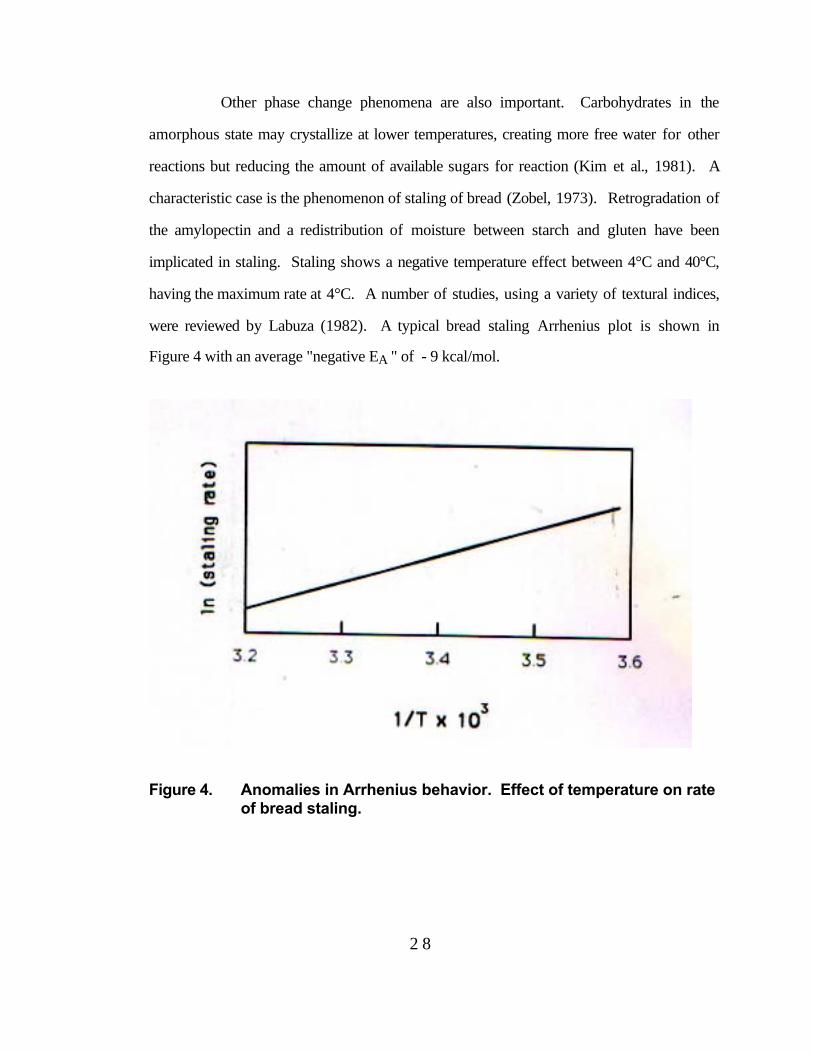
were reviewed by Labuza (1982). A typical bread staling Arrhenius plot is shown in
Figure 4 with an average "negative EA " of - 9 kcal/mol.
Figure 4. Anomalies in Arrhenius behavior. Effect of temperature on rateof bread staling.

2 9
Glass transition phenomena are also implicated in systems that, at certain
temperature ranges, deviate significantly from an Arrhenius behavior. Certain processing
conditions or drastic changes in storage conditions, such as rapid cooling and solvent
removal, result in formation of metastable glasses, especially in carbohydrate containing
foods (MacKenzie, 1977; Roos and Karel,1990; Levine and Slade,1988). Examples of
such foods include spray dried milk (Bushill,1965), boiled sweets (White and Cakebread,
1969), frozen solutions (MacKennzie, 1977), whey powder and dehydrated vegetables
(Buera and Karel, 1993).
Glass transition theory applicable to amorphous polymers has been used for
food polymers and compounds of smaller molecular weight. Amorphous glasses undergo
a glass to rubber transition at a temperature Tg. Above the glass transition temperature,Tg,
there is a drastic decrease in the viscosity (from an order of 1012 to 103 Pa.sec) (Ferry,
1980) and a substantial increase in the free volume i.e. the space which is not taken by
polymer chains themselves. This results in a greater polymer chain mobility and faster
reactant diffusion. Often the dependence of the rate of a food reaction on temperature,
when Tg is crossed, cannot be described with a single Arrhenius equation. A change of
slope (i.e. in activation energy) is observed at Tg. Furthermore, above Tg, in the rubbery
state, the activation energy may exhibit a temperature dependency, expressed as a gradually
changing slope in the Arrhenius plot. Williams, Landel and Ferry (1955) introduced the
WLF equation to empirically model the temperature dependence of mechanical and
dielectric relaxations within the rubbery state. It has been proposed (Slade et al, 1989) that
the same equation may describe the temperature dependence of of chemical reaction rates
within amorphous food matrices, above Tg. In diffusion controlled systems where
diffusion is free volume dependent, reaction rate constants can be expressed as function of
temperature by the WLF equation (Sapru and Labuza, 1992):

3 0
log( krefk ) =
C1(T-Tref) C2+(T-Tref) (36)
where kref the rate constant at the reference temperature Tref (Tref >Tg) and C1, C2 are
system-dependent coefficients. Williams et al (1955), for Tref=Tg, using experimental data
for different polymers, estimated average values of the coefficients: C1=-17.44 and
C2=51.6. In various studies these are used as universal values to establish the applicability
of WLF equation for different systems. This approach can be misleading (Ferry,1980;
Peleg, 1990; Buera and Karel,1993) and effort should be made to obtain and use system
specific values.
Alternative approaches for accessing the applicability of the WLF model and
calculating the values of C1 and C2 have been evaluated (Nelson, 1993; Buera and Karel,
1993). Eq. (36) can be rearranged into an equation of a straight line. Thus the plot of
[log kref
k ]-1 vs. 1
T-Tref is a straight line with a slope equal to C2/C1 and an intercept of
1/C1. If the glass transition temperature, Tg, is known, the WLF constants at Tg can be
calculated (Peleg,1992):
C1g= C1C2
C2+Tg-Tref and C2g=C2+Tg- Tref (37)
These values can be compared to the aforementioned average WLF coefficients.
When Tg and reaction rate data at many higher temperatures are available, kg,
C1 and C2 can be estimated from eq.(36) using non linear regression methodology.
Ferry (1980) proposed an additional approach for verifying the WLF
equation and determining the coefficients. A temperature T∞ , at which the rate of the
reaction is practically zero, is used. T∞ can be approximated by the difference between the
reference temperature and C2 i.e. T∞=Tref-C2. Rearranging eq. (36)
log( krefk ) =
C1(T-Tref) T-T∞ (38)

3 1
i.e. if T∞ is chosen correctly, a plot of log(k/kref) vs. (T-Tref)/(T-T∞) is linear through the
origin with slope equal to C1. Tg-50° C was proposed as a good initial estimate of T.
Buera and Karel (1993) used this approach to test the applicability of WLF equation in
modeling the effect of temperature on the rate of nonenzymatic browning, within several
dehydrated foods and carbohydrate model systems. Table 4 gives the calculated values of
the coefficients of the WLF equation for the different systems at the used reference
temperature as well as at Tg, for different moisture contents.

3 2
Table 4. WLF coefficients determined for several foods and model systems reportedat a reference temperature (C1 and C2) and transformed to correspond toTref = Tg (C1g and C2g) (Buera and Karel, 1993)
System Too Tref Tg moisture .C1 C2 C1g C2g( C) ( C) (g H20/g solid)
apple Tg-50 55 22 0.014 8.79 83 14.59 502 0.022 8.79 103 18.05 50
-7 0.050 8.79 112 19.69 50-13 0.087 8.70 118 20.73 50-24 0.011 8.79 129 22.68 50-38 0.017 8.79 143 25.14 50
cabbage Tg-50 45 15 0.014 7.82 80 12.5 505 0.021 7.82 90 14.07 501 0.032 7.82 94 14.7 50
-8 0.056 7.82 103 16.1 50-29 0.089 7.82 115 17.98 50-26 0.117 7.82 121 18.92 50-58 0.179 7.82 153 23.93 50
carrot Tg-50 43 -5 0.054 7.44 98 14.58 50-20 0.062 7.44 103 15.33 50-15 0.080 7.44 108 16.07 50
nonfat Tg-100 90 101 0.000 8.1 89 7.2 100dried milk 65 0.012 8.1 125 10.14 100
44 0.059 8.1 146 11.83 100nonfat Tg-100 90 50 0.030 6.8 140 9.52 100dried milk 45 0.040 6.8 145 9.86 100
40 0.050 6.8 150 10.2 100onion Tg-50 30 -8 0.056 8.8 88 15.9 50
-20 0.089 8.8 100 18.1 50-58 0.189 8.8 138 24.5 50
potato Tg-65 50 30 0.049 7.92 85 10.4 6520 0.094 7.92 95 11.6 65-5 0.150 7.92 120 14.6 65
-15 0.200 7.92 130 15.84 65whey powder Tg-100 35 29 0.059 8.4 106 9.0 100
18 0.080 8.4 117 9.9 100model sys1* Tg-90 45 45 0.059 8.3 90 8.3 90model sys2** Tg-10 55 40 0.073 6.93 135 7.8 120
* model system 1 composition: 99 % poly(vinyl pyrrolidone), 0.5 % glucose, 0.5 % glycine.** model system 2 composition: 98 % poly(vinyl pyrrolidone), 1 % xylose, 0.5 % lysine.
3 3
A number of recent publications debate the relative validity of the Arrhenius and
WLF equations in the rubbery state namely in the range 10 to 100° C above Tg. This
dilemma may very well be an oversimplification. (Karel,1993). As mentioned above,
processes affecting food quality that depend on viscosity changes (e.g. crystallization,
textural changes) fit the WLF model. However chemical reactions may be either kinetically
limited, when k<<αD (where D the diffusion coefficient and α a constant independent of
T) , diffusion limited when k>>αD or dependent on both when k and αD of the same
order of magnitude. In the latter case the effective reaction rate constant can be expressed
as k
1+k/αD . k in most cases exhibits an Arrhenius type temperature dependence and D
has been shown in many studies to either follow the Arrhenius equation with a change in
slope at Tg or to follow the WLF equation in the rubbery state and especially in the range
10 to 100° C above Tg. The value of the ratio k/αD defines the relative influence of k and
D and determines whether the deteriorative reaction can be successfully modeled by a
single Arrhenius equation for the whole temperature range of interest or a break in slope
occurs at Tg with a practically constant slope above Tg or with a changing slope in which
case the WLF equation will be used for the range 10 to 100° C above Tg. In complex
systems where multiple phases and reaction steps can occur, successful fit to either model
has to be considered as an empirical formula for practical use and not an equation
explaining the mechanism or phenomenon.
When several reactions with different EA's are important to food quality, it is
possible that each of them will predominantly define quality for a different temperature
range. Thus, for example, if quality is measured by an overall flavor score, the quality
change rate vs. 1/T will have a different slope in each of these regions. This is shown
schematically in Figure 5. A typical example of such a behavior is quality loss of

3 4
dehydrated potatoes where lipid oxidation and loss of fat soluble vitamins predominates up
to 31°C and nonenzymatic browning and lysine loss above 31°C (Labuza, 1982).
Figure 5. Typical temperature dependence of quality loss whenreactions of different EA affect quality.
The behavior of proteins at high enough temperature whereby they denature
and thus increase or decrease their susceptibility to chemical reactions depending upon the
stereochemical factors that affect these reactions, is another factor that can cause non-
Arrhenius behavior. For reactions that involve enzymatic activity or microbial growth the
temperature dependence plot shows a maximum rate at an optimum temperature, below and
above which an Arrhenius type behavior is exhibited. This is demonstrated in Figure 6.
Figure 6. Typical temperature dependence curve of an enzymaticreaction or microbial growth.

3 5
The study of the temperature dependence of microbial growth has lately been an area
of increased activity. The described kinetic principles are applied to compile the neccessary
data for modeling growth behavior, in a multidisciplinary field coded predictive
microbiology (Buchanan,1993; McClure et al., 1994; McMeekin et al., 1993). For a
temperature range below the optimum growth temperature either of the two simple
equations, Arrhenius and square root, sufficiently model the dependence for all practical
purposes (Labuza et al., 1991). The two-parameter empirical square root model, proposed
by Ratkowsky et al.(1982) has the form
k = b (T-Tmin) (39)
where k is growth rate, b is slope of the regression line of k vs temperature, and Tmin is
the hypothetical growth temperature where the regression line cuts the T axis at k =0.
The relation between Q10 and this expression is
Q10=
T-Tmin+10
T-Tmin
2(40)
Equations with more parameters, to model growth (and lag phase)
dependence through the whole biokinetic range, were also introduced, either based on the
square root model ( Ratkowsky et al., 1983) or the Arrhenius equation (Mohr and Krawiek,
1980 ; Scoolfield et al., 1981, Adair et al., 1989). They were reviewed and experimentally
evaluated by Zwietering et al. ( 1991).
Traditionally the mathematical models relating the numbers of microorganisms to
temperature have been divide into two main groups (Whiting and Buchanan, 1994): Those
describing propagation or growth primarily refer to the lower temperature range, and those
describing thermal destruction at lethal temperature range. Recently, a combined approach
utilizing a single mathematical formula to describe both the propagation and destruction
rate constant over the entire temperature range, from growth (k(T)>0) to lethality was

3 6
proposed (Peleg, 1995). The main applicability of such a model is to account for changes
that take place at a temperature range where transition from growth to lethality occurs.
Finally, temperature can have an additional indirect effect by affecting other
reaction determining factors, which will be discussed in the next section. A temperature
increase, increases the water activity at the same moisture level or enhances the moisture
exchange with the environment in cases of permeable packaging affecting the reaction rate.
Reactions that are pH-dependent can be additionally affected by temperature change, since
for many solute systems pH is a function of temperature (Bates, 1973). Solubility of
gases, especially of oxygen, changes with temperature (25% decrease with every 10°C
increase for O2 in water) thus affecting oxidation reactions where the oxygen is limiting.
10.2.2.2.Effects of other environmental factors
Moisture content and water activity (aw) are the most important Ej factors besides
temperature that affect the rate of food deterioration reactions. Water activity describes the
degree of boundness of the water contained in the food and its availability to act as a
solvent and participate in chemical reactions (Labuza, 1977).
Critical levels of aw can be recognized above which undesirable deterioration of
food occurs. Controlling the aw is the basis for preservation of dry and intermediate
moisture foods (IMF). Minimum aw values for growth can be defined for different
microbial species. For example, the most tolerant pathogenic bacterium is Staphylococcus
aureus , which can grown down to an aw of 0.85-0.86. This is often used as the critical
level of pathogenicity in foods. Beuchat (1981) gives minimum aw values for a number of
commonly encountered microorganisms of public health significance.
Textural quality is also greatly affected by moisture content and water activity.
Dry, crisp foods (e.g., potato chips, crackers) become texturally unacceptable upon gaining
moisture above the 0.35 to 0.5 aw range (Katz and Labuza, 1981). IMF like dried fruits
3 7
and bakery goods, upon losing moisture below an aw of 0.5 to 0.7, become unacceptably
hard (Kochhar and Rossel, 1982). Recrystallization phenomena of dry amorphous sugars
caused by reaching an aw of 0.35 - 0.4 affect texture and quality loss reaction rates, as
already mentioned.
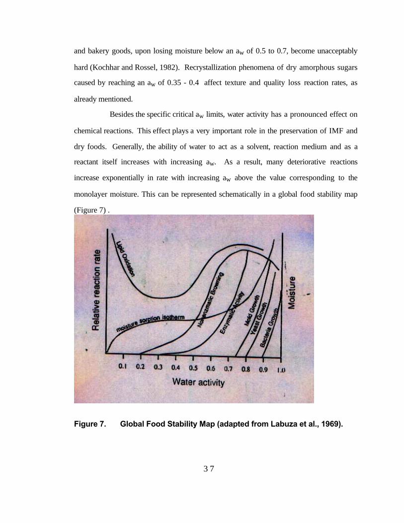
Besides the specific critical aw limits, water activity has a pronounced effect on
chemical reactions. This effect plays a very important role in the preservation of IMF and
dry foods. Generally, the ability of water to act as a solvent, reaction medium and as a
reactant itself increases with increasing aw. As a result, many deteriorative reactions
increase exponentially in rate with increasing aw above the value corresponding to the
monolayer moisture. This can be represented schematically in a global food stability map
(Figure 7) .
Figure 7. Global Food Stability Map (adapted from Labuza et al., 1969).
3 8
The critical aw limits for microbial growth and the relative rates of reactions
important to food preservation such as lipid oxidation and nonenzymatic browning can be
seen in this figure (Fig.7). The underlying reasons for this behavior has been the subject of
several studies (Taoukis et al., 1988a). Most reactions have minimal rates up to the
monolayer value. Lipid oxidation shows the peculiarity of a minimum at the monolayer
(mo) with increased rates below and above it (Labuza, 1975; Quast et al., 1972).
The proposed theories that attempt to explain the effect of aw on food
deterioration reaction as well as ways to systematically approach and model this effect are
discussed by Labuza (1980b). The moisture content and water activity can influence the
kinetic parameters (kA, EA), the concentrations of the reactants and in some cases even the
apparent reaction reaction order, n. Most relevant studies have modeled either kA as a
function of aw (Labuza, 1980b) related to the change of mobility of reactants due to aw
dependent changes of viscosity, or EA as a function of aw (Mizrahi, et al., 1970 a; b). The
inverse relationship of EA with aw (increase in aw decreases EA and vice versa) could be
theoretically explained by the proposed phenomenon of enthalpy-entropy compensation.
The applicability of this theory and data that support it have been discussed by Labuza
(1980a).
Additionally moisture content and aw directly affect the glass transition
temperature of the system. With increasing aw, Tg decreases. As was discussed in the
previous section, transverse of Tg and change into the rubbery state, has pronounced
effects, especially in texture and viscosity depended phenomena but also in reaction rates
and their temperature dependence. It has been proposed for dehydrated systems that a
critical mosture content / aw alternative to the monolayer value of the BET theory, is the
value at which the dehydrated system has a Tg of 25° C ( Roos,1993). Consideration of
these critical values contribute to explain textural changes occuring at distinct aw and
3 9
ambient temperatures (e.g loss of crispness of snack foods above 0.3-0.5 or unacceptable
hardness of IMF foods below 0.7-0.5) but their practical significance in aw dependent
chemical reactions is not straightforward and cannot be viewed isolated. Nelson and
Labuza (1994) reviewed cases where the fundamental assumption that reaction rates within
the ruberry state were dramatically higher than in the "stable" glassy state was not verified.
In complex systems, matrix porosity, molecular size, and phenomena such as collapse and
crystallization occuring in the rubbery state result in more complicated behavior. Both
water activity and glass transition theory contribute to explain the relationship between
moisture content and deteriorative reaction rates. It should be stressed though, that in
contrast to the well established moisture isotherm determination, i.e the moisture-aw
relation, accurate detremination of Tg as a function of moisture in a real food system is a
difficult task and an area where much more work is needed. Furthermore, caution should
be exercised when extrapolating state of the art knowledge to matters of safety. Water
activity, used as mentioned above as an index of microbial stability, is a well established
and practical tool in the context of hurdle technology. Additional criteria related to Tg
should be considered only after careful challenge and sufficient experimental evidence
(Chirife and Buera, 1994).
Mathematical models that incorporate the effect of aw as an additional
parameter can be used for shelf life predictions of moisture sensitive foods (Mizrahi et
al.,1970 a; Cardoso and Labuza, 1983, Nakabayashi et al., 1981). Such predictions can be
applied to packaged foods in conjunction with moisture transfer models developed based
on the properties of the food and the packaging materials (Taoukis et al., 1988b). Also
ASLT methods have been used to predict shelf life at normal conditions based on data
collected at high temperature and high humidity conditions (Mizrahi et al., 1970b).
The pH of the food system is another determining factor. The effect of pH on
different microbial, enzymatic and protein reactions has been studied in model biochemical

4 0
or food systems. Enzymatic and microbial activity exhibits an optimum pH range and
limits above and below which activity ceases, much like the response to temperature (Figure
6). The functionality and solubility of proteins depend strongly on pH, with the solubility
usually being at a minimum near the isoelectric point (Cheftel et al.,1985), having a direct
effect on their behavior in reactions.
Examples of important acid-base catalyzed reactions are nonenzymatic
browning and aspartame decomposition. Nonenzymatic browning of proteins shows a
minimum near pH=3-4 and high rates in the near neutral-alkaline range (Feeney et al.,
1975; Feeney and Whitaker, 1982). Aspartame degradation is reported at a minimum at
pH=4.5 (Holmer, 1984), although the buffering capacity of the system and the specific
ions present have significant effect (Tsoumbeli and Labuza, 1991). Unfortunately very few
studies consider the interaction between pH and other factors e.g temperature. Such
studies (Bell and Labuza, 1991and1994; Weismann et al., 1993) show the significance of
these interactions and the need for such information for the design and optimization of real
systems. Significant progress in elucidating and modeling the combined effect to
microbial growth of factors such as T, pH, aw or salt concentation has been achieved in the
field of predictive microbiology ( Ross and McMeekin, 1994; Rosso et al., 1995)
Gas composition also affects certain quality loss reactions. Oxygen affects
both the rate and apparent order of oxidative reactions, based on its presence in limiting or
excess amounts (Labuza, 1971). Exclusion or limitation of O2 by nitrogen flushing or
vacuum packaging reduces redox potential and slows down undesirable reactions.
Further, the presence and relative amount of other gases, especially carbon dioxide, and
secondly ethylene and CO, strongly affects biological and microbial reactions in fresh
meat, fruit and vegetables. The mode of action of CO2 is partly connected to surface
acidification (Parkin and Brown, 1982) but additional mechanisms, not clearly established,
are in action . Quantitative modeling of the combined effect on microbial growth of

4 1
temperature and is an area of current research (Willocx et al., 1993). Different systems
require different O2 - CO2 - N2 ratios to achieve maximum shelf life extension. Often
excess CO2 can be detrimental. Alternatively, hypobaric storage, whereby total pressure is
reduced, has been studied. Comprehensive reviews of controlled and modified atmosphere
packaging (CAP/MAP) technology are given by Kader (1986); Labuza and Breene (1988)
and Farber (1991). Bin et al. (1992) review the efforts that have focused on kinetically
modeling the CAP/MAP systems.
Currently experiments with very high pressure technology (1,000 to 10,000 atm)
are being conducted. This hydrostatic pressure, applied via a pressure transfering medium,
acts without time delay and is independent of product size and geometry. It can be
effective at ambient temperatures (Hoover, 1993). Key effects sought from high pressure
technology include (Knorr, 1993): a) Inactivation of microorganisms, b) modification of
biopolymers (protein denaturation, enzyme inactivation or activation, degradation), c)
increased product functionality (e.g. density, freezing temperatures, texture) and d) quality
retention (e.g. color, flavor due to the fact that only nonvalent bonds are affected by
pressure). Kinetic studies of changes occurring during high pressure processing and their
effects on shelf life of the foods are very limited and further research will be needed for
this technology to be fully utilized.
To express the above diccussed effect of different factors in a simple
mathematical form, the concept of the quality function can be used in a more general
approach. Assuming that the quality of the food depends on i different quantifiable
deterioration modes (quality factors), Ai, respective quality functions can be defined in
analogy to Eq.14.
Qi(Ai) = ki t (41)
The rate constant ki of each particular deterioration mode is a function of the
aforementioned factors, namely

4 2
ki = f (T,aw,pH, PO2, PCO2
...) (42)
the values of which are in turn time dependent:
T=T(t), aw = aw(t), pH=pH(t), PO2= PO2
(t), PCO2= PCO2
(t) (43)
The functions of (32) incorporate the effects of storage conditions, packaging
method and materials and biological activity of the system. Thus for variable conditions
the rate constant is overall a function of time, i.e. ki=ki(t). In that case the quality function
value at certain time is given by the expression
Qi(Ai) =⌡⌠0
tki dt (44)
If the lower acceptable value of the quality parameter Ai, noted as Am is known
then at time t the consumed quality fraction, Φci , and the remaining quality fraction, Φri ,
are defined as:
Φci= Qi(Ai)-Qi(Ao)Qi(Am)-Qi(Ai) (45)
Φri= Qi(Am)-Qi(Ai)Qi(Am)-Qi(Ao) (46)
Knoweledge of the value of Φri for the different deterioration modes allows the calculation
of the remaining shelf life of the food, θr, from the expression
θr= min [ Φri/ki] (47)
where the rate constants ki are calculated for an assumed set of "remaining" constant
conditions.
The above analysis sets the foundations of shelf life prediction of a complex
system under variable conditions. The major tasks in a scheme like this, is recognition of
the major deterioration modes, determination of the corresponding quality functions and
estimation of Eq.(42) i.e. the effects of different factors on the rate constant. The latter is a
difficult task for real food systems. Most actual studies concern the effect of temperature
4 3
and variable temperature conditions, with the expressed (or implied) assumption that the
other factors are constant. Controlled temperature functions like square, sine, and linear
(spike) wave temperature fluctuations can be applied to verify the Arrhenius model,
developed from several constant-temperature shelf life experiments . Labuza (1984) gives
analytical expressions for Eq. (44) for the above temperature functions using the Q10
approach. Similarly solutions can be given using the Arrhenius or square root models.
To systematically approach the effect of variable temperature conditions the
concept of effective temperature, Teff, can be introduced. Teff is a constant temperature that
results in the same quality change as the variable temperature distribution over the same
period of time. Teff is characteristic of the temperature distribution and the kinetic
temperature dependence of the system. The rate constant at Teff is analogously termed
effective rate constant, and Qi(Ai) of Eq.(44) is equall to keff t. If Tm and km are the mean
of the temperature distribution and the corresponding rate constant respectively, the ratio Γ
is also characteristic of the temperature distribution and the specific system, where
Γ=keffkm
(48)
For some known characteristic temperature functions shown in Fig.8 analytical
expressions for the Q10 and Arrhenius models are tabulated in Table 5.

4 4
Table 5. Analytical expressions for calculation of Γ for different temperature functions.
Function Q10 Approach Arrhenius Approach
Sine wave
Γ=Io (aob) Γ ≈ I oEaao
RTm Tm+ao
Square wave
Γ=12 [eaob+e-aob] Γ=
12 exp[
EAaoRTm(Tm+ao) ] +
12 exp[
-EAaoRTm(Tm-ao) ]
Spike wave Γ= eaob-e-aob
2aob Γ=exp[
EAaoRTm(Tm+ao)] - exp[
-EAaoRTm(Tm-ao)]
2EAao
RTm(Tm+ao)
Random Γ=
∑j=0
n
ebTj ∆tj
ebTm Γ=
∑j=0
n
exp(-EA
RTj) ∆tj
exp(-EA
RTm)
Io(x) is a modified Bessel function of zero order. Its values can be calculated from an
infinite series expansion, Io(x)=1+x2
22 +x4
2242 + x6
224262 +..., or found in Mathematical
Handbooks (Tuma, 1988).
From Γ of a variable temperature distribution the effective reaction rate and
temperatures keff andTeff and the value of the quality function for the particular
deterioration mode are calculated. Comparison of this value to the experimentally obtained
quality value, for variable temperature functions covering the range of practical interest is
the ultimate validation of the developed kinetic models. This methodology was applied by
Labuza and coworkers for various food reaction systems and agreement or deviation from
predicted kinetic behavior was assessed (Berquist and Labuza, 1983; Kamman and
Labuza,1981; Labuza et al. 1982; Riboh and Labuza, 1982; Saltmarch and Labuza,1982;
Taoukis and Labuza,1989).

4 5
Figure 8. Characteristic fluctuating temperature distributions used toverify validity of kinetic models. ao is the amplitude of the sine,square and spike wave functions.
Alternatively the effect of variable temperature distribution can be expressed
through an equivalent time (teq), defined as the time at a reference temperature (is) resulting
in the same quality change (i.e. same value of quality function) as the variable temperature.
The practicality of teq is that if the chosen Tref is the suggested keeping temperature e.g.
4°C for chilled products, it will directly give the remaining shelf life at that temperature.
Note that if the mean temperature is chosen as the reference temperature, Tref=Tm, then
teq/t=Γ.
Further a short mention of the Equivalent point method is relevant. This
approach has been used for evaluation and modelling of thermal processes (Nunes and
Swartzel, 1990) and the response of Time Temperature Indicators (TTI) (Fu and Labuza,
1993). The same methodology would apply for quality loss during the shelf life of foods.
Using the expression of the quality function

4 6
Q(A)= kA exp (- EART ) t (49)
and if Y=Q(A)/kA then the above equation can be written as
lnY= -1RT EA + lnt (50)
i.e a plot of lnY vs EA of different food systems gives a straight line. For a particular
variable time-temperature distribution it is proposed that a unique point (Te,te) is defined
from the slope and intercept of Eq.(50). This would allow calculation of the quality change
in a food system of known EA from the measured change of two (at least) other food
systems (or TTI) subjected to the same time -temperature conditions. It has been recently
argued that this approach is only valid for isothermal conditions (Maesmans et al., 1995).

4 7
10.3 APPLICATION OF FOOD KINETICS IN SHELF LIFE PREDICTION AND
CONTROL
10.3.1.Accelerated Shelf Life Testing
Taking into account the described limitations and the possible sources of deviation, the
Arrhenius equation can be used to model food degradation for a range of temperatures.
This model can be used to predict reaction rates and shelf life of the food at any
temperature within the range, without actual testing. Equally important it allows the use of
the concept of accelerated shelf life testing (ASLT).
ASLT involves the use of higher testing temperatures in food quality loss and
shelf life experiments and extrapolation of the results to regular storage conditions through
the use of the Arrhenius equation. That cuts down very substantially the testing time. A
reaction of an average EA of 90 kJ/mol may be accelerated by 9 to 13 times with a 20°C
increase in the testing temperature, depending on the temperature zone. Thus an
experiment that would take a year can be completed in about a month. This principle and
the methodology in conducting effective ASLT are described by Labuza (1985), Labuza
and Schmidl (1985), and in a publication by the Institute of Food Science and Technology,
UK (IFST,1993).
Designing a shelf life test is a synthetic approach that requires sufficient
understanding of all food related disciplines, namely food engineering food chemistry,
food microbiology, analytical chemistry, physical chemistry, polymer science and food
regulations. The following steps outline the ASLT procedure:
1. Evaluate the microbiological safety factors for the proposed food product and
process. Use of the Hazard Analysis Critical Control Point (HACCP) principles is a good
approach to be followed from the design stage. If major potential problems exist at this
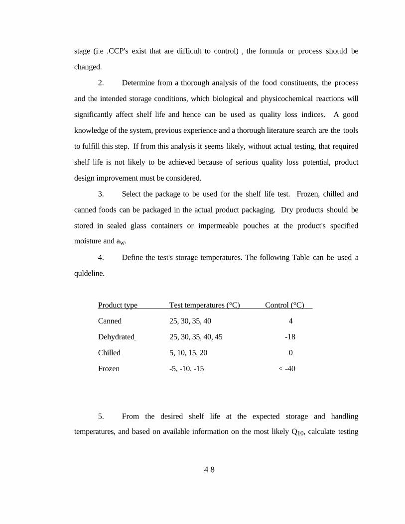
4 8
stage (i.e .CCP's exist that are difficult to control) , the formula or process should be
changed.
2. Determine from a thorough analysis of the food constituents, the process
and the intended storage conditions, which biological and physicochemical reactions will
significantly affect shelf life and hence can be used as quality loss indices. A good
knowledge of the system, previous experience and a thorough literature search are the tools
to fulfill this step. If from this analysis it seems likely, without actual testing, that required
shelf life is not likely to be achieved because of serious quality loss potential, product
design improvement must be considered.
3. Select the package to be used for the shelf life test. Frozen, chilled and
canned foods can be packaged in the actual product packaging. Dry products should be
stored in sealed glass containers or impermeable pouches at the product's specified
moisture and aw.
4. Define the test's storage temperatures. The following Table can be used a
quldeline.
Product type Test temperatures (°C) Control (°C)
Canned 25, 30, 35, 40 4
Dehydrated 25, 30, 35, 40, 45 -18
Chilled 5, 10, 15, 20 0
Frozen -5, -10, -15 < -40
5. From the desired shelf life at the expected storage and handling
temperatures, and based on available information on the most likely Q10, calculate testing

4 9
time at each selected temperature. If no information is available on the expected Q10 value,
minimum three testing temperatures should be used.
6. Decide the type and frequency of tests to be conducted at each temperature.
A useful formula to determine the minimum frequency of testing at all temperatures based
on the testing protocol at the highest temperature
f2=f1 Q10∆T/10 (51)
where f1 is the time between tests (e.g., days, weeks) at highest test temperature T1; f2 is the
time between tests at any lower temperature T2; and ∆T is the difference in degrees Celsius
between T1 and T2. Thus, if a canned product is held at 40°C and tested once a month,
then at 30°C (i.e ∆T=5) and a Q10 of 3, the product should be tested at least every 1.73
months. Usually, more frequent testing is recommended, especially if the Q10 is not
accurately known. Use of too long intervals may result in an inaccurate determination of
shelf life and invalidate the experiment. At each storage condition, at least six data points
are required to minimize statistical errors; otherwise, the statistical confidence in the
obtained shelf life value is significantly reduced.
7. Plot the data as it is collected to determine the reaction order and to decide
whether test frequency should be altered. It is a common practice for the data not to be
analyzed until the experiment is over and then it is recognized that changes in the testing
protocol, affected early on, would have added significantly to the reliability of the results.
8. From each test storage condition, determine reaction order and rate, make
the appropriate Arrhenius plot, and predict the shelf life at the desired actual storage
condition. Product can also be stored at the final condition, to determine its shelf life and
test the validity of the prediction. However, in industry this is uncommon because of time
and cost constraints. It is a much more effective and realistic practice to test the obtained

5 0
predictive shelf life model by conducting an additional test at a controlled variable
temperature. The results will be compared to the predicted values according to Table 5.
Mathematical models that incorporate the effect of aw as an additional
parameter can be used for shelf life predictions of moisture sensitive foods. Such
predictions can be applied to packaged foods in conjunction with moisture transfer models
developed based on the properties of the food and the packaging materials (Taoukis et al.,
1988b). Also ASLT methods have been used to predict shelf life at normal conditions
based on data collected at high temperature and high humidity conditions (Mizrahi et al.,
1970b). Weissman et al. (1993) propose a novel approach for ASLT whereby not only
external conditions but concentration of selected reactants or catalysts are used to accelerate
the storage test. When this is feasible high acceleration ratios can be achieved and testing
times can be reduced significantly.
10.3.2 Use of Time Temperature Indicators as shelf life monitors
Generally a Time-Temperature Indicator (TTI) can be defined as a simple,
inexpensive device that can show an easily measurable, time-temperature dependent change
that reflects the full or partial temperature history of a (food) product to which it is
attached. TTI operation is based on mechanical, chemical, enzymatic or microbiological
systems that change irreversibly from the time of their activation. The rate of change is
temperature dependent, increasing at higher temperatures in a manner similar to most
physicochemical reactions. The change is usually expressed as a visible response, in the
form of a mechanical deformation, colour development or colour movement. The visible
reading thus obtained gives some information on the storage conditions that have preceded
it. The ability of TTI to function as cumulative recorders of temperature history from their
activation time to the time each response measurement is taken, make them useful for two
types of applications.
5 1
TTI can be used to monitor the temperature exposure of individual food
packages, cartons or pallet loads during distribution up to the time they are displayed at the
supermarket. By being attached to individual cases or pallets they can give a measure of
the preceding temperature conditions at each receiving point. These points would serve as
information gathering and decision making centres. The information gathered from all
stations could be used for overall monitoring of the distribution system, thus allowing for
recognition and possible correction of the more problematic links.
The second type of TTI application involves their use as quality monitors.
With quality loss being a function of temperature history and with TTI giving a measure of
that history, their response can presumably be correlated to the quality level of the food. If
that can be achieved, TTI can be used in either (or both) of two ways. The first would be as
an inventory management and stock rotation tool at the retail level. The approach used
presently is the First In First Out (FIFO) system according to which, products received
first and/or with the closest expiration date on the label are displayed and sold first. This
approach aims in establishing a "steady state" with all products being sold at the same
quality level. The assumption is that all products have gone through uniform handling,
thus quality is basically a function of time. The use of the indicators can help establish a
system that does not depend on this unrealistic assumption. The objective will again be the
reaching of a "steady state" situation with the least remaining shelf life products being sold
first. This approach could be coded LSFO (Least Shelf-life First Out). The LSFO system
could theoretically (although not proven) reduce rejected products and eliminate consumer
dissatisfaction since the fraction of product with unacceptable quality sent into the
distribution system will be eliminated. Secondly, TTI attached on individual packaged
products, can serve as dynamic or active shelf life labeling instead of (or in conjunction
with) open date labeling. The TTI would assure the consumers that the products were

5 2
properly handled and would indicate remaining shelf life. Use of TTI as "consumer
indicators" is the ultimate goal of these systems.
A variety of TTI based on different physicochemical principles have been
described by Byrne (1976) and Taoukis et al.(1991). Statistical correlations of TTI
performance and product quality characteristics have been reported for a variety of
perishable and frozen foods (Tnker et al.,1985; Chen and Zall,1987; Wells and
Singh,1988). A general approach that allows the correlation of the response of a TTI to the
quality changes of a food product of known deterioration modes, without actual
simultaneous testing of the indicator and the food, was developed by Taoukis and Labuza
(1989a). Three types of TTI commercially available were mathematically modeled using
Arrhenius kinetics. One type is based on a time-temperature depended diffusion of a dye
along a wick , the second on a change of color due to a controlled enzymatic reaction and
the third on development of color based on a solid state polymerization . A scheme was
introduced that allows the correlation of the TTI response, X, to the quality index A of the
food. X can be expressed as a function of time:
F(X)t = k t = kI exp(-EA / RT) t (52)
where F(X) is the response function of the TTI, t is the time and k the response rate
constant; the constant kI and the activation energy EA are the Arrhenius parameters. For a
TTI going through the same temperature distribution, T(t) as the monitored food, the value
of F(X)t is known from the response X ; Teff can then be calculated from equation (14)
for T=Teff. Teff and knowledge of the kinetic parameters of deterioration of the food
allows the evaluation of Q(A) and hence the quality loss of the product. The reliability of
the TTI under variable temperature conditions was also assessed(Taoukis and Labuza,
1989b), using the relations of Table 5, and in general was judged satisfactory.
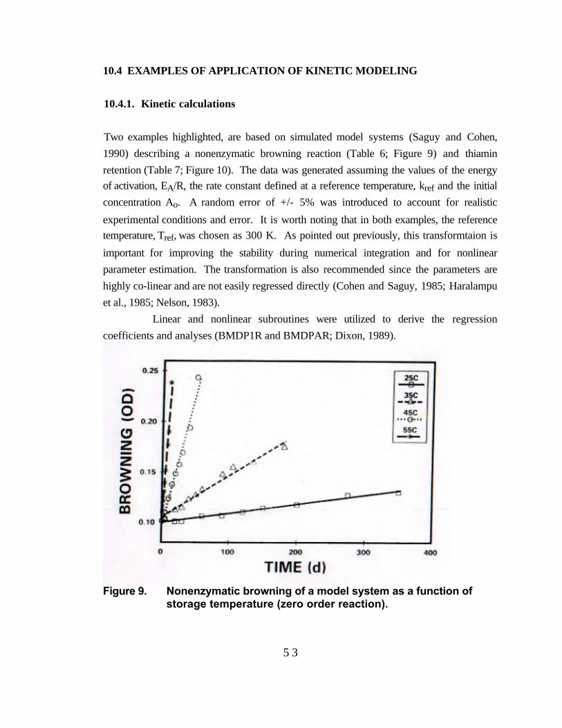
5 3
10.4 EXAMPLES OF APPLICATION OF KINETIC MODELING
10.4.1. Kinetic calculations
Two examples highlighted, are based on simulated model systems (Saguy and Cohen,
1990) describing a nonenzymatic browning reaction (Table 6; Figure 9) and thiamin
retention (Table 7; Figure 10). The data was generated assuming the values of the energy
of activation, EA/R, the rate constant defined at a reference temperature, kref and the initial
concentration Ao. A random error of +/- 5% was introduced to account for realistic
experimental conditions and error. It is worth noting that in both examples, the reference
temperature, Tref, was chosen as 300 K. As pointed out previously, this transformtaion is
important for improving the stability during numerical integration and for nonlinear
parameter estimation. The transformation is also recommended since the parameters are
highly co-linear and are not easily regressed directly (Cohen and Saguy, 1985; Haralampu
et al., 1985; Nelson, 1983).
Linear and nonlinear subroutines were utilized to derive the regression
coefficients and analyses (BMDP1R and BMDPAR; Dixon, 1989).
Figure 9. Nonenzymatic browning of a model system as a function ofstorage temperature (zero order reaction).

5 4
Table 6 Simulated nonenzymatic browning data (1) as a function of storage temperature
for Figure 9
Time Nonenzymatic browning (OD/g solid) for temperatures
(days) 25 °C 35 °C 45 °C 55 °C
1 0.102 0.1112 0.1213 0.1314 0.1395 0.103 0.104 0.110 0.1528 0.1779 0.19010 0.12411 0.23815 0.13720 0.101 0.112 0.14825 0.15830 0.101 0.114 0.16940 0.123 0.19450 0.127 0.24460 0.106 0.13390 0.107 0.148105 0.155120 0.110135 0.160150 0.114180 0.175200 0.117275 0.127350 0.130
(1) Adopted from Saguy and Cohen (1990).

5 5
Figure 10. Thiamin retention of a model system as function of storagetemperature (first-order reaction).
Table 7 Simulated thiamin retention (1) for a model system as a function of storagetemperature (first - order reaction) for Figure 10
Time Thiamin concentration (mg/g solid) for temperatures
(days) 25 °C 35 °C 45 °C 55 °C
1 96.70 93.402 85.475 98.22 0.104 89.44 69.928 54.6010 80.98 47.5012 42.2915 72.36 33.4320 98.16 0.112 66.7225 59.91 14.8030 94.80 0.114 51.9340 0.123 44.1150 0.12760 92.56 0.133 28.6290 88.61 0.148105 0.155120 85.84135 0.160150 81.27180 0.175197 76.29257 70.55300 67.15
(1) Adopted from Saguy and Cohen (1990).
5 6
A. Two-step method
The most common method to estimate the Arrhenius' parameters is the classic
succesive two-steps ordinary linear least squares fit. The first step is the regression of the
quality function (Table 1; i.e., Ao for zero-order, or ln (At/Ao) for a first-order reaction) vs.
time, at each temperature, to estimate the rate constant k, and the initial concentration Ao.
The estimation of Ao avoids bias in the determination, and provides an additional croiterion
of the adequacy of the model to describe the experimental data. A significant descrepancy
between the estimated and experimental Ao suggests that a problem exists. The problem
may be due to an inadequate kinetic model, large experimental error, insufficient number of
data, etc. The second step is regression of ln(k) vs. [1/T - 1/Tref] to obtain the estimated of
kref and EA/R.
B. Non-linear Least Squares (one step method)
The nonlinear regression performs a single regression an all of the data points
(i= 1, ....,n), to estimate EA/R, kref and Ao, without calculating the rates for each
temperature.
C. Results
The Arrhenius' parameters and the initial concentration derived using the two
regression methods are summarized in Table 8 for nonenzymatic browning (zero-order)
and thiamin (first-order) kinetics.
The results show no substantial differences among the derived values of EA/R
and kref when Methods 1 and 2 were applied. Nevertheless, the values derived by method 2
are closer to the actual values used for the simulation.
D. Confidence contour
As mentioned before the confidence contour for Ea/R and kref can be derived
using a computer program (Draper and Smith, 1981) which incorporates approximation
for a nonlinear regression of Eq.(27):

5 7
S = SS { 1+Np
n-Np F[Np, n-Np, (1-q)]} (27)
where f is the fitted nonlinear model, SS is the nonlinear least square estimate
of the fitted model, i.e. SS= Σ[ln(Ai-f)]2 for i=1 to n , n is the number of data points, Np
the number of parameters derived from the nonlinear least squares, 100(1-q)% the
confidence level and F the F -statistics.
The values used for deriving the confidence contour for the nonlinear
regression of the nonenzymatic browning data were as follows (Table 8):
SS=1.331 E-3; EA/R=15,796; Ao=99.32 and F(3,34,90%)=2.27.
The fitted model, f, is replaced with the appropriate model based on the reaction order:
zero-order
f = Ao + t exp
-EAR
1
T - 1
Tref
first order
f = exp
ln(Ao) + t exp
-EAR
1
T - 1
Tref
n - order (n not equal to 1)
f =
Ao(n-1) + (1-n) t exp
-EAR
1
T - 1
Tref(1/(1-n))
The appropriate sign +/- in the above equations should be chosen. For a
reaction where concentration increases a positive should be used. For a depletion reactrion
the negative sign should be utilized.
The algorithm implemented to derive the confidence region is as follows:
a. Initial concentration is assumed constant and the estimated value derived by the
nonlinear regression is utilized.
b. The confidence contour is derived by choosing values of EA/R and kref which fulfill
the equality expressed in Eq. (27). Obviously, the value of EA/R and kref are varied within
the range of values that satisfies the inequality listed in Eq. (27). This trial and error
procedure is normally carried out on a computer.
The derived confidence contour is depicted in Fig. 11. It shows the span in the
calculated values of EA/R and kref. When comparing the confidence regions derived by the

5 8
two regression methods. The nonlinear regression yields typically a smaller confidence
region. This means that a better estimation of shelf-life prediction and simulation is
possible (Cohen and Saguy, 1985; Haralampu et al., 1985).
Table 8 Effect of the regression method on the Arrhenius parameters derived for
nonenzymatic browning (zero-order) and thiamin retention (first - order reaction)
Regression df(a) k x 100 (b) EA/R kref(c) Ao(d) Aoavr(e)
method 25 °C 35°C 45°C 55°C 25 °C 35°C 45°C 55°C
Nonenzymatic Browning
Simulated values 15000 13.5 0.100
Two steps 1 9.1 41.6 270.21157.9 16067 11.7 0.100 0.105 0.095 0.098 0.098
Non-linear 19 - - - - 15796 12.2 - - - - 0.099
Thiamin retention
Simulated values 13000 0.178 100.0
Two steps 2 0.133 0.580 2.065 7.588 13125 0.17599.7 100.4 99.2 101.5 100.2
Non-linear 16 - - - - 12985 0.182 - - - - 99.8
(a) Degrees of freedom(b) Reaction rate constant: OD/g/day or day-1 for a zero and first order reaction, respectively(c) Units of kref at 300 K as in b above(d) Derived initial concentration: OD/g or mg/g thiamin for a zero and first order reaction respectively(e) Average of the derived initial concentration. Units as in d above
Figure 11. Joint confidence contour (90%) for EA/R and kref derived byone-step nonlinear least squares method, for nonenzymaticbrowning.

5 9
10.4.2. Examples of shelf life modeling of food products
The preceeding kinetic calculation cases show how judiciously we should use the kinetic
parameters we obtain from shelf life experiments. In most practical cases the two step
method is used due to its simplicity and convenience. The results should be understood as
mean values with possibly large confidence limits, and treated as such. Nevertheless, the
information obtained from carefully designed shelf life testing, at three or more
temperatures, is usually sufficient to allow derivation of satisfactory shelf life predicive
models. Further two examples that illustrate the use of ASLT principles and kinetic
modeling. The first, a commercially sterilized, flavored dairy beverage, sweetened with the
sweetener aspartame, is a case of straightforward use of these principles, as the quality
function of the food is defined by a dominant , quantifiable quality index, aspartame. In
contrast, the second example, of a complex food system of many antagonizing quality
deterioration modes illustrates the multidisciplinary approach and the deep knowledge of
the system required for effective shelf life testing.
10.4.2.1 Aspartame sweetened chocolate drink.
This practical example is based on experimental data generated in studies by
Bell and Labuza (1994) and Bell et al. (1994). These studies were intended to evaluate the
aspartame stability in commercially sterilized skim milk beverages of various compositions.
There is a steadily growing market for nutritious, low calorie dairy products, and aspartame
as a high intensity sweetener, without the controversy surrounding saccharin, can be a very
desirable ingredient. However, at the inherent pH of milk (6.6) the rate of aspartame
degradation is very high, reducing significantly the sensory shelf life of the product
Quantifying and modeling the behavior of this dominant quality index would allow
optimization of the product formulation and extension of shelf life, possibly by slight
alteration of the pH. For that purpose different commercially sterilized skim milks,
sweetened with 200 ppm of aspartame and slightly buffered with citrates or phosphates to
pH ranging from 6.38 to 6.67 were studied with regards to the aspartame degradation.
Samples were stored at 5 temperatures from 0 to 30° C and triplicate samples were
analyzed by HPLC, at appropriately spaced time intervals ( based on Eq.(51) and an
average Q10 value of 4 from the literature). Results of these experiments (at pH 6.67 with
.008 M citrate) are listed in Table 9.

6 0
Table 9. Aspartame degradation in a pH 6.67 aseptic dairy system
Time Aspartame concentration (ppm) for temperatures
(hr) 30 °C 20 °C 10 °C 4 °C 0 C
10 18110 17510 18223 168 18623 166 17223 171 18138 13038 12738 14148 120 15248 101 16048 108 16278 17278 15478 15395 17595 17395 175121 168 189 198121 168 180 195121 167 186 194143 146143 129143 150262 63 140 165262 73 134 165262 94 160 167455 114 132 159455 96 117 152455 118 121 155599 93 110 136599 87 104 136599 91 88 134694 80 130694 95 119694 86 113767 115767 109767 103

6 1
In Fig. 12a aspartame concentration (APM or A) is plotted vs. time at the 5
temperatures. The best linear fit of the form Q(A)=kt was achieved for Q(A)=ln(A/A o),
i.e. first order kinetics (Fig.12b). All measurements were included in the statistical analysis
(no averaging of the 3 samples per time) to increase the degrees of freedom and include the
measurement spread in the model. Calculated rate constants and 95% C.I. are given in
Table 10.
Table 10. Aspartame degradation reaction rate constants with confidence intervals at 5
temperatures.
Rate constant 30o C 20o C 10o C 4o C 0o C
-k (hr-1) 0.0125 0.00356 0.00138 0.00121 0.000790
± 95% C.I. ± 0.0013 ± 0.00046 ± 0.00010 ± 0.00009 ± 0.000062
Figure 12. Aspartame degradation kinetics at five temperatures plot asfunction of time and as semi-log plot
To determine the Arrhenius parameters, -k is plotted in a semilogarithmic scale
vs.the inverse of absolute temperature (or ln(-k) vs. 1/T). To increase the degrees of
freedom and get a narrower confidence interval for the calculated parameters, the 95% C.I.
for k are included (Fig. 13). The Arrhenius plot gives by linear regression the values of
ko=3.163 108 hr-1 and activation energy EA= 14560 cal/mol. The coefficient of
determination, R2, is 0.952 and the 95% confidence interval 1830 cal/mol.

6 2
Figure 13. Aspartame degradation kinetics plotted as Arrhenius relation
The obtained kinetic information allows the prediction of aspartame degradation
and thus the shelf life of the product for any keeping temperature. Thus, if one assumes
that the product is overcompensated with aspartame at 0 time to allow for acceptable
product sweetness up to the point that half of the sweetener is degraded, the shelf life at 4o
C is approximately 4 weeks (670 hr). Remaining shelf life can also be calculated after
exposure at any known temperature conditions. As an example, it is assumed that the
aseptic milk product is exposed for ten days the temperature conditions shown in Figure
14. It is a non specific variable distribution with a mean temperature,Tm, of 7.1o C. The
total aspartame degradation at the end of the 10 days can be calculated by integration. Thevalue of ratio Γ (Eq.48 and Table 5) is determined as 1.0437. At Tm after 10 days, the
remaining aspartame is 71.7%. Thus the actual aspartame level is calculated as 68.7%.
This can further be translated to remaining shelf life at constant 4o C of 307 hr (12.8 days).
Note that if the product was assumed to have remained at 4o C at the first 10 days, the
remaining shelf life would be 18 days.
The practical value of the described approach is that it allows a systematic
approach to shelf life prediction and optimization. Indeed similar results at the other
studied pHs showed activation energies in the range of 14 to 18 kcal/mol and shelf lifes
that reached 60 days at the lower end of pH range of 6.38. This is a valuable indication of
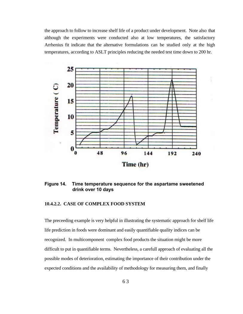
6 3
the approach to follow to increase shelf life of a product under development. Note also that
although the experiments were conducted also at low temperatures, the satisfactory
Arrhenius fit indicate that the alternative formulations can be studied only at the high
temperatures, according to ASLT principles reducing the needed test time down to 200 hr.
Figure 14. Time temperature sequence for the aspartame sweeteneddrink over 10 days
10.4.2.2. CASE OF COMPLEX FOOD SYSTEM
The preceeding example is very helpful in illustrating the systematic approach for shelf life
life prediction in foods were dominant and easily quantifiable quality indices can be
recognized. In multicomponent complex food products the situation might be more
difficult to put in quantifiable terms. Nevertheless, a carefull approach of evaluating all the
possible modes of deterioration, estimating the importance of their contribution under the
expected conditions and the availability of methodology for measuring them, and finally
6 4
using a judiciously developed testing protocol based on the principles developed in this
chapter. The "ultimate" example of food were such an approach is neededis fozen pizza.
All the aspects affecting the quality of this product were detailed by Labuza and Schmidl,
1985 and Labuza, 1985. Systems to be considered for monitoring chemical changes in
pizza during frozen storage include: Total free fatty acids, specific volatile free fatty acids
by GLC, peroxides, oxidative volatiles (e.g., hexanal) by GLC, spice volatiles by GLC,
lysine, color (decrease in red color or increase in brown), sensory properties: taste and
flavor, and nutrient loss such as vit. A and C. Physical changes such as loss of crust
crispness, loss of cheese functionality and meltability and development of in- package ice
must also be considered. Finally, microbiological changes cannot be neglected especillay
uder abuse senarios.
Detailed analysis of the relative contribution of the above factors and a proposed
testing protocol can be found in the referenced sources.

6 5
REFERENCES
Arabshashi, A. (1982). Effect and interaction of environmental and composition variables
on the stability of thiamin inintermediate moisture model systems.Ph.D. Thesis,
University of Wisconsin, Madison, Wisconsin.
Arabshashi, A. and D.B. Lund (1985). Considerations in calculating kinetic parameters
from experimental data. J. Food Proc. Engi. 7: 239-251.
Bates, R. G. (1973) "Determination of pH: Theory and Practice", 2nd ed. John Wiley
and Sons, New York, NY.
Bell, L.N. and T.P.Labuza (1991) Aspartame degradation kinetics as affected by pH in
intermediate and low moisture food systems. J. Food Sci. 56: 17-20.
Bell, L.N. and T.P.Labuza (1994). Influence of the low-moisture state on pH and its
implications for reaction kinetics. J.Food Eng. 22: 291-312.
Bell, L.N. and T.P.Labuza (1994). Aspartame stability in commercially sterilized flavored
dairy beverages. J.Dairy Sci. 77: 34-38.
Bell, L.N., Shoeman, D., Tsoubeli, M. and T.P.Labuza (1994). Kinetics of aspartame
degradation in liquid dairy beverages. In: Developments in Food Engineering:
Proceedings of the 6th Int. Congress on Engineering and Food. ( Yano, T.
Matsuno, R., Nakamura K. eds.) pp.489-491.
Benson, S.W. (1960). Foundations of Chemical Kinetics, McGraw-Hill, New York.
Bergquist, S., and T.P. Labuza (1983). Kinetics of peroxide formation in potato chips
undergoing a sine wave temperature fluctuation. J. Food Sci. 43:712.
Beuchat, L. R. (1981) Microbial stability as affected by water activity. Cereal Foods
World 26, 345-349.
Boyle, W. C., Berthouex, P. M. and Rooney, T. C. (1974) Pitfalls in parameter estimation
for oxygen transfer data. J. Environ. Engrg. Div., ASCE, 100(EE2), 391-408.
Buchanan, R.L. (1993). Predictive food microbiology. Trends Food Sci. Technol. 4: 6-11.
Bunher, D. (1974) Simple kinetic models from Arrhenius to computer. Accts. Chem.
Res. 7, 195.
Bushill, J. H., Wright, W.B., Fuller, C.H.F. and Bell, A.V. (1965). The crystallization of
lactose with particular reference to its occurence in milk powders, J. Sci. Food
Agr. 16, 622.

6 6
Buera, P. and M. Karel (1993). Application of the WLF equation to describe the combined
effects of moisture, temperature and physical changes on non-enzymatic browning
rates in food systems. J. Food Proc. Preserv. 17: 31-47.
Byrne, C. H. (1976) Temperature indicators - the state of the art. Food Technol. 30(6):
66-68.
Cardoso, G., and T.P. Labuza (1983). Effect of temperature and humidity on moisture
transport for pasta packaging material. Br. J. Food Technol. 18: 587.
Cheftel, J. C., Cuq, J. and Lorient, D. (1985) "Aminoacids, peptides and proteins" in Food
Chemistry , O.R. Fennema (ed), Marcel Dekker, New York.
Chen, SL. L. and Gutmanis, F. (1968) Auto-oxidation of extractable color pigments in
chili pepper with special reference to ethoxyquin treatment. J. Food Sci., 33, 274-
280.
Chen J. H. and R. R. Zall. (1987b). Packaged milk, cream and cottage cheese can be
monitored for freshness using polymer indicator labels. Dairy Food Sanitation
7(8): 402.
Chirife, J. and Buera P. (1994). Water activity, glass transition and microbial stability in
concentrated/semimoist food systems. J. Food Sci. 59: 921-927.
Cohen, E. and I. Saguy (1982) The effect of water activity and moisture content on the
stability of beet powder pigments. J. Food Sci. 48: 703-707.
Cohen, E. and I. Saguy (1985) Statistical evaluation of Arrhenius model and its
applicability in prediction of food quality losses. J. Food Proc. Pres. 9: 273-290.
Davey, K.R. (1989). A predictive model for combined temperature and water activity on
microbial growth during the growth phase. J.Appl. Bacteriol. 67:483-488.
Dixon, W.J. (Ed.) (1989). "BMDP - Statistical Software", University of California Press,
Berkley, CA.
Draper, N. and Smith, H. (1981). "Applied Regression Analysis", 2nd ed., Wiley, New
York, NY.
Engel, (1981) "Enzyme Kinetics. The steady - State approach". 2nd Ed. Chapman and
Hall, New York.
Feeney, R. E., Blackenhorn, G., Dixon, H. B. F. (1975) Carbohydrate-Amine reactions in
protein chemistry. Adv. Protein Chem. 29, 135-203.
Feeney, R. E., Whitaker, J.R. (1982) The Maillard reaction and its preservation. In Cerry,
J. P. (ed) "Food Protein Deterioration, Mechanisms and Functionality". ACS
Symposium series 206, ACS, Washington, D.C., 201-229.

6 7
Fennema, O., Powrie, W. D., Marth, E. H. (1973) "Low-Temperature Preservation of
Foods and Living Matter", Marcel-Dekker, New York.
Ferry, J.D. (1980). Viscoelastic properties of Polymers, 3rd ed., Wiley , New York.
Fogler, H.S. (1986). Elements of Chemical Reaction Engineering, p. 63, Prentice Hall,
Englewood Cliffs, NJ.
Fu B.and T.P.Labuza (1993). Shelf -life prediction : theory and application. Food Control
4: 125-133.
Fu, B., P.S. Taoukis, and T.P. Labuza (1991). Predictive Microbiology for monitoring
spoilage of dairy products with time temperature indicators. J. Food Sci. 56:1209-
1215.
Guadagni, D.G. (1968). Cold storage life of frozen fruits and vegetables as a unction of
temperature and time, in Low Temperature Biology of Foodstuffs (J. Hawthorne
and E.J. Rolfe, eds.), Pergamon Press, New York.
Haralampu, S. G., Saguy, I. and Karel, M. (1985) Estimation of Arrhenius model
parameters using three least squares methods. J. Food Proc. Pres. 9: 129-143.
Hayakawa, K. (1973) New procedure for calculating parametric values for evaluating
cooling treatments applied to fresh foods. Can. Inst. Food Sci. Technol. 6(3):
197.
Hendel, C.E., Silveira, V.G. and Harrington, W.O. (1955). Rates of nonenzymatic
browning of white potato during dehydration, Food Tecnol. 9, 433.
Herborg, L. (1985) Shelf- Life - Quality: A question of relativity. I.I.F. - I.I.R. -
(Commisions C2, D3) 1985-4, p. 39-43.
Hills, C. G. Jr. (1977) "An Introduction to Chemical Engineering Kinetics and Reactor
Design" John Wiley and son, New York.
Hills, C. G. Jr., Grieger-Block, R. A. (1980) Kinetic data: Generation, interpretation, and
use. Food Technol 34 : 56-66.
Holmer, B. (1984) Properties and Stability of Aspartame. Food Technol. 38: 50.
Hong Y.C., C.M. Koelsch, and T.P.Labuza (1991). Using the L number to predict the
efficacy of moisture barrier properties of edible food coating materials. J. Food
Proc. Pres. 15: 45-62.
Hoover D.G. (1993). Pressure effects on biological systems. Food Technol. 47(6):150-
155.
Institute of Food Science and Technology (UK) (1993). Shelf Life of Foods-Guidelines
for its Determination and Prediction. IFST, London.

6 8
Kader, A. A. (1986) Biochemical and physiological basis for effects of controlled and
modified atmosperes on fruits and vegetables. Food Technol., 40(5):, 99.
Kamman J.F., Labuza T.P. and J.J. Warthesen. 1981. Kinetics of thiamin loss in pasta as
a function of constant and variable storage conditions. J. Food Sci., 46(5):,1457.
Karel, M. (1985). Effects of water activity and water content on mobility of food
components, and their effects on phase transitions in food systems. In
"Properties of water in foods (Simatos, D. and Multon, J.L., eds), pp. 153-169.
Martinusm, Nijhoff, Dordrecht.
Karel, M. (1993). Temperature-Dependence of Food Deterioration Processes. (Letter to
the editor) J.Food Sci. 58(6): ii.
Karel, M. and Saguy, I. (1993). Effect of water on diffusion in food systems. In: "Water
relation in Foods" (Levine, H. and Slade, L., eds), pp. 157-181. Plenum Press,
NY.
Katz, E. E. and Labuza, T. P. (1981) Effect of water activity on the sensory crispness and
mechanical deformation of snack food products. J. Food Sci., 46, 403.
Kim, M. N., Saltmarch, M. and Labuza, T.P. (1981) Nonenzymatic browning of
hygroscopic whey powders inopen versus sealed pouches. J. Food Proc. Preserv.
5: 49.
Kirkwood, T.B.L. (1977). Predicting the stability of biological standards and products,
Biometrics 33, 736.
Knorr D.(1993). Effects of high-hydrostatic -pressure processes on food safety and
quality. Food Technol. 47(6):155-161.
Kochhar, S. P., Rossel, J. B. (1982). A vegetable oiling agent for dried fruits. J. Food
Technol. 17, 661.
Kramer, A. (1974). Storage retention of nutrients. Food Technol. 28:5.
Kramer, A., Twigg, B. (1968) Measure of frozen food quality and quality changes. In
"The freezing preservation of foods" 4th Ed., Vol. 2, D. K. Tressler(ed), AVI pub.
Co., Westport, Conn.
Kwolek, W. F., Bookwalter, G. N. (1971). Predicting storage stability from time-
temperature data. Food Technol. 25(10):51.
Labuza, T.P. (1971). Kinetics of lipid oxidation of foods. C.R.C. Rev. Food Technol.
2:355.

6 9
Labuza, T. P. (1975) Oxidative changes in foods at low and intermediate moisture levels.
In "Water Relations of Foods", R. Duckworth (ed), Academic Press, New York, p.
455.
Labuza, T.P. (1979). A theoretical comparison of losses in foods under fluctuating
temperature sequences. J. Food Sci. 44:1162.
Labuza, T.P. (1980a). Temperature/enthalpy/entropy compensation in food reactions. Food
Technol. 34(2):67.
Labuza, T.P. (1980b). The effect of water activity on reaction kinetics of food deterioration.
Food Technol. 34:36.
Labuza, T. P. (1982). Shelf-life dating of foods. Food & Nutr. Press, Westport, CT.
Labuza, T. P. (1984). Application of chemical kinetics to deterioration of foods. J. Chem.
Educ. 61: 348-358.Labuza, T. P., Breene, W. M. (1989) Applications of "active packaging" for improvement
of shelf life and nutritional quality of fresh and extended shelf life refrigeratedfoods. J. Food Proc. Pres. 13: 1-69.
Labuza, T.P., and R. Contreras-Medellin (1981). Prediction of moisture protection
requirements for foods. Cereal Foods World 26:335-343.
Labuza, T.P., and J. Kamman (1983). Reaction kinetics and accelerated tests simulation as
a function of temperature, in Applications of Computers in Food Research (I.
Saguy, ed.), Marcel Dekker, New York, Ch. 4.
Labuza,T.P. and J.O. Ragnarsson. (1985). Kinetic history effect on lipid oxidation of
methyl linoleate in model system. J. Food Sci. 50(1): 145.
Labuza, T. P.and D. Riboh (1982). Theory and application of Arrhenius kinetics to the
prediction of nutrient losses in food. Food Technol. 36: 66-74.
Labuza, T. P. and M.K.Schmidl (1985). Accelerated shelf-life testing of foods. Food
Technol., 39(9): 57-62, 64.
Labuza, T. P. and M.K. Schmidl (1988) Use of sensory data in the shelf life testing of
foods: Principles and graphical methods for evaluation. Cereal Foods World
33(2): 193-206.
Labuza, T. P. and P. S. Taoukis (1990), The Relationship between Processing and Shelf
Life, in Foods for the 90's (G.G.Birch, G.Campbell-Platt,and M.G. Lindley,eds.).
Developments Series. Elsevier Applied Science, London and NY pp.73-105
Labuza, T.P., K. Bohnsack, and M.N. Kim (1982). Kinetics of protein quality loss stored
under constant and square wave temperature distributions. Cereal Chem. 59:142.

7 0
Labuza, T.P., B. Fu, and P.S. Taoukis (1992) Prediction for shelf life and safety minimally
processed CAP/MAP chilled foods. J. Food Prot. 55: 741-750.
Labuza, T.P., S. Mizrahi, and M. Karel (1972). Mathematical models for optimization of
flexible film packaging of foods for storage. Trans. Amer. Soc. Agr. Eng.
15:150.
Lenz, M. K. and D.B. Lund (1980) Experimental procedures for determining destruction
kinetics of food components. Food Technol. 34(2): 51.
Levine, H. and L. Slade (1988) "Collapse" phenomena - A unifying concept for
interpreting the behavior of low moisture foods, in Food Structure- Its Creation
and Evaluation (J.M.V. Blanshard and J.R.Mitchell, eds.), Butterworths, London,
pp.149-180.
Lund, D. B. (1983) Considerations in modeling food processes. Food Technol. 37(1), p.
92.
MacKenzie, A.P. (1977). Non-equilibrium freezing behavior of aqueous systems. Phil.
Trans. R. Soc. Lond. B. 278:167-189.
Mackie, I. M., Howgate, P., Laird, W. M., Ritchie, A. H. (1985) Acceptability of frozen
stored consumer fish products. I.I.F. - I.I.R. - (Commisions C2, D3) 1985-4, p.
161-167.
Maesmans G., Hendrickx M., De Cordt S., Tobback P. (1995). Theoretical consideration
of the general validity of the equivalent point method in thermal process
evaluation. J. Food Eng. 24 : 225-248.
Margerison, D. (1969) The treatment of experimental data. In "The practice of Kinetics",
Vol I od "Comprehensive Chemical Kinetics", C. H. Banford, C. F. H. Tipper
(eds), Elsevier, New York.
McClure, P.J., C. de W. Blackburn, M.B. Cole, P.S. Curtis, J.E. Jones, J.d. Legan, I.D.
Ogden, M.W. Peck, T.A. Roberts, J.P.Sutherland, S.J. Walker, 1994. Modeling
the growth, survival and death of microorganisms in foods: The UK Foodmodel
approach. Int. J. of Food Micro. 23: 265-275.
Mizrahi, S., T.P. Labuza, and M. Karel (1970). Computer aided predictions of food storage
stability. J. Food Sci. 35:799-803.
Mizrahi, S., Labuza, T. P., Karel, M. (1970) Feasibility of accelerated tests for browning
in dehydrated cabbage. J. Food Sci. 35: 804-807.

7 1
Mohr, P. W., Krawiec, S. (1980) Temperature characteristics and Arrhenius plots for
nominal psychrophiles, mesophiles and thermophiles. J. Gen. Microbiol., 121,
311-317.
Nakabayashi, K., T. Shimamoto, and H. Mina (1981). Stability of package solid dosage
forms. Chem. Pharm. 28(4):1090; 29(7):2027; 2051; 2057.
Nelson, R. R. (1983) Stability prediction using the Arrhenius model. Computer Prog. in
Biomed. 16: 55-60.
Nelson, K. (1993). Reaction Kinetics of Food Stability: Comparison of Glass transition
and Classical Models for Temperature and Moisture Dependence. Ph.D. Thesis.
Univ. of Minnesota.
Nelson,K. and T.P. Labuza (1994). Water activity and food polymer science: Implications
of state on Arrhenius and WLF models in predicting shelf life. J.Food Eng. 22:
271-290.
Norwig, J.F. and D.R. Thompson (1986). Microbial population, enzyme and protein
changes during processing, in Physical and Chemical Properties of Foods (M.
R.Okos, ed.) Am. Soc. Agric. Eng., St. Joseph, MI.
Ott, L. (1984) "An introduction to statistical methods and data analysis" 2nd Ed., PWS
Publishers, Boston, MA.
Parkin, K. L., Brown, W. D. (1982) Preservation of seafood with modified atmospheres,
in Chemistry and Biochemistry of Marine Food Products ( Martin, E. et al.,eds.),
AVI , Westport, CT, pp. 453-465.
Pecek C., Warthesen J. and Taoukis P. (1990). "A Kinetic Model for the Equilibration ofIsomeric β - carotenes", J. Food Agric. Chem.38:41-45.
Peleg, M. (1990). On the use of WLF model in polymers and foods. Crit. Rev. Food Sci.
Nutr. 32 : 59-66.
Peleg, M. (1995). A model of temperature effects on microbial populations from growth to
lethality. J. Sci. Food Agri. 68: 83-89.
Poulsen, K. P., Lindelov, F. (1975) Stability of frozen systems and frozen foods. Food
Technology Laboratory, DtH, DK 2800 Lyngby, Denmark.
Quast, D.G., and M. Karel (1972). Computer simulation of storage life of foods
undergoing spoilage by two interactive mechanisms. J. Food Sci. 37:679.
Quast, D. G., Karel, M., Rand, W. (1972) Development of a mathematical model for
oxidation of potato chips as a function of oxygen pressure, extent of oxidation and
equilibrium relative humidity. J. Food Sci., 37:679.

7 2
Ramaswamy, H.S., F.R. Van de Voort, and S. Ghazala (1989). An analysis of TDT and
Arrhenius methods for handling process and kinetic data. J. Food Sci. 54:1322-
1326.
Ratkowsky, D.A., J.Olley, T.A. McMeekin, and A.Ball (1982). Relationship between
temperature and growth rate of bacterial cultures. J. Bacteriol. 149: 1-5.
Ratkowsky, D.A.,R.K. Lowry, T.A.McMeekin, A.N. Stokes and R.E. Chandler (1983).
Model for bacterial culture growth rate throughout the entire biokinetic
temperature range. J. Bacteriol. 154:1222- 1226.
Riboh, D.K., and T.P. Labuza (1982). Kinetics of thiamine loss in pasta stored in a sine
wave temperature condition. J. Food Proc. Pres. 6(4):253.
Roos Y.H. (1993). Water activity and physical state effects on amorphous food stability.
J. Food Proc. Pres. 16: 433-452.
Roos, Y. H. and M. Karel (1990). Differential scanning calorimetry study of phase
transitions affecting quality of dehydrated materials. Biotechnol. Prog. 6:159-163.
Roos, Y. and M. Karel (1991). Plastisizing effect of water on thermal behavior and
crystallization of amorphous food models. J. Food Sci 56:38-43.
Ross, T. and T.A. McMeekin (1994). Predictive microbiology. Int. J. Food Micro. 23:
242-264.
Rosso, L., J.R. Lobry, S. Bajard and J.P. Flandrois (1995). Convenient model to describe
the combined effects of temperature and pH on microbial growth. Appl. Envir.
Micro. 61: 610-616.
Saguy, I.S. and Cohen, E. (1990) Shelf-life prediction Course Notes. Course #71917.
The Hebrew University of Jerusalem, Faculty of Agriculture.
Saguy, I., Karel, M. (1980) Modeling of quality deterioration during food processing and
storage. Food Technol. 34(2), 78-85.
Saguy, I., Kopelman, I.J. and Mizrahi, S. (1979). Extent of nonenzymatic browning in
grapefruit juice during thermal and concentration processes: Kinetics and
Prediction. J. Food Processing and Preservation 2: 175.
Saltmarch, M., and T.P. Labuza (1982). Kinetics of browning and protein quality loss in
sweet whey powders under steady and non-steady state storage conditions. J.
Food Sci. 47:92.
Sapers, G.M. (1970). Flavor quality in explosion puffed dehydrated potato. J. Food Sci.
35:731.
7 3
Sapru, V., and T.P. Labuza (1992) Glassy state in bacterial spores predicted by glass
transition theory. J.Food Sci. 58 : 445-448.
Simon, I., T.P. Labuza, and M. Karel (1971). Computer aided prediction of food storage
stability: Oxidation of a shrimp food product. J. Food Sci. 36:280.
Singh, R. P., Wang, C. Y. (1977) Quality of frozen foods -- A review. J. Food Proc.
Eng.( 1): 97-127.Singh, R. P. and Wells, J. H. (1986) Keeping track of time and temperature: new
improved indicators may become industry standards. Meat processing, 25(5), 41-42, 46-47.
Shoolfield, R.M., P.J.H. Sharpe, and C.E. Magnuson, C.E. (1981). Non-linear regression
of biological temperature-dependent rate models based on absolute reaction -rate
theory. J. Theor. Biol. 88, 719-731.
Slade, L., H. Levine, and J. Finey (1989). Protein-water interactions: Water as a plasticizer
of gluten and other protein polymers, in Protein quality and the effects of
processing (R.D. Phillips and J.W. Finlay eds.), Marcel Dekker, New York, pp.9-
123.
Stamp, J.A. (1990). Kinetics and Analysis of Aspartame Decomposition Mechanisms in
Aqueous Solutions using Multiresponse Methods. Ph.D. Thesis. Univ. of
Minnesota.
Stamp, J.A. and T.P. Labuza (1989). An ion-pair high performance liquid chromatographic
method for the determination of aspartame and its decomposition products.
J.Food Sci. 54 : 1043.
Taoukis P.S., W. M. Breene, and T. P. Labuza (1988a), "Intermediate-Moisture Foods", in
Advances in Cereal Science and Technology, Vol. IX , Y. Pomeranz (ed), Chapter 4,
pp.91-128.
Taoukis, P. S., A. El Meskine, and T. P. Labuza (1988b). Moisture Transfer and Shelf Life
of Packaged Foods, in Food and Packaging Interactions, (J. H. Hotchkiss, ed.)
ACS Symposium Series No. 365, pp.243-261.
Taoukis, P. S. and T. P. Labuza (1989a), Applicability of Time-Temperature indicators as
shelf-life monitors of food products, J.Food Sci. 54 : 783-788.
Taoukis, P. S. and T. P. Labuza (1989b), Reliability of Time-Temperature indicators as
food quality monitors under non isothermal conditions. J. Food Sci. 54 :
789-792.
Taoukis, P. S., G. A. Reineccius and T. P. Labuza (1990). Application of Time-
Temperature Indicators to Monitor Quality of Flavors and Flavored Products in

7 4
Flavors and Off-Flavors '89 ( G. Charalambus ed.), Developments in Food
Science Series, Elsevier Applied Science Publishers. London and New York.,
pp.385-398.
Taoukis, P.S., B. Fu and T.P. Labuza (1991). Time-Temperature Indicators. Food Technol.
45(10): 70-82.Templeman, G., Sholl, J. J., Labuza, T. P. (1977). Evaluation of several pulsed NMR
techniques for solids in fat determination in commercial fats. J. Food Sci. 42, 432.Thompson, D. (1983). Response surface experimentation. J. Food Proc. Preserv., 6, 155-
188.
Tinker, J. H., Slavin, J. W., Learson, R. J. and V. G. Empola. (1985). Evaluation of
automated time-temperature monitoring system in measuring the freshness of
chilled fish. IIF-IIR Commissions C2, D3 4 (1985), 286.
Trant, A. S., Pangborn, R. M., Little, A. C. (1981) Potential fallacy of correlating hedonic
responses with physical and chemical measurements. J. Food Sci., 41, 583.
Tsoumbeli, M.N. and T.P.Labuza (1991) Accelerated kinetic study of aspartame
degradation inthe neutral pH range. J. Food Sci. 56: 1671-1675.
Tuma, J.J. 1988. Engineering Mathematics Handbook. 3rd Ed. McGraw Hill Book Co.
New York.
Weissman, I., O.Ramon, I.J. Kopelman and S. Mizrahi (1993). A kinetic model for
accelerated tests of Maillard browning in a liquid model system. J. Food Proc.
Pres. 17: 455-470.
Wells, J. H., and Singh, R. P. (1988) Application of time-temperature indicators in
monitoring changes in quality attributes of perishable and semi-perishable foods.
J. Food Sci., 53(1), 148.
White G.W. , and S.H. Cakebread (1966). The glassy state in certain sugar containing
food products. J. Food Tech., 1 , 73.
Whiting, R.C. and R. L. Buchanan (1994). Microbial modeling. Food Tech. 48: 113-120.
Williams, M.L.,R.F. Landel and J.D. Ferry (1955).The temperature dependence of
relaxation mechanisms in amorphous polymers and other glass-forming liquids.
J. Chem. Eng. 77:3701-3707.
Willocx, F., M. Mercier, M. Hendrickx, and P. Tobback (1993). Modelling the influence
of temperature and carbon dioxide upon the growth of Pseudomonas fluorescens.
Food Micro. 10: 159-173.
Wold, S. (1971) Analysis of kinetic data by means of spline functions. Chem. Scripta, 1,
97.

7 5
Yoshioka, S., Aso, Y., Uchiyama, M. (1987) Statistical evaluation of nonisothermal
prediction of drug stability. J. Pharmaceutical Sci., 76(10): 794-798.
Zobel, H. F. (1973) A review of bread staling. Baker's Dig., 47(5): 52.
Zwietering, M.H., J. De Koos, B.E. Hasenack, J.C. DeWilt and K. Van't Riet (1991).
Modeling of bacterial growth as a function of temperature. Appl. Environ.
Microbiol. 57: 1094-1101.


