The Hybrid-Coordinate Ocean Model (HYCOM) Alex Megann Southampton Oceanography Centre 1. Background: Level versus Isopycnic Coordinates “Traditional” ocean models, for example MOM, OPA or HadOM3, use constant depth levels in the vertical. Fig. 1: Schematic of z-coordinate model Advantages • The codes are well known and well tested. • Inversion of the equation of state is not necessary (so more efficient computationally). • Construction of adjoint models is relatively straightforward. Disadvantages: • Advection in the model is naturally along the coordinate surface, whereas in the real ocean interior it is generally along the local neutral surface, or approximately following surfaces of constant potential density. Whenever flow crosses a coordinate surface, spurious numerical mixing inevitably occurs. This is a problem at sill overflows (e.g. North Atlantic) and also where there are near-adiabatic disturbances to the height of water parcels (e.g. tides, internal waves, planetary waves, eddies). • In most implementations the bathymetry has to follow model depth levels, though fixes such as partial bottom cells and “shaved cells” have been introduced. 1.1. Isopycnic models To counter the first (and main) disadvantage of constant-depth coordinates, an isopycnic model may be used, in which the coordinate surfaces are chosen to more closely match material surfaces so that cross-coordinate flow is minimised. In the ocean the appropriate component is potential density (referred to some reference pressure), which is conserved in adiabatic flow. These models preserve water mass characteristics over long distances, and in particular allow sill overflows to be simulated without spurious numerical mixing (but see later…). 163
Transcript
The Hybrid-Coordinate Ocean Model (HYCOM)
Alex Megann
Southampton Oceanography Centre
1. Background: Level versus Isopycnic Coordinates
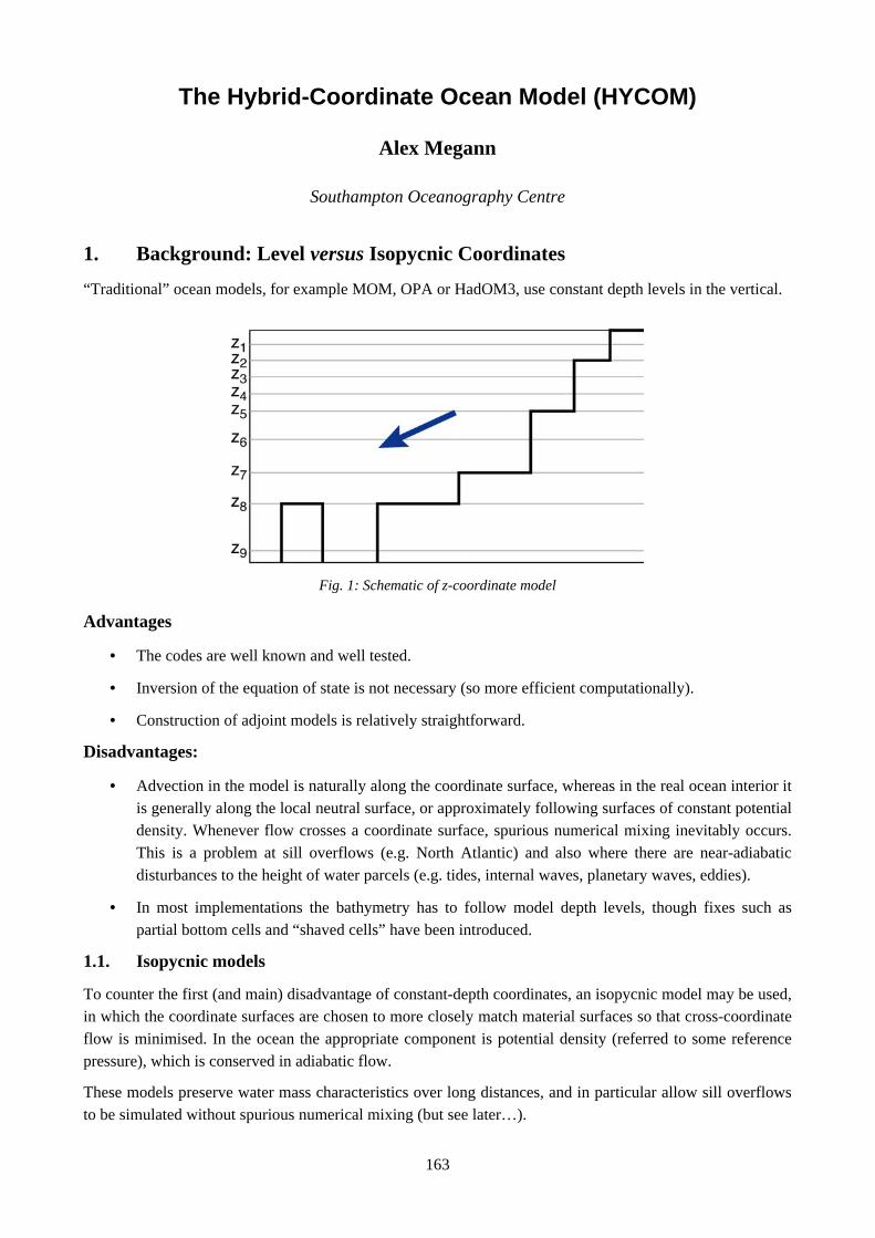
“Traditional” ocean models, for example MOM, OPA or HadOM3, use constant depth levels in the vertical.
Fig. 1: Schematic of z-coordinate model
Advantages
• The codes are well known and well tested.
• Inversion of the equation of state is not necessary (so more efficient computationally).
• Construction of adjoint models is relatively straightforward.
Disadvantages:
• Advection in the model is naturally along the coordinate surface, whereas in the real ocean interior it is generally along the local neutral surface, or approximately following surfaces of constant potential density. Whenever flow crosses a coordinate surface, spurious numerical mixing inevitably occurs. This is a problem at sill overflows (e.g. North Atlantic) and also where there are near-adiabatic disturbances to the height of water parcels (e.g. tides, internal waves, planetary waves, eddies).
• In most implementations the bathymetry has to follow model depth levels, though fixes such as partial bottom cells and “shaved cells” have been introduced.
1.1. Isopycnic models
To counter the first (and main) disadvantage of constant-depth coordinates, an isopycnic model may be used, in which the coordinate surfaces are chosen to more closely match material surfaces so that cross-coordinate flow is minimised. In the ocean the appropriate component is potential density (referred to some reference pressure), which is conserved in adiabatic flow.
These models preserve water mass characteristics over long distances, and in particular allow sill overflows to be simulated without spurious numerical mixing (but see later…).
163
MEGANN, A.: THE HYBRID-COORDINATE OCEAN MODEL (HYCOM)
2. The Miami Isopycnic Coordinate Ocean Model (MICOM)
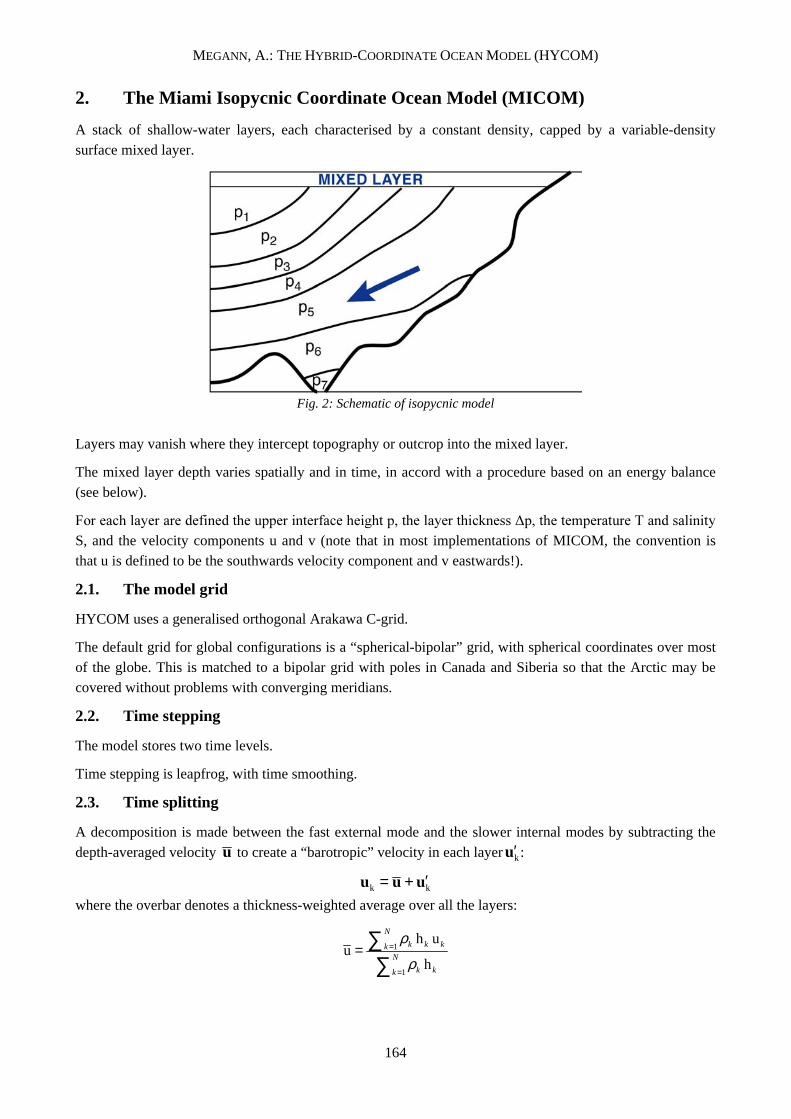
A stack of shallow-water layers, each characterised by a constant density, capped by a variable-density surface mixed layer.
Fig. 2: Schematic of isopycnic model
Layers may vanish where they intercept topography or outcrop into the mixed layer.
The mixed layer depth varies spatially and in time, in accord with a procedure based on an energy balance (see below).
S, and the velocity components u and v (note that in most implementations of MICOM, the convention is that u is defined to be the southwards velocity component and v eastwards!).
2.1. The model grid
HYCOM uses a generalised orthogonal Arakawa C-grid.
The default grid for global configurations is a “spherical-bipolar” grid, with spherical coordinates over most of the globe. This is matched to a bipolar grid with poles in Canada and Siberia so that the Arctic may be covered without problems with converging meridians.
2.2. Time stepping
The model stores two time levels.
Time stepping is leapfrog, with time smoothing.
2.3. Time splitting
A decomposition is made between the fast external mode and the slower internal modes by subtracting the depth-averaged velocity u to create a “barotropic” velocity in each layer ′ u k :
uk = u + ′ u k
where the overbar denotes a thickness-weighted average over all the layers:
1
1
h uu
h
N
k k kkN
k kk
ρ
ρ=
=
= ∑∑
164
MEGANN, A.: THE HYBRID-COORDINATE OCEAN MODEL (HYCOM)
The momentum equations for the “internal” and “external” modes are then solved separately: the latter has the same time step as that for the continuity equation and the thermodynamics, while the “barotropic” equation is solved with a shorter time step (normally 30-40 per “baroclinic” time step).
Note that this mode splitting is not exact, since the real fast mode is not entirely contained within the depth-integrated velocity. In fact theory predicts that this splitting is numerically unstable, but this does not seem to lead to problems in practice.
The advantage of this scheme is that it only requires summation in the vertical, and is horizontally local. It therefore scales trivially on a multiprocessor computing platform, unlike most z-coordinate models where a Poisson solver is required to solve for the free surface height.
We define the baroclinic velocity ku′ in terms of the depth-averaged velocity:
k ku u+ u′=
We define a rescaled layer thickness for the kth layer
( )k kp = 1+ pη ′∆ ∆
where ∆p is the pressure difference between top and bottom of the layer, H is the water depth and ηH is the surface elevation.
The rescaled bottom pressure bp′ is then given by the hydrostatic relation:
bp g Hρ′ =
where ρ is the mean density.
2.4. The continuity equation
This ensures the conservation of mass on model layers: the layer thickness responds to the divergence of the mass flux field, dilating or contracting each layer as necessary.
The basic equation solved is
( ) ( )kk bk
b
pp p p
t p
′∆∂ ′ ′∆ + ∇ ⋅ ∆ = ∇ ⋅ ∇′∂
u u
and this is done using the flux-corrected transport scheme of Zalesak (1986)
2.5. Interface depth diffusion
This is a parameterisation of the baroclinic instability process, where the available potential energy in sloping density surfaces is converted into kinetic energy on the scale of the Rossby radius. The interface depths pk are subject to a harmonic diffusion of the form
( ) k kp pν′ ′= ∇ ⋅ ∇�
It is similar to the Gent & McWilliams formulation (Gent & McWilliams, 1990), which parameterises diffusion according to the horizontal gradient of the vertical density gradient.
This parameterisation also contributes a term to the advective fluxes used for tracers: it there constitutes the “bolus” flux, representing the effect of baroclinic eddies on tracer transport.
2.6. Tracer advection and diffusion
The tendency equation for layer temperature in isopycnal coordinates is
165
MEGANN, A.: THE HYBRID-COORDINATE OCEAN MODEL (HYCOM)
( ) ( ) ( )bottom top
p pT p T p s T s T p T Q
t s sν∂ ∂ ∂ ∆ = ∇ ⋅ ∆ + − = ∇ ⋅ ∆ ∇ + ∂ ∂ ∂
u � �
Tracer advection is handled by the MPDATA scheme of Smolarkiewicz and Grabowski (1990), which ensures that advection cannot produce new extrema in the tracer fields, and also preserves the positive definite nature of the salinity field.
In MICOM the temperature and salinity on internal layers are constrained by the requirement that the density be identical to the layer density. This means that we have two choices:
• Advect salinity and diagnose temperature by inverting the equation of state.
• Advect temperature and diagnose salinity.
The usual choice is the first, chiefly because the equation of state is more nearly linear in salinity. The analytic equations of state used in ocean models (for example MICOM uses Friedrichs-Levitus) have a turning point in temperature at a few degrees below zero, so its inversion for T is not single-valued.
(T)du
(T)xv (T)
yv ( ) ( )uT Tx d x∆ = ∆
( ) ( )uT Ty d y∆ = ∆
( )2
2
uf M g
t p
τζ ∂ ∂+ ∇ + + × = −∇ − ∂ ∂
uk u
( )2 *
k kk
u uv -
2k b
k k k
u pf v M g
t x t p
η τζ ζρ
′ ′′ ∂ ∂∂ ∂+ ∇ + + = − − − − ∂ ∂ ∂ ∂
Fig. 3: Friedrich-Levitus equation of state for �0
The isopycnal diffusion of tracers is prescribed by a diffusion velocity from which the harmonic
diffusivity in the x and y directions and are calculated according to and
This formulation enhances the viscosity with the flow deformation, but reverts to a background value ud���
where there is no shear.
2.8. Solution of the barotropic model
The depth-averaged continuity equation is
( )1 0bb
pp
t
η η′∂ ′+ ∇ + = ∂
u
( )*u 1 u
fv bpt x t
ηρ
∂ ∂ ∂′− + = ∂ ∂ ∂
( )*1
b
v vfu p
t y tη
ρ∂ ∂ ∂′+ + = ∂ ∂ ∂
1/ 2
k
Ng
kz
κ
ρρ
−
=
∂= ∂
νu = max ud∆x,λ ∂u
∂x− ∂v
∂y
+
∂v
∂x+ ∂u
∂y
2
1
2
∆x2
where pb� ������'��������������������(� ������������������� ���
The equations of motion for the depth-averaged velocity are
and
where u*, v* are “pseudo-velocity” components already defined.
2.9. Diapycnal diffusion
The advection and diffusion algorithms in MICOM have intrinsically zero internal diapycnal diffusion.
The physical diapycnal diffusion of tracers is simulated by a mixing of T & S between layers with a diffusivity inversely proportional to the buoyancy frequency N:
where N is the buoyancy frequency in s-1. Normally a k of around 0.5 x 10⁻³ is used, which gives )�*�$��2/s in the ocean interior and 0.1 m2/s in the thermocline.
In MICOM there is no diapycnal diffusion of momentum (in other words, no viscosity between layers).
There is also no representation of entrainment of dense gravity flows (needed to accurately simulate sill overflows).
2.10. The mixed layer
MICOM uses one or other of the variants of the Kraus-Turner mixed layer model.
167
MEGANN, A.: THE HYBRID-COORDINATE OCEAN MODEL (HYCOM)
This is a bulk mixed layer model, where the surface layer is vertically entirely mixed, and whose base is a coordinate surface.
The salinity and temperature of the surface layer are changed in accord with applied surface fluxes, and then the mixed layer depth updated in accord with the balance between the potential energy associated with a the stability of the new stratification and the turbulent kinetic energy flux.
3. Hybrid Coordinates
3.1. Weaknesses of the pure isopycnic formulation
Although the isopycnic model has significant advantages in simulating large-scale interior flows in the ocean, it has several drawbacks, which can be critical in some applications:
• The detrainment of water from the mixed layer, with its continuously variable density, into the underlying layer, in which the density is fixed, is problematic.
• Parameterisation of entrainment by overflows is difficult,
• In regions with weak stratification, such as the Arctic the vertical resolution is poor, and
• In the above regimes, many of the model layers are massless, and so are wasted.
3.2. The Hybrid-Coordinate Ocean Model (HYCOM)
This was introduced by Rainer Bleck in the late 1990s, but followed ideas first implemented in atmospheric models but also tentatively used in an ocean model by Bleck and Boudra much earlier (1981).
The generalised vertical coordinate adjustment algorithm implemented in HYCOM is designed so that the isopycnic vertical coordinates present in the ocean interior transition smoothly to z coordinates in near-surface, well mixed regions, to sigma (terrain-following) coordinates in shallow water regions, and back to level coordinates in very shallow water to prevent layers from becoming very thin.
Fig. 4: schematic of isopycnic model
3.3. The regridding scheme
If the density of a given layer does not equal the isopycnic reference density, the interfaces bounding the layer are adjusted to return the density to its reference value.
For more details, see the handout “Generalised coordinate treatment in HYCOM” This also available from the HYCOM website: ftp://hycom.rsmas.miami.edu/bleck/hycom/hybrid.ps
MEGANN, A.: THE HYBRID-COORDINATE OCEAN MODEL (HYCOM)
The remapping process adjusts the upper or lower interface of a given layer in such a way as to restore its
potential density towards a target ρk. The algorithm differs depending on whether the density is larger or smaller than the target density.
In the deep ocean, the isopycnic-level coordinate transition is performed as follows
• If the layer is too light, the interface below is moved downward so that the entrained denser water returns the density to its reference value
• If the layer is too dense, the interface above is moved upward in the same manner
• If minimum coordinate separation is violated near the ocean surface, the cushion function is used to re-calculate the vertical coordinate location, prohibiting the restoration of isopycnic conditions.
• Two of the thermodynamic variables T, S, and density are mixed across the moving interfaces (user selectable), with the third calculated from the equation of state. If T and S are mixed, exact isopycnal density is not restored, but repeated application keeps the error small.
Fig. 5. CHIME coupled model: Temperature section in September in the North Pacific at 180°E. Layer interfaces are shown in black; mixed layer depth is shown by thick line. The transition can be seen from entirely isopycnic layers on the Equator (where there are watermasses present with the lightest densities) to the very north of the Pacific, where many constant-depth levels are deployed. The transition between constant-depth and terrain-following coordinates can also be seen on the continental shelf at the northern end of the section.
The user selects an absolute minimum thickness δ0. The function ∆0 is then selected to ensure a smooth
transition between isopycnic and non-isopycnic conditions for any layer, and is determined by a continuously differentiable “cushion” function, which for large positive arguments returns the
argument ∆p, and for large negative arguments returns δ0:
∆p ≡ ˆ p 1 −p0
∆ 0 = δ0 1+ ∆p3∆ 0
+ ∆p3∆ 0( )2
∆p ≤ 3δ0
∆p ∆p > 3δ0
The regridding is in practice a first-order upstream advection scheme so is fundamentally diffusive.
For this reason we want to minimise the amount of regridding performed by the model - otherwise we lose the main advantage of using density coordinates.
169
MEGANN, A.: THE HYBRID-COORDINATE OCEAN MODEL (HYCOM)
3.4. Diapycnal mixing schemes
An important difference between MICOM and HYCOM is that in the former the surface layer is identical to the mixed layer (and also the Ekman layer). In the latter by contrast the surface layer has no special role, except as a boundary layer through which all the surface fluxes are exchanged with the atmosphere (except for the fraction of downwelling visible radiation which penetrates to subsurface layers). In HYCOM the “mixed layer” over which surface buoyancy forcing and wind stress may mix tracers and momentum extends in the general case over several model layers.
The Kraus-Turner-type bulk mixed layer has been used with HYCOM but has drawbacks in this environment, which it shares with depth-coordinate models using a bulk mixed layer. In these cases the mixed layer depth is constrained to lie on a coordinate surface even when the Monin-Obukhov theory places it within a layer, and this leads to a noisy prognosed mixed-layer depth in the model with a bias towards deeper mixing (the MLD necessarily extends to the bottom of any layer).
The default mixing scheme in HYCOM is the KPP scheme (Large et al., 1994). In this the contributions to the diffusivities for temperature, salt and momentum from various parameterised processes are evaluated, the corresponding fluxes at each interface calculated, and a matrix method is used to solve the diffusion equation for each field. This is applied over the entire water column,
3.4.1. Processes parameterised
The surface mixed layer is then merely a depth range over which the diffusivities are enhanced relative to internal values.
The contributions to the diffusivity are from:
• Surface boundary layer:
o Mechanical wind mixing
o Buoyancy flux forcing
o Convective overturning
o Non-local (counter-gradient) fluxes
• Diapycnal mixing in ocean interior
o Internal wave breaking,
o Instability due to resolved vertical shear (Richardson number instability), and
o Double diffusion.
The KPP algorithm can run at relatively low vertical resolution.
3.4.2. Mixing Procedure
• Apply surface thermodynamic and momentum flux forcing.
• Calculate K profiles for interior diapycnal mixing from surface to bottom
• Diagnose turbulent boundary layer thickness
• Diagnose minimum depth H where a bulk Richardson number exceeds critical value
• Turbulent boundary layer eddies can penetrate to depth H where the fluid becomes stable relative to local buoyancy and velocity
• Calculate surface boundary layer k profiles for T, S, and momentum
• Vertical diffusivity for T and S are parameterized independently
170
MEGANN, A.: THE HYBRID-COORDINATE OCEAN MODEL (HYCOM)
• Choose coefficients to match the interior and boundary layer K profiles, producing a final K profile with a continuous first vertical derivative
• Solve diffusion equation semi-implicitly with two temporal iterations
• Diagnose mixed layer thickness along with T, S, u, and v
4. Interesting issues with isopycnic and hybrid coordinate models
4.1. Choice of reference pressure
Early implementations of MICOM used the ocean surface as reference pressure for the potential density (σ0
or σθ). This coordinate has the drawback of non-monotonicity in the deep Atlantic, so that North Atlantic
Deep Water (NADW) has a higher σ0 than Antarctic Bottom Water, even though the in situ density of
AABW is higher than that of NADW and therefore lies underneath the latter. These models cannot represent AABW.
Fig. 6. Potential density (σ0) at 30°W (September; Levitus 1992)
Fig. 7. Potential density inversions in the Atlantic with three different reference pressures: 0dbar (left), 2000 dbar (centre) and 4000 dbar (right), from Read, 1994.
171
MEGANN, A.: THE HYBRID-COORDINATE OCEAN MODEL (HYCOM)
More recent basin-scale and global versions of MICOM and indeed HYCOM use a reference pressure of 2000 dbar (~2000 metres), which is monotonic over most of the ocean (see Fig. 7).
4.2. Thermobaric correction
The compressibility of sea water is a function of temperature: cold water is more compressible than warm water. This has two main consequences:
• There is an error in the pressure gradient in an isopycnic layer where there is a strong temperature gradient along the layer. This is a significant problem in regions such as the Mediterranean salt tongue in the North Atlantic.
• Extremely cold water, such as the shelf water in the Weddell Sea, becomes more dense relative to the surrounding water as it flows off the shelf edge and sinks. This is one of the steps in the formation of Antarctic Bottom Water.
Sun et al. (1990) introduced a correction to the pressure gradient which accounts for the thermobaric effect to first order. This was found to give a more realistic Atlantic subpolar gyre circulation: without the correction the circulation was too strong.
Fig. 8. Thermal wind errors arising from using isopycnal slope. Shaded contours: salinity (interval 0.1 PSU) from Levitus (1994) climatology Hollow arrows: geostrophic velocity shear on σ0=27.83. Solid arrows: corrections to this estimate based on slope of σ0 surface to local neutral surface. From S. Sun, Ph.D Thesis.
4.3. Choice of upper ocean layer thicknesses
The choice of the minimum layer thickness ∆0 for each of the layers is non-trivial, as it determines
• The vertical resolution in the upper ocean, and hence the stratification and shear profiles, and
• The depth of the transition from isopycnic to non-isopycnic regimes.
The latter consequence is arguably more critical, as it affects the annual cycle of entrainment/detrainment, as well as the magnitude of any spurious diapycnal diffusion arising from non-isopycnal advection.
172
MEGANN, A.: THE HYBRID-COORDINATE OCEAN MODEL (HYCOM)
As a general rule we aim top place z-levels as much as possible within seasonal mixed layer.
HYCOM implementations usually use thin (~5m) minimum thickness close to the surface, increasing to 20m or so by 100m depth. In certain circumstances shallow surface lay can lead to unphysical upwelling (for reasons so far unknown).
4.4. Cabbeling and conservation
In a pure isopycnic model we have the constraint that the potential density in each layer is conserved – in other words if we vary S, T is determined. In MICOM salinity is advected and diffused, and then T is calculated by inverting the equation of state . This does not require any regridding in the
vertical, so generates zero diapycnal mixing. However, because the equation of state is non-linear, diffusion of water with different salinity within an isopycnal layer does not conserve potential temperature, so leads to an unphysical warming (cabbeling cannot occur).
T = T(ρk,S)
In the hybrid case we have more than one choice of variables to be advected and diffused: the advantages and disadvantages are different for each combination.
Advect and diffuse temperature and salinity
• Most physical choice - should conserve T & S and permits cabbeling
Advect and diffuse density and salinity (as in MICOM)
• Minimises diapycnal diffusion
• Cabbeling is not represented: result is internal warming
Advect density & salinity, but diffuse temperature & salinity
• Low diapycnal diffusion; represents cabbeling.
• Conservation properties are not well defined.
Some optimal combination of (B) and (C)
• Adjust weighting to empirically optimise global conservation properties
• Any combination is an arbitrary and empirical choice, and may not be appropriate locally; this conceals a fundamental (if slight in practice) problem with the model.
4.5. “Flexy” layers
An “Achilles heel” of constant-depth coordinates is that any vertical motion of isopycnal surfaces leads to mixing.
This is clearly also a problem in the surface layers of the hybrid model, where tides and internal waves will cause numerical mixing, even where the waves are themselves nearly adiabatic.
In HYCOM there is a way a way to minimise spurious mixing. Instead of imposing a rigid minimum �� ��������+0 at each time step, we can restore the thickness to the target thickness with a time scale of a day or two – in this way waves with a shorter period than this can pass through without mixing, while the layers are permitted to migrate vertically on seasonal timescales.
173
MEGANN, A.: THE HYBRID-COORDINATE OCEAN MODEL (HYCOM)
5. HYCOM Applications
Atlantic ocean-only simulations (RSMAS, Miami: Chassignet et al.)
High (1/12°) resolution to investigate the effect of the choice of vertical coordinate, reference pressure and of the thermobaric correction.
Pacific ocean-only simulations (NRL, Stennis: Metzger et al.)
http://hycom.rsmas.miami.edu/internal/seven/HYCOM-Metzger.pdf Again at 1/12°) resolution with surface fluxes, these are so far the state-of the art of HYCOM implementation, and show excellent realism.
CHIME (SOC: Megann and New)
Coupled model using the atmosphere and ice models from HadCM3, but with a 1.25° HYCOM as the ocean component. So far run for 120 years under a COAPEC funded project.
GISS coupled model (NASA GISS: Sun and Bleck)
Run with slightly lower resolution than CHIME. Has been used in greenhouse forcing experiments
Regional simulations (RSMAS and NRL, Stennis)
High-resolution studies of the Gulf of Mexico and around Japan.
Regional, global and coupled simulations (Bergen: Drange et al.)
Studies of the Arctic, Nordic and global domains
6. So… Does it work?
MICOM, a pure isopycnic model, is a conceptually simple tool which simulates flow on potential density surfaces. HYCOM offers the potential to combine the advantages of both z-coordinate and isopycnic models, but is still a relatively untested tool. There are many “knobs” whose optimum settings are still unknown. However, there are already very promising indications…
6.1. The equatorial thermocline
Z-coordinate models tend to have an unrealistically diffuse equatorial thermocline, since the flow in the latter follows a sloping density surface.
Fig. 9(a). Temperature cross-section at 135°W from CTD/ADCP data (Johnson and McPhaden, 2001
MEGANN, A.: THE HYBRID-COORDINATE OCEAN MODEL (HYCOM)
Fig. 9(b). Temperature cross-section at 135°W from 1/12° Pacific HYCOM
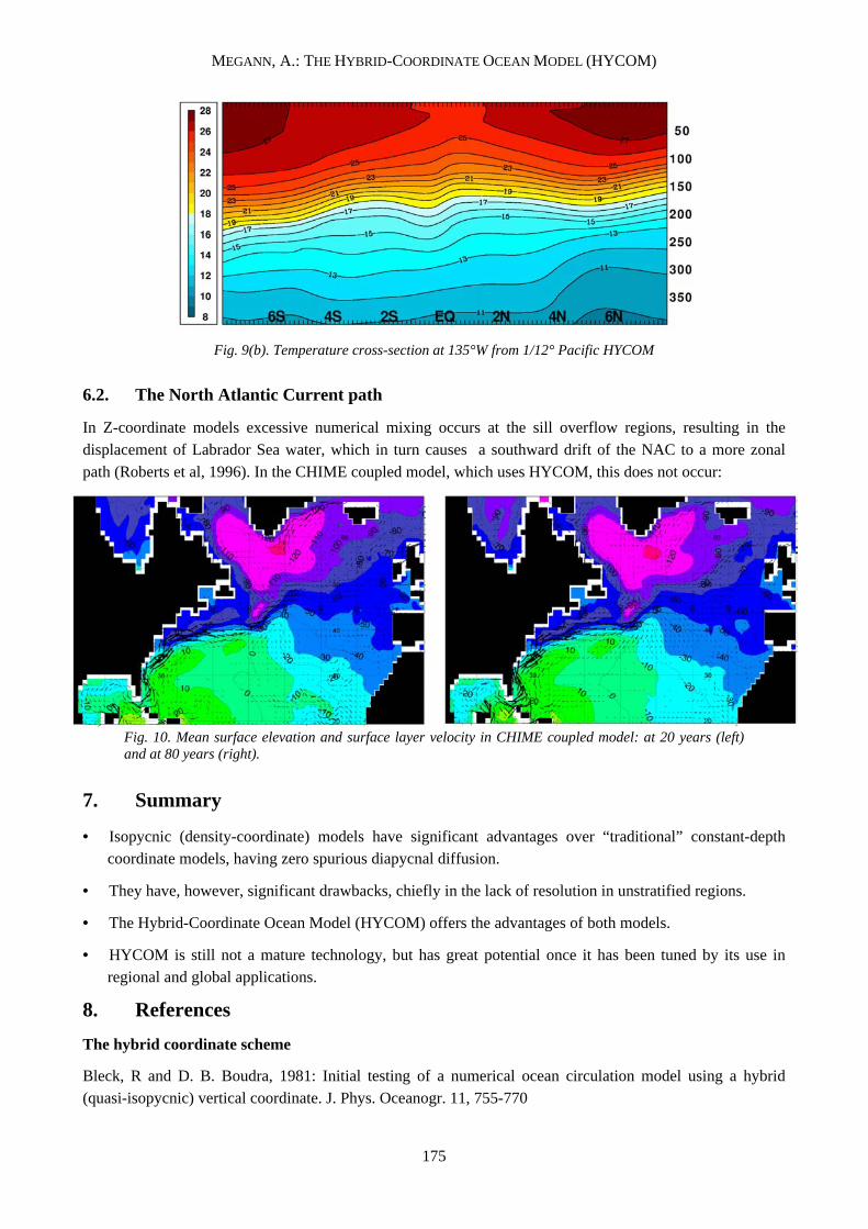
6.2. The North Atlantic Current path
In Z-coordinate models excessive numerical mixing occurs at the sill overflow regions, resulting in the displacement of Labrador Sea water, which in turn causes a southward drift of the NAC to a more zonal path (Roberts et al, 1996). In the CHIME coupled model, which uses HYCOM, this does not occur:
Fig. 10. Mean surface elevation and surface layer velocity in CHIME coupled model: at 20 years (left) and at 80 years (right).
7. Summary
• Isopycnic (density-coordinate) models have significant advantages over “traditional” constant-depth coordinate models, having zero spurious diapycnal diffusion.
• They have, however, significant drawbacks, chiefly in the lack of resolution in unstratified regions.
• The Hybrid-Coordinate Ocean Model (HYCOM) offers the advantages of both models.
• HYCOM is still not a mature technology, but has great potential once it has been tuned by its use in regional and global applications.
8. References
The hybrid coordinate scheme
Bleck, R and D. B. Boudra, 1981: Initial testing of a numerical ocean circulation model using a hybrid (quasi-isopycnic) vertical coordinate. J. Phys. Oceanogr. 11, 755-770
175
MEGANN, A.: THE HYBRID-COORDINATE OCEAN MODEL (HYCOM)
176
Bleck, R. and S. G. Benjamin, 1993. Regional weather prediction with a model combining terrain-following and isentropic coordinates. Part 1: model description. Monthly Weather Review 121, 1770-1785
Bleck, R., 2002: An oceanic general circulation model framed in hybrid isopycnic-cartesian coordinates, Ocean Modelling, B, 55-88.
Comparison of z-coordinate and isopycnic models in the North Atlantic:
Roberts, M.J., R. Marsh, A.L. New and R.A. Wood, 1996. An intercomparison of a Bryan-Cox-type ocean model and an isopycnic ocean model. Part I: the subpolar gyre and high-latitude processes. J. Phys. Oceanog. 26, 1495-1527.
The viscosity formulation used in MICOM & HYCOM:
Smagorinsky, J. (1963). General circulation experiments with the primitive equations: part I, the basic experiment. Monthly Weather Review, 91, 99--164.
Thermobaric correction:
Sun, S., R. Bleck, C. G. H. Rooth, J. Dukowicz, E. P. Chassignet, and P. Killworth, 1999: Inclusion of thermobaricity in isopycnic-coordinate ocean models. J. Phys. Oceanogr., 29, 2719-2729.
The Gent & McWilliams mixing scheme:
Gent, P. R. and J. C. McWilliams. 1990. Isopycnal mixing in ocean circulation models. J. Phys. Oceanog., 20, 150-155.
For a full description of the HYCOM code see the HYCOM manual, downloadable from http://oceanmodeling.rsmas.miami.edu/hycom/doc/hycom_users_manual.pdf (as is other interesting material on HYCOM)