77
Yngvi Bj ¨ ornsson Michael Thielscher (Eds.) The IJCAI-13 Workshop on General Game Playing General Intelligence in Game-Playing Agents, GIGA’13 Beijing, China, August 2013 Proceedings
Yngvi BjornssonMichael Thielscher (Eds.)
The IJCAI-13 Workshop onGeneral Game Playing
General Intelligence in Game-Playing Agents, GIGA’13
Beijing, China, August 2013Proceedings

GIGA'13 Proceedings2
Preface
Artificial Intelligence (AI) researchers have for decades worked on building game-playing agents capable of match-ing wits with the strongest humans in the world, resulting in several success stories for games like chess and checkers.The success of such systems has been partly due to years of relentless knowledge-engineering effort on behalf of theprogram developers, manually adding application-dependent knowledge to their game-playing agents. The variousalgorithmic enhancements used are often highly tailored towards the game at hand.
Research into general game playing (GGP) aims at taking this approach to the next level: to build intelligent softwareagents that can, given the rules of any game, automatically learn a strategy for playing that game at an expert levelwithout any human intervention. In contrast to software systems designed to play one specific game, systems capableof playing arbitrary unseen games cannot be provided with game-specific domain knowledge a priori. Instead, theymust be endowed with high-level abilities to learn strategies and perform abstract reasoning. Successful realizationof such programs poses many interesting research challenges for a wide variety of artificial-intelligence sub-areasincluding (but not limited to):
• knowledge representation and reasoning,• heuristic search and automated planning,• computational game-theory,• multi-agent systems,• machine learning,• game playing and design,• artificial general intelligence,• opponent modeling,• evaluation and analysis.
These are the proceedings of GIGA’13, the third ever workshop on General Intelligence in Game-Playing Agentsfollowing the inaugural GIGA Workshop at IJCAI’09 in Pasadena (USA) and the follow-up event at IJCAI’11 inBarcelona (Spain). This workshop series has been established to become the major forum for discussing, presentingand promoting research on General Game Playing. It is intended to bring together researchers from the abovesub-fields of AI to discuss how best to address the challenges and further advance the state-of-the-art of generalgame-playing systems and generic artificial intelligence.
These proceedings contain the 9 papers that have been selected for presentation at this workshop. All submissionswere reviewed by a distinguished international program committee. The accepted papers cover a multitude of topicssuch as the fast inference for game descriptions, advanced simulation-based methods, general imperfect-informationgame playing, and automated reasoning about games.
For the first time ever, GIGA’13 proudly presents the award for the Best Student-Only Paper, which comes with afree registration for the presenting author. We congratulate Michael Schofield and Abdallah Saffidine on winningthis inaugural award with their contribution entitled “High Speed Forward Chaining for General Game Playing.”
We thank all the authors for responding to the call for papers with their high quality submissions, and the programcommittee members and other reviewers for their valuable feedback and comments. We also thank IJCAI for alltheir help and support.
We welcome all our delegates and hope that all will enjoy the workshop and through it find inspiration for continuingtheir work on the many facets of General Game Playing!
August 2013 Yngvi BjornssonMichael Thielscher
GIGA'13 Proceedings 3

Organization
Workshop Chairs
Yngvi Bjornsson, Reykjavık University, IcelandMichael Thielscher, The University of New South Wales, Australia
Program Committee
Yngvi Bjornsson Reykjavık UniversityTristan Cazenave Universite Paris-DauphineStefan Edelkamp University of Bremen
Hilmar Finnsson Reykjavık UniversityMichael Genesereth Stanford UniversityLukasz Kaiser Universite Paris Diderot
Gregory Kuhlmann Apple Inc.Abdallah Saffidine Universite Paris-Dauphine
Marius Schneider University of PotsdamStephan Schiffel Reykjavık University
Sam Schreiber Google Inc.Nathan Sturtevant University of Denver
Mark Winands Maastricht University
Additional Reviewer
Michael Schofield
GIGA'13 Proceedings4
Table of Contents
A Legal Player for GDL-II Based on Filtering With Logic Programs . . . . . . . . . . . . . . . . . . . . . . . . . . . . . . . . . . . . . . . . 7Michael Thielscher
Sufficiency-Based Selection Strategy for MCTS . . . . . . . . . . . . . . . . . . . . . . . . . . . . . . . . . . . . . . . . . . . . . . . . . . . . . . . . . 15Stefan Freyr Gudmundsson, Yngvi Bjornsson
Decaying Simulation Strategies . . . . . . . . . . . . . . . . . . . . . . . . . . . . . . . . . . . . . . . . . . . . . . . . . . . . . . . . . . . . . . . . . . . . . . . . 23M.J.W. Tak, Mark H. M. Winands, Yngvi Bjornsson
High Speed Forward Chaining for General Game Playing . . . . . . . . . . . . . . . . . . . . . . . . . . . . . . . . . . . . . . . . . . . . . . . . . 31Michael Schofield, Abdallah Saffidine
Lifting HyperPlay for General Game Playing to Incomplete-Information Models . . . . . . . . . . . . . . . . . . . . . . . . . . . . 39Michael Schofield, Timothy Cerexhe, Michael Thielscher
Model Checking for Reasoning About Incomplete Information Games . . . . . . . . . . . . . . . . . . . . . . . . . . . . . . . . . . . . . 47Xiaowei Huang, Ji Ruan, Michael Thielscher
Comparison of GDL Reasoners . . . . . . . . . . . . . . . . . . . . . . . . . . . . . . . . . . . . . . . . . . . . . . . . . . . . . . . . . . . . . . . . . . . . . . . . 55Yngvi Bjornsson, Stephan Schiffel
Online Adjustment of Tree Search for GGP . . . . . . . . . . . . . . . . . . . . . . . . . . . . . . . . . . . . . . . . . . . . . . . . . . . . . . . . . . . . . . 63Jean Mehat, Jean Noel Vittaut
Stratified Logic Program Updates for General Game-Playing . . . . . . . . . . . . . . . . . . . . . . . . . . . . . . . . . . . . . . . . . . . . . . 71David Spies
GIGA'13 Proceedings 5

GIGA'13 Proceedings6
A Legal Player for GDL-II Based on Filtering With Logic Programs∗
Michael ThielscherSchool of Computer Science and Engineering
University of New South WalesAustralia
AbstractMotivated by the problem of build-ing a basic reasoner for general gameplaying with imperfect information, weaddress the problem of filtering withlogic programs, whereby an agent up-dates its incomplete knowledge of aprogram by observations. We developa filtering method by adapting an ex-isting backward-chaining and abduc-tion method for so-called open logicprograms. Experimental results showthat this provides a basic effectiveand efficient “legal” player for generalimperfect-information games.
IntroductionA general game-playing (GGP) system is one that can un-derstand the rules of arbitrary games and use these rules toplay effectively. The annual GGP competition at AAAI hasbeen established in 2005 to foster research in this area [Gene-sereth et al., 2005]. While the competition in the past has fo-cused on games in which players always know the completegame state, a recent extension [Thielscher, 2011] of the for-mal game description language GDL also allows the descrip-tion of general randomized games with imperfect and asym-metric information [Quenault and Cazenave, 2007].
GDL uses normal logic program clauses to describe therules of a game [Genesereth et al., 2005]. For games withperfect information, standard resolution techniques can beused to build a basic, so-called legal player that throughouta game always knows its allowed moves [Love et al., 2006].Efficient variations exist that use tailored data structures andalgorithms for computing moves in classic GDL [Schkufzaet al., 2008; Waugh, 2009; Kissmann and Edelkamp, 2010;Saffidine and Cazenave, 2011]. But the generalization toimperfect-information games raises a fundamentally new rea-soning challenge even for such a basic player. Comput-ing with all possible states is practically infeasible exceptfor very simple games [Parker et al., 2005]. This is why
∗This submission is a slightly extended version of a paper thathas been accepted for AAAI’13.
the only two existing GGP systems described in the litera-ture for imperfect-information GDL [Edelkamp et al., 2012;Schofield et al., 2012] use the more practical alternative ofrandomly sampling states [Richards and Amir, 2009; Silverand Veness, 2010]. But in so doing these players reason witha mere subset of all models, which is logically incorrect.
In this paper we address the problem of building a logi-cally sound and efficient basic reasoning system for generalimperfect-information games by first isolating and addressingthe problem of filtering with logic programs: Suppose given alogic program with some hidden facts of which we have onlypartial knowledge. Suppose further that some consequencesof this incomplete program can be observed. The questionthen is, what other conclusions can we derive from our lim-ited knowledge plus the observations? This can be seen asan instance of the general notion of filtering as any processby which an agent updates its belief according to observa-tions [Amir and Russell, 2003].
We develop a method for filtering with logic programs un-der the assumption that incomplete knowledge is representedby two sets containing, respectively, known and unknownatoms, in the sense of 3-valued logic [Kleene, 1952]. Adapt-ing an inference method for abduction in so-called open logicprograms [Bonatti, 2001a; 2001b], we show how a method forfiltering can be obtained by augmenting standard backward-chaining with the computation of support.
We apply this method for filtering with logic programsto build a legal player for general game playing with im-perfect information that, just like its counterpart for perfect-information games, is based on backward-chaining. We provethat the reasoner thus obtained is sound. We also show it tobe complete if, as in perfect-information games, the playercan observe all other players’ moves. Experimental resultswith all imperfect-information games used at past GGP com-petitions demonstrate the effectiveness and efficiency of ourmethod for a legal player to always know its allowed moves inalmost all games. This in fact supports an argument that canbe made for requiring that all games for competitions suchas at AAAI be written so that basic backward-chaining is allthat is needed to derive a player’s legal moves. Interestingly,the experiments also revealed that in many existing game de-scriptions players are not given enough information to knowthe outcome after termination.
After the following brief summary of GDL, we define the
GIGA'13 Proceedings 7
problem of filtering with logic programs. We then develop afiltering method based on backward-chaining and abductionof support. We apply this to build a basic and logically soundlegal player, present our experimental results, and conclude.
Background: GDL-IIThe science of general game playing requires a formal lan-guage for specifying arbitrary games by a complete set ofrules. The declarative Game Description Language (GDL)serves this purpose [Genesereth et al., 2005]. It uses the syn-tax of normal logic programs [Lloyd, 1987] and is character-ized by these special keywords:
role(R) R is a playerinit(F) feature F holds in the initial positiontrue(F) feature F holds in the current positionlegal(R,M) R has move M in the current positiondoes(R,M) player R does move Mnext(F) feature F holds in the next positionterminal the current position is terminalgoal(R,V) player R gets payoff Vdistinct(X,Y) terms X,Y are syntactically different
sees(R,P) player R is told P in the next positionrandom the random player (aka. Nature)
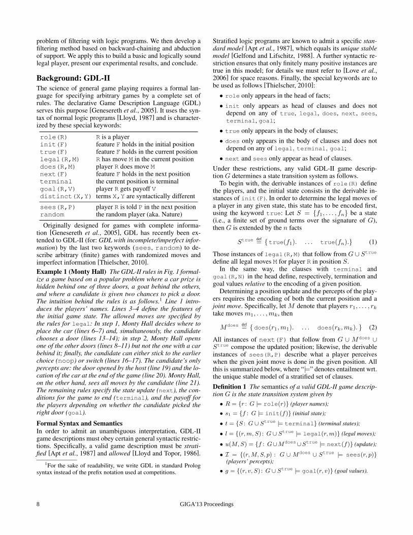
Originally designed for games with complete informa-tion [Genesereth et al., 2005], GDL has recently been ex-tended to GDL-II (for: GDL with incomplete/imperfect infor-mation) by the last two keywords (sees, random) to de-scribe arbitrary (finite) games with randomized moves andimperfect information [Thielscher, 2010].Example 1 (Monty Hall) The GDL-II rules in Fig. 1 formal-ize a game based on a popular problem where a car prize ishidden behind one of three doors, a goat behind the others,and where a candidate is given two chances to pick a door.The intuition behind the rules is as follows.1 Line 1 intro-duces the players’ names. Lines 3–4 define the features ofthe initial game state. The allowed moves are specified bythe rules for legal: In step 1, Monty Hall decides where toplace the car (lines 6–7) and, simultaneously, the candidatechooses a door (lines 13–14); in step 2, Monty Hall opensone of the other doors (lines 8–11) but not the one with a carbehind it; finally, the candidate can either stick to the earlierchoice (noop) or switch (lines 16–17). The candidate’s onlypercepts are: the door opened by the host (line 19) and the lo-cation of the car at the end of the game (line 20). Monty Hall,on the other hand, sees all moves by the candidate (line 21).The remaining rules specify the state update (next), the con-ditions for the game to end (terminal), and the payoff forthe players depending on whether the candidate picked theright door (goal).
Formal Syntax and SemanticsIn order to admit an unambiguous interpretation, GDL-IIgame descriptions must obey certain general syntactic restric-tions. Specifically, a valid game description must be strati-fied [Apt et al., 1987] and allowed [Lloyd and Topor, 1986].
1For the sake of readability, we write GDL in standard Prologsyntax instead of the prefix notation used at competitions.
Stratified logic programs are known to admit a specific stan-dard model [Apt et al., 1987], which equals its unique stablemodel [Gelfond and Lifschitz, 1988]. A further syntactic re-striction ensures that only finitely many positive instances aretrue in this model; for details we must refer to [Love et al.,2006] for space reasons. Finally, the special keywords are tobe used as follows [Thielscher, 2010]:
• role only appears in the head of facts;
• init only appears as head of clauses and does notdepend on any of true, legal, does, next, sees,terminal, goal;
• true only appears in the body of clauses;
• does only appears in the body of clauses and does notdepend on any of legal, terminal, goal;
• next and sees only appear as head of clauses.
Under these restrictions, any valid GDL-II game descrip-tion G determines a state transition system as follows.
To begin with, the derivable instances of role(R) definethe players, and the initial state consists in the derivable in-stances of init(F). In order to determine the legal moves ofa player in any given state, this state has to be encoded first,using the keyword true: Let S = f1, . . . , fn be a state(i.e., a finite set of ground terms over the signature of G),then G is extended by the n facts
Struedef= true(f1). . . . true(fn). (1)
Those instances of legal(R,M) that follow from G ∪ Struedefine all legal moves M for player R in position S.
In the same way, the clauses with terminal andgoal(R,N) in the head define, respectively, termination andgoal values relative to the encoding of a given position.
Determining a position update and the percepts of the play-ers requires the encoding of both the current position and ajoint move. Specifically, let M denote that players r1, . . . , rktake moves m1, . . . ,mk, then
Mdoes def= does(r1,m1). . . . does(rk,mk). (2)
All instances of next(F) that follow from G ∪ Mdoes ∪Strue compose the updated position; likewise, the derivableinstances of sees(R,P) describe what a player perceiveswhen the given joint move is done in the given position. Allthis is summarized below, where “|=” denotes entailment wrt.the unique stable model of a stratified set of clauses.
Definition 1 The semantics of a valid GDL-II game descrip-tion G is the state transition system given by• R = r : G |= role(r) (player names);
• s1 = f : G |= init(f) (initial state);
• t = S : G ∪ Strue |= terminal (terminal states);
• l = (r,m, S) : G ∪ Strue |= legal(r,m) (legal moves);
• u(M,S) = f : G∪Mdoes∪Strue |= next(f) (update);
• I = (r,M, S, p) : G ∪ Mdoes ∪ Strue |= sees(r, p)(players’ percepts);
• g = (r, v, S) : G ∪ Strue |= goal(r, v) (goal values).
GIGA'13 Proceedings8
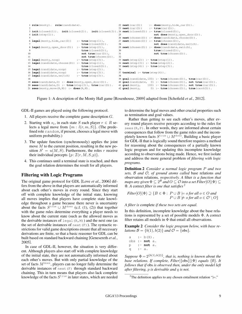
1 role(monty). role(candidate).23 init(closed(1)). init(closed(2)). init(closed(3)).4 init(step(1)).56 legal(monty,hide_car(D)) :- true(step(1)),7 true(closed(D)).8 legal(monty,open_door(D)) :- true(step(2)),9 true(closed(D)),
10 not true(car(D)),11 not true(chosen(D)).12 legal(monty,noop) :- true(step(3)).13 legal(candidate,choose(D)) :- true(step(1)),14 true(closed(D)).15 legal(candidate,noop) :- true(step(2)).16 legal(candidate,noop) :- true(step(3)).17 legal(candidate,switch) :- true(step(3)).1819 sees(candidate,D) :- does(monty,open_door(D)).20 sees(candidate,D) :- true(step(3)), true(car(D)).21 sees(monty,move(R,M)) :- does(R,M).
22 next(car(D)) :- does(monty,hide_car(D)).23 next(car(D)) :- true(car(D)).24 next(closed(D)) :- true(closed(D)),25 not does(monty,open_door(D)).26 next(chosen(D)) :- does(candidate,choose(D)).27 next(chosen(D)) :- true(chosen(D)),28 not does(candidate,switch).29 next(chosen(D)) :- does(candidate,switch),30 true(closed(D)),31 not true(chosen(D)).3233 next(step(2)) :- true(step(1)).34 next(step(3)) :- true(step(2)).35 next(step(4)) :- true(step(3)).3637 terminal :- true(step(4)).3839 goal(candidate,100) :- true(chosen(D)), true(car(D)).40 goal(candidate, 0) :- true(chosen(D)), not true(car(D)).41 goal(monty, 100) :- true(chosen(D)), not true(car(D)).42 goal(monty, 0) :- true(chosen(D)), true(card(D)).
Figure 1: A description of the Monty Hall game [Rosenhouse, 2009] adapted from [Schofield et al., 2012].
GDL-II games are played using the following protocol.
1. All players receive the complete game description G.
2. Starting with s1, in each state S each player r ∈ R se-lects a legal move from m : l(r,m, S). (The prede-fined role random, if present, chooses a legal move withuniform probability.)
3. The update function (synchronously) applies the jointmove M to the current position, resulting in the new po-sition S′ = u(M,S). Furthermore, the roles r receivetheir individual percepts p : I(r,M, S, p).
4. This continues until a terminal state is reached, and thenthe goal relation determines the result for all players.
Filtering with Logic ProgramsThe original game protocol for GDL [Love et al., 2006] dif-fers from the above in that players are automatically informedabout each other’s moves in every round. Since they startoff with complete knowledge of the initial state, knowingall moves implies that players have complete state knowl-edge throughout a game because there never is uncertaintyabout the facts Strue ∪ Mdoes (c.f. (1), (2)) that togetherwith the game rules determine everything a player needs toknow about the current state (such as the allowed moves asthe derivable instances of legal(R,M)) and the next one (asthe set of derivable instances of next(F)). The syntactic re-strictions for valid game descriptions ensure that all necessaryderivations are finite, so that a basic reasoner for GDL can bebuilt based on standard backward chaining [Genesereth et al.,2005].
In case of GDL-II, however, the situation is very differ-ent. Although players also start off with complete knowledgeof the initial state, they are not automatically informed abouteach other’s moves. But with only partial knowledge of theset of facts Mdoes, players can no longer fully determine thederivable instances of next(F) through standard backwardchaining. This in turn means that players also lack completeknowledge of the facts Strue in later states, which are needed
to determine the legal moves and other crucial properties suchas termination and goal values.
Rather than getting to see each other’s moves, after ev-ery round players receive percepts according to the rules forsees(R,P). In other words, they are informed about certainconsequences that follow from the game rules and the incom-pletely known facts Strue ∪Mdoes. Building a basic playerfor GDL-II that is logically sound therefore requires a methodfor reasoning about the consequences of a partially knownlogic program and for updating this incomplete knowledgeaccording to observations being made. Hence, we first isolateand address the more general problem of filtering with logicprograms.
Definition 2 Consider a normal logic program P and twosets, B and O, of ground atoms called base relations andobservation relations, respectively. A filter is a function thatmaps any given Φ ⊆ 2B andO ⊆ O into a set Filter[O](Φ) ⊆Φ. A correct filter is one that satisfies 2
Filter[O](Φ) ⊇ B ∈ Φ : P ∪B |= o for all o ∈ O andP ∪B 6|= o for all o ∈ O \O
A filter is complete if these two sets are equal.
In this definition, incomplete knowledge about the base rela-tions is represented by a set of possible models Φ. A correctfilter retains all models in Φ that entail all observations.
Example 2 Consider the logic program below, with base re-lations B = b(1), b(2) and O = obs.
a :- b(X).obs :- not a.p :- not a.q :- a.
Suppose Φ = 2b(1),b(2), that is, nothing is known about thebase relations. If complete, Filter[obs](Φ) equals ∅. Itfollows that if obs is observed then, under the only model leftafter filtering, p is derivable and q is not.
2The definition applies to any chosen entailment relation “|=.”
GIGA'13 Proceedings 9
Example 3 Consider the GDL in Fig. 1 with the instancesof true(F) and does(R,M) as base relations. Let Φ besuch that all of true(closed(1)), true(closed(2)),true(closed(3)), true(chosen(1)), true(step(1)),does(candidate,noop) are true in all models in Φ, and letO = sees(candidate,2),sees(candidate,3).
Suppose that we observe O = sees(candidate,3),then does(monty,open(3)) is true in all models result-ing from a complete filter (cf. line 19 in Fig. 1), whiledoes(monty,open(2)) is false in each of them. It follows,for instance, that in all models remaining after filtering,next(closed(1)) and next(closed(2)) are derivable butnot next(closed(3)) (cf. line 24–25).
A Basic Legal Player for GDL-IIIn this section we present a method for constructing a rea-soner for GDL-II based on a method for filtering that operateson a compact representation of incomplete information.
Representing Incomplete Information About FactsSince explicitly maintaining the set of possible states is prac-tically infeasible in most games, we base our approach to fil-tering on a coarser but practically feasible encoding usingtwo sets of ground atoms, B+ ⊆ B and B0 ⊆ B, whichrespectively contain the base relations that are known to betrue and those that may be true. Any such pair that satisfiesB+ ∩ B0 = ∅ implicitly represents the set of models
ΦB+,B0def= B+ ∪B : B ⊆ B0 (3)
This representation allows us to base our filtering method on aderivation mechanism that has been developed in the contextof so-called open logic programs [Bonatti, 2001a].
Reasoning with Open Logic ProgramsIn the following we adapt some basic definitions and resultsfrom [Bonatti, 2001a; 2001b] to our setting. Our open logicprograms are triples Ω = 〈P,B+,B0〉 where P is a normallogic program and B+,B0 are as above. A program P ′ iscalled an extension3 of Ω if P ′ = P ∪ B+ ∪ B for someB ⊆ B0. This gives rise to two modes of reasoning:
1. Skeptical inference: Ω |=s ϕ iff all stable models of allextensions P ′ of Ω entail ϕ.
2. Credulous inference: Ω |=c ϕ iff some stable model ofsome extension P ′ of Ω entails ϕ.
As observed in [Bonatti, 2001a], these two methods of infer-ence are dual to each other: Ω |=s ϕ iff Ω 6|=c notϕ andΩ |=c ϕ iff Ω 6|=s notϕ. We also make use of the followingconcepts [Bonatti, 2001b]:
1. A support for a ground atom A is a query Q obtained byunfolding A in P ∪ B+ until all the literals in Q eitheroccur in B0 or are negative.
2. A countersupport for a ground atomA is a set of groundliterals S such that each L ∈ S is the complement of
3This is called a completion in [Bonatti, 2001a], which howeverclashes with another concept so named earlier [Shepherdson, 1984].
some literal belonging to a support ofA; and conversely,each support of A contains a literal whose complementis in S.
In the following, for a set S of literals we denote by S+ theset of positive atoms in S and by S− the set of atoms thatoccur negated in S. A support is consistent iff S+ ∩ S− = ∅.
A Backward-Chaining Proof MethodThe definitions from above form the basis of a backward-chaining derivation procedure for computing answer substi-tutions θ along with supports for literals L wrt. an open pro-gram Ω = 〈P,B+,B0〉 using the following derivation rules.
1. If Lθ ∈ B+, return θ along with support ∅.2. If Lθ ∈ B0, return θ along with support Lθ.3. If L = ¬A is a negative ground literal and S the set of
computed supports for A, return the empty substitutionalong with a consistent set containing the complementof some literal from each element in S.
4. If L = A is positive and unifiable with the head of aclause from P , unfold A and return the union, if con-sistent, of supports for all literals in the resulting queryalong with the combined answer substitutions.
Recall, for instance, the short program from Example 2 andsuppose B+ = ∅ and B0 = b(1), b(2). Query b(X) admitstwo computed supports: S = b(1) with θ = X \ 1, andS = b(2) with θ = X \ 2. Hence, the computed coun-tersupport for query a is ¬b(1),¬b(2), which in turn is the(only) support for obs under the given sets B+,B0.
The above derivation rules are a subset of the calculus de-fined in [Bonatti, 2001a; 2001b] but constitute a complete anddecidable derivation procedure if the underlying logic pro-gram is syntactically restricted.Proposition 1 Let Ω = 〈P,B+,B0〉 be an open logic pro-gram with a finite Herbrand base and stratified program P .
1. Every computed support θ, S for a query Q satisfies〈P,B+ ∪ S+,B0 \ S−〉 |=s Qθ.
2. If 〈P,B+,B0〉 |=c Qτ for some τ , then there exists acomputed support θ, S forQ with θ more general than τ .
In the following, by Ω `θ,S A we denote that substitution θtogether with some S is a computed support for atom A wrt.open logic program Ω. In particular, Ω `θ,∅ A means that Aθfollows without additional support, i.e., is necessarily true inall extensions and hence skeptically entailed by Ω.
Filtering Based on Backward ChainingNext, we use the backward chaining-based method for openlogic programs to define a basic method for filtering withlogic programs. In the following, by Supp(Q) we denote theset of all computed supports for query Q. Consider a normallogic program P ; sets B+,B0; and a set O ⊆ O of obser-vations. We compute Filter[O](ΦB+,B0) as two sets B+new andB0new as follows.
B+new = B+ ∪
⋃o∈O
⋂S∈Supp(o)
S+ ∪⋃
o∈O\O
⋂S∈Supp(¬o)
S+
GIGA'13 Proceedings10

B0new = (B0\B+new)\
⋃o∈O
⋂S∈Supp(o)
S− ∪⋃
o∈O\O
⋂S∈Supp(¬o)
S−
Put in words, for each observation o made (resp. not made)we compute all supports (resp. all supports for ¬o) and then“strengthen” B+,B0 by every literal that is contained in allsupports. More precisely, if a literal occurs positively in everysupport for some o (resp. ¬o), then it is added to B+ andremoved from B0. Also removed from B0 are the literals thatoccur negatively in every support for some o (resp. ¬o).Example 4 Recall again the program from Example 2. Aswe have seen, when B+ = ∅ and B0 = b(1), b(2) thenthe query obs has one support, namely, ¬b(1),¬b(2). Thisyields B+new = ∅ and B0new = ∅. On the other hand, considerthe query ¬obs. It has two supports, b(1) and b(2). Theirintersection being empty implies B+new = B+ and B0new = B0,i.e., nothing new is learned by not seeing obs.
Proposition 2 Under the assumptions of Proposition 1, thefilter defined above is correct.
Proof: By Definition 2 we need to show that B ∈ ΦB+new,B0
newif B ∈ ΦB+,B0 and P ∪ B |= o for o ∈ O while P ∪B 6|= ofor o ∈ O \ O. So suppose the latter are all true, then foreach o ∈ O (and each o ∈ O \ O, resp.) there must be acomputed support S ∈ Supp(o) (resp., S ∈ Supp(¬o)) suchthat S+ ⊆ B and S− ∩B = ∅. By construction of B+new,B0newthis implies B+new ⊆ B ⊆ B+new∪B0
new. Hence,B ∈ ΦB+new,B0
newaccording to (3).
Since the compact representation of incomplete knowledgevia (3) does not support reasoning by disjunction, the fil-ter is necessarily incomplete. Recall, for instance, the sec-ond case in Example 4. Not observing obs means that b(1)or b(2) must be true. Hence, model ∅ could be filtered outbut is not because no two sets B+,B0 can encode Φ =b(1), b(2), b(1), b(2) via (3).
A Basic Update MethodThe method for filtering with logic programs forms the coreof our approach to building a basic reasoner for GDL-II. Thesyntactic restrictions for GDL-II ensure that the underlyingopen logic program satisfies the conditions Propositions 1and 2. This will guarantee that the knowledge the player keepsin B+,B0 is always correct.
The procedure for maintaining the player’s incompleteknowledge about a state is as follows, where G denotes theGDL-II description of a game whose semantics is given asper Definition 1; and where my role ∈ R is the role assignedto the player.
1. B+ :=true(F)θ : 〈G, ∅, ∅〉 `θ,∅ init(F); B0 := ∅2. In every round,
2.1 Compute the possible legal moves of all other roles:
L :=(R,M)θ : 〈G,B+,B0〉`θ,Slegal(R,M), R 6=my role
2.2 Let my move be the selected move of the basicplayer and my percepts the player’s percepts.– Let B+ := B+ ∪ does(my role,my move)
B0 := B0 ∪ does(R,M) : (R,M)∈ L
– Now, let
O := sees(my role,P)θ :〈G,B+,B0〉 `θ,S sees(my role,P)
O := sees(my role, p) : p ∈ my percepts
and compute B+new,B0new as the result of filteringB+,B0 by O wrt. G and O.
– The knowledge about the next state is obtainedas
B+ := true(F)θ : 〈G,B+new,B0new〉 `θ,∅ next(F)B0 := true(F)θ : 〈G,B+new,B0new〉 `θ,S next(F)\B+
3. The player knows that the game has terminated in case〈G,B+,B0〉 `ε,∅ terminal.
Put in words, the player starts with complete informationabout the initial state (step 1). In every round, the player’sknowledge is characterized by the skeptical consequences ofthe open logic program consisting of the game rules plus theincomplete knowledge B+,B0; specifically, this allows us todetermine the player’s own known legal moves as
Mθ : 〈G,B+,B0〉 `θ,∅ legal(my role,M)4
The incomplete knowledge also allows us to compute cred-ulous consequences, in particular the possible legal movesof all other players (step 2.1). For the update of B+,B0(step 2.2), we first add to B+ the knowledge of the player’sown move and to B0 the possible moves by the opponents.This allows us to determine the range of possible observa-tions, O, in order then to filter the player’s knowledge by ac-tual observations O. Finally, the player’s knowledge of theupdated state is determined as the skeptically (for B+) andcredulously (for B0) entailed instances of next(F).
The incompleteness of the filtering implies that the rea-soner for GDL-II thus defined is incomplete in general. It is,however, easy to show that it is complete in case the onlysees-rule for a player is
sees(player,move(R,M)) :- does(R,M).
This is so because under this rule the only support for an in-stance sees(player,move(r,m)) is does(r,m), and theonly countersupport in case the observation is not made is¬does(r,m). Hence, the filter will add the former to B+ andremove all of the latter from B0. The update procedure willthen result in complete knowledge whenever the player startswith complete knowledge.
Experimental ResultsBecause the representation of incomplete knowledge and thebackward chaining-based filtering are in themselves incom-plete, we have run experiments to test both the effectivenessand the efficiency of our method. We have used a simple im-plementation in the form of a vanilla meta-interpreter in Pro-log. We have run experiments with all games that were played
4The player knows that it doesn’t know all its legal moves if someinstance legal(my role,M) can be derived only with non-emptysupport, i.e., is credulously but not skeptically entailed.
GIGA'13 Proceedings 11
Game Legal Terminal Goal TimeBackgammon X X X 8.84Banker/Thief (role 1) X X no 0.42Banker/Thief (role 2) X X no 0.69Battleships in Fog no – – –Battleships in Fog∗ X no no 930.04Blackjack no – – –Hidden Connect X X no 4.08Hold your Course II X X X 2.05Krieg-Tictactoe 5x5 no – – –Mastermind448 X X no 0.58Minesweeper (role 1) X X X 1.56Minesweeper (role 2) X no no 199.82Numberguessing X X no 1.53Monty Hall (role 1) X X X 0.21Monty Hall (role 2) X X X 0.21Small Dominion 2 X X X 12376.75Transit (role 1) X no no 4.18Transit (role 2) X no no 5.76vis Pacman (role 1,2) X no no (706.45)vis Pacman (role 3) X no X 32.12
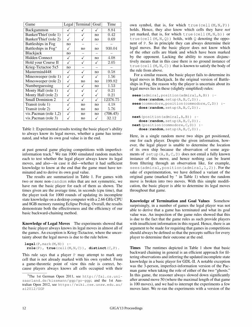
Table 1: Experimental results testing the basic player’s abilityto always know its legal moves, whether a game has termi-nated, and what its own goal value is in the end.
at past general game playing competitions with imperfect-information track.5 We ran 1000 simulated random matcheseach to test whether the legal player always knew its legalmoves, and also—in case it did—whether it had sufficientknowledge to know at the end that the game must have ter-minated and to derive its own goal value.
The results are summarized in Table 1. For games withtwo or more non-random roles that are not symmetric, wehave run the basic player for each of them as shown. Thetimes given are the average time, in seconds (cpu time), thatthe player took for 1000 rounds of updating its incompletestate knowledge on a desktop computer with a 2.66 GHz CPUand 8GB memory running Eclipse Prolog. Overall, the resultsdemonstrate both the effectiveness and the efficiency of ourbasic backward-chaining method.
Knowledge of Legal Moves The experiments showed thatthe basic player always knows its legal moves in almost all ofthe games. An exception is Krieg-Tictactoe, where the uncer-tainty about the legal moves is due to the rule below.
legal(P,mark(M,N)) :-role(P), true(cell(M,N,C)), distinct(C,P).
This rule says that a player P may attempt to mark anycell that is not already marked with his own symbol. Froma game-theoretic point of view this rule is correct, be-cause players always knows all cells occupied with their
5The 1st German Open 2011, see http://fai.cs.uni-saarland.de/kissmann/ggp/go-ggp; and the 1st Aus-tralian Open 2012, see https://wiki.cse.unsw.edu.au/ai2012/GGP
own symbol, that is, for which true(cell(M,N,P))holds. Hence, they also know which cells they have notyet marked, that is, for which true(cell(M,N,b)) ortrue(cell(M,N,Q)) holds, with Q denoting the oppo-nent of P. So in principle they can always determine theirlegal moves. But the basic player does not know whichof the other cells are blank and which have been markedby the opponent. Lacking the ability to reason disjunc-tively means that in this case there is no ground instance oftrue(cell(M,N,C)) that is known to satisfy the body ofthe rule from above.
For a similar reason, the basic player fails to determine itslegal moves in Blackjack. In the original version of Battle-ships in Fog, the reason why the player is uncertain about itslegal moves lies in these (slightly simplified) rules:
sees(admiral,position(admiral,A,B)) :-does(random,setup(A,B,C,D)).
sees(commodore,position(commodore,C,D)) :-does(random,setup(A,B,C,D)).
next(position(admiral,A,B)) :-does(random,setup(A,B,C,D)).
next(position(commodore,C,D)) :-does(random,setup(A,B,C,D)).
Here, in a single random move two ships get positioned,one for each player. Despite the given information, how-ever, the legal player is unable to determine the locationof its own ship because the observation of some argu-ments of setup(A,B,C,D) does not entail a fully knowninstance of this move, and hence nothing can be learntfrom filtering through an observation like, for example,sees(admiral,position(admiral,1,2)). For thesake of experimentation, we have defined a variant of theoriginal game (marked by ∗ in Table 1) where the randommove is broken into two moves. With this simple modifi-cation, the basic player is able to determine its legal movesthroughout that game.
Knowledge of Termination and Goal Values Somehowsurprisingly, in a number of games the legal player was notable to derive that a game has terminated and what its goalvalue was. An inspection of the game rules showed that thisis due to the fact that the game rules as such provide playerswith insufficient information in this regard. Hence, there is anargument to be made for requiring that games in competitionsshould always be defined so that the percepts suffice for everyplayer to determine their outcome at the end.
Times The runtimes depicted in Table 1 show that basicbackward chaining in general is an efficient approach for fil-tering observations and inferring the updated incomplete stateknowledge in a basic player for GDL-II. A notable exceptionwas the 3-person, imperfect-information version of the Pac-man game when taking the role of either of the two “ghosts.”In this game, the reasoner always slowed down significantlyafter around move 50 (where the maximal length of that gameis 100 moves), and we had to interrupt the experiments a fewmoves later. We re-ran the experiments with a version of the
GIGA'13 Proceedings12
basic player that only filters through the observations actu-ally made instead of also filtering through all non-percepts.The results given in Table 1 for “vis Pacman (role 1,2)” wereobtained for this simplified legal player.
ConclusionWe have developed a method for filtering with logic pro-grams and applied it to build a basic legal player for GDL-IIbased on backward-chaining. Our notion of filtering is simi-lar to [Amir and Russell, 2003; Shirazi and Amir, 2011]; intheir case a dynamic system is not described by logic pro-gram rules but in the Situation Calculus. For our backward-chaining filtering method we have adapted results for openlogic program from [Bonatti, 2001a; 2001b]. Our experi-ments showed that the method is sufficiently efficient in al-most all games from previous GGP competitions. It is worthstressing that even in games where the reasoner is not fastenough to be used at every node of a search tree, it can andin fact should be applied at least at the beginning in order toguarantee that the player submits a legal move. Our methodalso proved effective in almost all games, which supports anargument that can be made for it to be generally desirable thatall GDL-II games for competitions are written so that back-ward chaining augmented by support computation suffices toalways determine a player’s legal moves, as in our reformula-tion of Battleships in Fog.
Acknowledgements. This research was supported underAustralian Research Council’s Discovery Projects fundingscheme (project DP 120102023). The author is the recipientof an ARC Future Fellowship (project FT 0991348). He isalso affiliated with the University of Western Sydney.
References[Amir and Russell, 2003] Eyal Amir and Stuart Russell.
Logical filtering. In Proceedings of the International JointConference on Artificial Intelligence (IJCAI), pages 75–82, Acapulco, Mexico, August 2003. Morgan Kaufmann.
[Apt et al., 1987] Krzysztof Apt, H. Blair, and A. Walker.Towards a theory of declarative knowledge. In J. Minker,editor, Foundations of Deductive Databases and LogicProgramming, chapter 2, pages 89–148. Morgan Kauf-mann, 1987.
[Bonatti, 2001a] Piero Bonatti. Reasoning with open logicprograms. In T. Eiter, W. Faber, and M. Trusczynski, edi-tors, Proceedings of the International Conference on LogicProgramming and Nonmonotonic Reasoning (LPNMR),volume 2173 of LNCS, pages 147–159, Vienna, Austria,September 2001. Springer.
[Bonatti, 2001b] Piero Bonatti. Resolution with skepticalstable model semantics. Journal of Automated Reasoning,156(1):391–421, 2001.
[Edelkamp et al., 2012] Stefan Edelkamp, Tim Feder-holzner, and Peter Kissmann. Searching with partial beliefstates in general games with incomplete information. InB. Glimm and A. Kruger, editors, Proceedings of the
German Annual Conference on Artificial Intelligence(KI), volume 7526 of LNCS, pages 25–36, Saarbrucken,Germany, September 2012. Springer.
[Gelfond and Lifschitz, 1988] Michael Gelfond andVladimir Lifschitz. The stable model semantics forlogic programming. In R. Kowalski and K. Bowen,editors, Proceedings of the International Joint Conferenceand Symposium on Logic Programming (IJCSLP), pages1070–1080, Seattle, OR, 1988. MIT Press.
[Genesereth et al., 2005] Michael Genesereth, NathanielLove, and Barney Pell. General game playing: Overviewof the AAAI competition. AI Magazine, 26(2):62–72,2005.
[Kissmann and Edelkamp, 2010] Peter Kissmann and Ste-fan Edelkamp. Instantiating general games using Pro-log or dependency graphs. In R. Dillmann, J. Beyerer,U. Hanebeck, and T. Schultz, editors, Proceedings of theGerman Annual Conference on Artificial Intelligence (KI),volume 6359 of LNCS, pages 255–262, Karlsruhe, Ger-many, September 2010. Springer.
[Kleene, 1952] Stephen Kleene. Introduction to Metamathe-matics. Van Nostrand, New York, 1952.
[Lloyd and Topor, 1986] John Lloyd and R. Topor. A basisfor deductive database systems II. Journal of Logic Pro-gramming, 3(1):55–67, 1986.
[Lloyd, 1987] John Lloyd. Foundations of Logic Program-ming. Series Symbolic Computation. Springer, second,extended edition, 1987.
[Love et al., 2006] Nathaniel Love, Timothy Hinrichs, DavidHaley, Eric Schkufza, and Michael Genesereth. Gen-eral Game Playing: Game Description Language Speci-fication. Technical Report LG–2006–01, Stanford LogicGroup, Computer Science Department, Stanford Univer-sity, 353 Serra Mall, Stanford, CA 94305, 2006. Availableat: games.stanford.edu.
[Parker et al., 2005] Austin Parker, Dana Nau, and V.S. Sub-rahmanian. Game-tree search with combinatorially largebelief states. In L. Kaelbling and A. Saffiotti, editors, Pro-ceedings of the International Joint Conference on Artifi-cial Intelligence (IJCAI), pages 254–259, Edinburgh, UK,August 2005.
[Quenault and Cazenave, 2007] Michel Quenault and Tris-tan Cazenave. Extended general gaming model. In Com-puters Games Workshop, pages 195–2004, Amsterdam,June 2007.
[Richards and Amir, 2009] Mark Richards and Eyal Amir.Information set sampling in general imperfect informationpositional games. In Proceedings of the IJCAI Workshopon General Intelligence in Game-Playing Agents (GIGA),pages 59–66, Pasadena, 2009.
[Rosenhouse, 2009] Jason Rosenhouse. The Monty HallProblem. Oxford University Press, 2009.
[Saffidine and Cazenave, 2011] Abdallah Saffidine and Tris-tan Cazenave. A forward chaining based game descriptionlanguage compiler. In Proceedings of the IJCAI Workshop
GIGA'13 Proceedings 13
on General Intelligence in Game-Playing Agents (GIGA),pages 69–75, Barcelona, 2011.
[Schkufza et al., 2008] Eric Schkufza, Nathaniel Love, andMichael Genesereth. Propositional automata and cell au-tomata: Representational frameworks for discrete dynamicsystems. In Proceedings of the Australasian Joint Con-ference on Artificial Intelligence, volume 5360 of LNCS,pages 56–66, Auckland, December 2008. Springer.
[Schofield et al., 2012] Michael Schofield, TimothyCerexhe, and Michael Thielscher. HyperPlay: A solutionto general game playing with imperfect information.In Proceedings of the AAAI Conference on ArtificialIntelligence, pages 1606–1612, Toronto, July 2012. AAAIPress.
[Shepherdson, 1984] John C. Shepherdson. Negation as fail-ure: A comparison of Clark’s completed data base and Re-iter’s closed world assumption. Journal of Logic Program-ming, 1:51–79, 1984.
[Shirazi and Amir, 2011] Afsaneh Shirazi and Eyal Amir.First-order logical filtering. Artificial Intelligence,175(1):193–219, 2011.
[Silver and Veness, 2010] David Silver and Joel Veness.Monte-Carlo planning in large POMDPs. In J. Lafferty, C.Williams, J. Shawe-Taylor, R. Zemel, and A. Culotta, ed-itors, Advances in Neural Information Processing (NIPS),pages 2164–2172, Vancouver, Canada, December 2010.
[Thielscher, 2010] Michael Thielscher. A general game de-scription language for incomplete information games. InM. Fox and D. Poole, editors, Proceedings of the AAAIConference on Artificial Intelligence, pages 994–999, At-lanta, July 2010.
[Thielscher, 2011] Michael Thielscher. The general gameplaying description language is universal. In Proceedingsof the International Joint Conference on Artificial Intelli-gence (IJCAI), pages 1107–1112, Barcelona, July 2011.
[Waugh, 2009] Kevin Waugh. Faster state manipulation ingeneral games using generated code. In Proceedings of theIJCAI Workshop on General Intelligence in Game-PlayingAgents (GIGA), pages 91–97, Pasadena, 2009.
GIGA'13 Proceedings14
Sufficiency-Based Selection Strategy for MCTS ∗
Stefan Freyr Gudmundsson and Yngvi BjornssonSchool of Computer ScienceReykjavik University, Icelandstefang10,[email protected]
AbstractMonte-Carlo Tree Search (MCTS) has proved a re-markably effective decision mechanism in manydifferent game domains, including computer Goand general game playing (GGP). However, inGGP, where many disparate games are played, cer-tain type of games have proved to be particularlyproblematic for MCTS. One of the problems aregame trees with so-called optimistic moves, that is,bad moves that superficially look good but poten-tially require much simulation effort to prove oth-erwise. Such scenarios can be difficult to identify inreal time and can lead to suboptimal or even harm-ful decisions. In this paper we investigate a selec-tion strategy for MCTS to alleviate this problem.The strategy, called sufficiency threshold, concen-trates simulation effort better for resolving potentialoptimistic move scenarios. The improved strategyis evaluated empirically in an n-arm-bandit test do-main for highlighting its properties as well as in astate-of-the-art GGP agent to demonstrate its effec-tiveness in practice. The new strategy shows signif-icant improvements in both domains.
1 IntroductionFrom the inception of the field of Artificial Intelligence (AI),over half a century ago, games have played an importantrole as a testbed for advancements in the field, resulting ingame-playing systems that have reached or surpassed hu-mans in many games. A notable milestone was reachedwhen IBM’s chess program Deep Blue [Campbell et al.,2002] won a match against the number one chess player inthe world, Garry Kasparov, in 1997. The ’brain’ of DeepBlue relied heavily on both an efficient minimax-based game-tree search algorithm for thinking ahead and sophisticatedknowledge-based evaluation of game positions, using humanchess knowledge accumulated over centuries of play. A simi-lar approach has been used to build world-class programs formany other deterministic games, including Checkers [Scha-effer, 2009] and Othello [Buro, 1999].
∗This paper was also submitted (and accepted) to the main tech-nical track of IJCAI’13.
For non-deterministic games, in which moves may be sub-ject to chance, Monte-Carlo sampling methods have addition-ally been used to further improve decision quality. To accu-rately evaluate a position and the move options available, oneplays out (or samples) a large number of games as a part of theevaluation process. Backgammon is one example of a non-deterministic game, where possible moves are determined byrolls of dice, for which such an approach led to world-classcomputer programs (e.g., TD-Gammon [Tesauro, 1994]).
In recent years, a new simulation-based paradigm forgame-tree search has emerged, Monte-Carlo Tree Search(MCTS) [Coulom, 2006; Kocsis and Szepesvari, 2006].MCTS combines elements from both traditional game-tree search and Monte-Carlo simulations to form a full-fledged best-first search procedure. Many games, both non-deterministic and deterministic, lend themselves well to theMCTS approach. As an example, MCTS has in the pastfew years greatly enhanced the state of the art of computerGo [Enzenberger and Muller, 2009], a game that has eludedcomputer based approaches so far.
MCTS has also been used successfully in General GamePlaying (GGP) [Genesereth et al., 2005]. The goal thereis to create intelligent agents that can automatically learnhow to skillfully play a wide variety of games, givenonly the descriptions of the game rules (in a languagecalled GDL [Love et al., 2008]). This requires that theagents learn diverse game-playing strategies without anygame-specific knowledge being provided by their develop-ers. Most of the strongest GGP agents are now MCTS-based, such as ARY [Mehat and Cazenave, 2011], CA-DIAPLAYER [Bjornsson and Finnsson, 2009; Finnsson andBjornsson, 2011a], MALIGNE [Kirci et al., 2011], and TUR-BOTURTLE. Although MCTS have proved on average moreeffective than traditional heuristic-based game-tree search inGGP, there is still a large number of game domains where itdoes not work nearly as well, for example in non-progressingor highly tactical (chess-like) games. The more general con-cept of optimistic actions, encapsulating among other thingstactical traps, is by and large problematic for MCTS [Ra-manujan et al., 2010; Finnsson and Bjornsson, 2011b].
In this paper we propose an improved selection strategyfor MCTS, sufficiency-threshold, that is more effective in do-mains troubled with optimistic actions and, generally speak-ing, more robust on the whole. We also take steps towards
GIGA'13 Proceedings 15
better understanding how determinism and discrete game out-comes affect the action-selection mechanism of MCTS, andthen empirically evaluate the sufficiency-threshold strategy insuch domains, where it shows significant improvements.
The paper is structured as follows. In the next section weprovide necessary background material, then we discuss suf-ficiently good moves and the sufficiency-threshold strategy.This is followed by an empirical evaluation of the strategy inboth an n-arm-bandit setup and GGP. Finally, we concludeand discuss future work.
2 BackgroundBefore we introduce our new selection strategy we first pro-vide the necessary background on MCTS, optimistic actions,and n-arm-bandits (which we use as a part of the experimen-tal evaluation of the new selection strategy).
2.1 Monte-Carlo Tree SearchMonte-Carlo Tree Search (MCTS) is a simulation-basedsearch technique that extends Monte-Carlo simulations to bebetter suited for (adversary) games. It starts by running apure Monte-Carlo simulation, but gradually builds a gametree in memory with each new simulation. This allows for amore informed mechanism where each simulation consists offour strategic steps: selection, expansion, playout, and back-propagation. In the selection step, the tree is traversed fromthe root of the game tree until a leave node is reached, wherethe expansion step expands the leave by one level (typicallyadding only a single node). From the newly added node aregular Monte-Carlo playout is run until the end of the game(or when some other terminating condition is met), at whichpoint the result is back-propagated back up to the root mod-ifying the statistics stored in the game tree as appropriate.MCTS continues to run such four step simulations until de-liberation time is up, at which point the most promising actionof the root node is played.
In this paper we are mainly concerned with the selec-tion step, where Upper Confidence-bounds applied to Trees(UCT) [Kocsis and Szepesvari, 2006] is widely used for ac-tion selection. At each internal node in the game tree an ac-tion a∗ to simulate is chosen as follows:
a∗ = argmaxa∈A(s)
Q(s, a) + C
√lnN(s)
N(s, a)
(1)
N(s) stands for the number of samples gathered in state sand N(s, a) for number of samples gathered when takingaction a in state s. A(s) is the set of possible actions instate s and Q(s, a) is the expected return for action a in states, usually the arithmetic mean of the N(s, a) samples gath-ered for action a. The term added to Q(s, a) decides howmuch we are willing to explore, where the constantC dictateshow much effect the exploration term has versus exploitation.With C = 0 our samples would be gathered greedily, alwaysselecting the top-rated action for each playout. When we havevalues of N(s, a) which are not defined, we consider the ex-ploration term as being infinity.
Although MCTS is effective in many game domains, ithas difficulties in other common game structures. Several
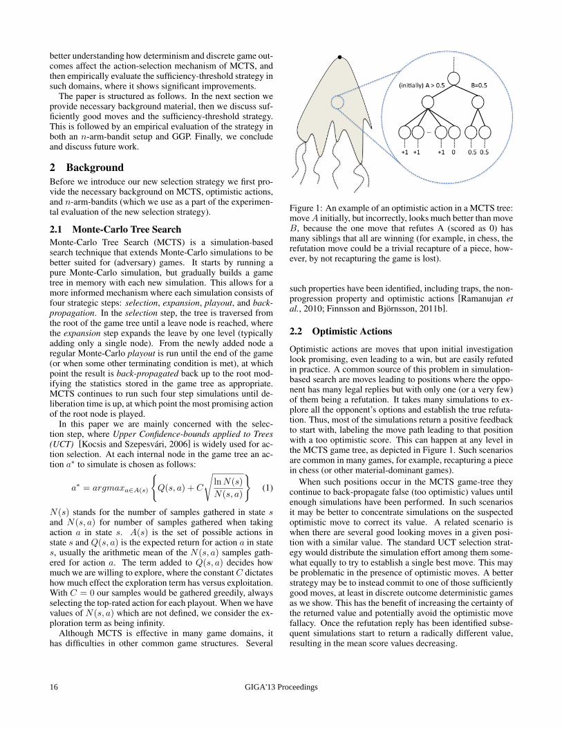
Figure 1: An example of an optimistic action in a MCTS tree:moveA initially, but incorrectly, looks much better than moveB, because the one move that refutes A (scored as 0) hasmany siblings that all are winning (for example, in chess, therefutation move could be a trivial recapture of a piece, how-ever, by not recapturing the game is lost).
such properties have been identified, including traps, the non-progression property and optimistic actions [Ramanujan etal., 2010; Finnsson and Bjornsson, 2011b].
2.2 Optimistic Actions
Optimistic actions are moves that upon initial investigationlook promising, even leading to a win, but are easily refutedin practice. A common source of this problem in simulation-based search are moves leading to positions where the oppo-nent has many legal replies but with only one (or a very few)of them being a refutation. It takes many simulations to ex-plore all the opponent’s options and establish the true refuta-tion. Thus, most of the simulations return a positive feedbackto start with, labeling the move path leading to that positionwith a too optimistic score. This can happen at any level inthe MCTS game tree, as depicted in Figure 1. Such scenariosare common in many games, for example, recapturing a piecein chess (or other material-dominant games).
When such positions occur in the MCTS game-tree theycontinue to back-propagate false (too optimistic) values untilenough simulations have been performed. In such scenariosit may be better to concentrate simulations on the suspectedoptimistic move to correct its value. A related scenario iswhen there are several good looking moves in a given posi-tion with a similar value. The standard UCT selection strat-egy would distribute the simulation effort among them some-what equally to try to establish a single best move. This maybe problematic in the presence of optimistic moves. A betterstrategy may be to instead commit to one of those sufficientlygood moves, at least in discrete outcome deterministic gamesas we show. This has the benefit of increasing the certainty ofthe returned value and potentially avoid the optimistic movefallacy. Once the refutation reply has been identified subse-quent simulations start to return a radically different value,resulting in the mean score values decreasing.
GIGA'13 Proceedings16
2.3 N -arm-bandit and the Mean’s PathTo simulate a decision process for choosing moves in a gamewe can think of a one-arm-bandit problem. We stand in frontof a number of one-arm-bandits, slot machines, with coins toplay with. Each bandit has its own probability distributionwhich is unknown to us. The question is, how do we max-imize our profit? We start by playing the bandits to gathersome information. Then, we have to decide where to put ourlimited amount of coins. This becomes a matter of balanc-ing between exploiting and exploring, i.e. play greedily andtry less promising bandits. The selection formula (Equation1) is derived from this setup [Kocsis and Szepesvari, 2006].Instead of n one-arm-bandits we can equally talk about onen-arm-bandit and we will use that terminology henceforth.
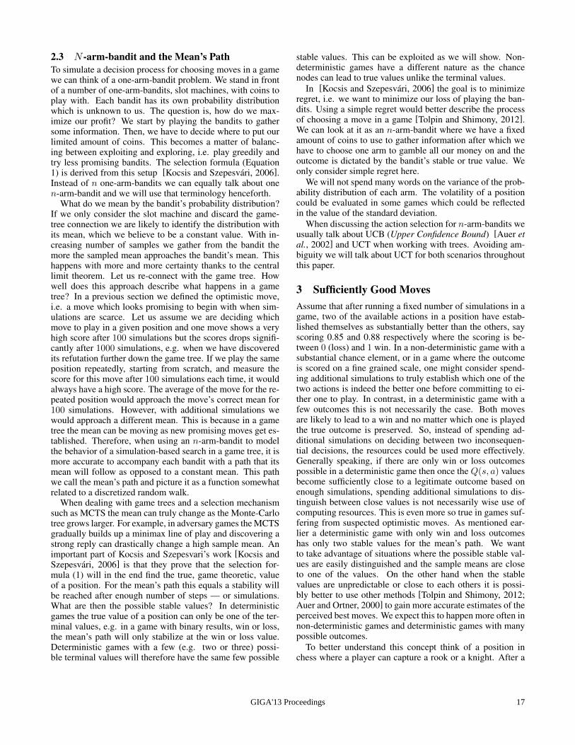
What do we mean by the bandit’s probability distribution?If we only consider the slot machine and discard the game-tree connection we are likely to identify the distribution withits mean, which we believe to be a constant value. With in-creasing number of samples we gather from the bandit themore the sampled mean approaches the bandit’s mean. Thishappens with more and more certainty thanks to the centrallimit theorem. Let us re-connect with the game tree. Howwell does this approach describe what happens in a gametree? In a previous section we defined the optimistic move,i.e. a move which looks promising to begin with when sim-ulations are scarce. Let us assume we are deciding whichmove to play in a given position and one move shows a veryhigh score after 100 simulations but the scores drops signifi-cantly after 1000 simulations, e.g. when we have discoveredits refutation further down the game tree. If we play the sameposition repeatedly, starting from scratch, and measure thescore for this move after 100 simulations each time, it wouldalways have a high score. The average of the move for the re-peated position would approach the move’s correct mean for100 simulations. However, with additional simulations wewould approach a different mean. This is because in a gametree the mean can be moving as new promising moves get es-tablished. Therefore, when using an n-arm-bandit to modelthe behavior of a simulation-based search in a game tree, it ismore accurate to accompany each bandit with a path that itsmean will follow as opposed to a constant mean. This pathwe call the mean’s path and picture it as a function somewhatrelated to a discretized random walk.
When dealing with game trees and a selection mechanismsuch as MCTS the mean can truly change as the Monte-Carlotree grows larger. For example, in adversary games the MCTSgradually builds up a minimax line of play and discovering astrong reply can drastically change a high sample mean. Animportant part of Kocsis and Szepesvari’s work [Kocsis andSzepesvari, 2006] is that they prove that the selection for-mula (1) will in the end find the true, game theoretic, valueof a position. For the mean’s path this equals a stability willbe reached after enough number of steps — or simulations.What are then the possible stable values? In deterministicgames the true value of a position can only be one of the ter-minal values, e.g. in a game with binary results, win or loss,the mean’s path will only stabilize at the win or loss value.Deterministic games with a few (e.g. two or three) possi-ble terminal values will therefore have the same few possible
stable values. This can be exploited as we will show. Non-deterministic games have a different nature as the chancenodes can lead to true values unlike the terminal values.
In [Kocsis and Szepesvari, 2006] the goal is to minimizeregret, i.e. we want to minimize our loss of playing the ban-dits. Using a simple regret would better describe the processof choosing a move in a game [Tolpin and Shimony, 2012].We can look at it as an n-arm-bandit where we have a fixedamount of coins to use to gather information after which wehave to choose one arm to gamble all our money on and theoutcome is dictated by the bandit’s stable or true value. Weonly consider simple regret here.
We will not spend many words on the variance of the prob-ability distribution of each arm. The volatility of a positioncould be evaluated in some games which could be reflectedin the value of the standard deviation.
When discussing the action selection for n-arm-bandits weusually talk about UCB (Upper Confidence Bound) [Auer etal., 2002] and UCT when working with trees. Avoiding am-biguity we will talk about UCT for both scenarios throughoutthis paper.
3 Sufficiently Good MovesAssume that after running a fixed number of simulations in agame, two of the available actions in a position have estab-lished themselves as substantially better than the others, sayscoring 0.85 and 0.88 respectively where the scoring is be-tween 0 (loss) and 1 win. In a non-deterministic game with asubstantial chance element, or in a game where the outcomeis scored on a fine grained scale, one might consider spend-ing additional simulations to truly establish which one of thetwo actions is indeed the better one before committing to ei-ther one to play. In contrast, in a deterministic game with afew outcomes this is not necessarily the case. Both movesare likely to lead to a win and no matter which one is playedthe true outcome is preserved. So, instead of spending ad-ditional simulations on deciding between two inconsequen-tial decisions, the resources could be used more effectively.Generally speaking, if there are only win or loss outcomespossible in a deterministic game then once the Q(s, a) valuesbecome sufficiently close to a legitimate outcome based onenough simulations, spending additional simulations to dis-tinguish between close values is not necessarily wise use ofcomputing resources. This is even more so true in games suf-fering from suspected optimistic moves. As mentioned ear-lier a deterministic game with only win and loss outcomeshas only two stable values for the mean’s path. We wantto take advantage of situations where the possible stable val-ues are easily distinguished and the sample means are closeto one of the values. On the other hand when the stablevalues are unpredictable or close to each others it is possi-bly better to use other methods [Tolpin and Shimony, 2012;Auer and Ortner, 2000] to gain more accurate estimates of theperceived best moves. We expect this to happen more often innon-deterministic games and deterministic games with manypossible outcomes.
To better understand this concept think of a position inchess where a player can capture a rook or a knight. After a
GIGA'13 Proceedings 17
0 100 200 300 400 500
0
0.5
1
Samples(k)
Me
an
va
lue
True value 0
True value 1
(a) Two types of mean’s pathfollowing a random walk
0 500 1000 1500 2000 2500 3000
0
25
50
75
100
Samples (k)
% o
f o
ptim
al p
lay
20 arms − 10% winners
20 arms − 30% winners
50 arms − 10% winners
50 arms − 30% winners
(b) UCT with various numberof arms and winners
Figure 2: Two examples of mean’s paths and ratio of optimalplay using UCT
few simulations we get high estimates for both moves. Prob-abilities are that both lead to a win, i.e. both might have thesame true value as 1. For humans it is possibly easier to se-cure the victory by capturing the rook but we are more inter-ested in knowing whether there is a dangerous reply lurkingjust beyond our horizon, i.e. whether one of the moves is anoptimistic move. We argue that at this point it is more impor-tant to get more reliable information about one of the movesinstead of trying to distinguish between, possibly, close toequally good moves. Either our estimate of one of the movesstays high or even gets higher and our confidence increases orthe estimate drops and we have proven the original estimatewrong which can be equally important. We introduce a suf-ficiency threshold α such that whenever we have an estimateQ(s, a) > α from (1) we say that this move is sufficientlygood and therefore unplug the exploration. To do so we re-place C in Equation (1) by C as follows:
C =
C when all Q(s, a) ≤ α,0 when any Q(s, a) > α.
(2)
We call this method sufficiency threshold (ST). When our es-timates drop below the sufficiency threshold we go back tothe original UCT method. For unclear or bad positions whereestimates are less than α most of the time, showing occa-sional spikes, this approach differs from UCT in temporarilyrearranging the order of moves to sample. After such a rear-rangement the methods more or less couple back to selectingthe same moves to sample from.
4 ExperimentsWe empirically evaluated the ST selection strategy in threedifferent scenarios: an n-arm-bandit to clearly demonstrateits properties, a sample game position demonstrating its po-tentials in alleviating problems caused by optimistic moves,and finally in a simulation-based GGP agent to show its ef-fectiveness on a variety of games.
4.1 N -arm-bandit ExperimentsIn our n-arm-bandits experiment we consider only true values0 and 1. With each sample we gather for a bandit we moveone step further along the mean’s path.
Our setup is related to Sutton and Barto’s approach (1998)but adapted for deterministic environments. Once a path
0 500 1000 1500 2000 2500 3000
−4
−2
0
2
4
6
8
Samples (k)
±%
ST − UCT
95% confidence
(a) ST vs UCT (10% win)
0 500 1000 1500 2000 2500 3000
−4
−2
0
2
4
6
8
Samples (k)
±%
ST − UCT
95% confidence
(b) ST vs UCT (30% win)
Figure 3: 20 arms
0 500 1000 1500 2000 2500 3000
−4
−2
0
2
4
6
8
Samples (k)
±%
ST − UCT
95% confidence
(a) ST vs UCT (10% win)
0 500 1000 1500 2000 2500 3000
−4
−2
0
2
4
6
8
Samples (k)
±%
ST − UCT
95% confidence
(b) ST vs UCT (30% win)
Figure 4: 50 arms
reaches 0 or 1 it has found its true value and does not changeafter that. This way we get closer to the true value of a banditthe more samples we gather from it. Figure 2a shows pos-sible paths hitting 0 or 1. We let Mi(ki) be the mean valuefor bandit i after ki samples. The total number of samples isk =
∑i ki. We use the results from the samples to evaluate
the expected rewards of the bandits. Let Qi(k) play the samerole as Q(s, a) in (1), i.e. be the expected reward for bandit iafter k samples. For each k we record which arm we wouldchoose for our final bet, i.e. with the highest Qi(k) value.
We experiment with a bandit as follows. Pulling an armonce is a sample. A single task is to gather information for ksamples, k ∈ [1, 3000]. For each sample we measure whichaction an agent would take at that point, i.e. which banditwould we gamble all our money on with current informationavailable to us. Let V (k) be the value of the action takenafter gathering k samples. V (k) = 1 if the chosen bandit hasa true value of 1 and V (k) = 0 otherwise. A trial consists ofrunning t tasks and calculate the mean value of V (k) for eachk ∈ [1, 3000]. This gives us one measurement, V (k), whichmeasures the ratio of optimal play for an agent with respectto k. There is always at least one bandit with a true value of1. Each trial is for a single n-arm-bandit, representing onetype of a position in a game. In the experiments that followwe compare the performance of ST to UCT, using parametersettings of C = 0.4 and α = 0.6.
We run experiments on 50 different bandits (models) gen-erated randomly as follows. All the arms start with Mi(1) =0.5 and have randomly generated mean’s paths although con-strained such that they hit loss (0) or win (1) before taking 500steps. The step size is 0.02 and each step is equally likely tobe positive or negative. One trial consisting of 200 tasks is
GIGA'13 Proceedings18
run for each bandit, giving us 50 measurements of V (k) foreach agent and each k ∈ [1, 3000]. In the following charts weshow a 95% confidence interval over the models.
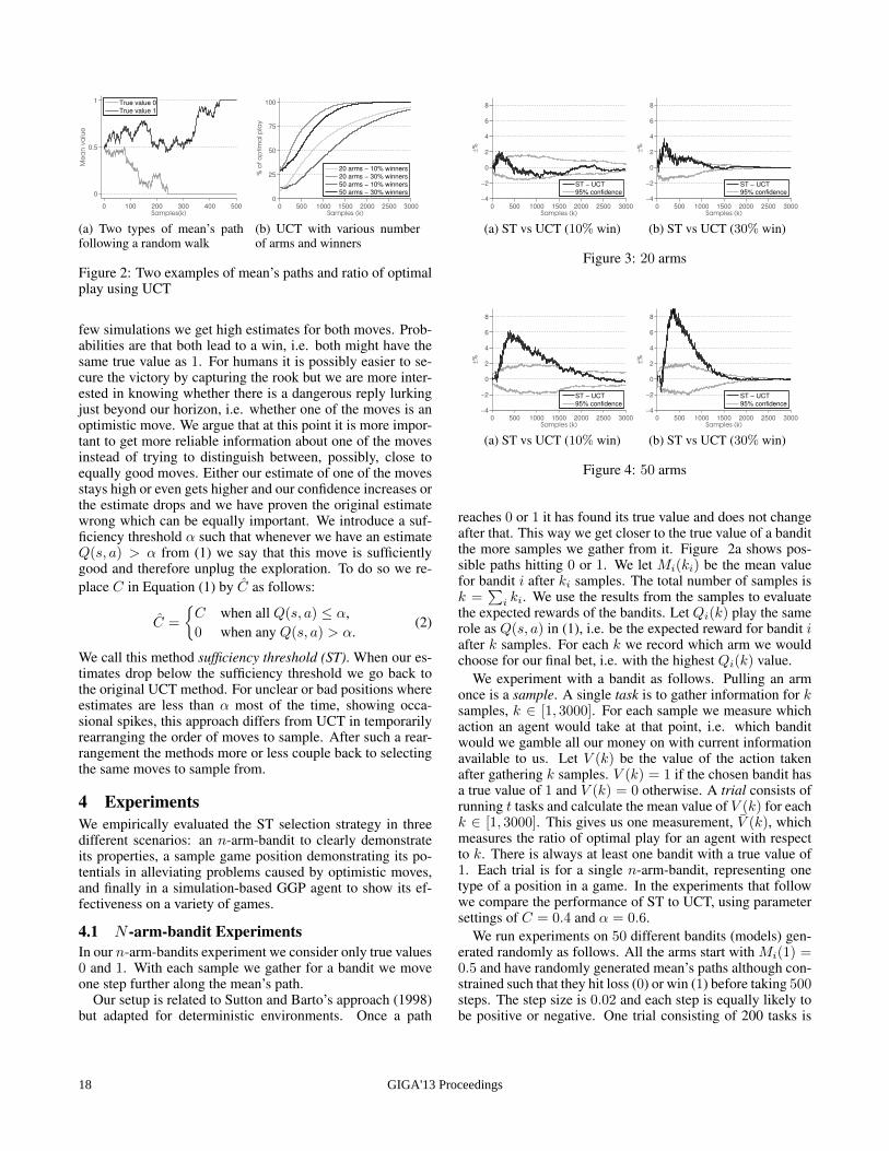
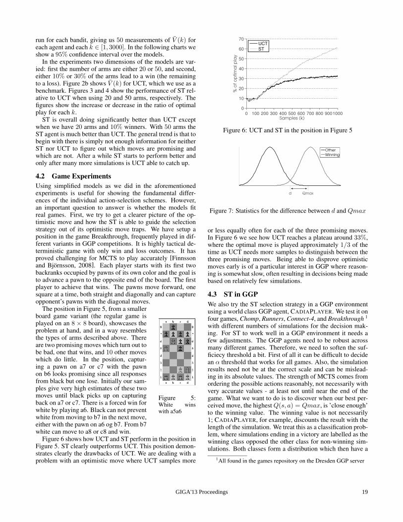
In the experiments two dimensions of the models are var-ied: first the number of arms are either 20 or 50, and second,either 10% or 30% of the arms lead to a win (the remainingto a loss). Figure 2b shows V (k) for UCT, which we use as abenchmark. Figures 3 and 4 show the performance of ST rel-ative to UCT when using 20 and 50 arms, respectively. Thefigures show the increase or decrease in the ratio of optimalplay for each k.
ST is overall doing significantly better than UCT exceptwhen we have 20 arms and 10% winners. With 50 arms theST agent is much better than UCT. The general trend is that tobegin with there is simply not enough information for neitherST nor UCT to figure out which moves are promising andwhich are not. After a while ST starts to perform better andonly after many more simulations is UCT able to catch up.
4.2 Game ExperimentsUsing simplified models as we did in the aforementionedexperiments is useful for showing the fundamental differ-ences of the individual action-selection schemes. However,an important question to answer is whether the models fitreal games. First, we try to get a clearer picture of the op-timistic move and how the ST is able to guide the selectionstrategy out of its optimistic move traps. We have setup aposition in the game Breakthrough, frequently played in dif-ferent variants in GGP competitions. It is highly tactical de-terministic game with only win and loss outcomes. It hasproved challenging for MCTS to play accurately [Finnssonand Bjornsson, 2008]. Each player starts with its first twobackranks occupied by pawns of its own color and the goal isto advance a pawn to the opposite end of the board. The firstplayer to achieve that wins. The pawns move forward, onesquare at a time, both straight and diagonally and can captureopponent’s pawns with the diagonal moves.
Figure 5:White winswith a5a6
The position in Figure 5, from a smallerboard game variant (the regular game isplayed on an 8 × 8 board), showcases theproblem at hand, and in a way resemblesthe types of arms described above. Thereare two promising moves which turn out tobe bad, one that wins, and 10 other moveswhich do little. In the position, captur-ing a pawn on a7 or c7 with the pawnon b6 looks promising since all responsesfrom black but one lose. Initially our sam-ples give very high estimates of these twomoves until black picks up on capturingback on a7 or c7. There is a forced win forwhite by playing a6. Black can not preventwhite from moving to b7 in the next move,either with the pawn on a6 og b7. From b7white can move to a8 or c8 and win.
Figure 6 shows how UCT and ST perform in the position inFigure 5. ST clearly outperforms UCT. This position demon-strates clearly the drawbacks of UCT. We are dealing with aproblem with an optimistic move where UCT samples more
0 100 200 300 400 500 600 700 800 9001000
0
10
20
30
40
50
60
70
Samples (k)
% o
f o
ptim
al p
lay
UCT
ST
Figure 6: UCT and ST in the position in Figure 5
d Qmax
Other
Winning
Figure 7: Statistics for the difference between d and Qmax
or less equally often for each of the three promising moves.In Figure 6 we see how UCT reaches a plateau around 33%,where the optimal move is played approximately 1/3 of thetime as UCT needs more samples to distinguish between thethree promising moves. Being able to disprove optimisticmoves early is of a particular interest in GGP where reason-ing is somewhat slow, often resulting in decisions being madebased on relatively few simulations.
4.3 ST in GGPWe also try the ST selection strategy in a GGP environmentusing a world class GGP agent, CADIAPLAYER. We test it onfour games, Chomp, Runners, Connect-4, and Breakthrough 1
with different numbers of simulations for the decision mak-ing. For ST to work well in a GGP environment it needs afew adjustments. The GGP agents need to be robust acrossmany different games. Therefore, we need to soften the suf-ficiecy threshold a bit. First of all it can be difficult to decidean α threshold that works for all games. Also, the simulationresults need not be at the correct scale and can be mislead-ing in its absolute values. The strength of MCTS comes fromordering the possible actions reasonably, not necessarily withvery accurate values - at least not until near the end of thegame. What we want to do is to discover when our best per-ceived move, the highestQ(s, a) = Qmax, is ’close enough’to the winning value. The winning value is not necessarily1; CADIAPLAYER, for example, discounts the result with thelength of the simulation. We treat this as a classification prob-lem, where simulations ending in a victory are labelled as thewinning class opposed the other class for non-winning sim-ulations. Both classes form a distribution which then have a
1All found in the games repository on the Dresden GGP server
GIGA'13 Proceedings 19
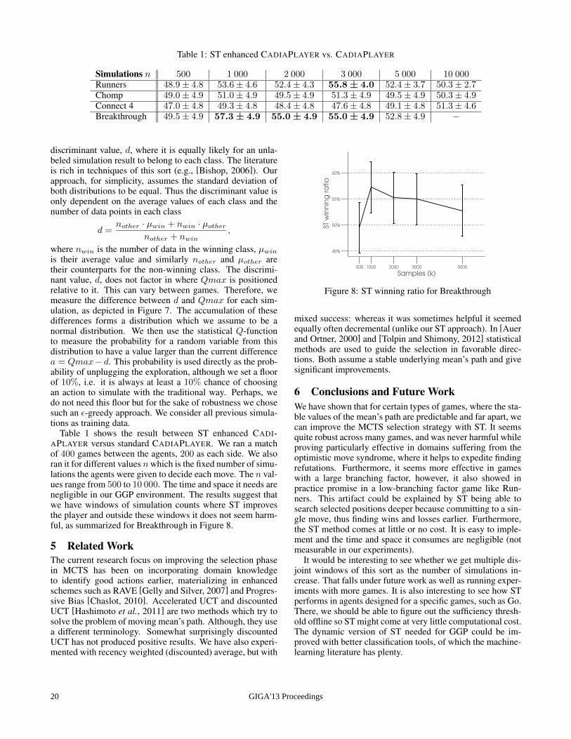
Table 1: ST enhanced CADIAPLAYER vs. CADIAPLAYER
Simulations n 500 1 000 2 000 3 000 5 000 10 000Runners 48.9± 4.8 53.6± 4.6 52.4± 4.3 55.8 ± 4.0 52.4± 3.7 50.3± 2.7Chomp 49.0± 4.9 51.0± 4.9 49.5± 4.9 51.3± 4.9 49.5± 4.9 50.3± 4.9Connect 4 47.0± 4.8 49.3± 4.8 48.4± 4.8 47.6± 4.8 49.1± 4.8 51.3± 4.6Breakthrough 49.5± 4.9 57.3 ± 4.9 55.0 ± 4.9 55.0 ± 4.9 52.8± 4.9 −
discriminant value, d, where it is equally likely for an unla-beled simulation result to belong to each class. The literatureis rich in techniques of this sort (e.g., [Bishop, 2006]). Ourapproach, for simplicity, assumes the standard deviation ofboth distributions to be equal. Thus the discriminant value isonly dependent on the average values of each class and thenumber of data points in each class
d =nother · µwin + nwin · µother
nother + nwin,
where nwin is the number of data in the winning class, µwin
is their average value and similarly nother and µother aretheir counterparts for the non-winning class. The discrimi-nant value, d, does not factor in where Qmax is positionedrelative to it. This can vary between games. Therefore, wemeasure the difference between d and Qmax for each sim-ulation, as depicted in Figure 7. The accumulation of thesedifferences forms a distribution which we assume to be anormal distribution. We then use the statistical Q-functionto measure the probability for a random variable from thisdistribution to have a value larger than the current differencea = Qmax− d. This probability is used directly as the prob-ability of unplugging the exploration, although we set a floorof 10%, i.e. it is always at least a 10% chance of choosingan action to simulate with the traditional way. Perhaps, wedo not need this floor but for the sake of robustness we chosesuch an ε-greedy approach. We consider all previous simula-tions as training data.
Table 1 shows the result between ST enhanced CADI-APLAYER versus standard CADIAPLAYER. We ran a matchof 400 games between the agents, 200 as each side. We alsoran it for different values nwhich is the fixed number of simu-lations the agents were given to decide each move. The n val-ues range from 500 to 10 000. The time and space it needs arenegligible in our GGP environment. The results suggest thatwe have windows of simulation counts where ST improvesthe player and outside these windows it does not seem harm-ful, as summarized for Breakthrough in Figure 8.
5 Related WorkThe current research focus on improving the selection phasein MCTS has been on incorporating domain knowledgeto identify good actions earlier, materializing in enhancedschemes such as RAVE [Gelly and Silver, 2007] and Progres-sive Bias [Chaslot, 2010]. Accelerated UCT and discountedUCT [Hashimoto et al., 2011] are two methods which try tosolve the problem of moving mean’s path. Although, they usea different terminology. Somewhat surprisingly discountedUCT has not produced positive results. We have also experi-mented with recency weighted (discounted) average, but with
500 1000 2000 3000 5000
45%
50%
55%
60%
ST
win
nin
g r
atio
Samples (k)
Figure 8: ST winning ratio for Breakthrough
mixed success: whereas it was sometimes helpful it seemedequally often decremental (unlike our ST approach). In [Auerand Ortner, 2000] and [Tolpin and Shimony, 2012] statisticalmethods are used to guide the selection in favorable direc-tions. Both assume a stable underlying mean’s path and givesignificant improvements.
6 Conclusions and Future WorkWe have shown that for certain types of games, where the sta-ble values of the mean’s path are predictable and far apart, wecan improve the MCTS selection strategy with ST. It seemsquite robust across many games, and was never harmful whileproving particularly effective in domains suffering from theoptimistic move syndrome, where it helps to expedite findingrefutations. Furthermore, it seems more effective in gameswith a large branching factor, however, it also showed inpractice promise in a low-branching factor game like Run-ners. This artifact could be explained by ST being able tosearch selected positions deeper because committing to a sin-gle move, thus finding wins and losses earlier. Furthermore,the ST method comes at little or no cost. It is easy to imple-ment and the time and space it consumes are negligible (notmeasurable in our experiments).
It would be interesting to see whether we get multiple dis-joint windows of this sort as the number of simulations in-crease. That falls under future work as well as running exper-iments with more games. It is also interesting to see how STperforms in agents designed for a specific games, such as Go.There, we should be able to figure out the sufficiency thresh-old offline so ST might come at very little computational cost.The dynamic version of ST needed for GGP could be im-proved with better classification tools, of which the machine-learning literature has plenty.
GIGA'13 Proceedings20
References[Auer and Ortner, 2000] Peter Auer and Ronald Ortner. Ucb
revisited: Improved regret bounds for the stochastic multi-armed bandit problem, 2000.
[Auer et al., 2002] Peter Auer, Nicolo Cesa-Bianchi, andPaul Fischer. Finite-time analysis of the multiarmed banditproblem. Machine Learning, 47(2/3):235–256, 2002.
[Bishop, 2006] C. M. Bishop. Pattern Recognition and Ma-chine Learning. Springer, 2006.
[Bjornsson and Finnsson, 2009] Yngvi Bjornsson andHilmar Finnsson. Cadiaplayer: A simulation-basedgeneral game player. IEEE Trans. Comput. Intellig. andAI in Games, 1(1):4–15, 2009.
[Buro, 1999] Michael Buro. How machines have learnedto play Othello. IEEE Intelligent Systems, 14(6):12–14,November/December 1999. Research Note.
[Campbell et al., 2002] Murray Campbell, A. Joseph Hoane,Jr., and Feng-Hsiung Hsu. Deep blue. Artificial Intelli-gence, 134(1–2):57–83, 2002.
[Chaslot, 2010] Guillaume Chaslot. Monte-Carlo TreeSearch. PhD dissertation, Maastricht University, TheNetherlands, Department of Knowledge Engineering,2010.
[Coulom, 2006] Remi Coulom. Efficient selectivity andbackup operators in monte-carlo tree search. In H. Jaapvan den Herik, Paolo Ciancarini, and H. H. L. M. Donkers,editors, Computers and Games, volume 4630 of LectureNotes in Computer Science, pages 72–83. Springer, 2006.
[Enzenberger and Muller, 2009] Markus Enzenberger andMartin Muller. Fuego - an open-source framework forboard games and go engine based on monte-carlo treesearch. Technical Report 09-08, Dept. of Computing Sci-ence, University of Alberta, 2009.
[Finnsson and Bjornsson, 2008] Hilmar Finnsson and YngviBjornsson. Simulation-based approach to general gameplaying. In Dieter Fox and Carla P. Gomes, editors, Pro-ceedings of the Twenty-Third AAAI Conference on Arti-ficial Intelligence, AAAI 2008, Chicago, Illinois, USA,July 13-17, 2008, pages 259–264, Cambridge, MA, USA,2008. AAAI Press.
[Finnsson and Bjornsson, 2011a] Hilmar Finnsson and Yn-gvi Bjornsson. Cadiaplayer: Search-control techniques.KI, 25(1):9–16, 2011.
[Finnsson and Bjornsson, 2011b] Hilmar Finnsson and Yn-gvi Bjornsson. Game-tree properties and mcts perfor-mance. In IJCAI’11 Workshop on General Intelligence inGame Playing Agents (GIGA’11), pages 23–30, 2011.
[Gelly and Silver, 2007] Sylvain Gelly and David Silver.Combining online and offline knowledge in uct. In Pro-ceedings of the 24th international conference on Machinelearning, ICML ’07, pages 273–280, New York, NY, USA,2007. ACM.
[Genesereth et al., 2005] Michael R. Genesereth, NathanielLove, and Barney Pell. General Game Playing: Overview
of the AAAI competition. AI Magazine, 26(2):62–72,2005.
[Hashimoto et al., 2011] Junichi Hashimoto, Akihiro Kishi-moto, Kazuki Yoshizoe, and Kokolo Ikeda. AcceleratedUCT and its application to two-player games. In H. Jaapvan den Herik and Aske Plaat, editors, ACG, volume7168 of Lecture Notes in Computer Science, pages 1–12.Springer, 2011.
[Kirci et al., 2011] Mesut Kirci, Nathan R. Sturtevant, andJonathan Schaeffer. A GGP feature learning algorithm.KI, 25(1):35–42, 2011.
[Kocsis and Szepesvari, 2006] Levante Kocsis and CsabaSzepesvari. Bandit based Monte-Carlo planning. In Eu-ropean Conference on Machine Learning (ECML), pages282–293, Berlin / Heidelberg, 2006. Springer.
[Love et al., 2008] Nathaniel Love, Timothy Hinrichs,David Haley, Eric Schkufza, and Michael Genesereth.General game playing: Game description languagespecification. Technical report, Stanford University,2008. most recent version should be available athttp://games.stanford.edu/.
[Mehat and Cazenave, 2011] Jean Mehat and TristanCazenave. A parallel general game player. KI, 25(1):43–47, 2011.
[Ramanujan et al., 2010] Raghuram Ramanujan, AshishSabharwal, and Bart Selman. On adversarial search spacesand sampling-based planning. In ICAPS, pages 242–245,2010.
[Schaeffer, 2009] Jonathan Schaeffer. One JumpAhead:Computer Perfection at Checkers. Springer,2009.
[Sutton and Barto, 1998] Richard Sutton and A. Barto. Re-inforcement Learning: An Introduction. MIT press, Cam-bridge, MA, USA, 1998.
[Tesauro, 1994] Gerald Tesauro. TD-Gammon, a self-teaching backgammon program, achieves master-levelplay. Neural Comput., 6(2):215–219, 1994.
[Tolpin and Shimony, 2012] David Tolpin and Solomon EyalShimony. Mcts based on simple regret. CoRR,abs/1207.5536, 2012.
GIGA'13 Proceedings 21

GIGA'13 Proceedings22
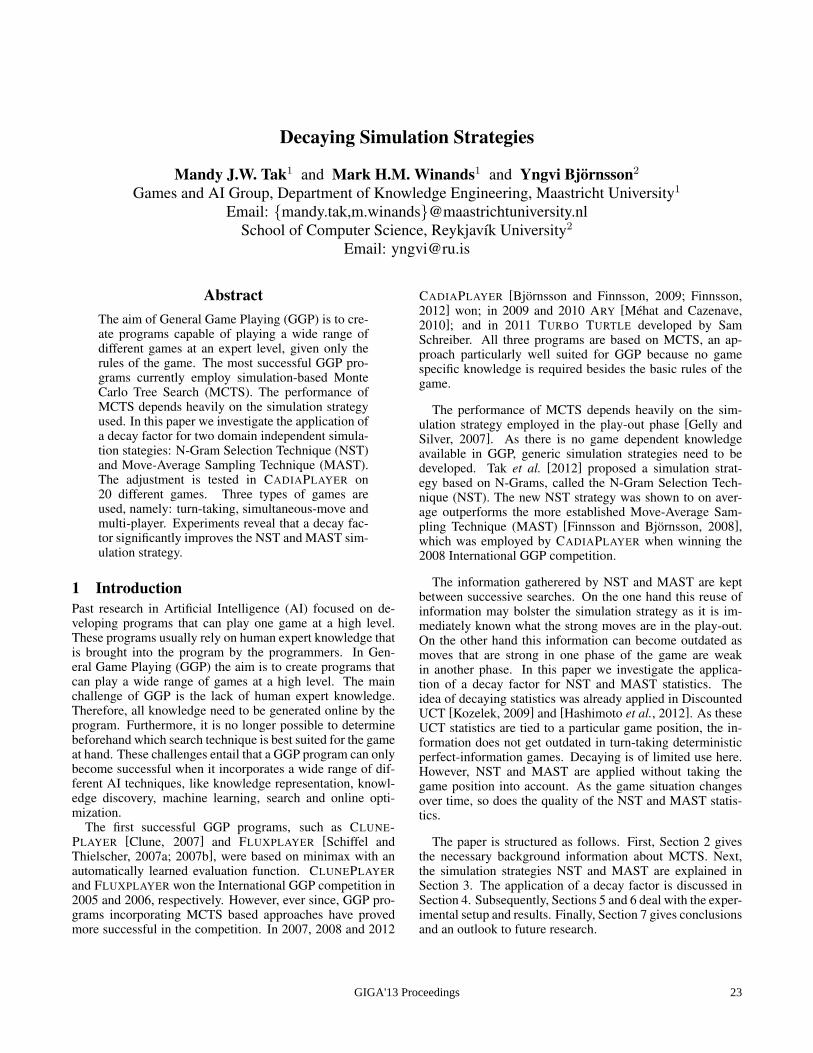
Decaying Simulation Strategies
Mandy J.W. Tak1 and Mark H.M. Winands1 and Yngvi Bjornsson2
Games and AI Group, Department of Knowledge Engineering, Maastricht University1
Email: mandy.tak,[email protected] of Computer Science, Reykjavık University2
Email: [email protected]
AbstractThe aim of General Game Playing (GGP) is to cre-ate programs capable of playing a wide range ofdifferent games at an expert level, given only therules of the game. The most successful GGP pro-grams currently employ simulation-based MonteCarlo Tree Search (MCTS). The performance ofMCTS depends heavily on the simulation strategyused. In this paper we investigate the application ofa decay factor for two domain independent simula-tion stategies: N-Gram Selection Technique (NST)and Move-Average Sampling Technique (MAST).The adjustment is tested in CADIAPLAYER on20 different games. Three types of games areused, namely: turn-taking, simultaneous-move andmulti-player. Experiments reveal that a decay fac-tor significantly improves the NST and MAST sim-ulation strategy.
1 IntroductionPast research in Artificial Intelligence (AI) focused on de-veloping programs that can play one game at a high level.These programs usually rely on human expert knowledge thatis brought into the program by the programmers. In Gen-eral Game Playing (GGP) the aim is to create programs thatcan play a wide range of games at a high level. The mainchallenge of GGP is the lack of human expert knowledge.Therefore, all knowledge need to be generated online by theprogram. Furthermore, it is no longer possible to determinebeforehand which search technique is best suited for the gameat hand. These challenges entail that a GGP program can onlybecome successful when it incorporates a wide range of dif-ferent AI techniques, like knowledge representation, knowl-edge discovery, machine learning, search and online opti-mization.
The first successful GGP programs, such as CLUNE-PLAYER [Clune, 2007] and FLUXPLAYER [Schiffel andThielscher, 2007a; 2007b], were based on minimax with anautomatically learned evaluation function. CLUNEPLAYERand FLUXPLAYER won the International GGP competition in2005 and 2006, respectively. However, ever since, GGP pro-grams incorporating MCTS based approaches have provedmore successful in the competition. In 2007, 2008 and 2012
CADIAPLAYER [Bjornsson and Finnsson, 2009; Finnsson,2012] won; in 2009 and 2010 ARY [Mehat and Cazenave,2010]; and in 2011 TURBO TURTLE developed by SamSchreiber. All three programs are based on MCTS, an ap-proach particularly well suited for GGP because no gamespecific knowledge is required besides the basic rules of thegame.
The performance of MCTS depends heavily on the sim-ulation strategy employed in the play-out phase [Gelly andSilver, 2007]. As there is no game dependent knowledgeavailable in GGP, generic simulation strategies need to bedeveloped. Tak et al. [2012] proposed a simulation strat-egy based on N-Grams, called the N-Gram Selection Tech-nique (NST). The new NST strategy was shown to on aver-age outperforms the more established Move-Average Sam-pling Technique (MAST) [Finnsson and Bjornsson, 2008],which was employed by CADIAPLAYER when winning the2008 International GGP competition.
The information gatherered by NST and MAST are keptbetween successive searches. On the one hand this reuse ofinformation may bolster the simulation strategy as it is im-mediately known what the strong moves are in the play-out.On the other hand this information can become outdated asmoves that are strong in one phase of the game are weakin another phase. In this paper we investigate the applica-tion of a decay factor for NST and MAST statistics. Theidea of decaying statistics was already applied in DiscountedUCT [Kozelek, 2009] and [Hashimoto et al., 2012]. As theseUCT statistics are tied to a particular game position, the in-formation does not get outdated in turn-taking deterministicperfect-information games. Decaying is of limited use here.However, NST and MAST are applied without taking thegame position into account. As the game situation changesover time, so does the quality of the NST and MAST statis-tics.
The paper is structured as follows. First, Section 2 givesthe necessary background information about MCTS. Next,the simulation strategies NST and MAST are explained inSection 3. The application of a decay factor is discussed inSection 4. Subsequently, Sections 5 and 6 deal with the exper-imental setup and results. Finally, Section 7 gives conclusionsand an outlook to future research.
GIGA'13 Proceedings 23
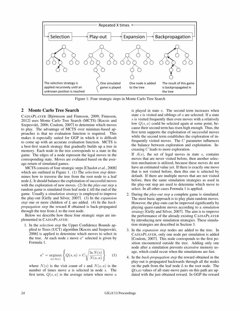
Repeated X times
Selection Play out Expansion Backpropagation
The selection strategy is
applied recursively until an
One node is added
to the tree
One simulated
game is played
The result of this game
is backpropagated inapplied recursively until an
unknown position is reached
to the treegame is played is backpropagated in
the tree
Figure 1: Four strategic steps in Monte Carlo Tree Search
2 Monte Carlo Tree SearchCADIAPLAYER [Bjornsson and Finnsson, 2009; Finnsson,2012] uses Monte Carlo Tree Search (MCTS) [Kocsis andSzepesvari, 2006; Coulom, 2007] to determine which movesto play. The advantage of MCTS over minimax-based ap-proaches is that no evaluation function is required. Thismakes it especially suited for GGP in which it is difficultto come up with an accurate evaluation function. MCTS isa best-first search strategy that gradually builds up a tree inmemory. Each node in the tree corresponds to a state in thegame. The edges of a node represent the legal moves in thecorresponding state. Moves are evaluated based on the aver-age return of simulated games.
MCTS consists of four strategic steps [Chaslot et al., 2008]which are outlined in Figure 1. (1) The selection step deter-mines how to traverse the tree from the root node to a leafnode L. It should balance the exploitation of successful moveswith the exploration of new moves. (2) In the play-out step arandom game is simulated from leaf node L till the end of thegame. Usually a simulation strategy is employed to improvethe play-out [Gelly and Silver, 2007]. (3) In the expansionstep one or more children of L are added. (4) In the back-propagation step the reward R obtained is back-propagatedthrough the tree from L to the root node.
Below we describe how these four strategic steps are im-plemented in CADIAPLAYER:
1. In the selection step the Upper Confidence Bounds ap-plied to Trees (UCT) algorithm [Kocsis and Szepesvari,2006] is applied to determine which moves to select inthe tree. At each node s move a∗ selected is given byFormula 1.
a∗ = argmaxa∈A(s)
Q(s, a) + C
√lnN(s)
N(s, a)
(1)
where N(s) is the visit count of s and N(s, a) is thenumber of times move a is selected in node s. Thefirst term, Q(s, a) is the average return when move a
is played in state s. The second term increases whenstate s is visited and siblings of a are selected. If a states is visited frequently then even moves with a relativelylow Q(s, a) could be selected again at some point, be-cause their second term has risen high enough. Thus, thefirst term supports the exploitation of successful moveswhile the second term establishes the exploration of in-frequently visited moves. The C parameter influencesthe balance between exploration and exploitation. In-creasing C leads to more exploration.If A(s), the set of legal moves in state s, containsmoves that are never visited before, then another selec-tion mechanism is utilized, because these moves do nothave an estimated value yet. If there is exactly one movethat is not visited before, then this one is selected bydefault. If there are multiple moves that are not visitedbefore, then the same simulation strategies as used inthe play-out step are used to determine which move toselect. In all other cases Formula 1 is applied.
2. During the play-out step a complete game is simulated.The most basic approach is to play plain random moves.However, the play-outs can be improved significantly byplaying quasi-random moves according to a simulationstrategy [Gelly and Silver, 2007]. The aim is to improvethe performance of the already existing CADIAPLAYERby introducing new simulation strategies. These simula-tion strategies are described in Section 3.
3. In the expansion step nodes are added to the tree. InCADIAPLAYER, only one node per simulation is added[Coulom, 2007]. This node corresponds to the first po-sition encountered outside the tree. Adding only onenode after a simulation prevents excessive memory us-age, which could occur when the simulations are fast.
4. In the back-propagation step the reward obtained in theplay-out is propagated backwards through all the nodeson the path from the leaf node L to the root node. TheQ(s,a) values of all state-move pairs on this path are up-dated with the just obtained reward. In GGP the reward
GIGA'13 Proceedings24
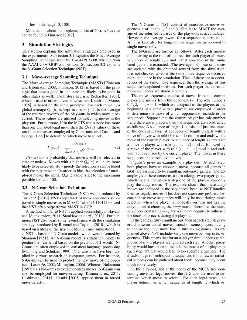
lies in the range [0, 100].
More details about the implementation of CADIAPLAYERcan be found in Finnsson [2012].
3 Simulation StrategiesThis section explains the simulation strategies employed inthe experiments. Subsection 3.1 explains the Move-AverageSampling Technique used by CADIAPLAYER when it wonthe AAAI 2008 GGP competition. Subsection 3.2 explainsthe N-Gram Selection Technique (NST).
3.1 Move-Average Sampling TechniqueThe Move-Average Sampling Technique (MAST) [Finnssonand Bjornsson, 2008; Finnsson, 2012] is based on the prin-ciple that moves good in one state are likely to be good inother states as well. The history heuristic [Schaeffer, 1983],which is used to order moves in αβ search [Knuth and Moore,1975], is based on the same principle. For each move a, aglobal average Qh(a) is kept in memory. It is the averageof the returned rewards of the play-outs in which move a oc-curred. These values are utilized for selecting moves in theplay-out. Furthermore, if in the MCTS tree a node has morethan one unvisited legal move then the Qh(a) values of theseunvisited moves are employed by Gibbs measure [Casella andGeorge, 1992] to determine which move to select:
P (s, a) =eQh(a)/τ∑
b∈A(s) eQh(b)/τ
(2)
P (s, a) is the probability that move a will be selected instate or node s. Moves with a higher Qh(a) value are morelikely to be selected. How greedy the selection is can be tunedwith the τ parameter. In order to bias the selection of unex-plored moves the initial Qh(a) value is set to the maximumpossible score of 100.
3.2 N-Gram Selection TechniqueThe N-Gram Selection Technique (NST) was introduced byTak et al. [2012]. NST keeps track of move sequences as op-posed to single moves as in MAST. Tak et al. [2012] showedthat NST often outperforms MAST in GGP.
A method similar to NST is applied successfully in Havan-nah [Stankiewicz, 2011; Stankiewicz et al., 2012]. Further-more, NST also bears some resemblance with the simulationstrategy introduced by Rimmel and Teytaud [2010], which isbased on a tiling of the space of Monte Carlo simulations.
NST is based on N-Gram models, which were invented byShannon [1951]. An N-Gram model is a statistical model topredict the next word based on the previous N-1 words. N-Grams are often employed in statistical language processing[Manning and Schutze, 1999]. N-Grams also have been ap-plied in various research on computer games. For instance,N-Grams can be used to predict the next move of the oppo-nent [Laramee, 2002; Millington, 2006]. Whereas, Nakamura[1997] uses N-Grams to extract opening moves. N-Grams canalso be employed for move ordering [Kimura et al., 2011;Hashimoto, 2011]. Otsuki [2005] applied them in forcedmove detection.
The N-Grams in NST consist of consecutive move se-quences z of length 1, 2 and 3. Similar to MAST the aver-age of the returned rewards of the play-outs is accumulated.However, the average reward for a sequence z, here calledR(z), is kept also for longer move sequences as opposed tosingle moves only.
The N-Grams are formed as follows. After each simula-tion, starting at the root of the tree, for each player all movesequences of length 1, 2 and 3 that appeared in the simu-lated game are extracted. The averages of these sequencesare updated with the obtained reward from the simulation.It is not checked whether the same move sequence occurredmore than once in the simulation. Thus, if there are m occur-rences of the same move sequence, then the average of thissequence is updated m times. For each player the extractedmove sequences are stored separately.
The move sequences consist of moves from the currentplayer and moves from the opponent(s). The role numbers0, 1, 2, · · · , n − 1, which are assigned to the players at thebeginning of a game with n players, are employed in orderto determine the move of which opponent to include in thesequences. Suppose that the current player has role numberi and there are n players, then the sequences are constructedas follows. A sequence of length 1 consists of just one moveof the current player. A sequence of length 2 starts with amove of player with role (i+ n− 1) mod n and ends with amove of the current player. A sequence of length 3 starts witha move of player with role (i+ n− 2) mod n, followed bya move of the player with role (i+ n− 1) mod n and endswith a move made by the current player. The moves in thesesequences are consecutive moves.
Figure 2 gives an example of a play-out. At each step,both players have to choose a move, because all games inGGP are assumed to be simultaneous-move games. The ex-ample given here concerns a turn-taking, two-player game,which means that at each step one of the players can onlyplay the noop move. The example shows that these noopmoves are included in the sequences, because NST handlesthem as regular moves. This does not cause any problem, be-cause these move sequences will only be used during moveselection when the player is not really on turn and has theonly option of choosing the noop move. Therefore, the movesequences containing noop moves do not negatively influencethe decision process during the play-out.
If the game is truly simultaneous, then at each step all play-ers choose an actual move instead of some players havingto choose the noop move like in turn-taking games. As ex-plained above, NST includes only one move per step in its se-quences. This means that for an n-player simultaneous game,moves of n− 1 players are ignored each step. Another possi-bility would have been to include the moves of all players ateach step, but that would lead to too specific sequences. Thedisadvantage of such specific sequences is that fewer statisti-cal samples can be gathered about them, because they occurmuch more rarely.
In the play-out, and at the nodes of the MCTS tree con-taining unvisited legal moves, the N-Grams are used to de-termine which move to select. For each legal move, theplayer determines which sequence of length 1, which se-
GIGA'13 Proceedings 25
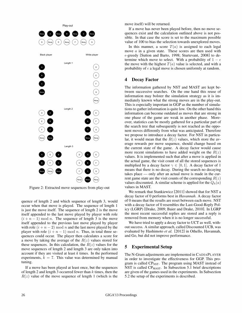
Figure 2: Extracted move sequences from play-out
quence of length 2 and which sequence of length 3, wouldoccur when that move is played. The sequence of length 1is just the move itself. The sequence of length 2 is the moveitself appended to the last move played by player with role(i+ n− 1) mod n. The sequence of length 3 is the moveitself appended to the previous last move played by playerwith role (i+ n− 2) mod n and the last move played by theplayer with role (i+ n− 1) mod n. Thus, in total three se-quences could occur. The player then calculates a score fora move by taking the average of the R(z) values stored forthese sequences. In this calculation, the R(z) values for themove sequences of length 2 and length 3 are only taken intoaccount if they are visited at least k times. In the performedexperiments, k = 7. This value was determined by manualtuning.
If a move has been played at least once, but the sequencesof length 2 and length 3 occurred fewer than k times, then theR(z) value of the move sequence of length 1 (which is the
move itself) will be returned.If a move has never been played before, then no move se-
quences exist and the calculation outlined above is not pos-sible. In that case the score is set to the maximum possiblevalue of 100 to bias the selection towards unexplored moves.
In this manner, a score T (a) is assigned to each legalmove a in a given state. These scores are then used withϵ-greedy [Sutton and Barto, 1998; Sturtevant, 2008] to de-termine which move to select. With a probability of 1 − ϵthe move with the highest T (a) value is selected, and with aprobability of ϵ a legal move is chosen uniformly at random.
4 Decay FactorThe information gathered by NST and MAST are kept be-tween successive searches. On the one hand this reuse ofinformation may bolster the simulation strategy as it is im-mediately known what the strong moves are in the play-out.This is especially important in GGP as the number of simula-tions to gather information is quite low. On the other hand thisinformation can become outdated as moves that are strong inone phase of the game are weak in another phase. More-over, statistics can be mostly gathered for a particular part ofthe search tree that subsequently is not reached as the oppo-nent moves differently from what was anticipated. Thereforewe propose to introduce a decay factor. For NST in particu-lar, it would mean that the R(z) values, which store the av-erage rewards per move sequence, should change based onthe current state of the game. A decay factor would causemore recent simulations to have added weight on the R(z)values. It is implemented such that after a move is applied inthe actual game, the visit count of all the stored sequences ismultiplied by a decay factor γ ∈ [0, 1]. A decay factor of 1means that there is no decay. During the search no decayingtakes place — only after an actual move is made in the cur-rent game state are the visit counts of the corresponding R(z)values discounted. A similar scheme is applied for the Qh(a)values in MAST.
We remark that Stankiewicz [2011] showed that for NST adecay factor of 0 performs best in Havannah. A decay factorof 0 means that the results are reset between each move. NSTwith a decay factor of 0 resembles the Last-Good-Reply Pol-icy (LGRP) [Drake, 2009; Baier and Drake, 2010]. In LGRPthe most recent successful replies are stored and a reply isremoved from memory when it is no longer successful.
We have tried to apply a decay factor to UCT as well, with-out success. A similar approach, called Discounted UCB, wasevaluated by Hashimoto et al. [2012] in Othello, Havannah,and Go, but did not improve performance.
5 Experimental SetupThe N-Gram adjustments are implemented in CADIAPLAYERin order to investigate the effectiveness for GGP. This pro-gram is called CPNST. The program using MAST instead ofNST is called CPMAST. In Subsection 5.1 brief descriptionsare given of the games used in the experiments. In Subsection5.2 the setup of the experiments is described.
GIGA'13 Proceedings26

5.1 GamesBelow an overview is given of the games used in the exper-iments. Note that most of the classic games enlisted beloware usually a variant of its original counterpart. The mostcommon adjustments are a smaller board size and a bound onthe number of steps. The following two-player, turn-takinggames are used:
• Zhadu is a strategy game consisting of a placementphase and a movement phase. The first piece that is cap-tured, determines what other piece need to be capturedin order to win.
• In GridGame each player has to find a book, a candleand a bell. A score between 0 and 100 is given, based onhow many items where found.
• 3DTicTacToe is a variant on Tic-Tac-Toe. It is played ona 4×4×4 cube and the goal is to align four pieces in astraight line.
• TTCC4 stands for: TicTacChessCheckersFour. Eachplayer has a pawn, a checkers piece and a knight. Theaim of each player is to form a line of three with its ownpieces.
• Connect5 is played on an 8×8 board and the player onturn has to place a piece in an empty square. The aimis to place five consecutive pieces of the own color hori-zontally, vertically or diagonally, like Five-in-a-Row.
• Checkers is played on an 8×8 board and the aim is tocapture pieces of the opponent.
• Breakthrough is played on an 8×8 board. Each playerstarts on one side of the board and the goal is to moveone of their pieces to the other side of the board.
• Knightthrough is almost the same as Breakthrough, butis played with chess knights.
• Othello is played on an 8×8 board. Each turn a playerplaces a piece of its own color on the board. This willchange the color of some of the pieces of the opponent.The aim is to have the most pieces of the own color onthe board at the end of the game.
• Skirmish is played on an 8×8 board with different kindof pieces, namely: bishops, pawns, knights and rooks.The aim is to capture as many pieces from the opponentas possible, without losing to many pieces either.
• Merrills is also known as Nine Men’s Morris. Both play-ers start with nine pieces each. In order to win, piecesof the opponent need to be captured. The objective is toform a horizontal or vertical line of three pieces, calleda mill, because pieces in a mill cannot be captured. Thegame ends when one player has only two pieces left.
• Quad is played on a 7×7 board. Each player has ‘quad’pieces and ‘white’ pieces. The purpose of the ‘white’pieces is to form blockades. The player that forms asquare consisting of four ‘quad’ pieces wins the game.
• Sheep and Wolf is an asymmetrical game played on an8×8 board. One player controls the Sheep and the otherplayer controls the Wolf. The game ends when none of
the players can move or when the Wolf is behind theSheep. In this case, if the Wolf is not able to move theSheep wins. Otherwise, the Wolf wins.
The following three-player, turn-taking games are used:
• Farmers is a trading game. In the beginning of the game,each player gets the same amount of money. They canuse the money to buy cotton, cloth, wheat and floor. Itis also possible to buy a farm or factory and then theplayer can produce its own products. The player that hasthe most money at the end of the game wins.
• TTCC43P is the same as TTCC4, but then with one extraplayer.
• Chinese Checkers 3P is played on a star shaped board.Each player starts with three pieces positioned in onecorner. The aim is to move all these three pieces to theempty corner at the opposite side of the board. This isa variant of the original Chinese Checkers, because ac-cording to the standard rules each player has ten piecesinstead of three.
The following two-player, simultaneous-move games areused:
• Battle is played on an 8×8 board. Each player has 20disks. These disks can move one square or capture anopponent square next to them. Instead of a move, theplayer can choose to defend a square occupied by theirpiece. If an attacker attacks such a defended square,the attacker will be captured. The goal is to be the firstplayer to capture 10 opponent disk.
• Chinook is a variant of Breakthrough where two inde-pendent games are played simultaneously. One game onthe white squares and another one on the black squares.Black and White move their pieces simultaneously likeCheckers pawns. As in Breakthrough, the first playerthat reaches the opposite side of the board wins thegame.
• In Runners each turn both players decide how manysteps they want to move forward or backward. The aimis to reach the goal location before the opponent does.
• Pawn Whopping is similar to Breakthrough, but withslightly different movement and is simultaneous.
These games were chosen because they are used in sev-eral previous CADIAPLAYER experiments [Finnsson, 2007;Finnsson and Bjornsson, 2008; 2009; Bjornsson and Finns-son, 2009; Finnsson and Bjornsson, 2010; 2011; Finnsson,2012]. Pawn Whopping was used during the German Openin GGP of 2011 [Kissmann and Federholzner, 2011]. Fur-thermore, this selection contains different types of games.Namely, two-player games, multi-player games, constant-sum games and general-sum games (e.g. GridGame, Skir-mish, Battle, Chinook, Farmers and ChineseCheckers3P).
5.2 SetupIn all experiments two variants of CADIAPLAYER arematched against each other. The ϵ and k parameters of theNST simulation strategy are set to 0.2 and 7, respectively.
GIGA'13 Proceedings 27

Table 1: Win % of CPNST with different values of γ against CPNST with γ = 1, startclock=60s, playclock=30s.Game γ = 0 γ = 0.2 γ = 0.4 γ = 0.6 γ = 0.8
Zhadu 26.6 (±3.75) 32.4 (±4.05) 36.5 (±3.80) 47.0 (±3.67) 47.4 (±4.97)GridGame 49.4 (±5.38) 49.9 (±3.43) 50.5 (±4.11) 49.8 (±3.43) 49.3 (±4.58)
3DTicTacToe 66.5 (±4.97) 69.0(±3.53) 66.2 (±4.29) 61.8 (±4.82) 58.2 (±4.85)TTCC4 27.5 (±4.75) 44.4 (±5.04) 47.9 (±4.51) 52.5 (±5.63) 51.7 (±4.33)
Connect5 61.1 (±4.72) 69.1 (±4.19) 65.7 (±4.02) 66.2 (±3.69) 59.4 (±4.99)Checkers 45.6 (±4.76) 54.0 (±4.72) 63.3 (±4.41) 60.8 (±5.38) 62.6 (±5.46)
Breakthrough 37.3 (±5.22) 41.9 (±4.36) 45.5 (±4.25) 44.6 (±5.18) 53.6 (±5.62)Knightthrough 46.4 (±5.62) 38.1 (±4.95) 43.6 (±4.64) 44.1 (±5.58) 54.6 (±5.60)
Othello 36.1 (±5.29) 44.4 (±4.17) 45.2 (±4.02) 49.1 (±5.46) 48.1 (±5.58)Skirmish 51.0 (±5.28) 49.1 (±5.28) 53.2 (±4.85) 55.1 (±4.40) 52.2 (±4.48)Merrills 58.3 (±4.32) 58.6 (±5.05) 58.3 (±3.89) 60.7 (±5.02) 55.6 (±5.22)
Quad 61.5 (±3.87) 68.7 (±3.63) 67.2 (±3.37) 65.3 (±3.11) 60.4 (±4.25)Sheep and Wolf 44.3 (±4.11) 44.0 (±3.41) 47.2 (±4.08) 49.0 (±3.46) 52.2 (±5.47)
Farmers 44.9 (±4.11) 52.7 (±2.62) 53.0 (±3.13) 50.3 (±2.62) 50.3 (±4.10)TTCC43P 53.2 (±5.65) 56.2 (±4.31) 54.6 (±3.96) 54.5 (±3.59) 56.2 (±5.61)
ChineseCheckers3P 41.4 (±5.09) 50.7 (±4.24) 53.2 (±4.67) 51.3 (±4.29) 51.0 (±5.66)Battle 56.6 (±5.32) 65.6 (±4.46) 63.8 (±4.15) 64.5 (±5.03) 59.3 (±5.15)
Chinook 45.7 (±5.30) 55.0 (±4.75) 57.3 (±4.36) 56.9 (±5.31) 54.4 (±5.36)Runners 55.8 (±4.73) 53.4 (±4.66) 49.7 (±4.66) 49.5 (±4.67) 52.1 (±3.98)
Pawn Whopping 47.2 (±2.72) 50.2 (±2.72) 51.5 (±2.71) 50.0 (±2.71) 50.3 (±2.30)
Their values were determined by manual tuning. The τ pa-rameter of the Gibbs measure used in CADIAPLAYER wasleft unchanged to its preset value of 10. The program usingNST cuts off simulations that take more than 400 moves. Theprogram using MAST does not cut off.
In the experiments two different time settings are used.When tuning γ the startclock is set to 60s and the playclockis set to 30s. In the validation experiments, the startclock isset to 70s and the playclock is set to 40s. Different time set-tings are used, because on the one hand we want to have ahigh number of simulations per move, but on the other handit takes much computation time to tune γ.
In all experiments, the programs switch roles such thatno one has any advantage. For the two-player games, thereare two possible configurations. For the three-player games,there are eight possible configurations, where two of themconsist of three times the same player. Therefore, only sixconfigurations are employed in the experiments [Sturtevant,2008]. All experiments are performed on a computer consist-ing of 64 AMD Opteron 2.2 Ghz cores.
6 Experimental ResultsIn the experiments it is examined how different decay fac-tors perform. The original N-Gram player, CPNST, is matchedagainst CPNST with a decay factor. After determining the bestdecay factor, CPNST is matched against CPMAST to further val-idate whether the decay factor is a genuine improvement. Fi-nally, CPMAST with a decay factor is matched against CPNSTto investigate whether decaying is beneficial for MAST aswell. All tables show both a win rate, averaged over at least300 games, and a 95% confidence interval. The win rate iscalculated as follows. For the two-player games, each gamewon gives a score of 1 point and each game that ends in adraw results in a score of 1
2 point. The win rate is the sumof these points divided by the total number of games played.For the three-player games, a similar calculation is performed
except the draws are counted differently. If all three playersobtained the same reward, then the draw is counted as 1
3 point.If two players obtained the same, highest reward, the draw iscounted as 1
2 point for the corresponding players.
Table 2: Win % of CPNST with γ ∈ 1; 0.6 against CPMASTwith γ = 1, startclock=70s, playclock=40s
Game γ = 1 γ = 0.6
Zhadu 74.9 (±4.51) 75.5 (±4.39)GridGame 52.3 (±3.79) 52.8 (±4.52)
3DTicTacToe 73.3 (±3.87) 80.4 (±3.59)TTCC4 85.4 (±2.18) 84.4 (±1.69)
Connect5 70.4 (±3.57) 78.9 (±3.79)Checkers 68.9 (±5.14) 80.0 (±4.38)
Breakthrough 63.7 (±3.69) 72.3 (±2.82)Knightthrough 47.7 (±5.29) 50.0 (±5.30)
Othello 67.4 (±4.54) 67.0 (±4.55)Skirmish 69.6 (±5.01) 70.1 (±5.03)Merrills 44.6 (±2.81) 50.9 (±2.82)
Quad 79.1 (±2.96) 92.3 (±2.30)Sheep and Wolf 61.1 (±3.94) 61.3 (±4.73)
Farmers 72.2 (±2.64) 73.1 (±3.11)TTCC43P 53.2 (±3.66) 58.1 (±2.43)
ChineseCheckers3P 57.6 (±4.87) 55.1 (±5.32)Battle 19.2 (±4.01) 29.8 (±4.69)
Chinook 73.7 (±2.88) 79.4 (±1.96)Runners 35.7 (±4.62) 36.7 (±4.60)
Pawn Whopping 52.2 (±2.80) 51.3 (±2.80)
6.1 Decay Factor in NSTTable 1 shows the win rate of CPNST with decay versus CPNSTwithout decay. Note that no decay means that γ = 1. Thewin rates in bold indicate that they are the highest win rateof their row. The results show that decay may improve theprogram. Furthermore, the results demonstrate that simplyresetting the NST statistics each move (which means γ = 0)can decrease the performance significantly in some games
GIGA'13 Proceedings28
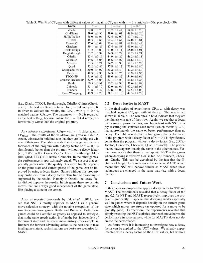
Table 3: Win % of CPMAST with different values of γ against CPMAST with γ = 1, startclock=60s, playclock=30sGame γ = 0 γ = 0.2 γ = 0.6
Zhadu 52.8 (±3.73) 51.2 (±4.44) 54.2 (±3.78)GridGame 50.0 (±3.56) 50.0 (±4.01) 49.9 (±3.26)
3DTicTacToe 88.0 (±1.95) 92.4 (±2.00) 87.7 (±2.10)TTCC4 48.3 (±3.65) 50.4 (±4.54) 52.0 (±3.81)
Connect5 77.6 (±3.04) 76.4 (±3.81) 68.8 (±3.44)Checkers 59.1 (±4.43) 67.4 (±4.58) 65.0 (±4.45)
Breakthrough 53.2 (±5.03) 53.0 (±4.11) 58.0 (±4.91)Knightthrough 53.2 (±3.92) 54.3 (±3.22) 52.2 (±4.21)
Othello 43.4 (±5.13) 44.9 (±4.22) 46.2 (±5.11)Skirmish 49.6 (±4.08) 48.6 (±5.22) 51.6 (±4.40)Merrills 53.5 (±3.71) 54.7 (±3.98) 52.1 (±5.23)
Quad 72.2 (±2.86) 77.8 (±3.17) 73.9 (±2.80)Sheep and Wolf 50.0 (±3.92) 51.2 (±4.40) 49.2 (±3.59)
Farmers 48.3 (±2.90) 54.3 (±3.25) 53.9 (±4.95)TTCC43P 51.9 (±3.37) 49.6 (±4.37) 54.0 (±3.64)
ChineseCheckers3P 52.9 (±4.06) 53.1 (±5.20) 51.8 (±4.36)Battle 50.5 (±3.57) 50.2 (±2.93) 52.6 (±3.82)
Chinook 53.1 (±3.70) 62.0 (±4.64) 60.2 (±3.95)Runners 51.8 (±4.42) 53.8 (±5.03) 52.5 (±4.08)
Pawn Whopping 49.9 (±2.78) 50.1 (±3.13) 49.5 (±4.78)
(i.e., Zhadu, TTCC4, Breakthrough, Othello, ChineseCheck-ers3P). The best results are obtained for γ = 0.4 and γ = 0.6.In order to validate the results, the CPNST with γ = 0.6 ismatched against CPMAST. The parameter γ = 0.6 is regardedas the best setting, because unlike for γ = 0.4 it never per-forms really worse than the original program.
As a reference experiment, CPNST with γ = 1 plays againstCPMAST. The results of the validation are given in Table 2.Again, win rates in bold indicate that they are the highest winrate of their row. The table reveals that in nine games the per-formance of the program with a decay factor of γ = 0.6 issignificantly better than the program without a decay factor(i.e., 3DTicTacToe, Connect5, Checkers, Breakthrough, Mer-rills, Quad, TTCC43P, Battle, Chinook). In the other games,the performance is approximately equal. We suspect that es-pecially games where the quality of a move highly dependson the game state and current phase of the game, can be im-proved by using a decay factor. Games without this propertymay profit less from a decay factor. This line of reasoning issupported by the results. Namely in Othello the decay fac-tor did not improve the results. In this game there are certainmoves that are always good independent of the game state,like placing a stone in the corner.
Also, as reported previously by Tak et al. [2012], wesee that NST is mostly superior to MAST as a generalmove-selection strategy, with the notable exceptions of thesimultaneous-move games Battle and Runners. Both thesegames could be classified as greedy as opposed to strategic,that is, the same greedy action is often the best independent ofthe current state and the recent move history (for example, inRunners the furthest advancing action is the best one to takein all game states); such situations are best-case scenarios forMAST.
6.2 Decay Factor in MASTIn the final series of experiments CPMAST with decay wasmatched against CPMAST without decay. The results areshown in Table 3. The win rates in bold indicate that they arethe highest win rate of their row. Again, we see that a decayfactor may improve the program. In contrast with NST, sim-ply resetting the statistics each move (which means γ = 0)has approximately the same or better performance than nodecay. The table reveals that in five games the performanceof the program with a decay factor of γ = 0.2 is significantlybetter than the program without a decay factor (i.e., 3DTic-TacToe, Connect5, Checkers, Quad, Chinook). The perfor-mance stays approximately the same in the other games. Fur-thermore, notice that there is overlap with NST in the gameswhere decaying is effective (3DTicTacToe, Connect5, Check-ers, Quad). This can be explained by the fact that the N-Grams of length 1 are in essence the same as MAST, whichmeans that NST will behave similar as MAST when thesetechniques are changed in the same way (e.g with a decayfactor).
7 Conclusions and Future WorkIn this paper we proposed to apply a decay factor to NST andMAST. The experiments revealed that a decay factor of 0.6and 0.2 for NST and MAST, respectively, improves the pro-gram significantly. It appears that decaying works especiallywell in games where it depends heavily on the current gamestate which moves are strong (as opposed for a move to beglobally good). Furthermore, the experiments revealed thatsimply resetting the NST statistics after each move harms theperformance in some games, while for MAST it does not de-crease the performance.
As future work it is interesting to investigate how a decayfactor can be applied to the UCT values. We already exper-imented with a decay factor on the UCT values, but without
GIGA'13 Proceedings 29
success so far. Also of interest is to find out whether there areother methods that can be used to decay the UCT values suc-cessfully. Related work is the Discounted UCB, but this wasalso unsuccessful [Hashimoto et al., 2012]. Another directionof future work would be to investigate whether a decay factoralso works within the search iself.
AcknowledgementsThis work is funded by the Netherlands Organisation for ScientificResearch (NWO) in the framework of the project GoGeneral, grantnumber 612.001.121.
References[Baier and Drake, 2010] H. Baier and P.D. Drake. The Power of Forgetting: Improving
the Last-Good-Reply Policy in Monte Carlo Go. IEEE Transactions on Computa-tional Intelligence and AI in Games, 2(4):303 –309, 2010.
[Bjornsson and Finnsson, 2009] Y. Bjornsson and H. Finnsson. CadiaPlayer: ASimulation-Based General Game Player. IEEE Transactions on Computational In-telligence and AI in Games, 1(1):4 –15, 2009.
[Casella and George, 1992] G. Casella and E.I. George. Explaining the Gibbs Sampler.The American Statistician, 46(3):167–174, 1992.
[Chaslot et al., 2008] G.M.J.-B. Chaslot, M.H.M. Winands, J.W.H.M. Uiterwijk, H.J.van den Herik, and B. Bouzy. Progressive Strategies for Monte-Carlo Tree Search.New Mathematics and Natural Computation, 4(3):343–357, 2008.
[Clune, 2007] J. Clune. Heuristic Evaluation Functions for General Game Playing. InProceedings of the Twenty-Second AAAI Conference on Artificial Intelligence, pages1134–1139, Menlo Park, California, 2007. The AAAI Press.
[Coulom, 2007] R. Coulom. Efficient Selectivity and Backup Operators in Monte-Carlo Tree Search. In H.J. van den Herik, P. Ciancarini, and H.H.L.M. Donkers,editors, CG 2006, volume 4630 of LNCS, pages 72–83, Berlin-Heidelberg, Germany,2007. Springer-Verlag.
[Drake, 2009] P. Drake. The Last-Good-Reply Policy for Monte-Carlo Go. ICGAJournal, 32(4):221–227, 2009.
[Finnsson and Bjornsson, 2008] H. Finnsson and Y. Bjornsson. Simulation-Based Ap-proach to General Game Playing. In D. Fox and C.P. Gomes, editors, Proceedings ofthe Twenty-Third AAAI Conference on Artificial Intelligence, pages 259–264, MenloPark, California, 2008. AAAI Press.
[Finnsson and Bjornsson, 2009] H. Finnsson and Y. Bjornsson. Simulation Control inGeneral Game Playing Agents. In The IJCAI Workshop on General Game Playing(GIGA’09), pages 21–26, Pasadena, California, 2009.
[Finnsson and Bjornsson, 2010] H. Finnsson and Y. Bjornsson. Learning SimulationControl in General Game-Playing Agents. In M. Fox and D. Poole, editors, Pro-ceedings of the Twenty-Fourth AAAI Conference on Artificial Intelligence, pages954–959, Menlo Park, California, 2010. AAAI Press.
[Finnsson and Bjornsson, 2011] H. Finnsson and Y. Bjornsson. CadiaPlayer: SearchControl Techniques. KI Journal, 25(1):9–16, 2011.
[Finnsson, 2007] H. Finnsson. CADIA-Player: A General Game Playing Agent. Mas-ter’s thesis, School of Computer Science, Reykjavık University, Reykjavık, Iceland,2007.
[Finnsson, 2012] H. Finnsson. Simulation-Based General Game Playing. PhD thesis,School of Computer Science, Reykjavık University, Reykjavık, Iceland, 2012.
[Gelly and Silver, 2007] S. Gelly and D. Silver. Combining Online and Offline Knowl-edge in UCT. In Z. Ghahramani, editor, Proceedings of the 24th International Con-ference on Machine Learning, ICML ’07, pages 273–280, New York, New York,2007. ACM.
[Hashimoto et al., 2012] J. Hashimoto, A. Kishimoto, K. Yoshizoe, and K. Ikeda. Ac-celerated UCT and Its Application to Two-Player Games. In H.J. van den Herik andA. Plaat, editors, Advances in Computer Games, volume 7168 of LNCS, pages 1–12,Berlin-Heidelberg, Germany, 2012. Springer-Verlag.
[Hashimoto, 2011] J. Hashimoto. A Study on Game-Independent Heuristics in Game-Tree Search. PhD thesis, School of Information Science, Japan Advanced Instituteof Science and Technology, Kanazawa, Japan, 2011.
[Kimura et al., 2011] T. Kimura, T. Ugajin, and Y. Kotani. Bigram Realization Proba-bility for Game Tree Search. In 2011 International Conference on Technologies andApplications of Artificial Intelligence (TAAI), pages 260–265, 2011.
[Kissmann and Federholzner, 2011] P. Kissmann and T. Federholzner. German Openin GGP 2011, 2011. http://www.tzi.de/∼kissmann/ggp/go-ggp/classical/games/.
[Knuth and Moore, 1975] D.E. Knuth and R.W. Moore. An Analysis of Alpha-BetaPruning. Artificial Intelligence, 6(4):293 – 326, 1975.
[Kocsis and Szepesvari, 2006] L. Kocsis and C. Szepesvari. Bandit Based Monte-Carlo Planning. In J. Furnkranz, T. Scheffer, and M. Spiliopoulou, editors, Proceed-ings of the EMCL 2006, volume 4212 of LNCS, pages 282–293, Berlin-Heidelberg,Germany, 2006. Springer-Verlag.
[Kozelek, 2009] T. Kozelek. Methods of MCTS and the Game Arimaa. Master’s the-sis, Department of Theoretical Computer Science and Mathematical Logic, CharlesUniversity, Prague, Czech Republic, 2009.
[Laramee, 2002] F.D. Laramee. Using N-Gram Statistical Models to Predict PlayerBehavior. In S. Rabin, editor, AI Programming Wisdom, volume 1, chapter 11,pages 596–601. Charles River Media, 2002.
[Manning and Schutze, 1999] C.D. Manning and H. Schutze. Foundations of Statisti-cal Natural Language Processing. The MIT Press, USA, 1999.
[Mehat and Cazenave, 2010] J. Mehat and T. Cazenave. Ary, a General Game PlayingProgram. In XIIIth Board Games Studies Colloquium, Paris, France, 2010.
[Millington, 2006] I. Millington. Artificial Intelligence for Games, chapter 7, pages580–591. Morgan Kaufmann, first edition, 2006.
[Nakamura, 1997] T. Nakamura. Acquisition of Move Sequence Patterns from GameRecord Database Using N-gram Statistics. In Proceedings of the 4th Game Pro-gramming Workshop in Japan, pages 96–105, 1997.
[Otsuki, 2005] T. Otsuki. Extraction of ‘Forced Move’ from N-Gram Statistics. In Pro-ceedings of the 10th Game Programming Workshop in Japan, pages 89–96, 2005.
[Rimmel and Teytaud, 2010] A. Rimmel and F. Teytaud. Multiple Overlapping Tilesfor Contextual Monte Carlo Tree Search. In C. Di Chio, S. Cagnoni, C. Cotta,M. Ebner, A. Ekart, A. Esparcia-Alcazar, C-K. Goh, J. Merelo, F. Neri, M. Preuß,J. Togelius, and G. Yannakakis, editors, Applications of Evolutionary Computa-tion, volume 6024 of LNCS, pages 201–210, Berlin-Heidelberg, Germany, 2010.Springer-Verlag.
[Schaeffer, 1983] J. Schaeffer. The History Heuristic. ICCA Journal, 6(3):16–19,1983.
[Schiffel and Thielscher, 2007a] S. Schiffel and M. Thielscher. Automatic Construc-tion of a Heuristic Search Function for General Game Playing. In Seventh IJCAIInternational Workshop on Nonmontonic Reasoning, Action and Change (NRAC07),2007.
[Schiffel and Thielscher, 2007b] S. Schiffel and M. Thielscher. Fluxplayer: A Suc-cessful General Game Player. In Proceedings of the Twenty-Second AAAI Confer-ence on Artificial Intelligence, pages 1191–1196, Menlo Park, California, 2007. TheAAAI Press.
[Shannon, 1951] C.E. Shannon. Prediction and Entropy of Printed English. The BellSystem Technical Journal, 30(1):50–64, 1951.
[Stankiewicz et al., 2012] J.A. Stankiewicz, M.H.M. Winands, and J.W.H.M. Uiter-wijk. Monte-Carlo Tree Search Enhancements for Havannah. In H.J. van den Herikand A. Plaat, editors, Advances in Computer Games (ACG 13), volume 7168 ofLNCS, pages 60–71, Berlin-Heidelberg, Germany, 2012. Springer-Verlag.
[Stankiewicz, 2011] J.A. Stankiewicz. Knowledge-Based Monte-Carlo Tree Searchin Havannah. Master’s thesis, Department of Knowledge Engineering, MaastrichtUniversity, Maastricht, The Netherlands, 2011.
[Sturtevant, 2008] N.R. Sturtevant. An Analysis of UCT in Multi-player Games. ICGAJournal, 31(4):195–208, 2008.
[Sutton and Barto, 1998] R.S. Sutton and A.G. Barto. Reinforcement Learning: AnIntroduction. Adaptive Computation and Machine Learning. The MIT Press, Cam-bridge, Massachusetts, 1998.
[Tak et al., 2012] M.J.W. Tak, M.H.M. Winands, and Y. Bjornsson. N-Grams and theLast-Good-Reply Policy Applied in General Game Playing. IEEE Transactions onComputational Intelligence and AI in Games, 4(2):73–83, 2012.
GIGA'13 Proceedings30
High Speed Forward Chaining for General Game PlayingMichael Schofield
CSE, The University of New South Wales, Sydney, [email protected]
Abdallah SaffidineLAMSADE, Universite Paris-Dauphine, Paris, France
AbstractGeneral Game Playing demands that an AI systembe capable of interpreting a set of rules for a previ-ously unseen game and reason about the game stateas efficiently as possible. In simulation based rea-soners, the number of states that can be visited ina fixed time limit is paramount. One technique forcalculating each game state is Forward Chaining;where the system calculates all of the relations thatcan be calculated from the current state and usesthat as a basis for the next state.In this work we progress some earlier work on For-ward Chaining and propose two additional features.Firstly the augmentation of rule processing usingreference tables to facilitate high speed instantia-tion of ground relations into a rule, and secondlyan empirical hypothesis ordering strategy utilisingdata collected from the operation of the system tooptimise its performance. This paper proposes anddefines these additional features and presents ex-perimental data to support their use.
1 IntroductionMost General Game Playing (GGP) programs can be decom-posed into a rule engine and a search engine. The formerprocesses the rules of the game to determine which actionsare possible, which game states are terminal, and what the as-sociated utility for each player is. The search engine uses thisinformation together with some tree search algorithms suchas variants of A*, alpha-beta, or Monte Carlo Tree Search todecide what action to perform next.
The larger the explored state space, the more informed andbetter the submitted decisions. However, GGP competitionsrequire that playing programs submit an action within a spe-cific time, say 30 seconds. As a result, the strength of a play-ing program crucially depends on the speed of the rule engineand that of the search engine. Given that all state-of-the-art al-gorithms for search in GGP are data-intensive, the speed bot-tleneck lies on the side of the rule engine. These algorithmsinclude Monte Carlo Tree Search [Finnsson and Bjornsson,2008], Nested Monte Carlo Search [Mehat and Cazenave,2010], as well as depth-first search [Schiffel and Thielscher,
2007] in the classical track of the GGP competition. In theImperfect Information track, the Perfect Information MonteCarlo Sampling approach [Long et al., 2010; Schofield et al.,2012] puts even more stress on the rule engine.
A popular measure of raw speed performance of rule en-gine is the number of random simulations (so-called playouts)the engine can generate in given game in a second. As ex-ample of the large gap between domain specific engines andGGP engine, one can observe that an optimized program for19 × 19 Go can perform millions of simulations per secondswhile typical GGP program perform much less than 1000simuations per seconds on 7×6 Connect Four, a much shorterand simpler game [Saffidine and Cazenave, 2011].
Several approaches have been put forward to process gamerules written in the Game Description Language (GDL). Theclassic approach is to use a Prolog engine such as YAP [Costaet al., 2006] to interpret the rules. To this end, a syntactictranslation from GDL to Prolog is almost sufficient. Whilethe speed of the resulting engine is far from ideal, the easy set-up makes this approach the most popular one by far amongcompetition programs.
A similar but more involved approach is to compile GDLrules to a lower-level language such as C++ or Java so thatthe resulting program will simulate Prolog’s SLD resolu-tion [Waugh, 2009; Moller et al., 2011]. This SLD compi-lation approach leads to programs that are up to an order ofmagnitude faster than with the classic approach. However,practical use of such a model is hindered by the fact that ac-tual implementations do not handle the full range of the GameDescription Language, and in particular nested function con-stants are typically not supported.
Grounding the rules refers to the process of transforminga game description involving variables into a an equivalentdescription where variables have been replaced by possibleinstantiations. Not only is grounding the game rules neces-sary to apply answer-set programming techniques for solvingsingle agent games [Thielscher, 2009], but a ground descrip-tion is often faster to execute and interpret with SLD resolu-tion than the corresponding original description. In particu-lar, propositional automata can be used when the descriptionis ground [Cox et al., 2009]. The main problem with this ap-proach is that it can lead to an exponential blow-up in the sizeof the description. Most engines based on grounding fall backto a classic prolog interpreter when the game is too large to
GIGA'13 Proceedings 31
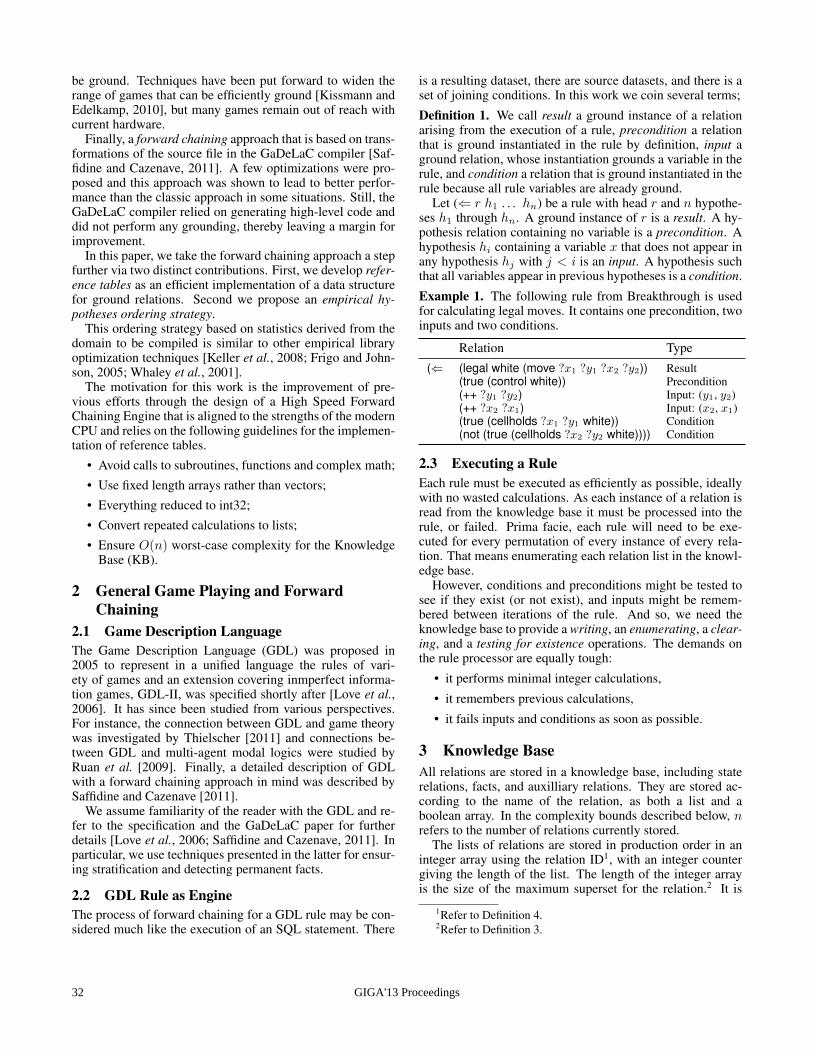
be ground. Techniques have been put forward to widen therange of games that can be efficiently ground [Kissmann andEdelkamp, 2010], but many games remain out of reach withcurrent hardware.
Finally, a forward chaining approach that is based on trans-formations of the source file in the GaDeLaC compiler [Saf-fidine and Cazenave, 2011]. A few optimizations were pro-posed and this approach was shown to lead to better perfor-mance than the classic approach in some situations. Still, theGaDeLaC compiler relied on generating high-level code anddid not perform any grounding, thereby leaving a margin forimprovement.
In this paper, we take the forward chaining approach a stepfurther via two distinct contributions. First, we develop refer-ence tables as an efficient implementation of a data structurefor ground relations. Second we propose an empirical hy-potheses ordering strategy.
This ordering strategy based on statistics derived from thedomain to be compiled is similar to other empirical libraryoptimization techniques [Keller et al., 2008; Frigo and John-son, 2005; Whaley et al., 2001].
The motivation for this work is the improvement of pre-vious efforts through the design of a High Speed ForwardChaining Engine that is aligned to the strengths of the modernCPU and relies on the following guidelines for the implemen-tation of reference tables.
• Avoid calls to subroutines, functions and complex math;
• Use fixed length arrays rather than vectors;
• Everything reduced to int32;
• Convert repeated calculations to lists;
• Ensure O(n) worst-case complexity for the KnowledgeBase (KB).
2 General Game Playing and ForwardChaining
2.1 Game Description LanguageThe Game Description Language (GDL) was proposed in2005 to represent in a unified language the rules of vari-ety of games and an extension covering inmperfect informa-tion games, GDL-II, was specified shortly after [Love et al.,2006]. It has since been studied from various perspectives.For instance, the connection between GDL and game theorywas investigated by Thielscher [2011] and connections be-tween GDL and multi-agent modal logics were studied byRuan et al. [2009]. Finally, a detailed description of GDLwith a forward chaining approach in mind was described bySaffidine and Cazenave [2011].
We assume familiarity of the reader with the GDL and re-fer to the specification and the GaDeLaC paper for furtherdetails [Love et al., 2006; Saffidine and Cazenave, 2011]. Inparticular, we use techniques presented in the latter for ensur-ing stratification and detecting permanent facts.
2.2 GDL Rule as EngineThe process of forward chaining for a GDL rule may be con-sidered much like the execution of an SQL statement. There
is a resulting dataset, there are source datasets, and there is aset of joining conditions. In this work we coin several terms;
Definition 1. We call result a ground instance of a relationarising from the execution of a rule, precondition a relationthat is ground instantiated in the rule by definition, input aground relation, whose instantiation grounds a variable in therule, and condition a relation that is ground instantiated in therule because all rule variables are already ground.
Let (⇐ r h1 . . . hn) be a rule with head r and n hypothe-ses h1 through hn. A ground instance of r is a result. A hy-pothesis relation containing no variable is a precondition. Ahypothesis hi containing a variable x that does not appear inany hypothesis hj with j < i is an input. A hypothesis suchthat all variables appear in previous hypotheses is a condition.
Example 1. The following rule from Breakthrough is usedfor calculating legal moves. It contains one precondition, twoinputs and two conditions.
Relation Type(⇐ (legal white (move ?x1 ?y1 ?x2 ?y2)) Result
(true (control white)) Precondition(++ ?y1 ?y2) Input: (y1, y2)(++ ?x2 ?x1) Input: (x2, x1)(true (cellholds ?x1 ?y1 white)) Condition(not (true (cellholds ?x2 ?y2 white)))) Condition
2.3 Executing a RuleEach rule must be executed as efficiently as possible, ideallywith no wasted calculations. As each instance of a relation isread from the knowledge base it must be processed into therule, or failed. Prima facie, each rule will need to be exe-cuted for every permutation of every instance of every rela-tion. That means enumerating each relation list in the knowl-edge base.
However, conditions and preconditions might be tested tosee if they exist (or not exist), and inputs might be remem-bered between iterations of the rule. And so, we need theknowledge base to provide a writing, an enumerating, a clear-ing, and a testing for existence operations. The demands onthe rule processor are equally tough:
• it performs minimal integer calculations,
• it remembers previous calculations,
• it fails inputs and conditions as soon as possible.
3 Knowledge BaseAll relations are stored in a knowledge base, including staterelations, facts, and auxilliary relations. They are stored ac-cording to the name of the relation, as both a list and aboolean array. In the complexity bounds described below, nrefers to the number of relations currently stored.
The lists of relations are stored in production order in aninteger array using the relation ID1, with an integer countergiving the length of the list. The length of the integer arrayis the size of the maximum superset for the relation.2 It is
1Refer to Definition 4.2Refer to Definition 3.
GIGA'13 Proceedings32

necessary to store the lists in production order so that ruleswith circular references will calculate all of the relations. Thelist of relations provides the following operations.
• Writing to the list in O(n);
• enumerating the list in O(n);
• clearing the list in O(1).
The boolean array is an indexed array where the relationID is used as the index. Agains, its length is the size of themaximum superset for the relation. It provides the followingoperations.
• Writing to the array in O(n);
• testing for Exists(ID) in O(1);
• clearing the list in O(n).
As a result, this implementation for the knowledge baseprovides the following operation.
• Writing to a list in O(n);
• enumerating a list in O(n);
• clearing a list in O(n);
• testing for Exists(ID) in O(1).
4 RelationsIn the rest of the paper, G will designate a valid GDL sig-nature and L will be the associated Lexicon3. Let Q be arelation in G. We denote by dimQ ≥ 0, the arity of Q.
4.1 Rule Inputs and Conditions
The motivation for this work dictates we find the most ef-ficient way to process a rule. Having found the maximumsuperset for each relation we must look at the order that weprocess the relations inside a rule. Some relations bring newgroundings for rule variables, some relations are ground in-stantiated, some relations are expressed in the negative.
Here we make the distinction between inputs and condi-tions. An input is a relations whose instantiation grounds arule variable. A condition is a relation that is ground instanti-ated, this includes (not . . . ) and (distinct . . . ).
Example 2. Observe that if we change the order of the hy-potheses from Example 1, their type changes.
Relation Type(⇐ (legal white (move ?x1 ?y1 ?x2 ?y2)) Result
(true (control white)) Precondition(++ ?y1 ?y2) Input: (y1, y2)(true (cellholds ?x1 ?y1 white)) Input: (x1)(++ ?x2 ?x1) Input: (x2)(not (true (cellholds ?x2 ?y2 white)))) Condition
3Dictionary of terms converting them to Int32.
4.2 GroundingGrounding is the process of transforming a GDL descriptioninto an equivalent one without any variables. To do so, onemust identify for each rule R, a superset of the variable in-stantiations that could fire R. This involves finding supersetsof all reachable terms.
The original specification for GDL allows function con-stants to be arbitrarily nested. However, this possibility isbarely used in practice and the vast majority of games onlyneed a bounded nesting depth. We therefore decided to con-centrate on the GDL fragment with bounded nesting depth asit makes finding finite supersets of reachable terms possible.Definition 2. Let Q = (q x1 . . . xdimQ) a relation.
• We denote the domain (actually, a superset of the do-main) of the jth variable argument of Q by ∆j
Q.
• This set of ground terms ∆jQ ⊆ L is a superset of reach-
able terms that could occur as jth argument to Q.We can compute the domains by propagating them recur-
sively from relations in the body of rule to the relation in thehead of the rule. We take the intersection of all the domains ofeach variable, excluding relations expressed negatively, in thebody of the rule. This intersection is added to the domain forthe variable in the head of the rule. Alternative methods forcomputing supersets of the domains were proposed by Kiss-mann and Edelkamp [2010].Example 3. In TicTacToe the rule for legal moves has beenaltered to highlight the enumeration of the variable argu-ments. The domain of the 1st argument of legal is the sameas the domain for the 1st argument of control.
(⇐ (legal ?0 (mark ?1 ?2))(true (cell ?1 ?2 b))(true (control ?0)))
It is now possible to define a superset of the instances of arelation based on the domains for the arguments.Definition 3. Let Q be a relation in the GDL with name q.
• The set of instances of Q, S (Q), can be obtained asthe set of ground instances of Q where each argumentranges over its domain.
S (Q) = (q a1 . . . adimQ),∀1 ≤ i ≤ dimQ, ai ∈ ∆iQ
• For a relation Q, the size of the set of instances of Q issimply the product of the size of the domains:
|S (Q)| =∏dimQ
i=1
∣∣∆iQ
∣∣.4.3 Relation IDGrounding of relations is achieved by assigning each groundinstance of a relation a unique identification (ID). This is aninteger that can be calculated once the domain of each argu-ment is known. It is a bijective function so the reverse calcu-lation can be made from ID back to ground instance.Definition 4. Let Q be a relation in the GDL, where;
• ∆iQ ⊆ L is the ordered set of ground terms forming the
domain of the ith argument of the relation Q.
GIGA'13 Proceedings 33
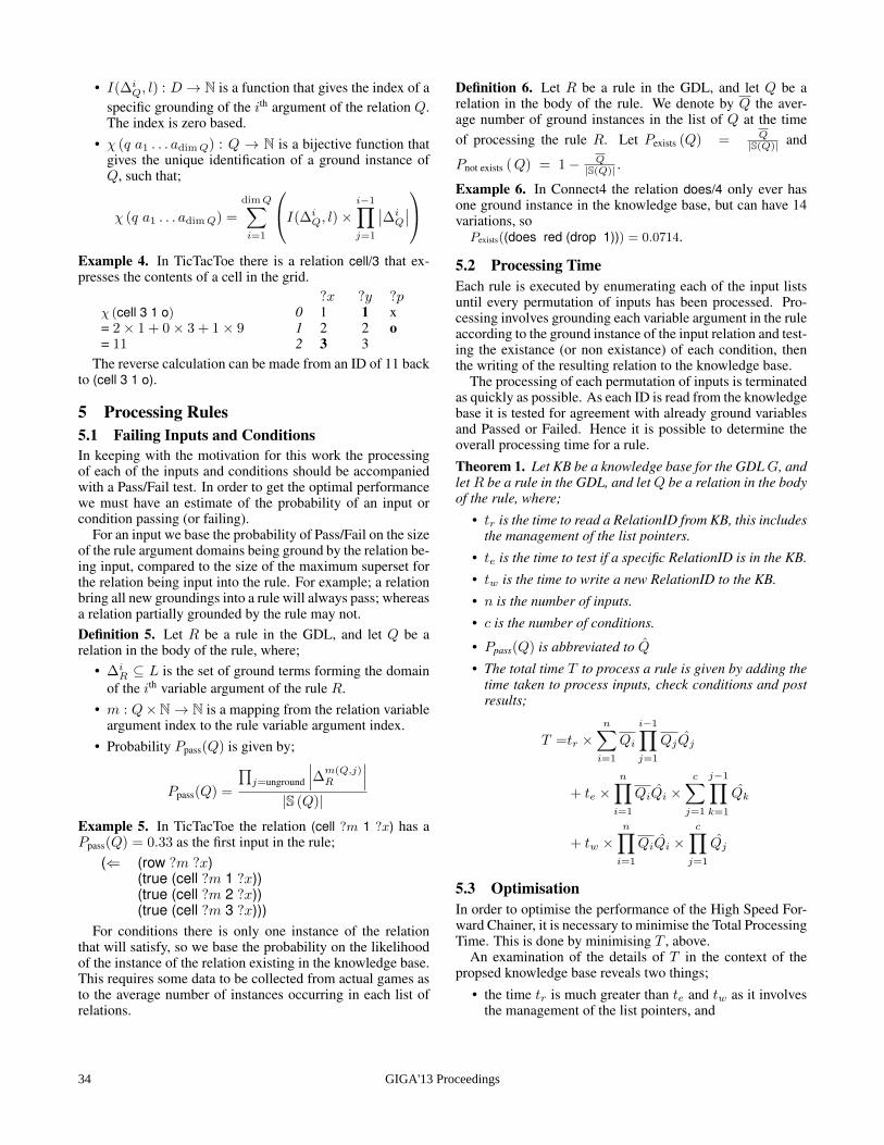
• I(∆iQ, l) : D → N is a function that gives the index of a
specific grounding of the ith argument of the relation Q.The index is zero based.
• χ (q a1 . . . adimQ) : Q → N is a bijective function thatgives the unique identification of a ground instance ofQ, such that;
χ (q a1 . . . adimQ) =
dimQ∑i=1
I(∆iQ, l)×
i−1∏j=1
∣∣∆iQ
∣∣Example 4. In TicTacToe there is a relation cell/3 that ex-presses the contents of a cell in the grid.
?x ?y ?pχ (cell 3 1 o) 0 1 1 x= 2× 1 + 0× 3 + 1× 9 1 2 2 o= 11 2 3 3
The reverse calculation can be made from an ID of 11 backto (cell 3 1 o).
5 Processing Rules5.1 Failing Inputs and ConditionsIn keeping with the motivation for this work the processingof each of the inputs and conditions should be accompaniedwith a Pass/Fail test. In order to get the optimal performancewe must have an estimate of the probability of an input orcondition passing (or failing).
For an input we base the probability of Pass/Fail on the sizeof the rule argument domains being ground by the relation be-ing input, compared to the size of the maximum superset forthe relation being input into the rule. For example; a relationbring all new groundings into a rule will always pass; whereasa relation partially grounded by the rule may not.Definition 5. Let R be a rule in the GDL, and let Q be arelation in the body of the rule, where;
• ∆iR ⊆ L is the set of ground terms forming the domain
of the ith variable argument of the rule R.• m : Q×N→ N is a mapping from the relation variable
argument index to the rule variable argument index.• Probability Ppass(Q) is given by;
Ppass(Q) =
∏j=unground
∣∣∣∆m(Q,j)R
∣∣∣|S (Q)|
Example 5. In TicTacToe the relation (cell ?m 1 ?x) has aPpass(Q) = 0.33 as the first input in the rule;
(⇐ (row ?m ?x)(true (cell ?m 1 ?x))(true (cell ?m 2 ?x))(true (cell ?m 3 ?x)))
For conditions there is only one instance of the relationthat will satisfy, so we base the probability on the likelihoodof the instance of the relation existing in the knowledge base.This requires some data to be collected from actual games asto the average number of instances occurring in each list ofrelations.
Definition 6. Let R be a rule in the GDL, and let Q be arelation in the body of the rule. We denote by Q the aver-age number of ground instances in the list of Q at the timeof processing the rule R. Let Pexists (Q) = Q
|S(Q)| and
Pnot exists (Q) = 1− Q|S(Q)| .
Example 6. In Connect4 the relation does/4 only ever hasone ground instance in the knowledge base, but can have 14variations, soPexists((does red (drop 1))) = 0.0714.
5.2 Processing TimeEach rule is executed by enumerating each of the input listsuntil every permutation of inputs has been processed. Pro-cessing involves grounding each variable argument in the ruleaccording to the ground instance of the input relation and test-ing the existance (or non existance) of each condition, thenthe writing of the resulting relation to the knowledge base.
The processing of each permutation of inputs is terminatedas quickly as possible. As each ID is read from the knowledgebase it is tested for agreement with already ground variablesand Passed or Failed. Hence it is possible to determine theoverall processing time for a rule.
Theorem 1. Let KB be a knowledge base for the GDLG, andletR be a rule in the GDL, and letQ be a relation in the bodyof the rule, where;
• tr is the time to read a RelationID from KB, this includesthe management of the list pointers.
• te is the time to test if a specific RelationID is in the KB.
• tw is the time to write a new RelationID to the KB.
• n is the number of inputs.
• c is the number of conditions.
• Ppass(Q) is abbreviated to Q
• The total time T to process a rule is given by adding thetime taken to process inputs, check conditions and postresults;
T =tr ×n∑
i=1
Qi
i−1∏j=1
QjQj
+ te ×n∏
i=1
QiQi ×c∑
j=1
j−1∏k=1
Qk
+ tw ×n∏
i=1
QiQi ×c∏
j=1
Qj
5.3 OptimisationIn order to optimise the performance of the High Speed For-ward Chainer, it is necessary to minimise the Total ProcessingTime. This is done by minimising T , above.
An examination of the details of T in the context of thepropsed knowledge base reveals two things;
• the time tr is much greater than te and tw as it involvesthe management of the list pointers, and
GIGA'13 Proceedings34
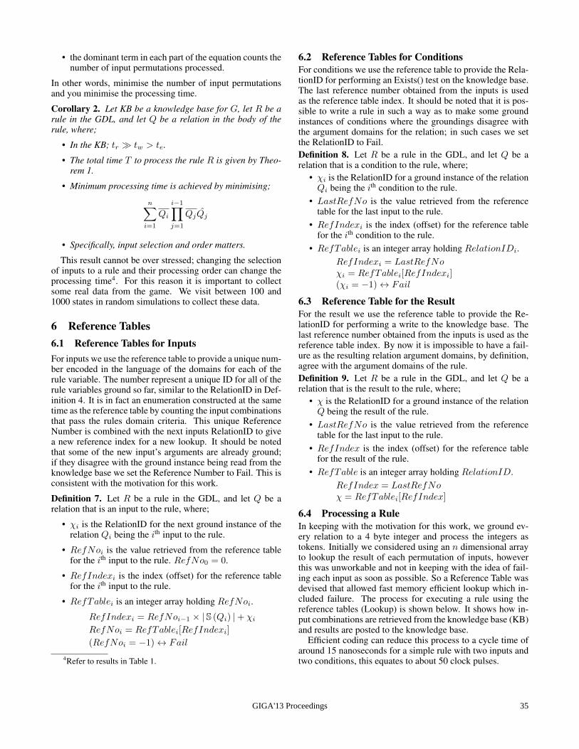
• the dominant term in each part of the equation counts thenumber of input permutations processed.
In other words, minimise the number of input permutationsand you minimise the processing time.
Corollary 2. Let KB be a knowledge base for G, let R be arule in the GDL, and let Q be a relation in the body of therule, where;
• In the KB; tr tw > te.
• The total time T to process the rule R is given by Theo-rem 1.
• Minimum processing time is achieved by minimising;
n∑i=1
Qi
i−1∏j=1
QjQj
• Specifically, input selection and order matters.
This result cannot be over stressed; changing the selectionof inputs to a rule and their processing order can change theprocessing time4. For this reason it is important to collectsome real data from the game. We visit between 100 and1000 states in random simulations to collect these data.
6 Reference Tables6.1 Reference Tables for InputsFor inputs we use the reference table to provide a unique num-ber encoded in the language of the domains for each of therule variable. The number represent a unique ID for all of therule variables ground so far, similar to the RelationID in Def-inition 4. It is in fact an enumeration constructed at the sametime as the reference table by counting the input combinationsthat pass the rules domain criteria. This unique ReferenceNumber is combined with the next inputs RelationID to givea new reference index for a new lookup. It should be notedthat some of the new input’s arguments are already ground;if they disagree with the ground instance being read from theknowledge base we set the Reference Number to Fail. This isconsistent with the motivation for this work.
Definition 7. Let R be a rule in the GDL, and let Q be arelation that is an input to the rule, where;
• χi is the RelationID for the next ground instance of therelation Qi being the ith input to the rule.
• RefNoi is the value retrieved from the reference tablefor the ith input to the rule. RefNo0 = 0.
• RefIndexi is the index (offset) for the reference tablefor the ith input to the rule.
• RefTablei is an integer array holding RefNoi.
RefIndexi = RefNoi−1 × | S (Qi) |+ χi
RefNoi = RefTablei[RefIndexi]
(RefNoi = −1)↔ Fail
4Refer to results in Table 1.
6.2 Reference Tables for ConditionsFor conditions we use the reference table to provide the Rela-tionID for performing an Exists() test on the knowledge base.The last reference number obtained from the inputs is usedas the reference table index. It should be noted that it is pos-sible to write a rule in such a way as to make some groundinstances of conditions where the groundings disagree withthe argument domains for the relation; in such cases we setthe RelationID to Fail.Definition 8. Let R be a rule in the GDL, and let Q be arelation that is a condition to the rule, where;
• χi is the RelationID for a ground instance of the relationQi being the ith condition to the rule.
• LastRefNo is the value retrieved from the referencetable for the last input to the rule.
• RefIndexi is the index (offset) for the reference tablefor the ith condition to the rule.
• RefTablei is an integer array holding RelationIDi.RefIndexi = LastRefNoχi = RefTablei[RefIndexi](χi = −1)↔ Fail
6.3 Reference Table for the ResultFor the result we use the reference table to provide the Re-lationID for performing a write to the knowledge base. Thelast reference number obtained from the inputs is used as thereference table index. By now it is impossible to have a fail-ure as the resulting relation argument domains, by definition,agree with the argument domains of the rule.Definition 9. Let R be a rule in the GDL, and let Q be arelation that is the result to the rule, where;
• χ is the RelationID for a ground instance of the relationQ being the result of the rule.
• LastRefNo is the value retrieved from the referencetable for the last input to the rule.
• RefIndex is the index (offset) for the reference tablefor the result of the rule.
• RefTable is an integer array holding RelationID.RefIndex = LastRefNoχ = RefTablei[RefIndex]
6.4 Processing a RuleIn keeping with the motivation for this work, we ground ev-ery relation to a 4 byte integer and process the integers astokens. Initially we considered using an n dimensional arrayto lookup the result of each permutation of inputs, howeverthis was unworkable and not in keeping with the idea of fail-ing each input as soon as possible. So a Reference Table wasdevised that allowed fast memory efficient lookup which in-cluded failure. The process for executing a rule using thereference tables (Lookup) is shown below. It shows how in-put combinations are retrieved from the knowledge base (KB)and results are posted to the knowledge base.
Efficient coding can reduce this process to a cycle time ofaround 15 nanoseconds for a simple rule with two inputs andtwo conditions, this equates to about 50 clock pulses.
GIGA'13 Proceedings 35
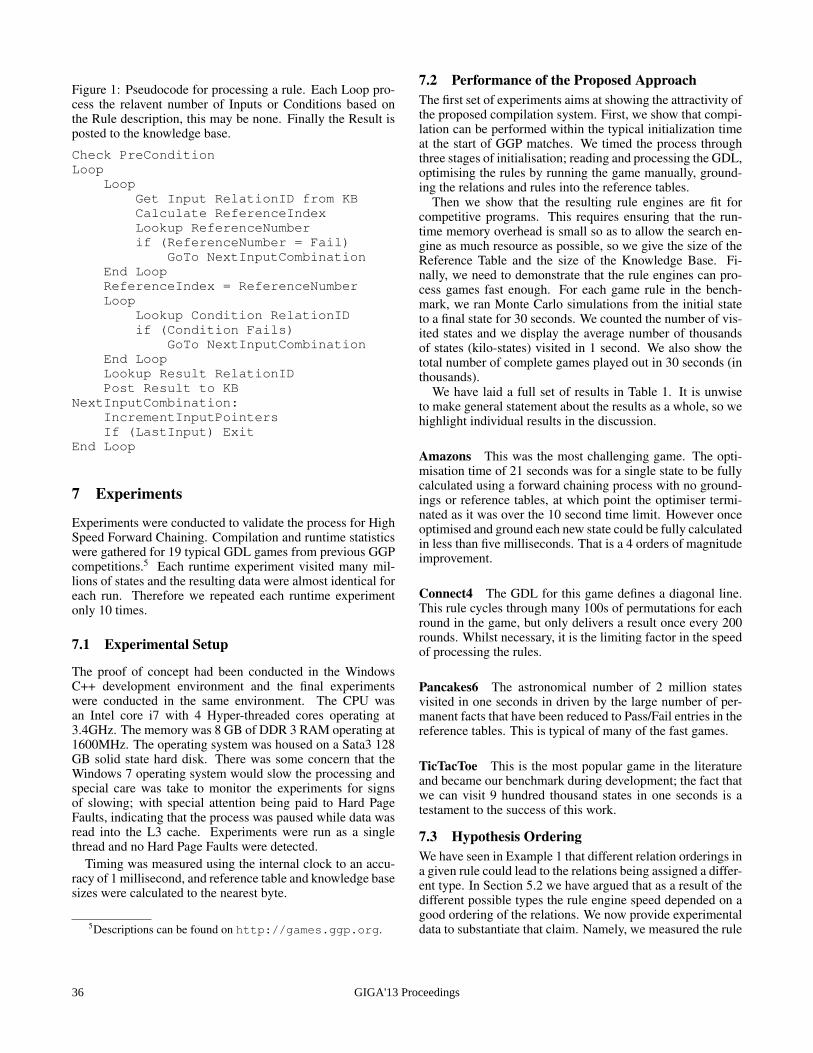
Figure 1: Pseudocode for processing a rule. Each Loop pro-cess the relavent number of Inputs or Conditions based onthe Rule description, this may be none. Finally the Result isposted to the knowledge base.
Check PreConditionLoop
LoopGet Input RelationID from KBCalculate ReferenceIndexLookup ReferenceNumberif (ReferenceNumber = Fail)
GoTo NextInputCombinationEnd LoopReferenceIndex = ReferenceNumberLoop
Lookup Condition RelationIDif (Condition Fails)
GoTo NextInputCombinationEnd LoopLookup Result RelationIDPost Result to KB
NextInputCombination:IncrementInputPointersIf (LastInput) Exit
End Loop
7 Experiments
Experiments were conducted to validate the process for HighSpeed Forward Chaining. Compilation and runtime statisticswere gathered for 19 typical GDL games from previous GGPcompetitions.5 Each runtime experiment visited many mil-lions of states and the resulting data were almost identical foreach run. Therefore we repeated each runtime experimentonly 10 times.
7.1 Experimental Setup
The proof of concept had been conducted in the WindowsC++ development environment and the final experimentswere conducted in the same environment. The CPU wasan Intel core i7 with 4 Hyper-threaded cores operating at3.4GHz. The memory was 8 GB of DDR 3 RAM operating at1600MHz. The operating system was housed on a Sata3 128GB solid state hard disk. There was some concern that theWindows 7 operating system would slow the processing andspecial care was take to monitor the experiments for signsof slowing; with special attention being paid to Hard PageFaults, indicating that the process was paused while data wasread into the L3 cache. Experiments were run as a singlethread and no Hard Page Faults were detected.
Timing was measured using the internal clock to an accu-racy of 1 millisecond, and reference table and knowledge basesizes were calculated to the nearest byte.
5Descriptions can be found on http://games.ggp.org.
7.2 Performance of the Proposed ApproachThe first set of experiments aims at showing the attractivity ofthe proposed compilation system. First, we show that compi-lation can be performed within the typical initialization timeat the start of GGP matches. We timed the process throughthree stages of initialisation; reading and processing the GDL,optimising the rules by running the game manually, ground-ing the relations and rules into the reference tables.
Then we show that the resulting rule engines are fit forcompetitive programs. This requires ensuring that the run-time memory overhead is small so as to allow the search en-gine as much resource as possible, so we give the size of theReference Table and the size of the Knowledge Base. Fi-nally, we need to demonstrate that the rule engines can pro-cess games fast enough. For each game rule in the bench-mark, we ran Monte Carlo simulations from the initial stateto a final state for 30 seconds. We counted the number of vis-ited states and we display the average number of thousandsof states (kilo-states) visited in 1 second. We also show thetotal number of complete games played out in 30 seconds (inthousands).
We have laid a full set of results in Table 1. It is unwiseto make general statement about the results as a whole, so wehighlight individual results in the discussion.
Amazons This was the most challenging game. The opti-misation time of 21 seconds was for a single state to be fullycalculated using a forward chaining process with no ground-ings or reference tables, at which point the optimiser termi-nated as it was over the 10 second time limit. However onceoptimised and ground each new state could be fully calculatedin less than five milliseconds. That is a 4 orders of magnitudeimprovement.
Connect4 The GDL for this game defines a diagonal line.This rule cycles through many 100s of permutations for eachround in the game, but only delivers a result once every 200rounds. Whilst necessary, it is the limiting factor in the speedof processing the rules.
Pancakes6 The astronomical number of 2 million statesvisited in one seconds in driven by the large number of per-manent facts that have been reduced to Pass/Fail entries in thereference tables. This is typical of many of the fast games.
TicTacToe This is the most popular game in the literatureand became our benchmark during development; the fact thatwe can visit 9 hundred thousand states in one seconds is atestament to the success of this work.
7.3 Hypothesis OrderingWe have seen in Example 1 that different relation orderings ina given rule could lead to the relations being assigned a differ-ent type. In Section 5.2 we have argued that as a result of thedifferent possible types the rule engine speed depended on agood ordering of the relations. We now provide experimentaldata to substantiate that claim. Namely, we measured the rule
GIGA'13 Proceedings36
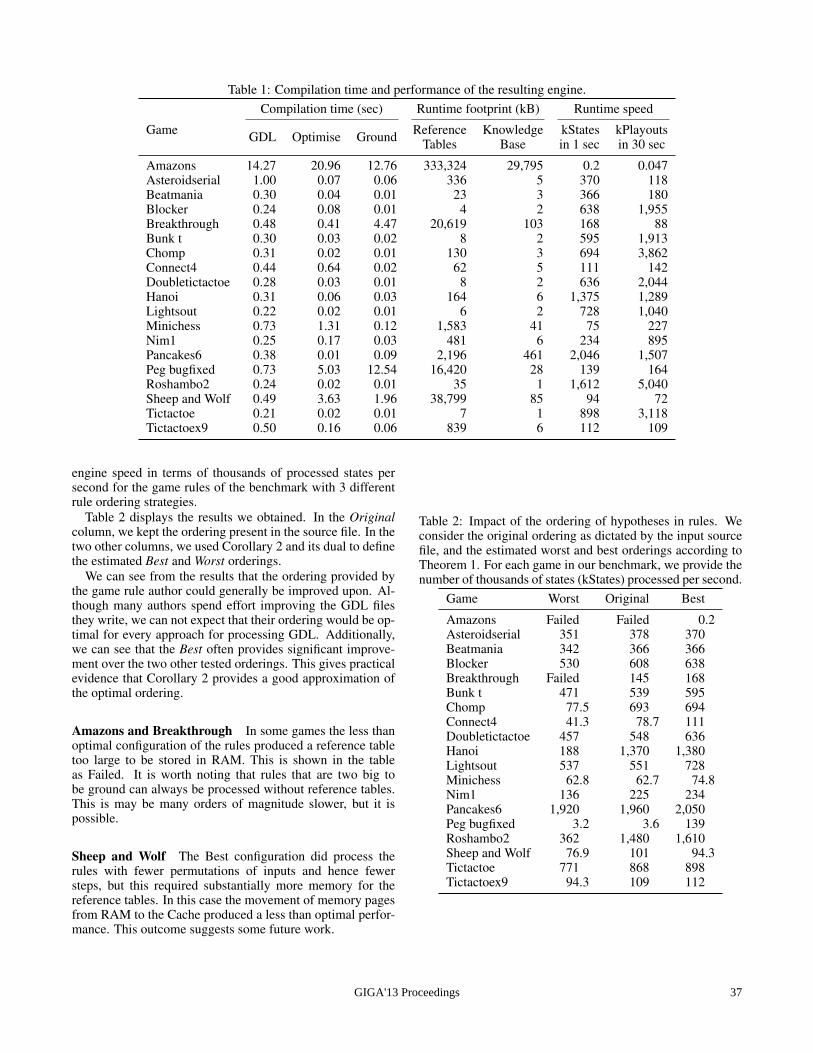
Table 1: Compilation time and performance of the resulting engine.Compilation time (sec) Runtime footprint (kB) Runtime speed
Game GDL Optimise Ground Reference Knowledge kStates kPlayoutsTables Base in 1 sec in 30 sec
Amazons 14.27 20.96 12.76 333,324 29,795 0.2 0.047Asteroidserial 1.00 0.07 0.06 336 5 370 118Beatmania 0.30 0.04 0.01 23 3 366 180Blocker 0.24 0.08 0.01 4 2 638 1,955Breakthrough 0.48 0.41 4.47 20,619 103 168 88Bunk t 0.30 0.03 0.02 8 2 595 1,913Chomp 0.31 0.02 0.01 130 3 694 3,862Connect4 0.44 0.64 0.02 62 5 111 142Doubletictactoe 0.28 0.03 0.01 8 2 636 2,044Hanoi 0.31 0.06 0.03 164 6 1,375 1,289Lightsout 0.22 0.02 0.01 6 2 728 1,040Minichess 0.73 1.31 0.12 1,583 41 75 227Nim1 0.25 0.17 0.03 481 6 234 895Pancakes6 0.38 0.01 0.09 2,196 461 2,046 1,507Peg bugfixed 0.73 5.03 12.54 16,420 28 139 164Roshambo2 0.24 0.02 0.01 35 1 1,612 5,040Sheep and Wolf 0.49 3.63 1.96 38,799 85 94 72Tictactoe 0.21 0.02 0.01 7 1 898 3,118Tictactoex9 0.50 0.16 0.06 839 6 112 109
engine speed in terms of thousands of processed states persecond for the game rules of the benchmark with 3 differentrule ordering strategies.
Table 2 displays the results we obtained. In the Originalcolumn, we kept the ordering present in the source file. In thetwo other columns, we used Corollary 2 and its dual to definethe estimated Best and Worst orderings.
We can see from the results that the ordering provided bythe game rule author could generally be improved upon. Al-though many authors spend effort improving the GDL filesthey write, we can not expect that their ordering would be op-timal for every approach for processing GDL. Additionally,we can see that the Best often provides significant improve-ment over the two other tested orderings. This gives practicalevidence that Corollary 2 provides a good approximation ofthe optimal ordering.
Amazons and Breakthrough In some games the less thanoptimal configuration of the rules produced a reference tabletoo large to be stored in RAM. This is shown in the tableas Failed. It is worth noting that rules that are two big tobe ground can always be processed without reference tables.This is may be many orders of magnitude slower, but it ispossible.
Sheep and Wolf The Best configuration did process therules with fewer permutations of inputs and hence fewersteps, but this required substantially more memory for thereference tables. In this case the movement of memory pagesfrom RAM to the Cache produced a less than optimal perfor-mance. This outcome suggests some future work.
Table 2: Impact of the ordering of hypotheses in rules. Weconsider the original ordering as dictated by the input sourcefile, and the estimated worst and best orderings according toTheorem 1. For each game in our benchmark, we provide thenumber of thousands of states (kStates) processed per second.
Game Worst Original Best
Amazons Failed Failed 0.2Asteroidserial 351 378 370Beatmania 342 366 366Blocker 530 608 638Breakthrough Failed 145 168Bunk t 471 539 595Chomp 77.5 693 694Connect4 41.3 78.7 111Doubletictactoe 457 548 636Hanoi 188 1,370 1,380Lightsout 537 551 728Minichess 62.8 62.7 74.8Nim1 136 225 234Pancakes6 1,920 1,960 2,050Peg bugfixed 3.2 3.6 139Roshambo2 362 1,480 1,610Sheep and Wolf 76.9 101 94.3Tictactoe 771 868 898Tictactoex9 94.3 109 112
GIGA'13 Proceedings 37
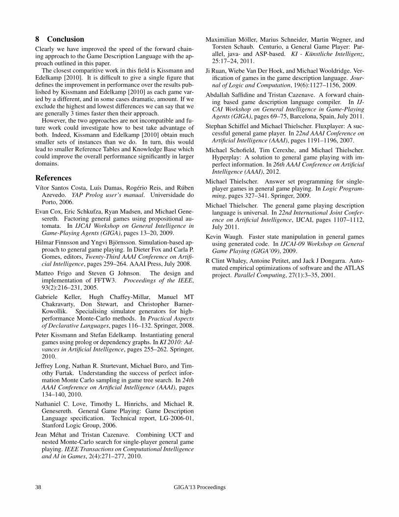
8 ConclusionClearly we have improved the speed of the forward chain-ing approach to the Game Description Language with the ap-proach outlined in this paper.
The closest comparitive work in this field is Kissmann andEdelkamp [2010]. It is difficult to give a single figure thatdefines the improvement in performance over the results pub-lished by Kissmann and Edelkamp [2010] as each game var-ied by a different, and in some cases dramatic, amount. If weexclude the highest and lowest differences we can say that weare generally 3 times faster then their approach.
However, the two approaches are not incompatible and fu-ture work could investigate how to best take advantage ofboth. Indeed, Kissmann and Edelkamp [2010] obtain muchsmaller sets of instances than we do. In turn, this wouldlead to smaller Reference Tables and Knowledge Base whichcould improve the overall performance significantly in largerdomains.
ReferencesVıtor Santos Costa, Luıs Damas, Rogerio Reis, and Ruben
Azevedo. YAP Prolog user’s manual. Universidade doPorto, 2006.
Evan Cox, Eric Schkufza, Ryan Madsen, and Michael Gene-sereth. Factoring general games using propositional au-tomata. In IJCAI Workshop on General Intelligence inGame-Playing Agents (GIGA), pages 13–20, 2009.
Hilmar Finnsson and Yngvi Bjornsson. Simulation-based ap-proach to general game playing. In Dieter Fox and Carla P.Gomes, editors, Twenty-Third AAAI Conference on Artifi-cial Intelligence, pages 259–264. AAAI Press, July 2008.
Matteo Frigo and Steven G Johnson. The design andimplementation of FFTW3. Proceedings of the IEEE,93(2):216–231, 2005.
Gabriele Keller, Hugh Chaffey-Millar, Manuel MTChakravarty, Don Stewart, and Christopher Barner-Kowollik. Specialising simulator generators for high-performance Monte-Carlo methods. In Practical Aspectsof Declarative Languages, pages 116–132. Springer, 2008.
Peter Kissmann and Stefan Edelkamp. Instantiating generalgames using prolog or dependency graphs. In KI 2010: Ad-vances in Artificial Intelligence, pages 255–262. Springer,2010.
Jeffrey Long, Nathan R. Sturtevant, Michael Buro, and Tim-othy Furtak. Understanding the success of perfect infor-mation Monte Carlo sampling in game tree search. In 24thAAAI Conference on Artificial Intelligence (AAAI), pages134–140, 2010.
Nathaniel C. Love, Timothy L. Hinrichs, and Michael R.Genesereth. General Game Playing: Game DescriptionLanguage specification. Technical report, LG-2006-01,Stanford Logic Group, 2006.
Jean Mehat and Tristan Cazenave. Combining UCT andnested Monte-Carlo search for single-player general gameplaying. IEEE Transactions on Computational Intelligenceand AI in Games, 2(4):271–277, 2010.
Maximilian Moller, Marius Schneider, Martin Wegner, andTorsten Schaub. Centurio, a General Game Player: Par-allel, java- and ASP-based. KI - Kunstliche Intelligenz,25:17–24, 2011.
Ji Ruan, Wiebe Van Der Hoek, and Michael Wooldridge. Ver-ification of games in the game description language. Jour-nal of Logic and Computation, 19(6):1127–1156, 2009.
Abdallah Saffidine and Tristan Cazenave. A forward chain-ing based game description language compiler. In IJ-CAI Workshop on General Intelligence in Game-PlayingAgents (GIGA), pages 69–75, Barcelona, Spain, July 2011.
Stephan Schiffel and Michael Thielscher. Fluxplayer: A suc-cessful general game player. In 22nd AAAI Conference onArtificial Intelligence (AAAI), pages 1191–1196, 2007.
Michael Schofield, Tim Cerexhe, and Michael Thielscher.Hyperplay: A solution to general game playing with im-perfect information. In 26th AAAI Conference on ArtificialIntelligence (AAAI), 2012.
Michael Thielscher. Answer set programming for single-player games in general game playing. In Logic Program-ming, pages 327–341. Springer, 2009.
Michael Thielscher. The general game playing descriptionlanguage is universal. In 22nd International Joint Confer-ence on Artificial Intelligence, IJCAI, pages 1107–1112,July 2011.
Kevin Waugh. Faster state manipulation in general gamesusing generated code. In IJCAI-09 Workshop on GeneralGame Playing (GIGA’09), 2009.
R Clint Whaley, Antoine Petitet, and Jack J Dongarra. Auto-mated empirical optimizations of software and the ATLASproject. Parallel Computing, 27(1):3–35, 2001.
GIGA'13 Proceedings38
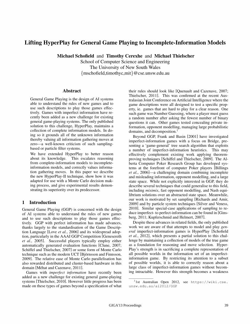
Lifting HyperPlay for General Game Playing to Incomplete-Information Models
Michael Schofield and Timothy Cerexhe and Michael ThielscherSchool of Computer Science and Engineering
The University of New South Walesmschofield,timothyc,[email protected]
AbstractGeneral Game Playing is the design of AI systemsable to understand the rules of new games and touse such descriptions to play those games effec-tively. Games with imperfect information have re-cently been added as a new challenge for existinggeneral game-playing systems. The only publishedsolution to this challenge, HyperPlay, maintains acollection of complete information models. In do-ing so it grounds all of the unknown informationthereby valuing all information gathering moves atzero—a well-known criticism of such sampling-based or particle filter systems.We have extended HyperPlay to better reasonabout its knowledge. This escalates reasoningfrom complete-information models to incomplete-information models, and correctly values informa-tion gathering moves. In this paper we describethe new HyperPlay-II technique, show how it wasadapted for use with a Monte Carlo decision mak-ing process, and give experimental results demon-strating its superiority over its predecessor.
1 IntroductionGeneral Game Playing (GGP) is concerned with the designof AI systems able to understand the rules of new gamesand to use such descriptions to play those games effec-tively. GGP with perfect information has made advances,thanks largely to the standardisation of the Game Descrip-tion Language [Love et al., 2006] and its widespread adop-tion, particularly in the AAAI GGP Competition [Geneserethet al., 2005]. Successful players typically employ eitherautomatically generated evaluation functions [Clune, 2007;Schiffel and Thielscher, 2007] or some form of Monte Carlotechnique such as the modern UCT [Bjornsson and Finnsson,2009]. The relative ease of Monte Carlo parallelisation hasalso rewarded distributed and cluster-based hardware in thisdomain [Mehat and Cazenave, 2011].
Games with imperfect information have recently beenadded as a new challenge for existing general game-playingsystems [Thielscher, 2010]. However little progress has beenmade on these types of games beyond a specification of what
their rules should look like [Quenault and Cazenave, 2007;Thielscher, 2011]. This was confirmed at the recent Aus-tralasian Joint Conference on Artificial Intelligence where thegame descriptions were all designed to test a specific prop-erty, ie. games that are hard to play for a clear reason. Onesuch game was Number Guessing, where a player must guessa random number after asking the fewest number of binaryquestions it can. Other games tested concealing private in-formation, opponent modelling, managing large probabilisticdomains, and decomposition.1
Beyond GGP, Frank and Basin [2001] have investigatedimperfect-information games with a focus on Bridge, pre-senting a ‘game-general’ tree search algorithm that exploitsa number of imperfect-information heuristics. This mayeffectively complement existing work applying theorem-proving techniques [Schiffel and Thielscher, 2009]. The Al-berta Computer Poker Research Group has developed sys-tems at the forefront of computer Poker players [Billingset al., 2006]—a challenging domain combining incompleteand misleading information, opponent modelling, and a largestate space. While not explicitly interested in GGP, they dodescribe several techniques that could generalise to this field,including miximix, fast opponent modelling, and Nash equi-librium solutions over an abstracted state space. Meanwhile,our work is motivated by set sampling [Richards and Amir,2009] and by particle system techniques [Silver and Veness,2010]. Similar special-case applications of sampling to re-duce imperfect- to perfect-information can be found in [Gins-berg, 2011; Kupferschmid and Helmert, 2007].
Despite these advances in related fields, the only publishedwork we are aware of that attempts to model and play gen-eral imperfect-information games is HyperPlay [Schofieldet al., 2012], which presents a partial solution to this chal-lenge by maintaining a collection of models of the true gameas a foundation for reasoning and move selection. Hyper-Play’s strength is in sacrificing a complete representation ofall possible worlds in the information set of an imperfect-information game. By restricting its attention to a subsetof possible worlds, it is able to correctly reason about alarge class of imperfect-information games without becom-ing intractable. However this strength becomes a weakness
11st Australian Open 2012, see https://wiki.cse.unsw.edu.au/ai2012/GGP
GIGA'13 Proceedings 39
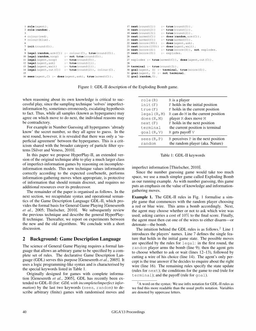
1 role(agent).2 role(random).34 colour(red).5 colour(blue).67 init(round(0)).89 legal(random,arm(C)) :- colour(C), true(round(0)).
10 legal(random,noop) :- not true(round(0)).11 legal(agent,noop) :- true(round(0)).12 legal(agent,ask) :- true(round(1)).13 legal(agent,wait) :- true(round(1)).14 legal(agent,cut(C)) :- true(round(2)), colour(C).1516 sees(agent,C) :- does(agent,ask), true(armed(C)).
17 next(round(1)) :- true(round(0)).18 next(round(2)) :- true(round(1)).19 next(round(3)) :- true(round(2)).20 next(armed(C)) :- does(random,arm(C)).21 next(armed(C)) :- true(armed(C)).22 next(score(90)) :- does(agent,ask).23 next(score(100)) :- does(agent,wait).24 next(score(S)) :- true(score(S)), not explodes.25 next(score(0)) :- explodes.2627 explodes :- true(armed(C)), does(agent,cut(C)).2829 terminal :- true(round(3)).30 goal(agent, S) :- terminal, true(score(S)).31 goal(agent, 0) :- not terminal.32 goal(random,0).
Figure 1: GDL-II description of the Exploding Bomb game.
when reasoning about its own knowledge is critical to suc-cessful play, since the sampling technique ‘solves’ imperfect-information by, sometimes erroneously, escalating hypothesisto fact. Thus, while all samples (known as hypergames) mayagree on which move to do next, the individual reasons maybe contradictory.
For example in Number Guessing all hypergames ‘alreadyknow’ the secret number, so they all agree to guess. In thenext round, however, it is revealed that there was only a ‘su-perficial agreement’ between the hypergames. This is a crit-icism shared with the broader category of particle filter sys-tems [Silver and Veness, 2010].
In this paper we propose HyperPlay-II, an extended ver-sion of the original technique able to play a much larger classof imperfect-information games by reasoning on incomplete-information models. This new technique values informationcorrectly according to the expected cost/benefit, performsinformation-gathering moves when appropriate, is protectiveof information that should remain discreet, and requires noadditional resources over its predecessor.
The remainder of the paper is organised as follows. In thenext section, we recapitulate syntax and operational seman-tics of the Game Description Language GDL-II, which pro-vides the formal basis for General Game Playing [Geneserethet al., 2005; Thielscher, 2010]. We subsequently reviewthe previous technique and describe the general HyperPlay-II technique. Thereafter, we report on experiments betweenthe new and the old algorithms. We conclude with a shortdiscussion.
2 Background: Game Description LanguageThe science of General Game Playing requires a formal lan-guage that allows an arbitrary game to be specified by a com-plete set of rules. The declarative Game Description Lan-guage (GDL) serves this purpose [Genesereth et al., 2005]. Ituses a logic programming-like syntax and is characterised bythe special keywords listed in Table 1.
Originally designed for games with complete informa-tion [Genesereth et al., 2005], GDL has recently been ex-tended to GDL-II (for: GDL with incomplete/imperfect infor-mation) by the last two keywords (sees, random) to de-scribe arbitrary (finite) games with randomised moves and
role(R) R is a playerinit(F) F holds in the initial positiontrue(F) F holds in the current positionlegal(R,M) R can do M in the current positiondoes(R,M) player R does move Mnext(F) F holds in the next positionterminal the current position is terminalgoal(R,V) R gets payoff V
sees(R,P) R perceives P in the next positionrandom the random player (aka. Nature)
Table 1: GDL-II keywords
imperfect information [Thielscher, 2010].Since the number guessing game would take too much
space, we use a much simpler game called Exploding Bombas our running example. As with number guessing, this gameputs an emphasis on the value of knowledge and information-gathering moves.
Example 1. The GDL-II rules in Fig. 1 formalise a sim-ple game that commences with the random player choosinga red or blue wire. This arms a bomb accordingly. Next,the agent may choose whether or not to ask which wire wasused; asking carries a cost of 10% to the final score. Finally,the agent must then cut one of the wires to either disarm—ordetonate—the bomb.
The intuition behind the GDL rules is as follows.2 Line 1introduces the players’ names. Line 7 defines the single fea-ture that holds in the initial game state. The possible movesare specified by the rules for legal: in the first round, therandom player arms the bomb (line 9); then the agent getsto choose whether to ask or wait (lines 12–13), followed bycutting a wire of his choice (line 14). The agent’s only per-cept is the true answer if he decides to enquire about the rightwire (line 16). The remaining rules specify the state update(rules for next); the conditions for the game to end (rule forterminal); and the payoff (rule for goal).
2A word on the syntax: We use infix notation for GDL-II rules aswe find this more readable than the usual prefix notation. Variablesare denoted by uppercase letters.
GIGA'13 Proceedings40
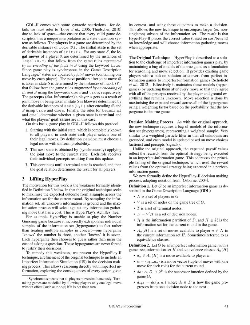
GDL-II comes with some syntactic restrictions—for de-tails we must refer to [Love et al., 2006; Thielscher, 2010]due to lack of space—that ensure that every valid game de-scription has a unique interpretation as a state transition sys-tem as follows. The players in a game are determined by thederivable instances of role(R). The initial state is the setof derivable instances of init(F). For any state S, the le-gal moves of a player R are determined by the instances oflegal(R,M) that follow from the game rules augmentedby an encoding of the facts in S using the keyword true.Since game play is synchronous in the Game DescriptionLanguage,3 states are updated by joint moves (containing onemove by each player). The next position after joint move ~mis taken in state S is determined by the instances of next(F)that follow from the game rules augmented by an encoding of~m and S using the keywords does and true, respectively.The percepts (aka. information) a player R gets as a result ofjoint move ~m being taken in state S is likewise determined bythe derivable instances of sees(R,P) after encoding ~m andS using true and does. Finally, the rules for terminaland goal determine whether a given state is terminal andwhat the players’ goal values are in this case.
On this basis, game play in GDL-II follows this protocol:1. Starting with the initial state, which is completely known
to all players, in each state each player selects one oftheir legal moves. By definition random must choose alegal move with uniform probability.
2. The next state is obtained by (synchronously) applyingthe joint move to the current state. Each role receivestheir individual percepts resulting from this update.
3. This continues until a terminal state is reached, and thenthe goal relation determines the result for all players.
3 Lifting HyperPlayThe motivation for this work is the weakness formally identi-fied in Definition 3 below, in that the original technique seeksto maximise the expected outcome from a sample across theinformation set for the current round. By sampling the infor-mation set, all unknown information is ground and the max-imisation process will select against any information gather-ing move that has a cost. This is HyperPlay’s Achilles’ heel.
For example HyperPlay is unable to play the NumberGuessing game because it incorrectly extrapolates individualsamples of the information set (hypergames) to fact ratherthan treating multiple samples in concert—one hypergame‘knows’ the number is three, another ‘knows’ it is seven.Each hypergame then chooses to guess rather than incur thecost of asking a question. These hypergames are never forcedto justify their decisions.
To remedy this weakness, we present the HyperPlay-IItechnique, a refinement of the original technique to include anImperfect Information Simulation (IIS) in the decision mak-ing process. This allows reasoning directly with imperfect in-formation, exploring the consequences of every action given
3Synchronous means that all players move simultaneously. Turn-taking games are modelled by allowing players only one legal movewithout effect (such as noop) if it is not their turn.
its context, and using these outcomes to make a decision.This allows the new technique to encompass larger (ie. non-singleton) subsets of the information set. The result is thatHyperPlay-II places the correct value (based on cost/benefit)on knowledge and will choose information gathering moveswhen appropriate.
The Original Technique HyperPlay is described as a solu-tion to the challenge of imperfect information games play, bymaintaining a bag of models of the true game as a foundationfor reasoning and move selection. It provides existing gameplayers with a bolt-on solution to convert from perfect in-formation games to imperfect-information games [Schofieldet al., 2012]. Effectively it maintains these models (hyper-games) by updating them after every move so that they agreewith all of the percepts received by the player and ground ev-erything that remains unknown. Move selection is done bymaximising the expected reward across all of the hypergamesusing a weighting factor based on the probability that the hy-pergame is the true game.
Decision Making Process As with the original approach,the new technique requires a bag of models of the informa-tion set (hypergames), representing a weighted sample. Verysimilar to a weighted particle filter in that all unknowns aregrounded, and each model is updated based on move choices(actions) and percepts (signals).
Unlike the original approach, the expected payoff valuesreflect the rewards from the optimal strategy being executedin an imperfect-information game. This addresses the princi-ple failing of the original technique, which used the rewardvalues from the optimal strategy being executed in a perfect-information game.
We now formally define the HyperPlay-II decision makingprocess, adapting notation from [Osborne, 2004].Definition 1. Let G be an imperfect information game as de-scribed in the Game Description Language (GDL)
• N is a set of players in G.• V is a set of nodes on the game tree of G.• T is a set of terminal nodes.• D = V \T is a set of decision nodes.• H is the information partition of D, and H ∈ H is the
information set for the current round in the game.• An(H) is a set of moves available to player n ∈ N in
the current information set H . Sometimes referred to asequivalence classes.
Definition 2. LetG be an imperfect information game, with agame tree, information setH and equivalence classesAn(H)
• an ∈ An(H) is a move available to player n.• α = 〈a1...an〉 is a move vector (tuple of moves with one
move for each role) for the current round.• do : α,D → 2V is the successor function defined by the
game G.• di+1 = do(α, di) where di ∈ D is how the game pro-
gresses from one decision node to the next.
GIGA'13 Proceedings 41
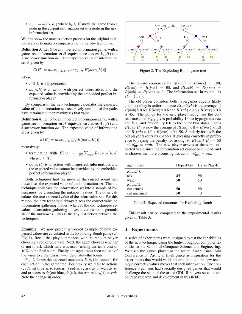
• hi+1 = do(α, hi) where hi ∈ H move the game from anode in the current information set to a node in the nextinformation set.
We first show the move selection process for the original tech-nique so as to make a comparison with the new technique.
Definition 3. LetG be an imperfect information game, with agame tree, information setH , equivalence classesAn(H) anda successor function do. The expected value of informationset is given by
E(H) = maxa∈An(H)[avgh∈H [E(do(a, h))]]
where
• h ∈ H is a hypergame;
• do(a, h) is an action with perfect information, and theexpected value is provided by the embedded perfect in-formation player.
By comparison the new technique calculates the expectedvalue of the information set recursively until all of the pathshave terminated, then maximises that value.
Definition 4. LetG be an imperfect information game, with agame tree, information setH , equivalence classesAn(H) anda successor function do. The expected value of informationset is given by
E(H) = maxa∈An(H)[E(do(a,H))]
recursively,
• terminating with E(τ) = 1|τ |
∑v∈τ Reward(v, n)
where τ ⊆ T ;
• do(a,H) is an action with imperfect information, andthe expected value cannot be provided by the embeddedperfect information player.
Both techniques find the move in the current round thatmaximises the expected value of the information set. The oldtechnique collapses the information set into a sample of hy-pergames, by grounding the unknown values. The other cal-culates the true expected value of the information set. For thisreason, the new technique always places the correct value oninformation gathering moves, whereas the old technique re-values information gathering moves at zero when it groundsall of the unknowns. This is the key distinction between thetechniques.
Example We now present a worked example of how ex-pected values are calculated in the Exploding Bomb game (cf.Fig. 1). Recall that play commences with the random playerchoosing a red or blue wire. Next, the agent chooses whetheror not to ask which wire was used; asking carries a cost of10% to the final score. Finally, the agent must then cut one ofthe wires to either disarm—or detonate—the bomb.
Fig. 2 shows the expected outcomes E(aj) in round 1 foreach action in the game tree. For brevity we refer to actions(cut/arm) blue as b, (cut/arm) red as r, ask as a, wait as w,and to states as do(cut blue, do(ask, do(arm red, v0))) = rab.Note the change in order.
Figure 2: The Exploding Bomb game tree
The reward sequences are R(rwb) = R(bwr) = 100,R(rab) = R(bar) = 90, and R(bwb) = R(rwr) =R(bab) = R(rar) = 0. The information set in round 1 isH = b, r.
The old player considers both hypergames equally likelyand the policy is uniform, hence E(ask|H) is the average ofR(bab)×0.5+R(bar)×0.5 andR(rab)×0.5+R(rar)×0.5is 45. The policy for the new player recognises the cor-rect move, so π∗HPII gives probability 1.0 to hypergames raband bar, and probability 0.0 to the other two states. ThusE(ask|H) is now the average of R(bab)× 0+R(bar)× 1.0and R(rab)×1.0+R(rar)×0 is 90. Similarly for wait, theold player favours its chances at guessing correctly in prefer-ence to paying the penalty for asking, so E(wait H) = 50and a∗HP = wait. The new player arrives at the same ex-pected value since the information set cannot be divided, andso chooses the more promising ask action: a∗HPII = ask.
agent does HyperPlay HyperPlay-II
Round 1:ask 45 90wait 50 50Round 2:cut armed 50 90cut unarmed 50 0
Table 2: Expected outcomes for Exploding Bomb
This result can be compared to the experimental resultsgiven in Table 3.
4 Experiments
A series of experiments were designed to test the capabilitiesof the new technique using the high-throughput computer fa-cilities at the School of Computer Science and Engineering.We used the games played at the recent Australasian JointConference on Artificial Intelligence as inspiration for theexperiments that would validate our claim that the new tech-nique correctly values moves that seek information. The con-ference organisers had specially designed games that wouldchallenge the state of the art of GDL-II players so as to en-courage research and development in this field.
GIGA'13 Proceedings42
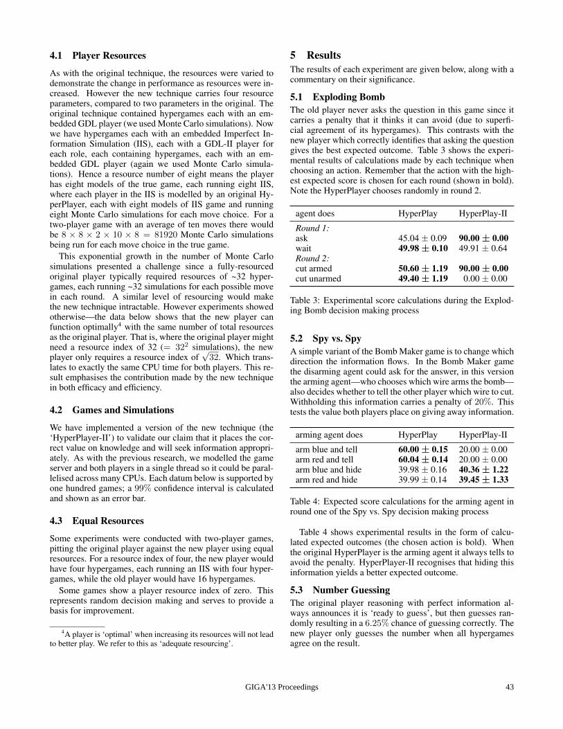
4.1 Player Resources
As with the original technique, the resources were varied todemonstrate the change in performance as resources were in-creased. However the new technique carries four resourceparameters, compared to two parameters in the original. Theoriginal technique contained hypergames each with an em-bedded GDL player (we used Monte Carlo simulations). Nowwe have hypergames each with an embedded Imperfect In-formation Simulation (IIS), each with a GDL-II player foreach role, each containing hypergames, each with an em-bedded GDL player (again we used Monte Carlo simula-tions). Hence a resource number of eight means the playerhas eight models of the true game, each running eight IIS,where each player in the IIS is modelled by an original Hy-perPlayer, each with eight models of IIS game and runningeight Monte Carlo simulations for each move choice. For atwo-player game with an average of ten moves there wouldbe 8 × 8 × 2 × 10 × 8 = 81920 Monte Carlo simulationsbeing run for each move choice in the true game.
This exponential growth in the number of Monte Carlosimulations presented a challenge since a fully-resourcedoriginal player typically required resources of ~32 hyper-games, each running ~32 simulations for each possible movein each round. A similar level of resourcing would makethe new technique intractable. However experiments showedotherwise—the data below shows that the new player canfunction optimally4 with the same number of total resourcesas the original player. That is, where the original player mightneed a resource index of 32 (= 322 simulations), the newplayer only requires a resource index of
√32. Which trans-
lates to exactly the same CPU time for both players. This re-sult emphasises the contribution made by the new techniquein both efficacy and efficiency.
4.2 Games and Simulations
We have implemented a version of the new technique (the‘HyperPlayer-II’) to validate our claim that it places the cor-rect value on knowledge and will seek information appropri-ately. As with the previous research, we modelled the gameserver and both players in a single thread so it could be paral-lelised across many CPUs. Each datum below is supported byone hundred games; a 99% confidence interval is calculatedand shown as an error bar.
4.3 Equal Resources
Some experiments were conducted with two-player games,pitting the original player against the new player using equalresources. For a resource index of four, the new player wouldhave four hypergames, each running an IIS with four hyper-games, while the old player would have 16 hypergames.
Some games show a player resource index of zero. Thisrepresents random decision making and serves to provide abasis for improvement.
4A player is ‘optimal’ when increasing its resources will not leadto better play. We refer to this as ‘adequate resourcing’.
5 ResultsThe results of each experiment are given below, along with acommentary on their significance.
5.1 Exploding BombThe old player never asks the question in this game since itcarries a penalty that it thinks it can avoid (due to superfi-cial agreement of its hypergames). This contrasts with thenew player which correctly identifies that asking the questiongives the best expected outcome. Table 3 shows the experi-mental results of calculations made by each technique whenchoosing an action. Remember that the action with the high-est expected score is chosen for each round (shown in bold).Note the HyperPlayer chooses randomly in round 2.
agent does HyperPlay HyperPlay-II
Round 1:ask 45.04 ± 0.09 90.00 ± 0.00wait 49.98 ± 0.10 49.91 ± 0.64Round 2:cut armed 50.60 ± 1.19 90.00 ± 0.00cut unarmed 49.40 ± 1.19 0.00 ± 0.00
Table 3: Experimental score calculations during the Explod-ing Bomb decision making process
5.2 Spy vs. SpyA simple variant of the Bomb Maker game is to change whichdirection the information flows. In the Bomb Maker gamethe disarming agent could ask for the answer, in this versionthe arming agent—who chooses which wire arms the bomb—also decides whether to tell the other player which wire to cut.Withholding this information carries a penalty of 20%. Thistests the value both players place on giving away information.
arming agent does HyperPlay HyperPlay-II
arm blue and tell 60.00 ± 0.15 20.00 ± 0.00arm red and tell 60.04 ± 0.14 20.00 ± 0.00arm blue and hide 39.98 ± 0.16 40.36 ± 1.22arm red and hide 39.99 ± 0.14 39.45 ± 1.33
Table 4: Expected score calculations for the arming agent inround one of the Spy vs. Spy decision making process
Table 4 shows experimental results in the form of calcu-lated expected outcomes (the chosen action is bold). Whenthe original HyperPlayer is the arming agent it always tells toavoid the penalty. HyperPlayer-II recognises that hiding thisinformation yields a better expected outcome.
5.3 Number GuessingThe original player reasoning with perfect information al-ways announces it is ‘ready to guess’, but then guesses ran-domly resulting in a 6.25% chance of guessing correctly. Thenew player only guesses the number when all hypergamesagree on the result.
GIGA'13 Proceedings 43
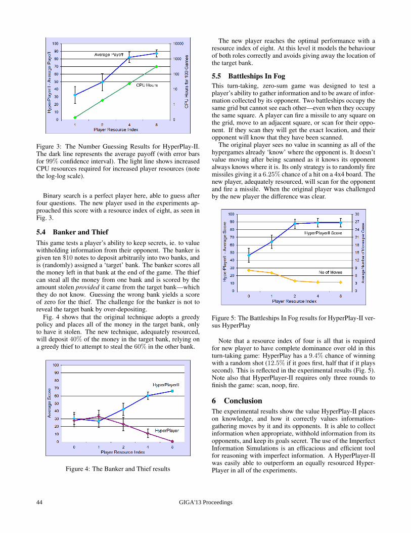
Figure 3: The Number Guessing Results for HyperPlay-II.The dark line represents the average payoff (with error barsfor 99% confidence interval). The light line shows increasedCPU resources required for increased player resources (notethe log-log scale).
Binary search is a perfect player here, able to guess afterfour questions. The new player used in the experiments ap-proached this score with a resource index of eight, as seen inFig. 3.
5.4 Banker and ThiefThis game tests a player’s ability to keep secrets, ie. to valuewithholding information from their opponent. The banker isgiven ten $10 notes to deposit arbitrarily into two banks, andis (randomly) assigned a ‘target’ bank. The banker scores allthe money left in that bank at the end of the game. The thiefcan steal all the money from one bank and is scored by theamount stolen provided it came from the target bank—whichthey do not know. Guessing the wrong bank yields a scoreof zero for the thief. The challenge for the banker is not toreveal the target bank by over-depositing.
Fig. 4 shows that the original technique adopts a greedypolicy and places all of the money in the target bank, onlyto have it stolen. The new technique, adequately resourced,will deposit 40% of the money in the target bank, relying ona greedy thief to attempt to steal the 60% in the other bank.
Figure 4: The Banker and Thief results
The new player reaches the optimal performance with aresource index of eight. At this level it models the behaviourof both roles correctly and avoids giving away the location ofthe target bank.
5.5 Battleships In FogThis turn-taking, zero-sum game was designed to test aplayer’s ability to gather information and to be aware of infor-mation collected by its opponent. Two battleships occupy thesame grid but cannot see each other—even when they occupythe same square. A player can fire a missile to any square onthe grid, move to an adjacent square, or scan for their oppo-nent. If they scan they will get the exact location, and theiropponent will know that they have been scanned.
The original player sees no value in scanning as all of thehypergames already ‘know’ where the opponent is. It doesn’tvalue moving after being scanned as it knows its opponentalways knows where it is. Its only strategy is to randomly firemissiles giving it a 6.25% chance of a hit on a 4x4 board. Thenew player, adequately resourced, will scan for the opponentand fire a missile. When the original player was challengedby the new player the difference was clear.
Figure 5: The Battleships In Fog results for HyperPlay-II ver-sus HyperPlay
Note that a resource index of four is all that is requiredfor new player to have complete dominance over old in thisturn-taking game: HyperPlay has a 9.4% chance of winningwith a random shot (12.5% if it goes first, half that if it playssecond). This is reflected in the experimental results (Fig. 5).Note also that HyperPlayer-II requires only three rounds tofinish the game: scan, noop, fire.
6 ConclusionThe experimental results show the value HyperPlay-II placeson knowledge, and how it correctly values information-gathering moves by it and its opponents. It is able to collectinformation when appropriate, withhold information from itsopponents, and keep its goals secret. The use of the ImperfectInformation Simulations is an efficacious and efficient toolfor reasoning with imperfect information. A HyperPlayer-IIwas easily able to outperform an equally resourced Hyper-Player in all of the experiments.
GIGA'13 Proceedings44

We intend to explore additional features of the HyperPlay-II technique as they pertain to general artificial intelligencethrough the development of the HyperWorlds technique. Thiswill be a more generalised solution, capable of dealing withimperfect information in real-world scenarios.
We also intend to implement the HyperPlayer-II for theGeneral Game Playing arena as a benchmark competitor forother researchers to challenge in GDL-II games.
Acknowledgements. We thank the anonymous review-ers of an earlier version for their constructive com-ments. This research was supported under Australian Re-search Council’s (ARC) Discovery Projects funding scheme(project DP 120102023). Michael Thielscher is the recipientof an ARC Future Fellowship (project FT 0991348). He isalso affiliated with the University of Western Sydney.
References[Billings et al., 2006] Darse Billings, Aaron Davidson, Ter-
ence Schauenberg, Neil Burch, Michael Bowling, RobertHolte, Jonathan Schaeffer, and Duane Szafron. Game-treesearch with adaptation in stochastic imperfect-informationgames. In Proc. Computers and Games, pages 21–34,2006.
[Bjornsson and Finnsson, 2009] Y. Bjornsson and H. Finns-son. CadiaPlayer: A simulation-based general gameplayer. IEEE Transactions on Computational Intelligenceand AI in Games, 1(1):4–15, March 2009.
[Clune, 2007] Jim Clune. Heuristic evaluation functions forgeneral game playing. In Proc. AAAI, pages 1134–1139,Vancouver, July 2007.
[Frank and Basin, 2001] Ian Frank and David Basin. A the-oretical and empirical investigation of search in imperfectinformation games. Theoretical Computer Science, 252(1-2):217–256, 2001.
[Genesereth et al., 2005] Michael R. Genesereth, NathanielLove, and Barney Pell. General game playing: Overviewof the AAAI competition. AI Magazine, 26(2):62–72,2005.
[Ginsberg, 2011] Matthew Ginsberg. GIB: Imperfect infor-mation in a computationally challenging game. CoRR,2011.
[Kupferschmid and Helmert, 2007] Sebastian Kupferschmidand Malte Helmert. A Skat player based on Monte-Carlosimulation. In Proc. Computers and Games, pages 135–147, 2007.
[Love et al., 2006] Nathaniel Love, Timothy Hinrichs,David Haley, Eric Schkufza, and Michael Genesereth.General game playing: Game description languagespecification. Technical Report LG–2006–01, StanfordLogic Group, 2006.
[Mehat and Cazenave, 2011] Jean Mehat and TristanCazenave. A parallel general game player. KI Journal,25(1):43–47, 2011.
[Osborne, 2004] Martin J. Osborne. An introduction to gametheory, volume 3. Oxford University Press, New York, NY,2004.
[Quenault and Cazenave, 2007] M. Quenault andT. Cazenave. Extended general gaming model. InComputer Games Workshop, pages 195–204, 2007.
[Richards and Amir, 2009] Mark Richards and Eyal Amir.Information set sampling for general imperfect informa-tion positional games. In Proc. IJCAI-09 Workshop onGGP (GIGA’09), pages 59–66, 2009.
[Schiffel and Thielscher, 2007] Stephan Schiffel andMichael Thielscher. Fluxplayer: A successful generalgame player. In Proc. AAAI, pages 1191–1196, 2007.
[Schiffel and Thielscher, 2009] Stephan Schiffel andMichael Thielscher. Automated theorem proving forgeneral game playing. In Proc. IJCAI, pages 911–916,2009.
[Schofield et al., 2012] Michael Schofield, TimothyCerexhe, and Michael Thielscher. HyperPlay: Asolution to general game playing with imperfect infor-mation. In Proc. AAAI, pages 1606–1612, Toronto, July2012. AAAI Press.
[Silver and Veness, 2010] David Silver and Joel Veness.Monte-Carlo planning in large POMDPs. In Proc. NIPS,pages 2164–2172, 2010.
[Thielscher, 2010] Michael Thielscher. A general game de-scription language for incomplete information games. InProc. AAAI, pages 994–999, Atlanta, July 2010.
[Thielscher, 2011] Michael Thielscher. The general gameplaying description language is universal. In Proc. IJCAI,pages 1107–1112, Barcelona, July 2011.
GIGA'13 Proceedings 45

GIGA'13 Proceedings46
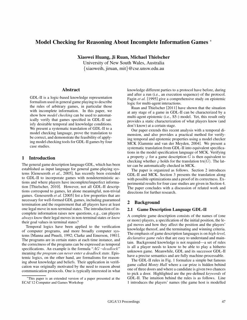
Model Checking for Reasoning About Incomplete Information Games ∗
Xiaowei Huang, Ji Ruan, Michael Thielscher
University of New South Wales, Australia
xiaoweih, jiruan, [email protected]
Abstract
GDL-II is a logic-based knowledge representationformalism used in general game playing to describethe rules of arbitrary games, in particular thosewith incomplete information. In this paper, weshow how model checking can be used to automat-ically verify that games specified in GDL-II sat-isfy desirable temporal and knowledge conditions.We present a systematic translation of GDL-II to amodel checking language, prove the translation tobe correct, and demonstrate the feasibility of apply-ing model checking tools for GDL-II games by fourcase studies.
1 Introduction
The general game description language GDL, which has beenestablished as input language for general game-playing sys-tems [Genesereth et al., 2005], has recently been extendedto GDL-II to incorporate games with nondeterministic ac-tions and where players have incomplete/imperfect informa-tion [Thielscher, 2010]. However, not all GDL-II descrip-tions correspond to games, let alone meaningful, non-trivialgames. Genesereth et al. [2005] list a few properties that arenecessary for well-formed GDL games, including guaranteedtermination and the requirement that all players have at leastone legal move in non-terminal states. The introduction of in-complete information raises new questions, e.g., can playersalways know their legal moves in non-terminal states or knowtheir goal values in terminal states?
Temporal logics have been applied to the verificationof computer programs, and more broadly computer sys-tems [Manna and Pnueli, 1992; Clarke and Emerson, 1981].The programs are in certain states at each time instance, andthe correctness of the programs can be expressed as temporalspecifications. An example is the formula “AG¬deadlock”meaning the program can never enter a deadlock state. Epis-temic logics, on the other hand, are formalisms for reason-ing about knowledge and beliefs. Their application in verifi-cation was originally motivated by the need to reason aboutcommunication protocols. One is typically interested in what
∗This paper is an extended version of a paper presented at theECAI’12 Computer and Games Workshop
knowledge different parties to a protocol have before, duringand after a run (i.e., an execution sequence) of the protocol.Fagin et al. [1995] give a comprehensive study on epistemiclogic for multi-agent interactions.
Ruan and Thielscher [2011] have shown that the situationat any stage of a game in GDL-II can be characterized by amulti-agent epistemic (i.e., S5-) model. Yet, this result onlyprovides a static characterization of what players know (anddon’t know) at a certain stage.
Our paper extends this recent analysis with a temporal di-mension, and also provides a practical method for verify-ing temporal and epistemic properties using a model checkerMCK [Gammie and van der Meyden, 2004]. We present asystematic translation from GDL-II into equivalent specifica-tions in the model specification language of MCK. Verifyinga property ϕ for a game description G is then equivalent tochecking whether ϕ holds for the translation trs(G). The lat-ter can be automatically checked in MCK.
The paper is organized as follows. Section 2 introducesGDL-II and MCK. Section 3 presents the translation alongwith possible optimizations and a proof of its correctness. Ex-perimental results for four case studies are given in Section 4.The paper concludes with a discussion of related work anddirections for further research.
2 Background
2.1 Game Description Language GDL-II
A complete game description consists of the names of (oneor more) players, a specification of the initial position, the le-gal moves and how they affect the position and the players’knowledge thereof, and the terminating and winning criteria.The emphasis of game description languages is on high-level,declarative game rules that are easy to understand and main-tain. Background knowledge is not required—a set of rulesis all a player needs to know to be able to play a hithertounknown game. Meanwhile, GDL and its successor GDL-IIhave a precise semantics and are fully machine-processable.
The GDL-II rules in Fig. 1 formalize a simple but famousgame called Monty Hall where a car prize is hidden behindone of three doors and where a candidate is given two chancesto pick a door. Highlighted are the pre-defined keywords ofGDL-II. The intuition behind the rules is as follows. Line1 introduces the players’ names (the game host is modelled
GIGA'13 Proceedings 47
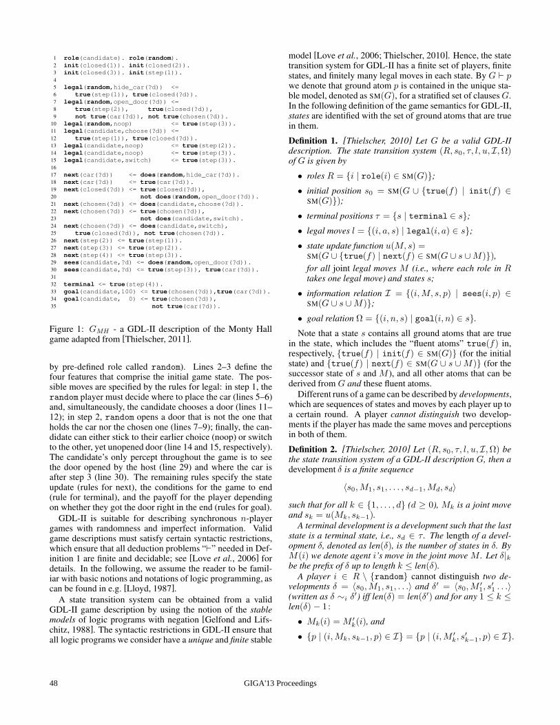
1 role(candidate). role(random).
2 init(closed(1)). init(closed(2)).
3 init(closed(3)). init(step(1)).
4
5 legal(random,hide_car(?d)) <=
6 true(step(1)), true(closed(?d)).
7 legal(random,open_door(?d)) <=
8 true(step(2)), true(closed(?d)),
9 not true(car(?d)), not true(chosen(?d)).
10 legal(random,noop) <= true(step(3)).
11 legal(candidate,choose(?d)) <=
12 true(step(1)), true(closed(?d)).
13 legal(candidate,noop) <= true(step(2)).
14 legal(candidate,noop) <= true(step(3)).
15 legal(candidate,switch) <= true(step(3)).
16
17 next(car(?d)) <= does(random,hide_car(?d)).
18 next(car(?d)) <= true(car(?d)).
19 next(closed(?d)) <= true(closed(?d)),
20 not does(random,open_door(?d)).
21 next(chosen(?d)) <= does(candidate,choose(?d)).
22 next(chosen(?d)) <= true(chosen(?d)),
23 not does(candidate,switch).
24 next(chosen(?d)) <= does(candidate,switch),
25 true(closed(?d)), not true(chosen(?d)).
26 next(step(2)) <= true(step(1)).
27 next(step(3)) <= true(step(2)).
28 next(step(4)) <= true(step(3)).
29 sees(candidate,?d) <= does(random,open_door(?d)).
30 sees(candidate,?d) <= true(step(3)), true(car(?d)).
31
32 terminal <= true(step(4)).
33 goal(candidate,100) <= true(chosen(?d)),true(car(?d)).
34 goal(candidate, 0) <= true(chosen(?d)),
35 not true(car(?d)).
Figure 1: GMH - a GDL-II description of the Monty Hallgame adapted from [Thielscher, 2011].
by pre-defined role called random). Lines 2–3 define thefour features that comprise the initial game state. The pos-sible moves are specified by the rules for legal: in step 1, therandom player must decide where to place the car (lines 5–6)and, simultaneously, the candidate chooses a door (lines 11–12); in step 2, random opens a door that is not the one thatholds the car nor the chosen one (lines 7–9); finally, the can-didate can either stick to their earlier choice (noop) or switchto the other, yet unopened door (line 14 and 15, respectively).The candidate’s only percept throughout the game is to seethe door opened by the host (line 29) and where the car isafter step 3 (line 30). The remaining rules specify the stateupdate (rules for next), the conditions for the game to end(rule for terminal), and the payoff for the player dependingon whether they got the door right in the end (rules for goal).
GDL-II is suitable for describing synchronous n-playergames with randomness and imperfect information. Validgame descriptions must satisfy certain syntactic restrictions,which ensure that all deduction problems “⊢” needed in Def-inition 1 are finite and decidable; see [Love et al., 2006] fordetails. In the following, we assume the reader to be famil-iar with basic notions and notations of logic programming, ascan be found in e.g. [Lloyd, 1987].
A state transition system can be obtained from a validGDL-II game description by using the notion of the stablemodels of logic programs with negation [Gelfond and Lifs-chitz, 1988]. The syntactic restrictions in GDL-II ensure thatall logic programs we consider have a unique and finite stable
model [Love et al., 2006; Thielscher, 2010]. Hence, the statetransition system for GDL-II has a finite set of players, finitestates, and finitely many legal moves in each state. By G ⊢ pwe denote that ground atom p is contained in the unique sta-ble model, denoted as SM(G), for a stratified set of clausesG.In the following definition of the game semantics for GDL-II,states are identified with the set of ground atoms that are truein them.
Definition 1. [Thielscher, 2010] Let G be a valid GDL-IIdescription. The state transition system (R, s0, τ, l, u, I,Ω)of G is given by
• roles R = i | role(i) ∈ SM(G);
• initial position s0 = SM(G ∪ true(f) | init(f) ∈SM(G));
• terminal positions τ = s | terminal ∈ s;
• legal moves l = (i, a, s) | legal(i, a) ∈ s;
• state update function u(M, s) =SM(G ∪ true(f) | next(f) ∈ SM(G ∪ s ∪M)),
for all joint legal moves M (i.e., where each role in Rtakes one legal move) and states s;
• information relation I = (i,M, s, p) | sees(i, p) ∈SM(G ∪ s ∪M);
• goal relation Ω = (i, n, s) | goal(i, n) ∈ s.
Note that a state s contains all ground atoms that are truein the state, which includes the “fluent atoms” true(f) in,respectively, true(f) | init(f) ∈ SM(G) (for the initialstate) and true(f) | next(f) ∈ SM(G ∪ s ∪M) (for thesuccessor state of s and M ), and all other atoms that can bederived from G and these fluent atoms.
Different runs of a game can be described by developments,which are sequences of states and moves by each player up toa certain round. A player cannot distinguish two develop-ments if the player has made the same moves and perceptionsin both of them.
Definition 2. [Thielscher, 2010] Let (R, s0, τ, l, u, I,Ω) bethe state transition system of a GDL-II description G, then adevelopment δ is a finite sequence
〈s0,M1, s1, . . . , sd−1,Md, sd〉
such that for all k ∈ 1, . . . , d (d ≥ 0), Mk is a joint moveand sk = u(Mk, sk−1).
A terminal development is a development such that the laststate is a terminal state, i.e., sd ∈ τ . The length of a devel-opment δ, denoted as len(δ), is the number of states in δ. ByM(i) we denote agent i’s move in the joint move M . Let δ|kbe the prefix of δ up to length k ≤ len(δ).
A player i ∈ R \ random cannot distinguish two de-velopments δ = 〈s0,M1, s1, . . .〉 and δ′ = 〈s0,M
′1, s
′1 . . .〉
(written as δ ∼i δ′) iff len(δ) = len(δ′) and for any 1 ≤ k ≤
len(δ) − 1:
• Mk(i) =M ′k(i), and
• p | (i,Mk, sk−1, p) ∈ I = p | (i,M ′k, s
′k−1, p) ∈ I.
GIGA'13 Proceedings48
2.2 Model Checker MCK
In this paper, we will use MCK, for “Model Checking Knowl-edge”, which is a model checker for temporal and knowledgespecifications [Gammie and van der Meyden, 2004]. Theoverall setup of MCK supposes a number of agents acting inan environment. This is modelled by an interpreted system,formally defined below, where agents perform actions accord-ing to protocols. Actions and the environment may be onlypartially observable at each instant in time. In MCK, differ-ent approaches to the temporal and epistemic interaction anddevelopment are implemented. Knowledge may be based oncurrent observations only, on current observations and clockvalue, or on the history of all observations and clock value.The last corresponds to synchronous perfect recall and is usedin this paper. In the temporal dimension, the specification for-mulas may describe the evolution of the system along a sin-gle computation, i.e., using linear time temporal logic; or theymay describe the branching structure of all possible computa-tions, i.e., using branching time or computation tree logic. Wegive the basic syntax of Computation Tree Logic of Knowl-edge (CTL∗Kn).
Definition 3. The language of CTL∗Kn (with respect to a setof atomic propositionsΦ), is given by the following grammar:
ϕ ::= p | ¬ϕ | ϕ ∨ ψ | Aϕ | Xϕ | ϕU ψ | Kiϕ.
The other logic constants and connectives ⊤,⊥,∨,→ aredefined as usual. In addition, Fϕ (read: finally, ϕ) is definedas ⊤U ϕ, and Gϕ (read: globally, ϕ) is defined as ¬F¬ϕ.
The semantics of the logic can be given using interpretedsystems [Fagin et al., 1995]. Let S be a set, which we callthe set of environment states, and Φ be the set of atomicpropositions. A run over environment states S is a functionr : N → S × L1 × . . .× Ln, where each Li is called the setof local states of agent i. These local states are used to con-cretely represent the information on the basis of which agent icomputes its knowledge. Given run r, agent i, and time m,we write ri(m) for the (i+1)-th component (in Li) of r(m),and re(m) for the first component (in S). An interpretedsystem over environment states S is a tuple IS = (R, π),where R is a set of runs over environment states S, andπ : R×N → P(Φ) is an interpretation function. A point ofIS is a pair (r,m) where r ∈ R and m ∈ N.
Definition 4. Let IS be an interpreted system, (r,m) be apoint of IS , and ϕ be a CTL∗Kn formula. Semantic entail-ment |= is defined inductively as follows:
• IS, (r,m) |= p iff p ∈ π(r,m);
• the propositional connectives ¬,∧ are defined as usual;
• IS, (r,m) |= Aϕ iff for all runs r′ ∈ R with r′(k) =r(k) for all k ∈ [0..m], we have IS, (r′,m) |= ϕ;
• IS, (r,m) |= Xϕ iff IS, (r,m+ 1) |= ϕ;
• IS, (r,m) |= ϕU ψ iff ∃m′ ≥ m s. t. IS, (r,m′) |= ψand IS, (r, k) |= ϕ for all k ∈ [m..m′);
• IS, (r,m) |= Kiϕ iff for all points (r′,m′) withri(m) = r′i(m
′), we have IS, (r′,m′) |= ϕ.
We now describe the syntax and semantics of the input lan-guage of MCK, following [van der Meyden et al., 2012].
Syntax of MCK Input LanguageAn MCK description consists of an environment and one ormore agents. An environment model represents how statesof the environment are affected by the actions of the agents.A protocol describes how an agent selects an action undercertain environment.
Formally, an environment model is a tuple Me =(Agt,Acts,Vare, Inite, P roge) whereAgt is a set of agents,Acts is a set of actions available to the agents, Vare is a setof environment variables, Inite is an initial condition, in theform of a boolean formula over Vare, and Proge is a stan-dard program for the environment e to be defined below.
Let ActVar(Me) = i.a | i ∈ Agt, a ∈ Acts be a setof action variables generated for each model Me. An atomicstatement in Proge is of the form x := expr , where x ∈Vare and expr is an expression over Vare ∪ ActVar(Me).
A protocol for agent i in environment Me is a tupleProt i = (PVar i,OVar i,Actsi,Prog i), where PVar i ⊆Vare is a set of parameter variables, OVar i ⊆ PVar i isa set of observable variables, Actsi ⊆ Acts, and Progi is astandard program. An atomic statement in Prog i is either ofthe form x := expr , or of the form ≪ a≫ with a ∈ Actsi.
A standard program over a set Var of variables and a setA of atomic statements is either the terminated program ǫ ora sequence P of the form stat1 ; . . . ; statm, where the statkare simple statements and ‘;’ denotes sequential composition.
Each simple statement statk is an atomic statement in A;or a nondeterministic branching statement of the form
if g1 → a1 [] g2 → a2 [] . . . [] gm → am fi;
or a nondeterministic iteration statement of the form
do g1 → a1 [] g2 → a2 [] . . . [] gm → am od;
where each ak is an atomic statement in A and each gk is aboolean expressions over Var called guard.
Each atomic statement ak can be executed only if its cor-responding guard gk holds in the current state. If severalguards hold simultaneously, one of the corresponding actionsis selected nondeterministically. The last guard gm can beotherwise, which is shorthand for ¬g1 ∧ · · · ∧ ¬gm−1. Anif -statement executes once but a do-statement can be repeat-edly executed.
Semantics of MCK Input LanguageBased on a set of agents running particular protocols in thecontext of a given environment, we can define an interpretedsystem as follows.
Definition 5. A system model S is a pair (Me,Prot) withMe = (Agt,Acts,Vare, Inite, P roge) and Prot a jointprotocol, i.e., with Prot i = (PVar i,OVar i,Actsi,Prog i)for all i ∈ Agt.
Let a state with respect to S be an assignment s over theset of variables Vare. A transition model over S is M(S) =(S, I, Oii∈Agt,→, V ), where S is the set of states of S; Iis the set of initial states s such that s |= Inite; Oi(s) =s OVar i is the partial assignment given on the observablevariables of agent i, → is a transition relation on S×S;1 and
1More precisely, s → s′ if s′ is obtained by executing the paral-lel program Proge ||i∈Agt Prog i on s; see [van der Meyden et al.,2012] for details.
GIGA'13 Proceedings 49
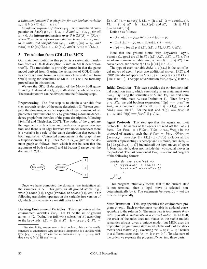
a valuation function V is given by: for any boolean variablex, x ∈ V (s) iff s(x) = true. 2
An infinite sequence of states s0s1... is an initialized com-putation of M(S) if s0 ∈ I , sk ∈ S and sk → sk+1 for allk ≥ 0. An interpreted system over S is IS(S) = (R, π),where R is the set of runs such that each run r correspondsto an initialized computation s0s1... with re(m) = sm, andri(m) = Oi(s0)Oi(s1) . . . Oi(sm); and π(r,m) = V (sm).
3 Translation from GDL-II to MCK
Our main contribution in this paper is a systematic transla-tion from a GDL-II description G into an MCK descriptiontrs(G). The translation is provably correct in that the gamemodel derived from G using the semantics of GDL-II satis-fies the exact same formulas as the model that is derived fromtrs(G) using the semantics of MCK. This will be formallyproved later in this section.
We use the GDL-II description of the Monty Hall gamefrom Fig. 1, denoted as GMH , to illustrate the whole process.The translation trs can be divided into the following steps.
Preprocessing The first step is to obtain a variable-free(i.e., ground) version of the game descriptionG. We can com-pute the domains, or rather supersets of the domains, of allpredicates and functions of G by generating a domain depen-dency graph from the rules of the game description, following[Schiffel and Thielscher, 2007]. The nodes of the graph arethe arguments of functions and predicates in game descrip-tion, and there is an edge between two nodes whenever thereis a variable in a rule of the game description that occurs inboth arguments. Connected components in the graph sharea (super-)domain. E.g., lines 2–6 in GMH give us the do-main graph as follows, from which it can be seen that thearguments of both closed() and hide car() range over thedomain 1, 2, 3.
hide_car(?d)
1
2
3
closed(?d)
Once we have computed the domains, we instantiate allthe variables in G. This gives us all ground atoms, e.g.,true(closed(1)), legal(random, hide car(1)), etc. Ourfollowing translation operates on the variable-free version ofG, which for convenience we still refer to as G.
Deriving Environment Variables This step derives all theenvironment variables Vare. Let AT be the set of groundatoms in G. Define the following subsets of AT accordingto the keywords: ATt = h ∈ AT | h = true(p), ATn =
2For simplicity, we assume x is a boolean; this can be easilyextended to enumerated type variables. Suppose x is a variable withtype e1, . . . , em, we can use m booleans x.e1, . . . , x.em suchthat x.ek ∈ V (s) iff s(x) = ek.
h ∈ AT | h = next(p), ATd = h ∈ AT | h = does(i, a),ATi = h ∈ AT | h = init(p) and ATs = h ∈ AT |h = sees(r, p).
Define t as follows:
• t(true(p)) = pold and t(next(p)) = p;
• t(init(p)) = p, and t(does(i, a)) = did i;
• t(p) = p for all p ∈ AT \ (ATt ∪ ATn ∪ ATd ∪ ATi).
Note that the ground atoms with keywords legal,terminal, goal are all in AT\ (ATt∪ATn∪ATd∪ATi). Theset of environment variable Vare is then t(p) | p ∈ AT. Forconvenience, we denote t(A) as t(x) | x ∈ A.
The type of each variable did i ∈ t(ATd) is the set of le-gal moves of agent i plus two additional moves, INIT andSTOP, that do not appear in G, i.e., a | legal(i, a) ∈ AT ∪INIT, STOP. The type of variables in Vare\t(ATd) is Bool.
Initial Condition This step specifies the environment ini-tial condition Inite, which essentially is an assignment overVare. By using the semantics of G and ATi, we first com-pute the initial state s0 (see Definition 1). Then for anyp ∈ ATi, we add boolean expression “t(p) == true” toInite as a conjunct; and for all did i ∈ t(ATd), we add“did i == INIT”. For the rest, add “t(p) == true” ifp ∈ s0, and “t(p) == false” if p 6∈ s0.
Agent Protocols This step specifies the agents and theirprotocols. The names of the agents are read off the role()facts. Let Prot i = (PVar i,OVar i,Actsi,Prog i) be theprotocol of agent i, such that PVar i = Vare, OVar i =sees i p | sees i p ∈ t(ATs) ∪ did i includes all thevariables representing i’s percept and i’s move, and Actsi =a | legal(i, a) ∈ G includes all the legal moves of agenti. Note that Actsi does not include the two special moves inthe protocol. The last componentProg i is a standard programof the following format:
b e g i n do neg t e r m i n a l −>i f l e g a l i a 1 −> <<a1>> [ ]
l e g a l i a 2 −> <<a2>> [ ]. . .
f iod end
This program intuitively means that if the current stateis not terminal, then a legal move is selected non-determinstically by i. The statements between do · · · od areexecuted repeatedly.
State Transition This step specifies the environment pro-gram Proge. Each environment variable is updated corre-sponding to the rules inG. The main task is to translate theserules into MCK statements in a correct order. In GDL-II,the order of the rules does not matter as the stable modelssemantics always gives a unique model, but MCK uses theimperative programming style in which the order of the state-ments does matter; e.g., executing “x := 0;x := 1; ” resultsin a different state than “x := 1;x := 0; ”. To take care ofthe order, we separate the program Proge into three parts.
GIGA'13 Proceedings50
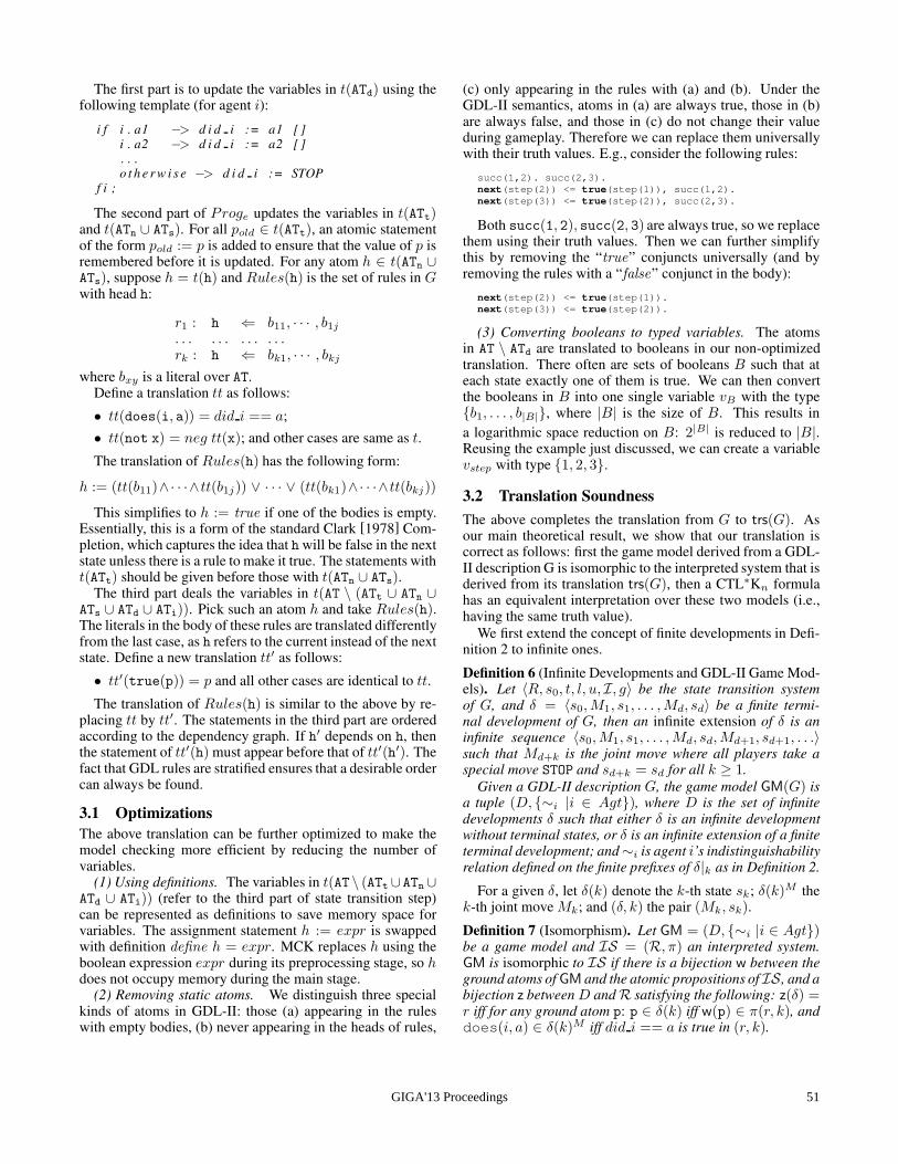
The first part is to update the variables in t(ATd) using thefollowing template (for agent i):
i f i . a1 −> d i d i := a1 [ ]i . a2 −> d i d i := a2 [ ]. . .o t h e r w i s e −> d i d i := STOP
f i ;
The second part of Proge updates the variables in t(ATt)and t(ATn ∪ ATs). For all pold ∈ t(ATt), an atomic statementof the form pold := p is added to ensure that the value of p isremembered before it is updated. For any atom h ∈ t(ATn ∪ATs), suppose h = t(h) and Rules(h) is the set of rules in Gwith head h:
r1 : h ⇐ b11, · · · , b1j. . . . . . . . . . . .rk : h ⇐ bk1, · · · , bkj
where bxy is a literal over AT.Define a translation tt as follows:
• tt(does(i, a)) = did i == a;
• tt(not x) = neg tt(x); and other cases are same as t.
The translation of Rules(h) has the following form:
h := (tt(b11)∧· · ·∧tt(b1j)) ∨ · · · ∨ (tt(bk1)∧· · ·∧tt(bkj))
This simplifies to h := true if one of the bodies is empty.Essentially, this is a form of the standard Clark [1978] Com-pletion, which captures the idea that h will be false in the nextstate unless there is a rule to make it true. The statements witht(ATt) should be given before those with t(ATn ∪ ATs).
The third part deals the variables in t(AT \ (ATt ∪ ATn ∪ATs ∪ ATd ∪ ATi)). Pick such an atom h and take Rules(h).The literals in the body of these rules are translated differentlyfrom the last case, as h refers to the current instead of the nextstate. Define a new translation tt′ as follows:
• tt′(true(p)) = p and all other cases are identical to tt.
The translation of Rules(h) is similar to the above by re-placing tt by tt′. The statements in the third part are orderedaccording to the dependency graph. If h′ depends on h, thenthe statement of tt′(h) must appear before that of tt′(h′). Thefact that GDL rules are stratified ensures that a desirable ordercan always be found.
3.1 Optimizations
The above translation can be further optimized to make themodel checking more efficient by reducing the number ofvariables.
(1) Using definitions. The variables in t(AT\ (ATt∪ATn∪ATd ∪ ATi)) (refer to the third part of state transition step)can be represented as definitions to save memory space forvariables. The assignment statement h := expr is swappedwith definition define h = expr. MCK replaces h using theboolean expression expr during its preprocessing stage, so hdoes not occupy memory during the main stage.
(2) Removing static atoms. We distinguish three specialkinds of atoms in GDL-II: those (a) appearing in the ruleswith empty bodies, (b) never appearing in the heads of rules,
(c) only appearing in the rules with (a) and (b). Under theGDL-II semantics, atoms in (a) are always true, those in (b)are always false, and those in (c) do not change their valueduring gameplay. Therefore we can replace them universallywith their truth values. E.g., consider the following rules:
succ(1,2). succ(2,3).
next(step(2)) <= true(step(1)), succ(1,2).
next(step(3)) <= true(step(2)), succ(2,3).
Both succ(1, 2), succ(2, 3) are always true, so we replacethem using their truth values. Then we can further simplifythis by removing the “true” conjuncts universally (and byremoving the rules with a “false” conjunct in the body):
next(step(2)) <= true(step(1)).
next(step(3)) <= true(step(2)).
(3) Converting booleans to typed variables. The atomsin AT \ ATd are translated to booleans in our non-optimizedtranslation. There often are sets of booleans B such that ateach state exactly one of them is true. We can then convertthe booleans in B into one single variable vB with the typeb1, . . . , b|B|, where |B| is the size of B. This results in
a logarithmic space reduction on B: 2|B| is reduced to |B|.Reusing the example just discussed, we can create a variablevstep with type 1, 2, 3.
3.2 Translation Soundness
The above completes the translation from G to trs(G). Asour main theoretical result, we show that our translation iscorrect as follows: first the game model derived from a GDL-II description G is isomorphic to the interpreted system that isderived from its translation trs(G), then a CTL∗Kn formulahas an equivalent interpretation over these two models (i.e.,having the same truth value).
We first extend the concept of finite developments in Defi-nition 2 to infinite ones.
Definition 6 (Infinite Developments and GDL-II Game Mod-els). Let 〈R, s0, t, l, u, I, g〉 be the state transition systemof G, and δ = 〈s0,M1, s1, . . . ,Md, sd〉 be a finite termi-nal development of G, then an infinite extension of δ is aninfinite sequence 〈s0,M1, s1, . . . ,Md, sd,Md+1, sd+1, . . .〉such that Md+k is the joint move where all players take aspecial move STOP and sd+k = sd for all k ≥ 1.
Given a GDL-II description G, the game model GM(G) isa tuple (D, ∼i |i ∈ Agt), where D is the set of infinitedevelopments δ such that either δ is an infinite developmentwithout terminal states, or δ is an infinite extension of a finiteterminal development; and∼i is agent i’s indistinguishabilityrelation defined on the finite prefixes of δ|k as in Definition 2.
For a given δ, let δ(k) denote the k-th state sk; δ(k)M thek-th joint move Mk; and (δ, k) the pair (Mk, sk).
Definition 7 (Isomorphism). Let GM = (D, ∼i |i ∈ Agt)be a game model and IS = (R, π) an interpreted system.GM is isomorphic to IS if there is a bijection w between theground atoms of GM and the atomic propositions of IS , and abijection z betweenD and R satisfying the following: z(δ) =r iff for any ground atom p: p ∈ δ(k) iff w(p) ∈ π(r, k), anddoes(i, a) ∈ δ(k)M iff did i == a is true in (r, k).
GIGA'13 Proceedings 51
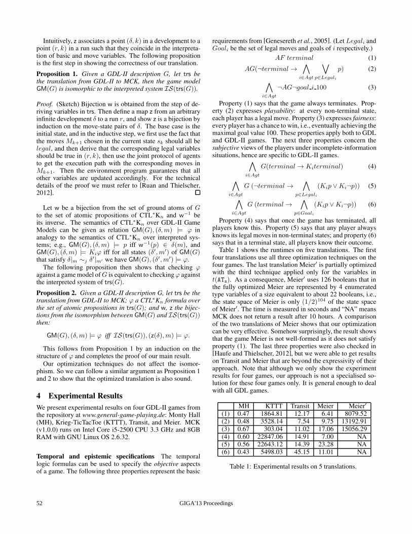
Intuitively, z associates a point (δ, k) in a development to apoint (r, k) in a run such that they coincide in the interpreta-tion of basic and move variables. The following propositionis the first step in showing the correctness of our translation.
Proposition 1. Given a GDL-II description G, let trs bethe translation from GDL-II to MCK, then the game modelGM(G) is isomorphic to the interpreted system IS(trs(G)).
Proof. (Sketch) Bijection w is obtained from the step of de-riving variables in trs. Then define a map z from an arbitraryinfinite development δ to a run r, and show z is a bijection byinduction on the move-state pairs of δ. The base case is theinitial state, and in the inductive step, we first use the fact thatthe moves Mk+1 chosen in the current state sk should all belegal, and then derive that the corresponding legal variablesshould be true in (r, k), then use the joint protocol of agentsto get the execution path with the corresponding moves inMk+1. Then the environment program guarantees that allother variables are updated accordingly. For the technicaldetails of the proof we must refer to [Ruan and Thielscher,2012].
Let w be a bijection from the set of ground atoms of Gto the set of atomic propositions of CTL∗Kn and w
−1 beits inverse. The semantics of CTL∗Kn over GDL-II GameModels can be given as relation GM(G), (δ,m) |= ϕ inanalogy to the semantics of CTL∗Kn over interpreted sys-tems; e.g., GM(G), (δ,m) |= p iff w
−1(p) ∈ δ(m), andGM(G), (δ,m) |= Kiϕ iff for all states (δ′,m′) of GM(G)that satisfy δ|m ∼j δ
′|m′ we have GM(G), (δ′,m′) |= ϕ.
The following proposition then shows that checking ϕagainst a game model ofG is equivalent to checkingϕ againstthe interpreted system of trs(G).
Proposition 2. Given a GDL-II description G, let trs be thetranslation from GDL-II to MCK; ϕ a CTL∗Kn formula overthe set of atomic propositions in trs(G); and w, z the bijec-tions from the isomorphism between GM(G) and IS(trs(G))then:
GM(G), (δ,m) |= ϕ iff IS(trs(G)), (z(δ),m) |= ϕ.
This follows from Proposition 1 by an induction on thestructure of ϕ and completes the proof of our main result.
Our optimization techniques do not affect the isomor-phism. So we can follow a similar argument as Proposition 1and 2 to show that the optimized translation is also sound.
4 Experimental Results
We present experimental results on four GDL-II games fromthe repository at www.general-game-playing.de: Monty Hall(MH), Krieg-TicTacToe (KTTT), Transit, and Meier. MCK(v1.0.0) runs on Intel Core i5-2500 CPU 3.3 GHz and 8GBRAM with GNU Linux OS 2.6.32.
Temporal and epistemic specifications The temporallogic formulas can be used to specify the objective aspectsof a game. The following three properties represent the basic
requirements from [Genesereth et al., 2005]. (Let Legali andGoali be the set of legal moves and goals of i respectively.)
AF terminal (1)
AG(¬terminal →∧
i∈Agt
∨
p∈Legali
p) (2)
∧
i∈Agt
¬AG¬goal i 100 (3)
Property (1) says that the game always terminates. Prop-erty (2) expresses playability: at every non-terminal state,each player has a legal move. Property (3) expresses fairness:every player has a chance to win, i.e., eventually achieving themaximal goal value 100. These properties apply both to GDLand GDL-II games. The next three properties concern thesubjective views of the players under incomplete-informationsituations, hence are specific to GDL-II games.
∧
i∈Agt
G(terminal → Kiterminal) (4)
∧
i∈Agt
G (¬terminal →∧
p∈Legali
(Kip ∨Ki¬p)) (5)
∧
i∈Agt
G (terminal →∧
p∈Goali
(Kip ∨Ki¬p)) (6)
Property (4) says that once the game has terminated, allplayers know this. Property (5) says that any player alwaysknows its legal moves in non-terminal states; and property (6)says that in a terminal state, all players know their outcome.
Table 1 shows the runtimes on five translations. The firstfour translations use all three optimization techniques on thefour games. The last translation Meier′ is partially optimizedwith the third technique applied only for the variables int(ATs). As a consequence, Meier′ uses 126 booleans that inthe fully optimized Meier are represented by 4 enumeratedtype variables of a size equivalent to about 22 booleans, i.e.,the state space of Meier is only (1/2)104 of the state spaceof Meier′. The time is measured in seconds and “NA” meansMCK does not return a result after 10 hours. A comparisonof the two translations of Meier shows that our optimizationcan be very effective. Somehow surprisingly, the result showsthat the game Meier is not well-formed as it does not satisfyproperty (1). The last three properties were also checked in[Haufe and Thielscher, 2012], but we were able to get resultson Transit and Meier that are beyond the expressivity of theirapproach. Note that although we only show the experimentresults for four games, our approach is not a specialised so-lution for these four games only. It is general enough to dealwith all GDL games.
MH KTTT Transit Meier Meier′
(1) 0.47 1864.81 12.17 6.41 8079.52(2) 0.48 3528.14 7.54 9.75 13192.91
(3) 0.67 303.04 11.02 17.06 15056.29
(4) 0.60 22847.06 14.91 7.00 NA(5) 0.56 22643.12 14.39 23.28 NA
(6) 0.43 5498.03 45.15 11.01 NA
Table 1: Experimental results on 5 translations.
GIGA'13 Proceedings52
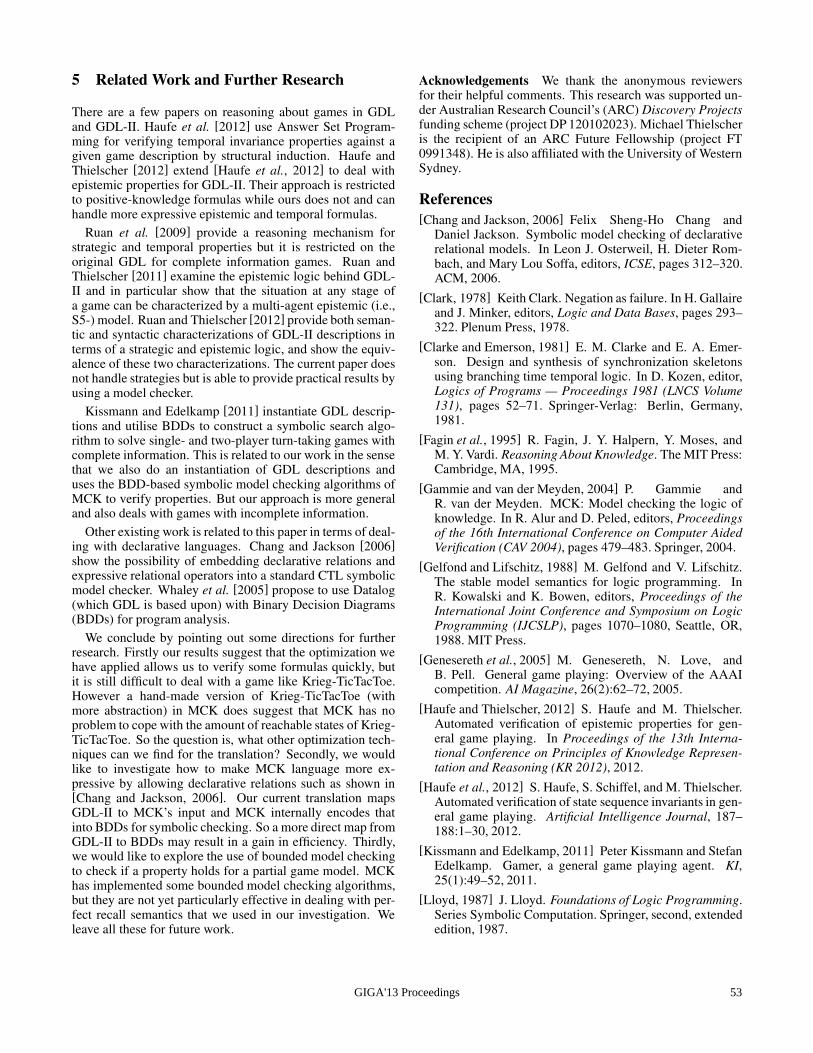
5 Related Work and Further Research
There are a few papers on reasoning about games in GDLand GDL-II. Haufe et al. [2012] use Answer Set Program-ming for verifying temporal invariance properties against agiven game description by structural induction. Haufe andThielscher [2012] extend [Haufe et al., 2012] to deal withepistemic properties for GDL-II. Their approach is restrictedto positive-knowledge formulas while ours does not and canhandle more expressive epistemic and temporal formulas.
Ruan et al. [2009] provide a reasoning mechanism forstrategic and temporal properties but it is restricted on theoriginal GDL for complete information games. Ruan andThielscher [2011] examine the epistemic logic behind GDL-II and in particular show that the situation at any stage ofa game can be characterized by a multi-agent epistemic (i.e.,S5-) model. Ruan and Thielscher [2012] provide both seman-tic and syntactic characterizations of GDL-II descriptions interms of a strategic and epistemic logic, and show the equiv-alence of these two characterizations. The current paper doesnot handle strategies but is able to provide practical results byusing a model checker.
Kissmann and Edelkamp [2011] instantiate GDL descrip-tions and utilise BDDs to construct a symbolic search algo-rithm to solve single- and two-player turn-taking games withcomplete information. This is related to our work in the sensethat we also do an instantiation of GDL descriptions anduses the BDD-based symbolic model checking algorithms ofMCK to verify properties. But our approach is more generaland also deals with games with incomplete information.
Other existing work is related to this paper in terms of deal-ing with declarative languages. Chang and Jackson [2006]
show the possibility of embedding declarative relations andexpressive relational operators into a standard CTL symbolicmodel checker. Whaley et al. [2005] propose to use Datalog(which GDL is based upon) with Binary Decision Diagrams(BDDs) for program analysis.
We conclude by pointing out some directions for furtherresearch. Firstly our results suggest that the optimization wehave applied allows us to verify some formulas quickly, butit is still difficult to deal with a game like Krieg-TicTacToe.However a hand-made version of Krieg-TicTacToe (withmore abstraction) in MCK does suggest that MCK has noproblem to cope with the amount of reachable states of Krieg-TicTacToe. So the question is, what other optimization tech-niques can we find for the translation? Secondly, we wouldlike to investigate how to make MCK language more ex-pressive by allowing declarative relations such as shown in[Chang and Jackson, 2006]. Our current translation mapsGDL-II to MCK’s input and MCK internally encodes thatinto BDDs for symbolic checking. So a more direct map fromGDL-II to BDDs may result in a gain in efficiency. Thirdly,we would like to explore the use of bounded model checkingto check if a property holds for a partial game model. MCKhas implemented some bounded model checking algorithms,but they are not yet particularly effective in dealing with per-fect recall semantics that we used in our investigation. Weleave all these for future work.
Acknowledgements We thank the anonymous reviewersfor their helpful comments. This research was supported un-der Australian Research Council’s (ARC) Discovery Projectsfunding scheme (project DP 120102023). Michael Thielscheris the recipient of an ARC Future Fellowship (project FT0991348). He is also affiliated with the University of WesternSydney.
References
[Chang and Jackson, 2006] Felix Sheng-Ho Chang andDaniel Jackson. Symbolic model checking of declarativerelational models. In Leon J. Osterweil, H. Dieter Rom-bach, and Mary Lou Soffa, editors, ICSE, pages 312–320.ACM, 2006.
[Clark, 1978] Keith Clark. Negation as failure. In H. Gallaireand J. Minker, editors, Logic and Data Bases, pages 293–322. Plenum Press, 1978.
[Clarke and Emerson, 1981] E. M. Clarke and E. A. Emer-son. Design and synthesis of synchronization skeletonsusing branching time temporal logic. In D. Kozen, editor,Logics of Programs — Proceedings 1981 (LNCS Volume131), pages 52–71. Springer-Verlag: Berlin, Germany,1981.
[Fagin et al., 1995] R. Fagin, J. Y. Halpern, Y. Moses, andM. Y. Vardi. Reasoning About Knowledge. The MIT Press:Cambridge, MA, 1995.
[Gammie and van der Meyden, 2004] P. Gammie andR. van der Meyden. MCK: Model checking the logic ofknowledge. In R. Alur and D. Peled, editors, Proceedingsof the 16th International Conference on Computer AidedVerification (CAV 2004), pages 479–483. Springer, 2004.
[Gelfond and Lifschitz, 1988] M. Gelfond and V. Lifschitz.The stable model semantics for logic programming. InR. Kowalski and K. Bowen, editors, Proceedings of theInternational Joint Conference and Symposium on LogicProgramming (IJCSLP), pages 1070–1080, Seattle, OR,1988. MIT Press.
[Genesereth et al., 2005] M. Genesereth, N. Love, andB. Pell. General game playing: Overview of the AAAIcompetition. AI Magazine, 26(2):62–72, 2005.
[Haufe and Thielscher, 2012] S. Haufe and M. Thielscher.Automated verification of epistemic properties for gen-eral game playing. In Proceedings of the 13th Interna-tional Conference on Principles of Knowledge Represen-tation and Reasoning (KR 2012), 2012.
[Haufe et al., 2012] S. Haufe, S. Schiffel, and M. Thielscher.Automated verification of state sequence invariants in gen-eral game playing. Artificial Intelligence Journal, 187–188:1–30, 2012.
[Kissmann and Edelkamp, 2011] Peter Kissmann and StefanEdelkamp. Gamer, a general game playing agent. KI,25(1):49–52, 2011.
[Lloyd, 1987] J. Lloyd. Foundations of Logic Programming.Series Symbolic Computation. Springer, second, extendededition, 1987.
GIGA'13 Proceedings 53
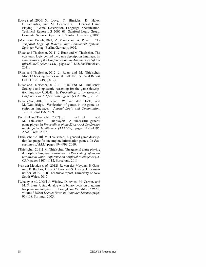
[Love et al., 2006] N. Love, T. Hinrichs, D. Haley,E. Schkufza, and M. Genesereth. General GamePlaying: Game Description Language Specification.Technical Report LG–2006–01, Stanford Logic Group,Computer Science Department, Stanford University, 2006.
[Manna and Pnueli, 1992] Z. Manna and A. Pnueli. TheTemporal Logic of Reactive and Concurrent Systems.Springer-Verlag: Berlin, Germany, 1992.
[Ruan and Thielscher, 2011] J. Ruan and M. Thielscher. Theepistemic logic behind the game description language. InProceedings of the Conference on the Advancement of Ar-tificial Intelligence (AAAI), pages 840–845, San Francisco,2011.
[Ruan and Thielscher, 2012] J. Ruan and M. Thielscher.Model Checking Games in GDL-II: the Technical ReportCSE-TR-201219, (2012)
[Ruan and Thielscher, 2012] J. Ruan and M. Thielscher.Strategic and epistemic reasoning for the game descrip-tion language GDL-II. In Proceedings of the EuropeanConference on Artificial Intelligence (ECAI 2012), 2012.
[Ruan et al., 2009] J. Ruan, W. van der Hoek, andM. Wooldridge. Verification of games in the game de-scription language. Journal Logic and Computation,19(6):1127–1156, 2009.
[Schiffel and Thielscher, 2007] S. Schiffel andM. Thielscher. Fluxplayer: A successful generalgame player. In Proceedings of the 22nd AAAI Conferenceon Artificial Intelligence (AAAI-07), pages 1191–1196.AAAI Press, 2007.
[Thielscher, 2010] M. Thielscher. A general game descrip-tion language for incomplete information games. In Pro-ceedings of AAAI, pages 994–999, 2010.
[Thielscher, 2011] M. Thielscher. The general game playingdescription language is universal. In Proceedings of the In-ternational Joint Conference on Artificial Intelligence (IJ-CAI), pages 1107–1112, Barcelona, 2011.
[van der Meyden et al., 2012] R. van der Meyden, P. Gam-mie, K. Baukus, J. Lee, C. Luo, and X. Huang. User man-ual for MCK 1.0.0. Technical report, University of NewSouth Wales, 2012.
[Whaley et al., 2005] J. Whaley, D. Avots, M. Carbin, andM. S. Lam. Using datalog with binary decision diagramsfor program analysis. In Kwangkeun Yi, editor, APLAS,volume 3780 of Lecture Notes in Computer Science, pages97–118. Springer, 2005.
GIGA'13 Proceedings54
Comparison of GDL Reasoners ∗
Yngvi Bjornsson and Stephan SchiffelSchool of Computer Science / CADIA
Reykjavik University, Icelandyngvi,[email protected]
AbstractThe variety of open-source GDL reasoners avail-able to newcomers to General Game Playing (GGP)lowers the technical barrier of entering the field.This variety, however, also makes it more compli-cated to decide on a fitting reasoner for a givenGGP project, considering the project’s objectives,ambitions, and technical constraints. This papergives an overview of available GDL reasoners, dis-cusses their main pros and cons, and most im-portantly quantifies their relative reasoning perfor-mance on a number of games (in terms of nodessearched per second), showing an order of magni-tude difference in some cases. We similarly quan-tify the performance difference between game-playing systems specifically designed for playinga single game on the one hand and general game-playing systems on the other, witnessing up to sev-eral orders of magnitude difference.
1 IntroductionGames have played an important role as a testbed for ad-vancements in the field of artificial intelligence ever sinceits inception. The focus was initially on developing gen-eral problem-solving systems, but gradually shifted towardsbuilding specialized high-performance game-playing systemscapable of matching wits with the best humans. These highlyspecialized systems were engineered and optimized towardsplaying a single particular game at a world-class level. Ex-amples of such game-playing systems achieving fame areCHINOOK (checkers), DEEPBLUE (chess), and LOGISTELLO(Othello) [Schaeffer and van den Herik, 2002].
The auspicious effect of increased computing speed wasrecognized early as deeper lookahead could greatly improveprograms’ playing strength. Thus, in addition to develop-ing pure algorithmic enhancements much effort was investedin developing compact and efficient data-structures and in-ventive code optimization tricks for the games at hand (asa case in point, ”magic bitboards” in chess allow the boardrepresentation to be transformed from being row-aligned to
∗The support of the Icelandic Centre for Research (RANNIS) isacknowledged.
diagonally-aligned simply by performing a couple of care-fully chosen multiplications — an extremely useful fea-ture for efficiently generating the legal moves of the slidingpieces). It is not uncommon for specialized game-playingprograms to explore millions of nodes per second (nps) onmodern computer hardware, even on a single CPU. Massiveparallel processing has the potential of scaling this alreadyimpressive performance up by a few orders of magnitude.
The International General Game Playing Competi-tion [Genesereth et al., 2005] renewed interest in more gen-eral approaches to computer game playing. In General GamePlaying (GGP), as opposed to creating highly-efficient game-playing agents for playing one specific game, the goal is tocreate agents capable of autonomously learning how to playa wide variety of games skillfully. The games can take var-ious disparate shapes and forms. The principal game rules,such as what the goal of the game is and how the piecesmove, are communicated to the GGP agents using a languagecalled Game Description Language (GDL). The responsi-bility is then on the agents to learn —without any humanintervention— strategies for playing that game well. Obvi-ously such general game-playing systems cannot be expectedto achieve the same level of performance as their game-specific counterparts. It is nonetheless important for them tobe as efficient as possible, not the least because the learningand reasoning mainly takes place in real-time during play.
In GGP, as any other new research field, it is importantto attract new practitioner. One potential obstacle of entry isthe sizable software infrastructure needed for having simply afunctional GGP agent. Fortunately, the community providessoftware tools for lowering this technical barrier. For exam-ple, there are several open-source GGP agents available, on-line game servers for playing other agents, as well as variousGDL reasoners that can be plugged directly into new projects.This frees newcomers from having to implement their ownGDL interpreters, allowing them instead to concentrate onany of the other challenging aspects of GGP.
In this paper we give an overview of available GDL rea-soners, discuss their main pros and cons, and quantify theirrelative reasoning efficiency on a number of games. We hopethat this work not only provides added insights into how tofurther improve GDL reasoners’ efficiency, but also makesit easier for both new and old GGP practitioners to select aproper reasoner for their projects or tasks at hand. We fur-
GIGA'13 Proceedings 55
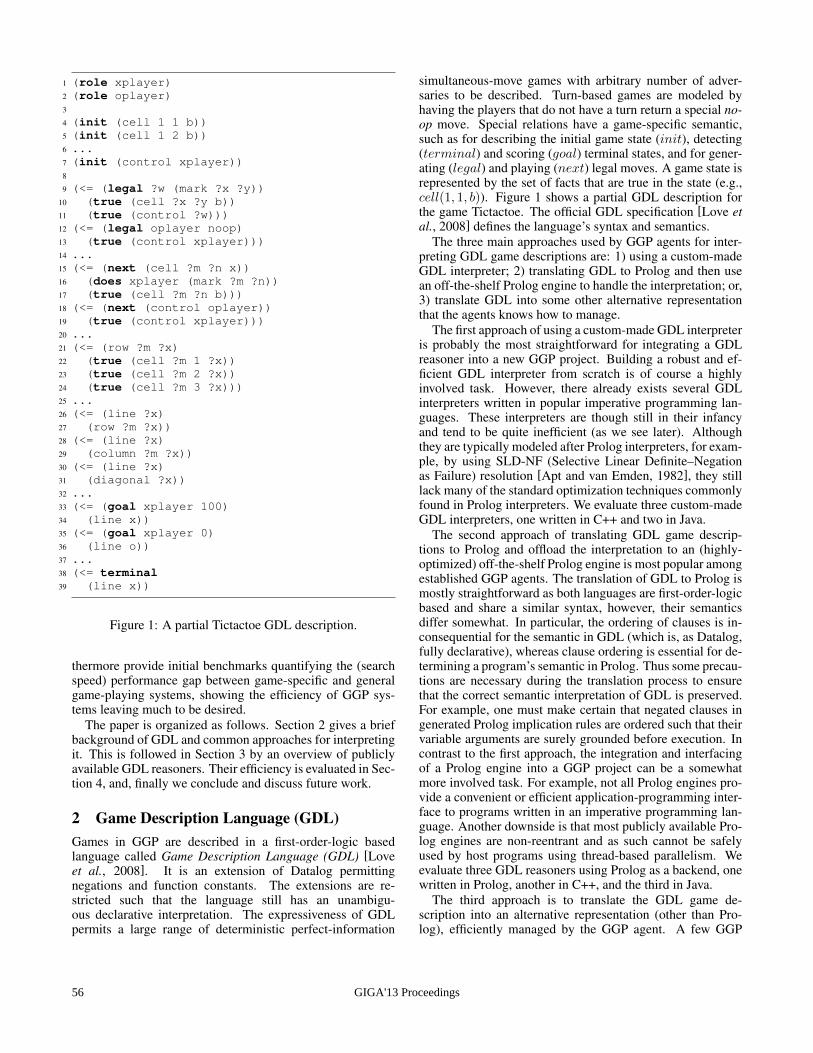
1 (role xplayer)2 (role oplayer)3
4 (init (cell 1 1 b))5 (init (cell 1 2 b))6 ...7 (init (control xplayer))8
9 (<= (legal ?w (mark ?x ?y))10 (true (cell ?x ?y b))11 (true (control ?w)))12 (<= (legal oplayer noop)13 (true (control xplayer)))14 ...15 (<= (next (cell ?m ?n x))16 (does xplayer (mark ?m ?n))17 (true (cell ?m ?n b)))18 (<= (next (control oplayer))19 (true (control xplayer)))20 ...21 (<= (row ?m ?x)22 (true (cell ?m 1 ?x))23 (true (cell ?m 2 ?x))24 (true (cell ?m 3 ?x)))25 ...26 (<= (line ?x)27 (row ?m ?x))28 (<= (line ?x)29 (column ?m ?x))30 (<= (line ?x)31 (diagonal ?x))32 ...33 (<= (goal xplayer 100)34 (line x))35 (<= (goal xplayer 0)36 (line o))37 ...38 (<= terminal39 (line x))
Figure 1: A partial Tictactoe GDL description.
thermore provide initial benchmarks quantifying the (searchspeed) performance gap between game-specific and generalgame-playing systems, showing the efficiency of GGP sys-tems leaving much to be desired.
The paper is organized as follows. Section 2 gives a briefbackground of GDL and common approaches for interpretingit. This is followed in Section 3 by an overview of publiclyavailable GDL reasoners. Their efficiency is evaluated in Sec-tion 4, and, finally we conclude and discuss future work.
2 Game Description Language (GDL)Games in GGP are described in a first-order-logic basedlanguage called Game Description Language (GDL) [Loveet al., 2008]. It is an extension of Datalog permittingnegations and function constants. The extensions are re-stricted such that the language still has an unambigu-ous declarative interpretation. The expressiveness of GDLpermits a large range of deterministic perfect-information
simultaneous-move games with arbitrary number of adver-saries to be described. Turn-based games are modeled byhaving the players that do not have a turn return a special no-op move. Special relations have a game-specific semantic,such as for describing the initial game state (init), detecting(terminal) and scoring (goal) terminal states, and for gener-ating (legal) and playing (next) legal moves. A game state isrepresented by the set of facts that are true in the state (e.g.,cell(1, 1, b)). Figure 1 shows a partial GDL description forthe game Tictactoe. The official GDL specification [Love etal., 2008] defines the language’s syntax and semantics.
The three main approaches used by GGP agents for inter-preting GDL game descriptions are: 1) using a custom-madeGDL interpreter; 2) translating GDL to Prolog and then usean off-the-shelf Prolog engine to handle the interpretation; or,3) translate GDL into some other alternative representationthat the agents knows how to manage.
The first approach of using a custom-made GDL interpreteris probably the most straightforward for integrating a GDLreasoner into a new GGP project. Building a robust and ef-ficient GDL interpreter from scratch is of course a highlyinvolved task. However, there already exists several GDLinterpreters written in popular imperative programming lan-guages. These interpreters are though still in their infancyand tend to be quite inefficient (as we see later). Althoughthey are typically modeled after Prolog interpreters, for exam-ple, by using SLD-NF (Selective Linear Definite–Negationas Failure) resolution [Apt and van Emden, 1982], they stilllack many of the standard optimization techniques commonlyfound in Prolog interpreters. We evaluate three custom-madeGDL interpreters, one written in C++ and two in Java.
The second approach of translating GDL game descrip-tions to Prolog and offload the interpretation to an (highly-optimized) off-the-shelf Prolog engine is most popular amongestablished GGP agents. The translation of GDL to Prolog ismostly straightforward as both languages are first-order-logicbased and share a similar syntax, however, their semanticsdiffer somewhat. In particular, the ordering of clauses is in-consequential for the semantic in GDL (which is, as Datalog,fully declarative), whereas clause ordering is essential for de-termining a program’s semantic in Prolog. Thus some precau-tions are necessary during the translation process to ensurethat the correct semantic interpretation of GDL is preserved.For example, one must make certain that negated clauses ingenerated Prolog implication rules are ordered such that theirvariable arguments are surely grounded before execution. Incontrast to the first approach, the integration and interfacingof a Prolog engine into a GGP project can be a somewhatmore involved task. For example, not all Prolog engines pro-vide a convenient or efficient application-programming inter-face to programs written in an imperative programming lan-guage. Another downside is that most publicly available Pro-log engines are non-reentrant and as such cannot be safelyused by host programs using thread-based parallelism. Weevaluate three GDL reasoners using Prolog as a backend, onewritten in Prolog, another in C++, and the third in Java.
The third approach is to translate the GDL game de-scription into an alternative representation (other than Pro-log), efficiently managed by the GGP agent. A few GGP
GIGA'13 Proceedings56
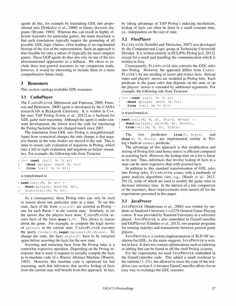
agents do this, for example by translating GDL into propo-sitional nets [Schkufza et al., 2008] or binary decision dia-grams [Bryant, 1985]. Whereas this can result in highly ef-ficient reasoners for particular games, the main drawback isthat such translations typically require the grounding of allpossible GDL logic clauses, often leading to an exponentialblowup of the size of the representation. Such an approach isthus feasible for only a subset of (typically the more simpler)games. These GGP agents do thus also rely on one of the twoaforementioned approaches as a fallback. We chose to ex-clude these non-general reasoners in our comparison study;however, it would be interesting to include them in a morecomprehensive future study.
3 ReasonersThis section catalogs available GDL reasoners.
3.1 CadiaPlayerThe CADIAPLAYER [Bjornsson and Finnsson, 2009; Finns-son and Bjornsson, 2008] agent is developed by the CADIAresearch lab at Reykjavik University. It is written in C++,but uses YAP Prolog [Costa et al., 2012] as a backend forGDL game state reasoning. Although the agent is under con-stant development, the lowest level the code for interfacingthe Prolog backend has not changed much since 2007.
The translation from GDL into Prolog is straightforward:Apart from syntactical changes the only change is that nega-tive literals in the rules bodies are moved to the end. This isdone to ensure safe evaluation of negations in Prolog, whichuses a left to right evaluation and negation-as-failure seman-tics. For example, the following rule from Tictactoe
1 (<= (next (cell ?m ?n x))2 (does xplayer (mark ?m ?n))3 (true (cell ?m ?n b)))
is transformed to
1 next(cell(M, N, x)) :-2 does(xplayer, mark(M, N)),3 state(cell(M, N, b)).
As a consequence, these Prolog rules can only be usedto reason about one particular state at a time. To set thisstate, facts of the form state(F) are asserted in Prolog –one for each fluent F in the current state. Similarly, to setthe moves that the players have done, CADIAPLAYER as-serts facts of the form does(R,M). This allows to reasonabout the game. For example, to compute the legal movesof xplayer in the current state, CADIAPLAYER executesthe query findall(M,legal(xplayer,M),Moves). Tochange the state, the facts state(F) have to be retractedagain before asserting the facts for the new state.
Asserting and retracting facts from the Prolog rules is asomewhat expensive operation. Depending on the Prolog in-terpreter that is used, it requires to actually compile the factsin to machine code of a Warren Abstract Machine [Warren,1983]. However, this machine code is optimized for fastreasoning, such that inferences that involve lookup of factsfrom the current state will benefit from this approach. In fact,
by taking advantage of YAP Prolog’s indexing mechanism,lookup of facts can often be done in a small constant time,i.e., independent on the size of state.
3.2 FluxPlayerFLUXPLAYER [Schiffel and Thielscher, 2007] was developedby the Computational Logic group at Technische UniversitatDresden. It is written entirely in ECLiPSe Prolog [ecl, 2013],except for a small part handling the communication which iswritten in Java.
Consequently, FLUXPLAYER also converts the GDL rulesinto Prolog. However, the approach differs from CADIA-PLAYER’s by not needing to assert and retract facts. Insteadstates and players’ moves are modeled as Prolog lists. Eachpredicate in the game rules that depends on the state or onthe players’ moves is extended by additional arguments. Forexample, the following rule from Tictactoe
1 (<= (next (cell ?m ?n x))2 (does xplayer (mark ?m ?n))3 (true (cell ?m ?n b)))
is transformed to
1 next(cell(M, N, x), State, Moves) :-2 does(xplayer, mark(M, N), Moves),3 true(cell(M, N, b), State).
The two predicates true(F, State) anddoes(R, M, Moves) are implemented similar to Pro-log’s built-in member predicate.
The advantage of this approach is that modification andstoring of Prolog lists (and hence states) is efficient comparedto asserting facts. However, the lookup time on a list is linearin its size. Thus, inferences that involve lookup of facts in astate can be more expensive than with asserted facts.
In addition to this standard transformation of GDL rulesinto Prolog rules, FLUXPLAYER comes with a multitude ofgame analysis algorithms (see, e.g., [Haufe et al., 2012;2011]), some of which are used to modify the game rules todecrease inference time. In the interest of a fair comparisonof the reasoners, these improvements were turned off for theexperiments presented in this paper.
3.3 JavaProverJAVAPROVER [Halderman et al., 2006] was written by stu-dents in Stanford University’s cs227b General Game Playingcourse. It was provided by Stanford University as a referenceplayer. JAVAPROVER is also embedded in GameControllerand GGPServer [Gunther et al., 2013], two popular programsfor running matches and tournaments between general gameplayers.
JAVAPROVER is a custom implementation of SLD-NF res-olution for GDL. As the name suggests, JAVAPROVER is writ-ten in Java. It does not contain optimizations such as indexingor tabling that can be found in off-the-shelf Prolog systems.
For the experiments we used JAVAPROVER embedded inthe GameController code. This added a small overhead tothe runtime (1–2%), but allowed to reuse the code of the test-driver (see section 4.1) because GameController allows for aneasy way to exchange the GDL reasoner.
GIGA'13 Proceedings 57
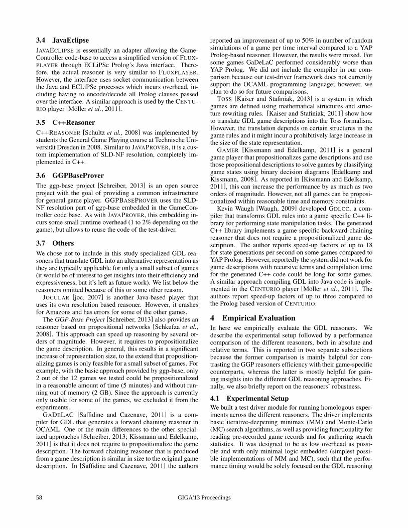
3.4 JavaEclipseJAVAECLIPSE is essentially an adapter allowing the Game-Controller code-base to access a simplified version of FLUX-PLAYER through ECLiPSe Prolog’s Java interface. There-fore, the actual reasoner is very similar to FLUXPLAYER.However, the interface uses socket communication betweenthe Java and ECLiPSe processes which incurs overhead, in-cluding having to encode/decode all Prolog clauses passedover the interface. A similar approach is used by the CENTU-RIO player [Moller et al., 2011].
3.5 C++ReasonerC++REASONER [Schultz et al., 2008] was implemented bystudents the General Game Playing course at Technische Uni-versitat Dresden in 2008. Similar to JAVAPROVER, it is a cus-tom implementation of SLD-NF resolution, completely im-plemented in C++.
3.6 GGPBaseProverThe ggp-base project [Schreiber, 2013] is an open sourceproject with the goal of providing a common infrastructurefor general game player. GGPBASEPROVER uses the SLD-NF resolution part of ggp-base embedded in the GameCon-troller code base. As with JAVAPROVER, this embedding in-curs some small runtime overhead (1 to 2% depending on thegame), but allows to reuse the code of the test-driver.
3.7 OthersWe chose not to include in this study specialized GDL rea-soners that translate GDL into an alternative representation asthey are typically applicable for only a small subset of games(it would be of interest to get insights into their efficiency andexpressiveness, but it’s left as future work). We list below thereasoners omitted because of this or some other reason.
JOCULAR [joc, 2007] is another Java-based player thatuses its own resolution based reasoner. However, it crashesfor Amazons and has errors for some of the other games.
The GGP-Base Project [Schreiber, 2013] also provides anreasoner based on propositional networks [Schkufza et al.,2008]. This approach can speed up reasoning by several or-ders of magnitude. However, it requires to propositionalizethe game description. In general, this results in a significantincrease of representation size, to the extend that proposition-alizing games is only feasible for a small subset of games. Forexample, with the basic approach provided by ggp-base, only2 out of the 12 games we tested could be propositionalizedin a reasonable amount of time (5 minutes) and without run-ning out of memory (2 GB). Since the approach is currentlyonly usable for some of the games, we excluded it from theexperiments.
GADELAC [Saffidine and Cazenave, 2011] is a com-piler for GDL that generates a forward chaining reasoner inOCAML. One of the main differences to the other special-ized approaches [Schreiber, 2013; Kissmann and Edelkamp,2011] is that it does not require to propositionalize the gamedescription. The forward chaining reasoner that is producedfrom a game description is similar in size to the original gamedescription. In [Saffidine and Cazenave, 2011] the authors
reported an improvement of up to 50% in number of randomsimulations of a game per time interval compared to a YAPProlog-based reasoner. However, the results were mixed. Forsome games GaDeLaC performed considerably worse thanYAP Prolog. We did not include the compiler in our com-parison because our test-driver framework does not currentlysupport the OCAML programming language; however, weplan to do so for future comparisons.
TOSS [Kaiser and Stafiniak, 2013] is a system in whichgames are defined using mathematical structures and struc-ture rewriting rules. [Kaiser and Stafiniak, 2011] show howto translate GDL game descriptions into the Toss formalism.However, the translation depends on certain structures in thegame rules and it might incur a prohibitively large increase inthe size of the state representation.
GAMER [Kissmann and Edelkamp, 2011] is a generalgame player that propositionalizes game descriptions and usethose propositional descriptions to solve games by classifyinggame states using binary decision diagrams [Edelkamp andKissmann, 2008]. As reported in [Kissmann and Edelkamp,2011], this can increase the performance by as much as twoorders of magnitude. However, not all games can be proposi-tionalized within reasonable time and memory constraints.
Kevin Waugh [Waugh, 2009] developed GDLCC, a com-piler that transforms GDL rules into a game specific C++ li-brary for performing state manipulation tasks. The generatedC++ library implements a game specific backward-chainingreasoner that does not require a propositionalized game de-scription. The author reports speed-up factors of up to 18for state generations per second on some games compared toYAP Prolog. However, reportedly the system did not work forgame descriptions with recursive terms and compilation timefor the generated C++ code could be long for some games.A similar approach compiling GDL into Java code is imple-mented in the CENTURIO player [Moller et al., 2011]. Theauthors report speed-up factors of up to three compared tothe Prolog based version of CENTURIO.
4 Empirical EvaluationIn here we empirically evaluate the GDL reasoners. Wedescribe the experimental setup followed by a performancecomparison of the different reasoners, both in absolute andrelative terms. This is reported in two separate subsectionsbecause the former comparison is mainly helpful for con-trasting the GGP reasoners efficiency with their game-specificcounterparts, whereas the latter is mostly helpful for gain-ing insights into the different GDL reasoning approaches. Fi-nally, we also briefly report on the reasoners’ robustness.
4.1 Experimental SetupWe built a test driver module for running homologous exper-iments across the different reasoners. The driver implementsbasic iterative-deepening minimax (MM) and Monte-Carlo(MC) search algorithms, as well as providing functionality forreading pre-recorded game records and for gathering searchstatistics. It was designed to be as low overhead as possi-ble and with only minimal logic embedded (simplest possi-ble implementations of MM and MC), such that the perfor-mance timing would be solely focused on the GDL reasoning
GIGA'13 Proceedings58
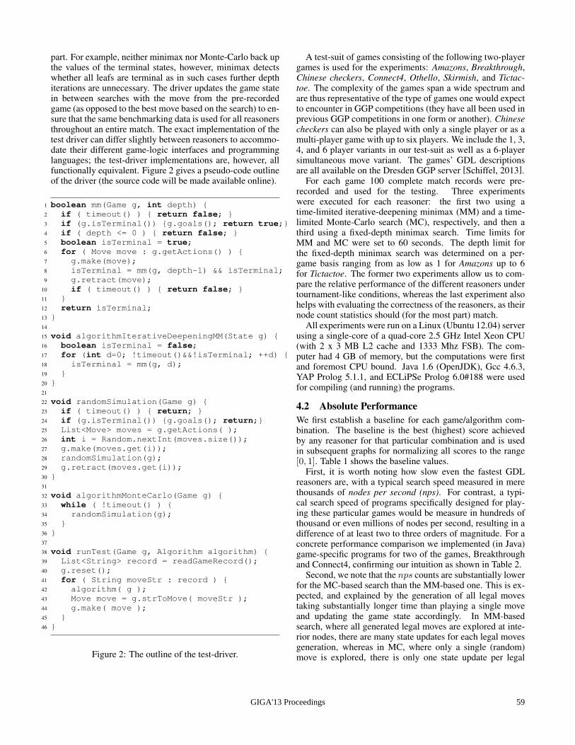
part. For example, neither minimax nor Monte-Carlo back upthe values of the terminal states, however, minimax detectswhether all leafs are terminal as in such cases further depthiterations are unnecessary. The driver updates the game statein between searches with the move from the pre-recordedgame (as opposed to the best move based on the search) to en-sure that the same benchmarking data is used for all reasonersthroughout an entire match. The exact implementation of thetest driver can differ slightly between reasoners to accommo-date their different game-logic interfaces and programminglanguages; the test-driver implementations are, however, allfunctionally equivalent. Figure 2 gives a pseudo-code outlineof the driver (the source code will be made available online).
1 boolean mm(Game g, int depth) 2 if ( timeout() ) return false; 3 if (g.isTerminal()) g.goals(); return true;4 if ( depth <= 0 ) return false; 5 boolean isTerminal = true;6 for ( Move move : g.getActions() ) 7 g.make(move);8 isTerminal = mm(g, depth-1) && isTerminal;9 g.retract(move);
10 if ( timeout() ) return false; 11 12 return isTerminal;13 14
15 void algorithmIterativeDeepeningMM(State g) 16 boolean isTerminal = false;17 for (int d=0; !timeout()&&!isTerminal; ++d) 18 isTerminal = mm(g, d);19 20 21
22 void randomSimulation(Game g) 23 if ( timeout() ) return; 24 if (g.isTerminal()) g.goals(); return;25 List<Move> moves = g.getActions( );26 int i = Random.nextInt(moves.size());27 g.make(moves.get(i));28 randomSimulation(g);29 g.retract(moves.get(i));30 31
32 void algorithmMonteCarlo(Game g) 33 while ( !timeout() ) 34 randomSimulation(g);35 36 37
38 void runTest(Game g, Algorithm algorithm) 39 List<String> record = readGameRecord();40 g.reset();41 for ( String moveStr : record ) 42 algorithm( g );43 Move move = g.strToMove( moveStr );44 g.make( move );45 46
Figure 2: The outline of the test-driver.
A test-suit of games consisting of the following two-playergames is used for the experiments: Amazons, Breakthrough,Chinese checkers, Connect4, Othello, Skirmish, and Tictac-toe. The complexity of the games span a wide spectrum andare thus representative of the type of games one would expectto encounter in GGP competitions (they have all been used inprevious GGP competitions in one form or another). Chinesecheckers can also be played with only a single player or as amulti-player game with up to six players. We include the 1, 3,4, and 6 player variants in our test-suit as well as a 6-playersimultaneous move variant. The games’ GDL descriptionsare all available on the Dresden GGP server [Schiffel, 2013].
For each game 100 complete match records were pre-recorded and used for the testing. Three experimentswere executed for each reasoner: the first two using atime-limited iterative-deepening minimax (MM) and a time-limited Monte-Carlo search (MC), respectively, and then athird using a fixed-depth minimax search. Time limits forMM and MC were set to 60 seconds. The depth limit forthe fixed-depth minimax search was determined on a per-game basis ranging from as low as 1 for Amazons up to 6for Tictactoe. The former two experiments allow us to com-pare the relative performance of the different reasoners undertournament-like conditions, whereas the last experiment alsohelps with evaluating the correctness of the reasoners, as theirnode count statistics should (for the most part) match.
All experiments were run on a Linux (Ubuntu 12.04) serverusing a single-core of a quad-core 2.5 GHz Intel Xeon CPU(with 2 x 3 MB L2 cache and 1333 Mhz FSB). The com-puter had 4 GB of memory, but the computations were firstand foremost CPU bound. Java 1.6 (OpenJDK), Gcc 4.6.3,YAP Prolog 5.1.1, and ECLiPSe Prolog 6.0#188 were usedfor compiling (and running) the programs.
4.2 Absolute PerformanceWe first establish a baseline for each game/algorithm com-bination. The baseline is the best (highest) score achievedby any reasoner for that particular combination and is usedin subsequent graphs for normalizing all scores to the range[0, 1]. Table 1 shows the baseline values.
First, it is worth noting how slow even the fastest GDLreasoners are, with a typical search speed measured in merethousands of nodes per second (nps). For contrast, a typi-cal search speed of programs specifically designed for play-ing these particular games would be measure in hundreds ofthousand or even millions of nodes per second, resulting in adifference of at least two to three orders of magnitude. For aconcrete performance comparison we implemented (in Java)game-specific programs for two of the games, Breakthroughand Connect4, confirming our intuition as shown in Table 2.
Second, we note that the nps counts are substantially lowerfor the MC-based search than the MM-based one. This is ex-pected, and explained by the generation of all legal movestaking substantially longer time than playing a single moveand updating the game state accordingly. In MM-basedsearch, where all generated legal moves are explored at inte-rior nodes, there are many state updates for each legal movesgeneration, whereas in MC, where only a single (random)move is explored, there is only one state update per legal
GIGA'13 Proceedings 59
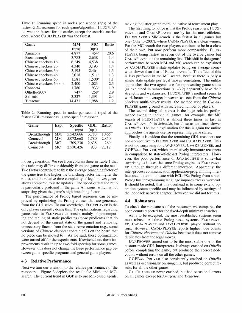
Table 1: Running speed in nodes per second (nps) of thefastest GDL reasoner for each game/algorithm: FLUXPLAY-ER was the fastest for all entries except the asterisk-markedones, where CADIAPLAYER was the fastest.
Game MM MC Ratio(nps) (nps)
Amazons 4,877 454∗ 20.6Breakthrough 3,783 2,638 1.4Chinese checkers 1p 6,249 4,538 1.4Chinese checkers 2p 4,340 3,193 1.4Chinese checkers 3p 3,195 2,464 1.3Chinese checkers 4p 2,018 1,511∗ 1.3Chinese checkers 6p 1,581 1,500∗ 1.1Chinese checkers 6p-sim 2,400 1,023 2.3Connect4 1,780 933∗ 1.9Othello-2007 747∗ 258∗ 2.9Skirmish 3,327 1,391 2.4Tictactoe 14,471 11,988 1.2
Table 2: Running speed in nodes per second (nps) of thefastest GDL reasoner vs. game-specific reasoner.
Game Exp. Specific GDL Ratio(nps) (nps)
Breakthrough MM 5,543,666 3,783 1,465Connect4 MM 5,072,668 1,780 2,850Breakthrough MC 709,230 2,638 269Connect4 MC 2,530,426 933 2,712
moves generation. We see from column three in Table 1 thatthis ratio may differ considerably from one game to the next.Two factors contribute to this: the average branching factor ofthe game tree (the higher the branching factor the higher theratio), and the relative time complexity of legal moves gener-ations compared to state updates. The speed difference ratiois particularly profound in the game Amazons, which is notsurprising given the game’s high branching factor.
The performance of Prolog based reasoners can be im-proved by optimizing the Prolog clauses that are generatedfrom the GDL rules. To our knowledge, FLUXPLAYER is theonly player currently doing this. The optimizations regardinggame rules in FLUXPLAYER consist mainly of precomput-ing and tabling of static predicates (those predicates that donot depend on the current state of the game) and removingunnecessary fluents from the state representation (e.g., someversions of Chinese checkers contain cells on the board thatno piece can be moved to). As we said, these optimizationwere turned off for the experiments. If switched on, these im-provements result in up to two-fold speedup for some games.However, this does not change the huge performance gap be-tween game-specific programs and general game players.
4.3 Relative PerformanceNext we turn our attention to the relative performance of thereasoners. Figure 3 depicts the result for MM- and MC-search. The current trend in GGP is to use MC-based agents,
making the latter graph more indicative of tournament play.The first thing to notice is that the Prolog reasoners, FLUX-
PLAYER and CADIAPLAYER, are by far the most efficient.FLUXPLAYER’s MM-search is the fastest in all games butone (Othello-2007), where CADIAPLAYER is a clear winner.For the MC-search the two players continue to be in a classof their own, but now perform more comparably: FLUX-PLAYER being fastest in seven out of the twelve games butCADIAPLAYER in the remaining five. This shift in the agents’performance between MM and MC search can be explainedby CADIAPLAYER’s state updates being on average some-what slower than that of FLUXPLAYER’s. The effect of thisis less profound in the MC search, because there is only asingle state update per legal moves generation. The unlikeapproaches the two agents use for representing game states(as explained in subsections 3.1–3.2) apparently have theirstrengths and weaknesses. FLUXPLAYER’s method seems towork better on average; however, as seen from the Chinesecheckers multi-player results, the method used in CADIA-PLAYER gains ground with increased number of players.
The second thing of interest is the huge relative perfor-mance swing in individual games, for example, the MCsearch of FLUXPLAYER is almost three times as fast asCADIAPLAYER’s in Skirmish, but close to ten times slowerin Othello. The main explanation for this is again the unlikeapproaches the agents use for representing game states.
Finally, it is evident that the remaining GDL reasoners arenon-competitive to FLUXPLAYER and CADIAPLAYER. Thisis not too surprising for JAVAPROVER, C++REASONER, andGGPBASEPROVER, which are relatively immature reasonersin comparison to state-of-the-art Prolog interpreters. How-ever, the poor performance of JAVAECLIPSE is somewhatsurprising as it uses the same Prolog engine as FLUXPLAY-ER although through a different interface. Apparently, theinter-process communication application-programming inter-face used to communicate with ECLiPSe Prolog from a non-Prolog host programming language imposes excess overhead.It should be noted, that this overhead is to some extend op-eration system specific and may be influenced by settings ofthe loopback network adapter. However, we did not test this.
4.4 RobustnessTo check the robustness of the reasoners we compared thenode counts reported for the fixed-depth minimax searches.
As is to be excepted, the most established systems seemmost robust. All three Prolog-based systems, FLUXPLAY-ER, CADIAPLAYER and JAVAECLIPSE, played without er-rors. However, CADIAPLAYER reports higher node countsfor Chinese checkers and Othello because it does not removeduplicates from the legal moves.
JAVAPROVER turned out to be the most stable one of thecustom-made GDL interpreters. It always crashed on Othellobefore completing the game, but produced the correct nodecounts without errors on all the other games.
GGPBASEPROVER also consistently crashed on Othelloas well as occasionally on Amazons, but produced correct re-sults for all the other games.
C++REASONER never crashed, but had occasional errorson all games except for Amazons and Tictactoe.
GIGA'13 Proceedings60
MM
0.00.20.40.60.81.0
amaz
ons
brea
kthr
ough
c.−
chec
kers
1
c.−
chec
kers
2
c.−
chec
kers
3
c.−
chec
kers
4
c.−
chec
kers
6
c.−
chec
kers
6s
conn
ect4
othe
llo
skir
mis
h
ticta
ctoe
MC
0.00.20.40.60.81.0
fluxplayercadiaplayerjavaeclipsejavaproverggpbaseproverc++reasoner
Figure 3: Running speed in nodes per second relative to the fastest reasoner for each of the games.
5 Conclusions and Future WorkSeveral conclusions can be drawn from this work. We list themain ones and discuss some implications they may have:
• The GDL reasoners are at least two to three orders ofmagnitude slower than their game-specific counterparts.Although one cannot expect generalized approaches tobe quite as efficient as game-specific ones, this huge dif-ference is nonetheless somewhat worrisome. For exam-ple, the slow state-space reasoning does exclude poten-tially interesting search and learning techniques from be-ing effectively applied in GGP — this is particularly no-ticeable when using statistically based approaches, be-cause there are simply not enough samples generatedfor getting meaningful statistics. Furthermore, in GGPit is important to validate ones research ideas on a widerange of games (and play hundreds of matches for eachgame to get statistical significance). The slow reasoningtypically requires longer thinking times to be used permove than would otherwise be possible. This again canlead to excessively long turnarounds times for validatingpromising research ideas.
• Of the GDL reasoners tested, FLUXPLAYER andCADIAPLAYER are by far the most efficient, both usingProlog engines as their backends.FLUXPLAYER is overall the fastest GDL reasoner, how-ever, it has the drawback that the given level of perfor-mance is only realized when the host program is writ-ten in Prolog. The ECLiPSe Prolog engine it uses as abackend does not provide an efficient API for a differenthost programming language. CADIAPLAYER is compa-rable in performance to FLUXPLAYER for MC search.Furthermore, the YAP Prolog backend used by CADIA-PLAYER allows for a convenient and efficient API accessfor C/C++ programs.
• The relative performance of the GDL reasoners can bequite game dependent.This is particularly visible with FLUXPLAYER andCADIAPLAYER. Neither of the two reasoner dominatesthe other, and their relative performance is highly depen-dent on the game at hand, ranging from one being threetimes slower to ten times faster. This suggests that theremay still be substantial scope for improvements for GDLreasoner by detecting properties that affect their perfor-mance adversely and use appropriate representations.• The tested non-Prolog based reasoners are non-
competitive efficiency wise.As mentioned before, this is somewhat understandableas they are relatively immature in contrast to state-of-the-art Prolog systems. However, they still have atleast two advantages over the Prolog-based reasoners: 1)They are easier to integrate into GGP projects written inthe same host programming language (i.e., Java or C++)and may thus in some cases be a better choice; 2) Theycan be be used by GGP programs using thread-basedparallelization, which is problematic for the Prolog-based GDL reasoners as the underlying Prolog systemsare non-reentrant (parallelization in GGP agents such asFLUXPLAYER and CADIAPLAYER is thus on the pro-cess level).• Robustness is a problem with some of the less mature
publicly available GDL reasoners.As for future work a more comprehensive performance
comparison of existing GDL reasoners would be valuable. Asimilar study focusing on GDL-II [Thielscher, 2010] reason-ers would also be of interest. The results also suggests thatit might be a good idea to combine the relative strengths ofthe FLUXPLAYER and CADIAPLAYER reasoners, for exam-ple, by altering the state updates in CADIAPLAYER to morein line with that of FLUXPLAYER. Also, a concentrated effort
GIGA'13 Proceedings 61

into building a well-documented state-of-the-art non-Prologbased GDL reasoner for use by the GGP community at largewould be quite useful. Such an undertaking would have po-tentials for combining the best of both worlds: a robust andefficient GDL reasoner that is both easily integrated into GGPprojects written in a popular imperative programming lan-guage and that permits thread-based parallelism.
References[Apt and van Emden, 1982] Kristoff R. Apt and Maarten H.
van Emden. Contributions to the theory of logic program-ming. Journal of the ACM, 29(3):841–862, 1982.
[Bjornsson and Finnsson, 2009] Yngvi Bjornsson andHilmar Finnsson. Cadiaplayer: A simulation-based gen-eral game player. IEEE Trans. Computational Intelligenceand AI in Games, 1(1):4–15, 2009.
[Bryant, 1985] Randal E. Bryant. Symbolic manipulationof boolean functions using a graphical representation. InProc. of the 22nd ACM/IEEE Design Automation Confer-ence (DAC ’85), pages 688–694, Los Alamitos, Ca., USA,June 1985. IEEE Computer Society Press.
[Costa et al., 2012] Vıtor Santos Costa, Ricardo Rocha, andLuıs Damas. The YAP prolog system. TPLP, 12(1-2):5–34, 2012.
[ecl, 2013] The ECLiPSe constraint programming system.http://www.eclipseclp.org/, 2013.
[Edelkamp and Kissmann, 2008] Stefan Edelkamp and PeterKissmann. Symbolic classification of general two-playergames. In German Conference on Artificial Intelligence(KI), pages 185–192, 2008.
[Finnsson and Bjornsson, 2008] Hilmar Finnsson and YngviBjornsson. Simulation-based approach to general gameplaying. In Proc. of the 23rd AAAI Conference on ArtificialIntelligence, AAAI, pages 259–264. AAAI Press, 2008.
[Genesereth et al., 2005] Michael R. Genesereth, NathanielLove, and Barney Pell. General Game Playing: Overviewof the AAAI competition. AI Magazine, 26(2):62–72,2005.
[Gunther et al., 2013] Martin Gunther, Stephan Schiffel, andSam Schreiber. GameController/GGPServer project.http://ggpserver.sourceforge.net/, 2013.
[Halderman et al., 2006] Nick Halderman, Michael Tung,Justin Flatt, and Andrew Willis-Woodward. Javaprover.http://games.stanford.edu/resources/reference/java/java.html, 2006.
[Haufe et al., 2011] Sebastian Haufe, Daniel Michulke,Stephan Schiffel, and Michael Thielscher. Knowledge-based general game playing. KI, 25(1):25–33, 2011.
[Haufe et al., 2012] Sebastian Haufe, Stephan Schiffel, andMichael Thielscher. Automated verification of state se-quence invariants in general game playing. Artificial Intel-ligence, 187-188:1–30, 2012.
[joc, 2007] Jocular reference player. http://games.stanford.edu/resources/reference/jocular/jocular.html, 2007.
[Kaiser and Stafiniak, 2011] Łukasz Kaiser and ŁukaszStafiniak. Translating the game description language toToss. In Proc. of the IJCAI-11 Workshop on GeneralGame Playing (GIGA’11), 2011.
[Kaiser and Stafiniak, 2013] Łukasz Kaiser and ŁukaszStafiniak. Toss. http://toss.sourceforge.net/, 2013.
[Kissmann and Edelkamp, 2011] Peter Kissmann and StefanEdelkamp. Gamer, a general game playing agent. KI,25(1):49–52, 2011.
[Love et al., 2008] Nathaniel Love, Timothy Hinrichs,David Haley, Eric Schkufza, and Michael Genesereth.General game playing: Game description languagespecification. Technical report, Stanford University, 2008.
[Moller et al., 2011] Maximilian Moller, Marius Schneider,Martin Wegner, and Torsten Schaub. Centurio, a generalgame player: Parallel, java- and ASP-based. KI, 25(1):17–24, 2011.
[Saffidine and Cazenave, 2011] Abdallah Saffidine and Tris-tan Cazenave. A forward chaining based game descriptionlanguage compiler. In Proc. of the IJCAI-11 Workshop onGeneral Game Playing (GIGA’11), 2011.
[Schaeffer and van den Herik, 2002] J. Schaeffer and H. J.van den Herik. Chips challenging champions: Games,computers and artificial intelligence. Elsevier, 2002.
[Schiffel and Thielscher, 2007] Stephan Schiffel andMichael Thielscher. Fluxplayer: A successful generalgame player. In Proc. of the 22nd AAAI Conferenceon Artificial Intelligence (AAAI-07), pages 1191–1196.AAAI Press, 2007.
[Schiffel, 2013] Stephan Schiffel. GGPServer. http://ggpserver.general-game-playing.de/, 2013.
[Schkufza et al., 2008] Eric Schkufza, Nathaniel Love, andMichael R. Genesereth. Propositional automata and cellautomata: Representational frameworks for discrete dy-namic systems. In Proc. of the 21st Australasian JointConference on Artificial Intelligence, pages 56–66, 2008.
[Schreiber, 2013] Sam Schreiber. The general game play-ing base package. http://code.google.com/p/ggp-base/, 2013.
[Schultz et al., 2008] Norbert Schultz, Norbert Manthey,and David Muller. C++-reasoner. http://www.general-game-playing.de/downloads.html,2008.
[Thielscher, 2010] Michael Thielscher. A general game de-scription language for incomplete information games. InProc. of the AAAI Conference on Artificial Intelligence,pages 994–999. AAAI Press, 2010.
[Warren, 1983] David H. D. Warren. An abstract Prologinstruction set. Technical Note 309, SRI International,Menlo Park, CA, October 1983.
[Waugh, 2009] Kevin Waugh. Faster state manipulation ingeneral games using generated code. In Proc. of the IJCAI-09 Workshop on General Game Playing (GIGA’09), 2009.
GIGA'13 Proceedings62
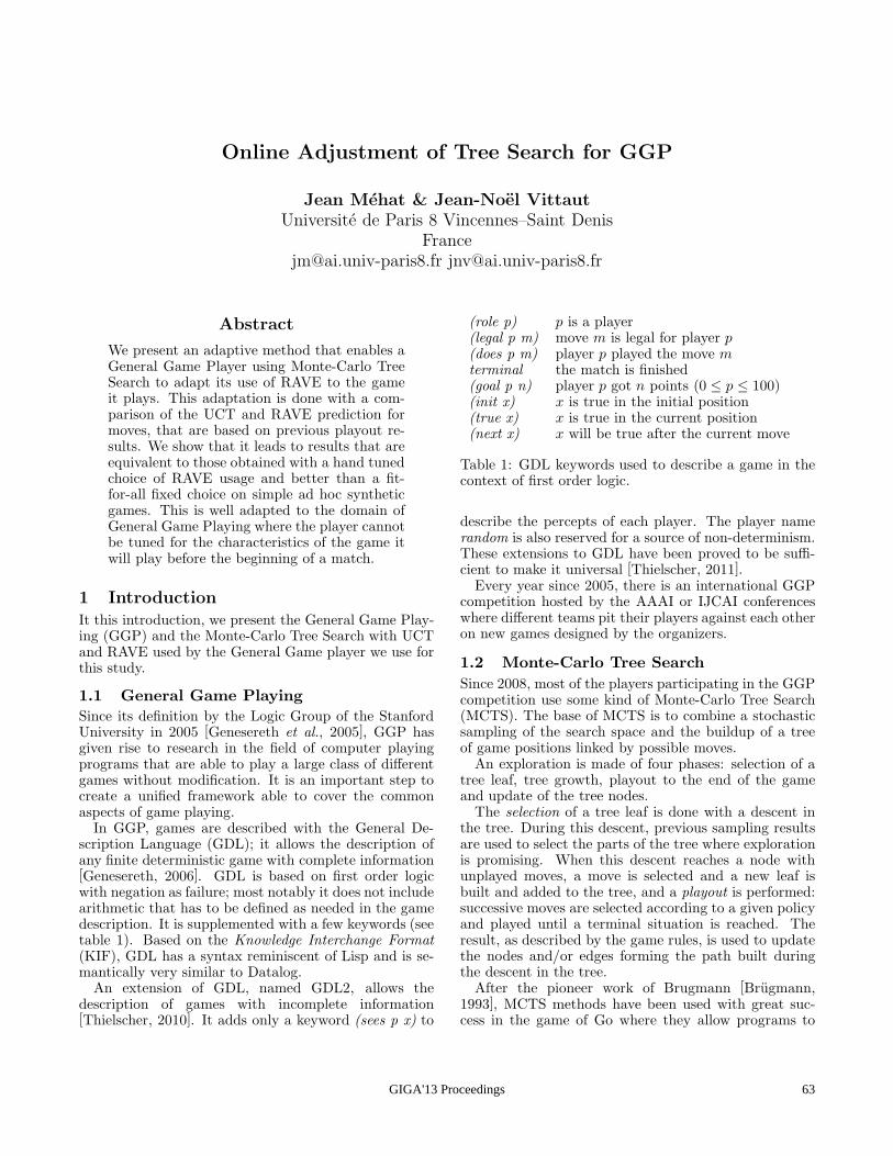
Online Adjustment of Tree Search for GGP
Jean Mehat & Jean-Noel Vittaut
Universite de Paris 8 Vincennes–Saint Denis
France
[email protected] [email protected]
Abstract
We present an adaptive method that enables aGeneral Game Player using Monte-Carlo TreeSearch to adapt its use of RAVE to the gameit plays. This adaptation is done with a com-parison of the UCT and RAVE prediction formoves, that are based on previous playout re-sults. We show that it leads to results that areequivalent to those obtained with a hand tunedchoice of RAVE usage and better than a fit-for-all fixed choice on simple ad hoc syntheticgames. This is well adapted to the domain ofGeneral Game Playing where the player cannotbe tuned for the characteristics of the game itwill play before the beginning of a match.
1 Introduction
It this introduction, we present the General Game Play-ing (GGP) and the Monte-Carlo Tree Search with UCTand RAVE used by the General Game player we use forthis study.
1.1 General Game Playing
Since its definition by the Logic Group of the StanfordUniversity in 2005 [Genesereth et al., 2005], GGP hasgiven rise to research in the field of computer playingprograms that are able to play a large class of differentgames without modification. It is an important step tocreate a unified framework able to cover the commonaspects of game playing.In GGP, games are described with the General De-
scription Language (GDL); it allows the description ofany finite deterministic game with complete information[Genesereth, 2006]. GDL is based on first order logicwith negation as failure; most notably it does not includearithmetic that has to be defined as needed in the gamedescription. It is supplemented with a few keywords (seetable 1). Based on the Knowledge Interchange Format(KIF), GDL has a syntax reminiscent of Lisp and is se-mantically very similar to Datalog.An extension of GDL, named GDL2, allows the
description of games with incomplete information[Thielscher, 2010]. It adds only a keyword (sees p x) to
(role p) p is a player(legal p m) move m is legal for player p(does p m) player p played the move mterminal the match is finished(goal p n) player p got n points (0 ≤ p ≤ 100)(init x) x is true in the initial position(true x) x is true in the current position(next x) x will be true after the current move
Table 1: GDL keywords used to describe a game in thecontext of first order logic.
describe the percepts of each player. The player namerandom is also reserved for a source of non-determinism.These extensions to GDL have been proved to be suffi-cient to make it universal [Thielscher, 2011].Every year since 2005, there is an international GGP
competition hosted by the AAAI or IJCAI conferenceswhere different teams pit their players against each otheron new games designed by the organizers.
1.2 Monte-Carlo Tree Search
Since 2008, most of the players participating in the GGPcompetition use some kind of Monte-Carlo Tree Search(MCTS). The base of MCTS is to combine a stochasticsampling of the search space and the buildup of a treeof game positions linked by possible moves.An exploration is made of four phases: selection of a
tree leaf, tree growth, playout to the end of the gameand update of the tree nodes.The selection of a tree leaf is done with a descent in
the tree. During this descent, previous sampling resultsare used to select the parts of the tree where explorationis promising. When this descent reaches a node withunplayed moves, a move is selected and a new leaf isbuilt and added to the tree, and a playout is performed:successive moves are selected according to a given policyand played until a terminal situation is reached. Theresult, as described by the game rules, is used to updatethe nodes and/or edges forming the path built duringthe descent in the tree.After the pioneer work of Brugmann [Brugmann,
1993], MCTS methods have been used with great suc-cess in the game of Go where they allow programs to
GIGA'13 Proceedings 63
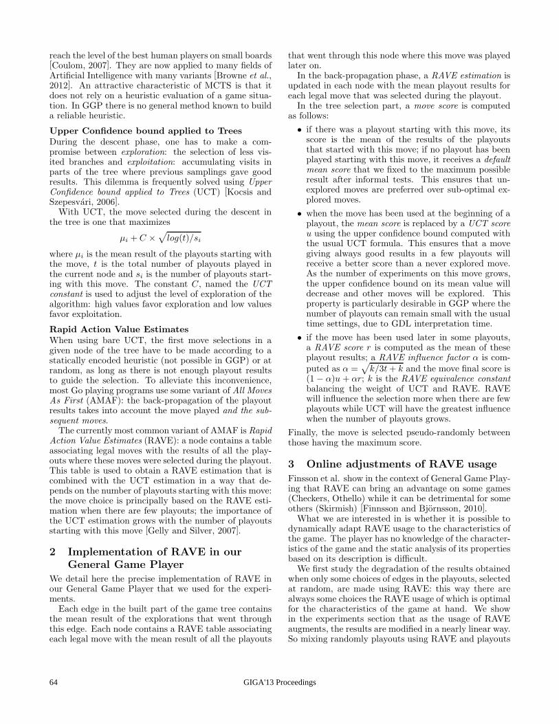
reach the level of the best human players on small boards[Coulom, 2007]. They are now applied to many fields ofArtificial Intelligence with many variants [Browne et al.,2012]. An attractive characteristic of MCTS is that itdoes not rely on a heuristic evaluation of a game situa-tion. In GGP there is no general method known to builda reliable heuristic.
Upper Confidence bound applied to Trees
During the descent phase, one has to make a com-promise between exploration: the selection of less vis-ited branches and exploitation: accumulating visits inparts of the tree where previous samplings gave goodresults. This dilemma is frequently solved using UpperConfidence bound applied to Trees (UCT) [Kocsis andSzepesvari, 2006].With UCT, the move selected during the descent in
the tree is one that maximizes
µi + C ×√log(t)/si
where µi is the mean result of the playouts starting withthe move, t is the total number of playouts played inthe current node and si is the number of playouts start-ing with this move. The constant C, named the UCTconstant is used to adjust the level of exploration of thealgorithm: high values favor exploration and low valuesfavor exploitation.
Rapid Action Value Estimates
When using bare UCT, the first move selections in agiven node of the tree have to be made according to astatically encoded heuristic (not possible in GGP) or atrandom, as long as there is not enough playout resultsto guide the selection. To alleviate this inconvenience,most Go playing programs use some variant of All MovesAs First (AMAF): the back-propagation of the playoutresults takes into account the move played and the sub-sequent moves.The currently most common variant of AMAF is Rapid
Action Value Estimates (RAVE): a node contains a tableassociating legal moves with the results of all the play-outs where these moves were selected during the playout.This table is used to obtain a RAVE estimation that iscombined with the UCT estimation in a way that de-pends on the number of playouts starting with this move:the move choice is principally based on the RAVE esti-mation when there are few playouts; the importance ofthe UCT estimation grows with the number of playoutsstarting with this move [Gelly and Silver, 2007].
2 Implementation of RAVE in our
General Game Player
We detail here the precise implementation of RAVE inour General Game Player that we used for the experi-ments.Each edge in the built part of the game tree contains
the mean result of the explorations that went throughthis edge. Each node contains a RAVE table associatingeach legal move with the mean result of all the playouts
that went through this node where this move was playedlater on.In the back-propagation phase, a RAVE estimation is
updated in each node with the mean playout results foreach legal move that was selected during the playout.In the tree selection part, a move score is computed
as follows:
• if there was a playout starting with this move, itsscore is the mean of the results of the playoutsthat started with this move; if no playout has beenplayed starting with this move, it receives a defaultmean score that we fixed to the maximum possibleresult after informal tests. This ensures that un-explored moves are preferred over sub-optimal ex-plored moves.
• when the move has been used at the beginning of aplayout, the mean score is replaced by a UCT scoreu using the upper confidence bound computed withthe usual UCT formula. This ensures that a movegiving always good results in a few playouts willreceive a better score than a never explored move.As the number of experiments on this move grows,the upper confidence bound on its mean value willdecrease and other moves will be explored. Thisproperty is particularly desirable in GGP where thenumber of playouts can remain small with the usualtime settings, due to GDL interpretation time.
• if the move has been used later in some playouts,a RAVE score r is computed as the mean of theseplayout results; a RAVE influence factor α is com-puted as α =
√k/3t+ k and the move final score is
(1 − α)u + αr; k is the RAVE equivalence constantbalancing the weight of UCT and RAVE. RAVEwill influence the selection more when there are fewplayouts while UCT will have the greatest influencewhen the number of playouts grows.
Finally, the move is selected pseudo-randomly betweenthose having the maximum score.
3 Online adjustments of RAVE usage
Finsson et al. show in the context of General Game Play-ing that RAVE can bring an advantage on some games(Checkers, Othello) while it can be detrimental for someothers (Skirmish) [Finnsson and Bjornsson, 2010].What we are interested in is whether it is possible to
dynamically adapt RAVE usage to the characteristics ofthe game. The player has no knowledge of the character-istics of the game and the static analysis of its propertiesbased on its description is difficult.We first study the degradation of the results obtained
when only some choices of edges in the playouts, selectedat random, are made using RAVE: this way there arealways some choices the RAVE usage of which is optimalfor the characteristics of the game at hand. We showin the experiments section that as the usage of RAVEaugments, the results are modified in a nearly linear way.So mixing randomly playouts using RAVE and playouts
GIGA'13 Proceedings64
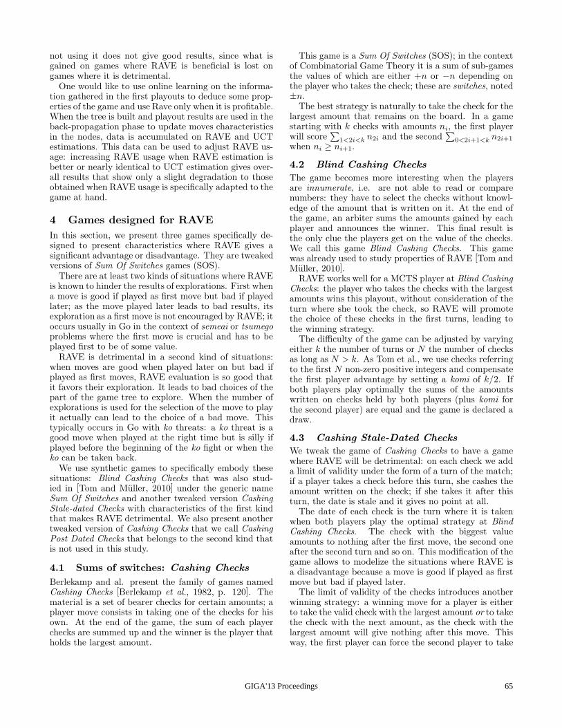
not using it does not give good results, since what isgained on games where RAVE is beneficial is lost ongames where it is detrimental.One would like to use online learning on the informa-
tion gathered in the first playouts to deduce some prop-erties of the game and use Rave only when it is profitable.When the tree is built and playout results are used in theback-propagation phase to update moves characteristicsin the nodes, data is accumulated on RAVE and UCTestimations. This data can be used to adjust RAVE us-age: increasing RAVE usage when RAVE estimation isbetter or nearly identical to UCT estimation gives over-all results that show only a slight degradation to thoseobtained when RAVE usage is specifically adapted to thegame at hand.
4 Games designed for RAVE
In this section, we present three games specifically de-signed to present characteristics where RAVE gives asignificant advantage or disadvantage. They are tweakedversions of Sum Of Switches games (SOS).There are at least two kinds of situations where RAVE
is known to hinder the results of explorations. First whena move is good if played as first move but bad if playedlater; as the move played later leads to bad results, itsexploration as a first move is not encouraged by RAVE; itoccurs usually in Go in the context of semeai or tsumegoproblems where the first move is crucial and has to beplayed first to be of some value.RAVE is detrimental in a second kind of situations:
when moves are good when played later on but bad ifplayed as first moves, RAVE evaluation is so good thatit favors their exploration. It leads to bad choices of thepart of the game tree to explore. When the number ofexplorations is used for the selection of the move to playit actually can lead to the choice of a bad move. Thistypically occurs in Go with ko threats: a ko threat is agood move when played at the right time but is silly ifplayed before the beginning of the ko fight or when theko can be taken back.We use synthetic games to specifically embody these
situations: Blind Cashing Checks that was also stud-ied in [Tom and Muller, 2010] under the generic nameSum Of Switches and another tweaked version CashingStale-dated Checks with characteristics of the first kindthat makes RAVE detrimental. We also present anothertweaked version of Cashing Checks that we call CashingPost Dated Checks that belongs to the second kind thatis not used in this study.
4.1 Sums of switches: Cashing Checks
Berlekamp and al. present the family of games namedCashing Checks [Berlekamp et al., 1982, p. 120]. Thematerial is a set of bearer checks for certain amounts; aplayer move consists in taking one of the checks for hisown. At the end of the game, the sum of each playerchecks are summed up and the winner is the player thatholds the largest amount.
This game is a Sum Of Switches (SOS); in the contextof Combinatorial Game Theory it is a sum of sub-gamesthe values of which are either +n or −n depending onthe player who takes the check; these are switches, noted±n.The best strategy is naturally to take the check for the
largest amount that remains on the board. In a gamestarting with k checks with amounts ni, the first playerwill score
∑1<2i<k
n2i and the second∑
0<2i+1<kn2i+1
when ni ≥ ni+1.
4.2 Blind Cashing Checks
The game becomes more interesting when the playersare innumerate, i.e. are not able to read or comparenumbers: they have to select the checks without knowl-edge of the amount that is written on it. At the end ofthe game, an arbiter sums the amounts gained by eachplayer and announces the winner. This final result isthe only clue the players get on the value of the checks.We call this game Blind Cashing Checks. This gamewas already used to study properties of RAVE [Tom andMuller, 2010].RAVE works well for a MCTS player at Blind Cashing
Checks: the player who takes the checks with the largestamounts wins this playout, without consideration of theturn where she took the check, so RAVE will promotethe choice of these checks in the first turns, leading tothe winning strategy.The difficulty of the game can be adjusted by varying
either k the number of turns or N the number of checksas long as N > k. As Tom et al., we use checks referringto the first N non-zero positive integers and compensatethe first player advantage by setting a komi of k/2. Ifboth players play optimally the sums of the amountswritten on checks held by both players (plus komi forthe second player) are equal and the game is declared adraw.
4.3 Cashing Stale-Dated Checks
We tweak the game of Cashing Checks to have a gamewhere RAVE will be detrimental: on each check we adda limit of validity under the form of a turn of the match;if a player takes a check before this turn, she cashes theamount written on the check; if she takes it after thisturn, the date is stale and it gives no point at all.The date of each check is the turn where it is taken
when both players play the optimal strategy at BlindCashing Checks. The check with the biggest valueamounts to nothing after the first move, the second oneafter the second turn and so on. This modification of thegame allows to modelize the situations where RAVE isa disadvantage because a move is good if played as firstmove but bad if played later.The limit of validity of the checks introduces another
winning strategy: a winning move for a player is eitherto take the valid check with the largest amount or to takethe check with the next amount, as the check with thelargest amount will give nothing after this move. Thisway, the first player can force the second player to take
GIGA'13 Proceedings 65
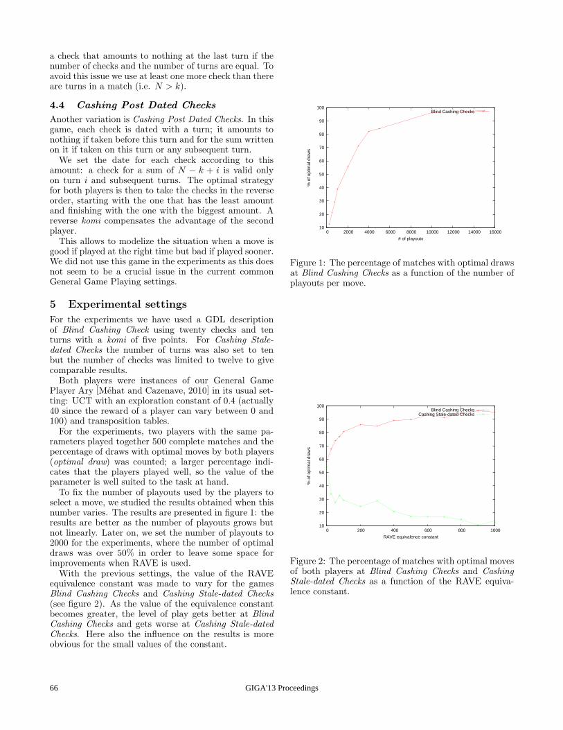
a check that amounts to nothing at the last turn if thenumber of checks and the number of turns are equal. Toavoid this issue we use at least one more check than thereare turns in a match (i.e. N > k).
4.4 Cashing Post Dated Checks
Another variation is Cashing Post Dated Checks. In thisgame, each check is dated with a turn; it amounts tonothing if taken before this turn and for the sum writtenon it if taken on this turn or any subsequent turn.We set the date for each check according to this
amount: a check for a sum of N − k + i is valid onlyon turn i and subsequent turns. The optimal strategyfor both players is then to take the checks in the reverseorder, starting with the one that has the least amountand finishing with the one with the biggest amount. Areverse komi compensates the advantage of the secondplayer.This allows to modelize the situation when a move is
good if played at the right time but bad if played sooner.We did not use this game in the experiments as this doesnot seem to be a crucial issue in the current commonGeneral Game Playing settings.
5 Experimental settings
For the experiments we have used a GDL descriptionof Blind Cashing Check using twenty checks and tenturns with a komi of five points. For Cashing Stale-dated Checks the number of turns was also set to tenbut the number of checks was limited to twelve to givecomparable results.Both players were instances of our General Game
Player Ary [Mehat and Cazenave, 2010] in its usual set-ting: UCT with an exploration constant of 0.4 (actually40 since the reward of a player can vary between 0 and100) and transposition tables.For the experiments, two players with the same pa-
rameters played together 500 complete matches and thepercentage of draws with optimal moves by both players(optimal draw) was counted; a larger percentage indi-cates that the players played well, so the value of theparameter is well suited to the task at hand.To fix the number of playouts used by the players to
select a move, we studied the results obtained when thisnumber varies. The results are presented in figure 1: theresults are better as the number of playouts grows butnot linearly. Later on, we set the number of playouts to2000 for the experiments, where the number of optimaldraws was over 50% in order to leave some space forimprovements when RAVE is used.With the previous settings, the value of the RAVE
equivalence constant was made to vary for the gamesBlind Cashing Checks and Cashing Stale-dated Checks(see figure 2). As the value of the equivalence constantbecomes greater, the level of play gets better at BlindCashing Checks and gets worse at Cashing Stale-datedChecks. Here also the influence on the results is moreobvious for the small values of the constant.
10
20
30
40
50
60
70
80
90
100
0 2000 4000 6000 8000 10000 12000 14000 16000
% o
f opt
imal
dra
ws
# of playouts
Blind Cashing Checks
Figure 1: The percentage of matches with optimal drawsat Blind Cashing Checks as a function of the number ofplayouts per move.
10
20
30
40
50
60
70
80
90
100
0 200 400 600 800 1000
% o
f opt
imal
dra
ws
RAVE equivalence constant
Blind Cashing ChecksCashing Stale-dated Checks
Figure 2: The percentage of matches with optimal movesof both players at Blind Cashing Checks and CashingStale-dated Checks as a function of the RAVE equiva-lence constant.
GIGA'13 Proceedings66
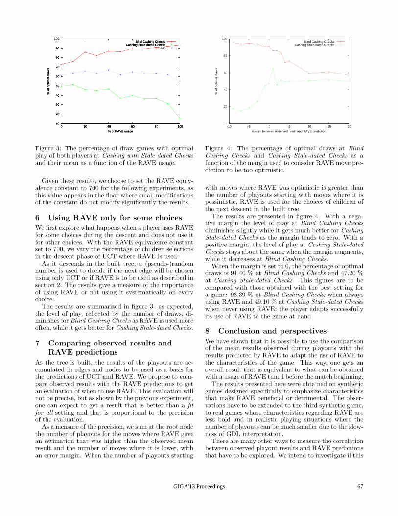
10
20
30
40
50
60
70
80
90
100
0 20 40 60 80 100
% o
f opt
imal
dra
ws
% of RAVE usage
Bind Cashing ChecksCashing Stale-dated Checks
10
20
30
40
50
60
70
80
90
100
0 20 40 60 80 100
% o
f opt
imal
dra
ws
% of RAVE usage
Bind Cashing ChecksCashing Stale-dated Checks
10
20
30
40
50
60
70
80
90
100
0 20 40 60 80 100
% o
f opt
imal
dra
ws
% of RAVE usage
Bind Cashing ChecksCashing Stale-dated Checks
mean
Figure 3: The percentage of draw games with optimalplay of both players at Cashing with Stale-dated Checksand their mean as a function of the RAVE usage.
Given these results, we choose to set the RAVE equiv-alence constant to 700 for the following experiments, asthis value appears in the floor where small modificationsof the constant do not modify significantly the results.
6 Using RAVE only for some choices
We first explore what happens when a player uses RAVEfor some choices during the descent and does not use itfor other choices. With the RAVE equivalence constantset to 700, we vary the percentage of children selectionsin the descent phase of UCT where RAVE is used.As it descends in the built tree, a (pseudo-)random
number is used to decide if the next edge will be chosenusing only UCT or if RAVE is to be used as described insection 2. The results give a measure of the importanceof using RAVE or not using it systematically on everychoice.The results are summarized in figure 3: as expected,
the level of play, reflected by the number of draws, di-minishes for Blind Cashing Checks as RAVE is used moreoften, while it gets better for Cashing Stale-dated Checks.
7 Comparing observed results and
RAVE predictions
As the tree is built, the results of the playouts are ac-cumulated in edges and nodes to be used as a basis forthe predictions of UCT and RAVE. We propose to com-pare observed results with the RAVE predictions to getan evaluation of when to use RAVE. This evaluation willnot be precise, but as shown by the previous experiment,one can expect to get a result that is better than a fitfor all setting and that is proportional to the precisionof the evaluation.As a measure of the precision, we sum at the root node
the number of playouts for the moves where RAVE gavean estimation that was higher than the observed meanresult and the number of moves where it is lower, withan error margin. When the number of playouts starting
0
20
40
60
80
100
-10 -5 0 5 10 15 20
% o
f opt
imal
dra
ws
margin between observed result and RAVE prediction
Blind Cashing ChecksCashing Stale-dated Checks
Figure 4: The percentage of optimal draws at BlindCashing Checks and Cashing Stale-dated Checks as afunction of the margin used to consider RAVE move pre-diction to be too optimistic.
with moves where RAVE was optimistic is greater thanthe number of playouts starting with moves where it ispessimistic, RAVE is used for the choices of children ofthe next descent in the built tree.The results are presented in figure 4. With a nega-
tive margin the level of play at Blind Cashing Checksdiminishes slightly while it gets much better for CashingStale-dated Checks as the margin tends to zero. With apositive margin, the level of play at Cashing Stale-datedChecks stays about the same when the margin augments,while it decreases at Blind Cashing Checks.When the margin is set to 0, the percentage of optimal
draws is 91.40 % at Blind Cashing Checks and 47.20 %at Cashing Stale-dated Checks. This figures are to becompared with those obtained with the best setting fora game: 93.39 % at Blind Cashing Checks when alwaysusing RAVE and 49.10 % at Cashing Stale-dated Checkswhen never using RAVE: the player adapts successfullyits use of RAVE to the game at hand.
8 Conclusion and perspectives
We have shown that it is possible to use the comparisonof the mean results observed during playouts with theresults predicted by RAVE to adapt the use of RAVE tothe characteristics of the game. This way, one gets anoverall result that is equivalent to what can be obtainedwith a usage of RAVE tuned before the match beginning.The results presented here were obtained on synthetic
games designed specifically to emphasize characteristicsthat make RAVE beneficial or detrimental. The obser-vations have to be extended to the third synthetic game,to real games whose characteristics regarding RAVE areless bold and in realistic playing situations where thenumber of playouts can be much smaller due to the slow-ness of GDL interpretation.There are many other ways to measure the correlation
between observed playout results and RAVE predictionsthat have to be explored. We intend to investigate if this
GIGA'13 Proceedings 67
correlation can be used to adapt the value of the RAVEequivalence constant.The method used here would not work in another syn-
thetic game built by summing the two games used, forexample alternating a move in Blind Cashing Checks anda move in Cashing Stale-dated Checks because the com-parison between observed results and RAVE predictionwas always calculated on the root node. It would bepossible to observe this correlation at every node whenit stores enough playout results.More generally, the method presented here uses infor-
mation that is already present in the tree built by theMCTS to determine characteristics of the game it plays.It could also be interesting outside of GGP for gameswhere characteristics regarding RAVE vary dependingon the position.
References
[Berlekamp et al., 1982] Elwyn R Berlekamp, John Hor-ton Conway, and Richard K Guy. Winning ways foryour mathematical plays. Volume 1. Academic Press,1982.
[Browne et al., 2012] Cameron B Browne, Edward Pow-ley, Daniel Whitehouse, Simon M Lucas, Peter I Cowl-ing, Philipp Rohlfshagen, Stephen Tavener, DiegoPerez, Spyridon Samothrakis, and Simon Colton. Asurvey of monte carlo tree search methods. Computa-tional Intelligence and AI in Games, IEEE Transac-tions on, 4(1):1–43, 2012.
[Brugmann, 1993] Bernd Brugmann. Monte carlo go,1993.
[Coulom, 2007] Remi Coulom. Efficient selectivity andbackup operators in monte-carlo tree search. In Com-puters and games, pages 72–83. Springer, 2007.
[Finnsson and Bjornsson, 2010] Hilmar Finnsson andYngvi Bjornsson. Learning simulation control in gen-eral game-playing agents. In Proc. 24th AAAI Conf.Artif. Intell., Atlanta, Georgia, pages 954–959, 2010.
[Gelly and Silver, 2007] Sylvain Gelly and David Silver.Combining online and offline knowledge in uct. In Pro-ceedings of the 24th international conference on Ma-chine learning, pages 273–280. ACM, 2007.
[Genesereth et al., 2005] Michael Genesereth, NathanielLove, and Barney Pell. General game playing:Overview of the aaai competition. AI magazine,26(2):62, 2005.
[Genesereth, 2006] Michael Genesereth. General gameplaying: Game description language specification,2006.
[Kocsis and Szepesvari, 2006] Levente Kocsis andCsaba Szepesvari. Bandit based monte-carlo plan-ning. Machine Learning: ECML 2006, pages 282–293,2006.
[Mehat and Cazenave, 2010] Jean Mehat and TristanCazenave. Ary, a general game playing program. In
13th board game studies colloquium, pages 168–170,2010.
[Thielscher, 2010] Michael Thielscher. A general gamedescription language for incomplete informationgames. In Proceedings of the Twenty-fourth NationalConference on Artificial Intelligence (AAAI 2010),pages 994–999, 2010.
[Thielscher, 2011] Michael Thielscher. The general gameplaying description language is universal. In Proceed-ings of the Twenty-Second international joint confer-ence on Artificial Intelligence-Volume Volume Two,pages 1107–1112. AAAI Press, 2011.
[Tom and Muller, 2010] David Tom and Martin Muller.A study of uct and its enhancements in an artificialgame. Advances in Computer Games, pages 55–64,2010.
GIGA'13 Proceedings68
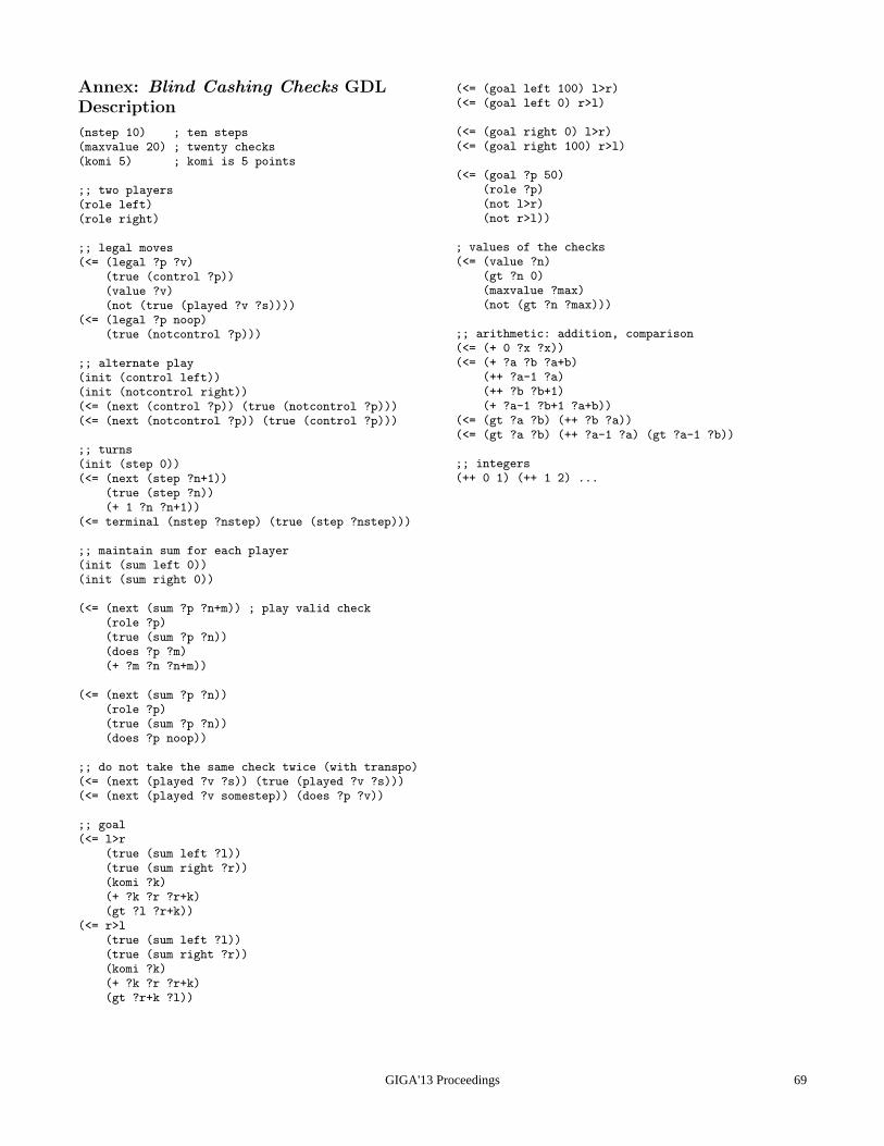
Annex: Blind Cashing Checks GDL
Description
(nstep 10) ; ten steps(maxvalue 20) ; twenty checks(komi 5) ; komi is 5 points
;; two players(role left)(role right)
;; legal moves(<= (legal ?p ?v)
(true (control ?p))(value ?v)(not (true (played ?v ?s))))
(<= (legal ?p noop)(true (notcontrol ?p)))
;; alternate play(init (control left))(init (notcontrol right))(<= (next (control ?p)) (true (notcontrol ?p)))(<= (next (notcontrol ?p)) (true (control ?p)))
;; turns(init (step 0))(<= (next (step ?n+1))
(true (step ?n))(+ 1 ?n ?n+1))
(<= terminal (nstep ?nstep) (true (step ?nstep)))
;; maintain sum for each player(init (sum left 0))(init (sum right 0))
(<= (next (sum ?p ?n+m)) ; play valid check(role ?p)(true (sum ?p ?n))(does ?p ?m)(+ ?m ?n ?n+m))
(<= (next (sum ?p ?n))(role ?p)(true (sum ?p ?n))(does ?p noop))
;; do not take the same check twice (with transpo)(<= (next (played ?v ?s)) (true (played ?v ?s)))(<= (next (played ?v somestep)) (does ?p ?v))
;; goal(<= l>r
(true (sum left ?l))(true (sum right ?r))(komi ?k)(+ ?k ?r ?r+k)(gt ?l ?r+k))
(<= r>l(true (sum left ?l))(true (sum right ?r))(komi ?k)(+ ?k ?r ?r+k)(gt ?r+k ?l))
(<= (goal left 100) l>r)(<= (goal left 0) r>l)
(<= (goal right 0) l>r)(<= (goal right 100) r>l)
(<= (goal ?p 50)(role ?p)(not l>r)(not r>l))
; values of the checks(<= (value ?n)
(gt ?n 0)(maxvalue ?max)(not (gt ?n ?max)))
;; arithmetic: addition, comparison(<= (+ 0 ?x ?x))(<= (+ ?a ?b ?a+b)
(++ ?a-1 ?a)(++ ?b ?b+1)(+ ?a-1 ?b+1 ?a+b))
(<= (gt ?a ?b) (++ ?b ?a))(<= (gt ?a ?b) (++ ?a-1 ?a) (gt ?a-1 ?b))
;; integers(++ 0 1) (++ 1 2) ...
GIGA'13 Proceedings 69

GIGA'13 Proceedings70
Stratified Logic Program Updates for General Game Playing
David [email protected]
University of AlbertaCanada
AbstractGeneral Game Playing Agents often play farmore poorly than their game-specific counter-parts due to the overhead of repeatedly query-ing an evolving logic program. A natural al-ternative approach is to instead maintain agrounded logic program and update it as thegame state changes. This paper presents asimple algorithm for updating a stratified logicprogram to reflect changes to the game stateand shows for Connect-4 that using logic pro-gram updates as opposed to recomputing fromscratch at each visited game-state constitutesa big-O improvement in the running time ofchecking for 4-in-a-row.
1 IntroductionGDL (Game Description Language1) is a minimalisticdeclarative language for describing games. Many gameshave large and complex descriptions in GDL. For thisreason, General Game Playing Agents often play farmore poorly than their game-specific counterparts dueto the overhead of constantly querying an evolving logicprogram. Although GDL requires that game descrip-tions be stratified, and there exist linear-time algorithmsfor querying stratified logic programs, the games areoften complex enough to make even linear algorithmsprohibitively slow. One natural alternative approach isto instead maintain a grounded logic program and up-date the program as the game state changes. This pa-per presents a simple algorithm for updating a stratifiedlogic program to reflect changes to the game state andshows for Connect-4 that using logic program updatesas opposed to recomputing from scratch at each visitedgame-state constitutes a big-O improvement in the run-ning time of checking for 4-in-a-row.Section 2 provides some definitions are provided for
talking about a grounded logic program. It is assumedthat the provided program is already grounded. The ap-proach described in this paper only applies to groundedprograms so a game whose grounding is too large to fit
1As defined in [Love et al., 2008]
in memory cannot be played using the techniques de-scribed in this paper. Section 3 defines the concept ofa numeric model of a logic program which is crucial tounderstanding the algorithm outlined in this paper. Sec-tion 4 provides the pseudocode for an approach to up-dating a stratified logic program and proves its correct-ness and running time. Section 5 shows, as an example,why this technique is expected to exhibit such impres-sive results for Connect 4. Section 6 describes some op-timizations that were used to speed up performance inan actual implementation of this technique. Section 7shows some experimental results for a couple commongames (including Connect 4).
2 Some DefinitionsStratified ProgramIn [Apt et al., 1988], a stratified logic program is definedas:
A program is stratified if there is a partitionP = P1∪ . . . ∪Pn
such that the following two conditions holdfor i = 1, . . . , n:1. If a relation symbol occurs positively [as a
positive literal] within a clause Pi, then itsdefinition is contained within
⋃j≤i
Pj
2. If a relation symbol occurs negatively [asa negative literal] within a clause Pi, thenits definition is contained within
⋃j<i
Pj
P1 can be emptyWe say that P is stratified by P1∪ . . . ∪Pn
and each Pi is called a stratum of PGiven a ruler = [h⇐= a1 . . . am ,¬b1 . . . bn]we can say h = h (r) to mean h is the head of rule r.b+ (r) = a1 . . . amandb− (r) = b1 . . . bndenote the sets of atoms contained in the body of r
as positive and negative literals respectively and theirunion is:
GIGA'13 Proceedings 71

b (r) = b+ (r)⋃b− (r)
If h = h (r), and b+ (r) ⊂ M and b− (r)⋂M = ∅,
then by r we know that h must be true and we can sayr supports h in M , writtenM (r) ` h
Dependency Graph[Apt et al., 1988] also defines the “dependency graph” ofa logic program P as:
The directed graph representing the relationrefers to between the relation symbols of P .Formally, p refers to q in P iff there is a clauseC in P where p is the relation symbol in thehead of C and q is the relation symbol of aliteral in the body of C.
Because this paper is only interested in grounded pro-grams, we will use dependency graph to mean the de-pendency graph between the atoms of a program as ifeach atom is its own relation symbol of arity 0.
Atom TypesIn a GDL program, the atoms can be divided into twoclasses. First, there are the true and does atoms here-after referred to as “base” atoms. These do not appearin the head of any rule and are instead determined bythe game state and players’ moves respectively. All theremaining atoms are “view” atoms. These atoms’ valuesare determined by a stratified logic program which de-scribes the game. This program must be solved in orderto ascertain a player’s legal moves, to tell whether thegame is in a terminal position, to compute child posi-tions, and to determine the winner of the game.
Game StateA game state S is a subset of the base atoms in a gameG which are taken to be “true” in this game state.For the purposes of this paper, a game state includes
assignments to does atoms as well as true.
Game State ProgramGiven a game description G as a set of rules and a gamestate S, we define the game state program PG (S) asG ∪ S (ie each atom a ∈ S is a fact in PG (S)).
Canonical StratificationIn Lemma 1 of [Apt et al., 1988], they show by construc-tion that a program is stratified if the dependency graphfor that program contains no negative edges as part of acycle.This is done by taking the strongly connected compo-
nents P1 . . . Pn of the dependency graph of P and order-ing them topologically. They then go on to show thatthis partitioning P1∪ . . . ∪Pn constitutes a stratificationof P .For a given game G, let G1 . . . Gn be the stratification
of G obtained in this way. We will refer to this as thecanonical stratification of G. Furthermore, given agame-state program PG (S) for any game-state S, it iseasy to see that P1 = S and P2 . . . Pn+1 = G1 . . . Gn
constitutes a stratification of PG (S) which we can callthe canonical stratification of PG (S).Because P2 . . . Pn+1 is always the same regardless of
the game state, we can assign to each rule r ∈ G a levell (r) = k|r ∈ Pk
In other words, the level of r is the stratum in whichr occurs in the canonical stratification of PG (S) for anystate S.In addition to giving each rule a level, it will also be
useful to assign a level to each atom.The level of any view atom a is the maximum level
over all rules which have a as their head:l (a) = max
a=h(r)l (r)
The level of any base atom is just 1l (b) = 1
Supported ModelA supported modelM of a game state program PG (S)is a set of atoms M such that S ⊂M and for each viewatom h ∈ G, there is a rule r that supports h in M . (ie∃rM (r) ` h)
Stable ModelA stable model orminimal model of S is a supportedmodel M that is minimal in the sense that no subset ofM is a supported model of S.As [Apt et al., 1988] show, the unique minimal model
MP of a program P stratified by P = P1∪ . . . ∪Pn isMP = Mn
whereM1 = TP1
↑ ω (∅)and∀k, Mk = TPk
↑ ω (Mk−1).Here TP is the immediate consequence operator mean-
ing for some set of facts M ,TP (M) = h|∃r ∈ P : M (r) ` hand TP ↑ ω is defined by• TP ↑ 0 (M) = M
• TP ↑ (n + 1) (M) = TP (TP ↑ n (M)) ∪ TP ↑ n (M)
• TP ↑ ω (M) =∞⋃
n=0
TP ↑ n (M)
Since P is finite and we’re only interested in groundedprograms, TP ↑ ω (M) can be obtained by repeatedlyadding all consequences of P ∪M to M until M con-verges.
3 An Ordering on Rules and Atoms3.1 Finding LevelsWe start by finding the level (as defined in the abovesection) of each rule and each atom.Since the level of any rule or atom does not depend on
the game state, this can be done in preprocessing. Wesimply build the dependency graph of G and then topo-logically sort the rules. Then we identify the stronglyconnect components and index them according to theorder of first appearance in the topologically sorted list.
GIGA'13 Proceedings72
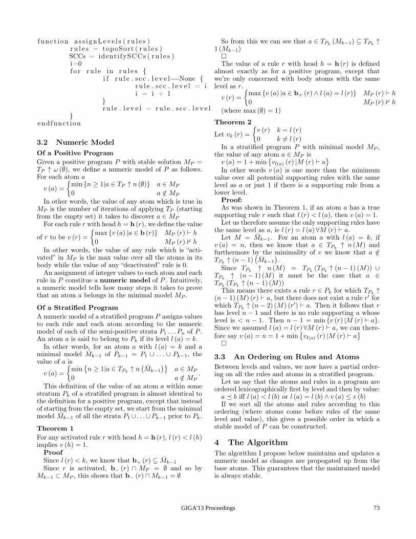
f unc t i on a s s i gnLev e l s ( r u l e s )r u l e s = topoSort ( r u l e s )SCCs = ident i fySCCs ( r u l e s )i=0f o r r u l e in r u l e s
i f r u l e . s c c . l e v e l==None ru l e . s c c . l e v e l = ii = i + 1
ru l e . l e v e l = ru l e . s c c . l e v e l
endfunct ion
3.2 Numeric ModelOf a Positive ProgramGiven a positive program P with stable solution MP =TP ↑ ω (∅), we define a numeric model of P as follows.For each atom a
v (a) =
min n ≥ 1|a ∈ TP ↑ n (∅) a ∈MP
0 a /∈MP
In other words, the value of any atom which is true inMP is the number of iterations of applying TP (startingfrom the empty set) it takes to discover a ∈MP
For each rule r with head h = h (r), we define the value
of r to be v (r) =
max v (a) |a ∈ b (r) MP (r) ` h
0 MP (r) 0 hIn other words, the value of any rule which is “acti-
vated” in MP is the max value over all the atoms in itsbody while the value of any “deactivated” rule is 0.An assignment of integer values to each atom and each
rule in P constitue a numeric model of P . Intuitively,a numeric model tells how many steps it takes to provethat an atom a belongs in the minimal model MP .
Of a Stratified ProgramA numeric model of a stratified program P assigns valuesto each rule and each atom according to the numericmodel of each of the semi-positive strata P1 . . . Pn of P .An atom a is said to belong to Pk if its level l (a) = k.In other words, for an atom a with l (a) = k and a
minimal model Mk−1 of Pk−1 = P1 ∪ . . . ∪ Pk−1, thevalue of a is
v (a) =
min
n ≥ 1|a ∈ TPk
↑ n(Mk−1
)a ∈MP
0 a /∈MP.
This definition of the value of an atom a within somestratum Pk of a stratified program is almost identical tothe definition for a positive program, except that insteadof starting from the empty set, we start from the minimalmodel Mk−1 of all the strata P1 ∪ . . .∪Pk−1 prior to Pk.
Theorem 1For any activated rule r with head h = h (r), l (r) < l (h)implies v (h) = 1.ProofSince l (r) < k, we know that b+ (r) ⊆ Mk−1Since r is activated, b− (r) ∩ MP = ∅ and so by
Mk−1 ⊂MP , this shows that b− (r) ∩Mk−1 = ∅
So from this we can see that a ∈ TPk(Mk−1) ⊆ TPk
↑1 (Mk−1)The value of a rule r with head h = h (r) is defined
almost exactly as for a positive program, except thatwe’re only concerned with body atoms with the samelevel as r.
v (r) =
max v (a) |a ∈ b+ (r) ∧ l (a) = l (r) MP (r) ` h
0 MP (r) 0 h
(where max (∅) = 1)
Theorem 2
Let vk (r) =
v (r) k = l (r)
0 k 6= l (r)In a stratified program P with minimal model MP ,
the value of any atom a ∈MP isv (a) = 1 + min
vl(a) (r) |M (r) ` a
In other words v (a) is one more than the minimum
value over all potential supporting rules with the samelevel as a or just 1 if there is a supporting rule from alower level.Proof:As was shown in Theorem 1, if an atom a has a true
supporting rule r such that l (r) < l (a), then v (a) = 1.Let us therefore assume the only supporting rules have
the same level as a, ie l (r) = l (a)∀M (r) ` a.Let M = Mk−1. For an atom a with l (a) = k, if
v (a) = n, then we know that a ∈ TPk↑ n (M) and
furthermore by the minimality of v we know that a /∈TPk↑ (n− 1)
(Mk−1
).
Since TPk↑ n (M) = TPk
(TPk↑ (n− 1) (M)) ∪
TPk↑ (n− 1) (M) it must be the case that a ∈
TPk(TPk
↑ (n− 1) (M))This means there exists a rule r ∈ Pk for which TPk
↑(n− 1) (M) (r) ` a, but there does not exist a rule r′ forwhich TPk
↑ (n− 2) (M) (r′) ` a. Then it follows that rhas level n − 1 and there is no rule supporting a whoselevel is < n − 1. Then n − 1 = min v (r) |M (r) ` a.Since we assumed l (a) = l (r)∀M (r) ` a, we can there-fore say v (a) = n = 1 + min
vl(a) (r) |M (r) ` a
3.3 An Ordering on Rules and AtomsBetween levels and values, we now have a partial order-ing on all the rules and atoms in a stratified program.Let us say that the atoms and rules in a program are
ordered lexicographically first by level and then by value:a b iff l (a) < l (b) or l (a) = l (b) ∧ v (a) ≤ v (b)If we sort all the atoms and rules according to this
ordering (where atoms come before rules of the samelevel and value), this gives a possible order in which astable model of P can be constructed.
4 The AlgorithmThe algorithm I propose below maintains and updates anumeric model as changes are propogated up from thebase atoms. This guarantees that the maintained modelis always stable.
GIGA'13 Proceedings 73
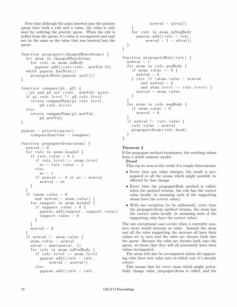
Note that although the pairs inserted into the priorityqueue have both a rule and a value, the value is onlyused for ordering the priority queue. When the rule ispolled from the queue, it’s value is recomputed and maynot be the same as the value that was inserted into thequeue.
f unc t i on propogate ( changedBaseAtoms ) f o r atom in changedBaseAtoms
f o r r u l e in atom . inBodypqueue . add ( ( r u l e=ru le , newVal=0))
whi l e pqueue . hasNext ( )propogateRule ( pqueue . p o l l ( ) )
func t i on compare (p1 , p2 ) //p1 and p2 are ( ru le , newVal ) pa i r si f p1 . r u l e . l e v e l != p2 . r u l e . l e v e l
r e turn compareNum(p1 . r u l e . l e v e l ,p2 . r u l e . l e v e l )
e l s ere turn compareNum(p1 . newVal ,
p2 . newVal )
pqueue = pr i o r i t yqueue (comparefunct ion = compare )
func t i on propogateAtom (atom) newval = 0f o r r u l e in atom . headof
i f r u l e . va lue > 0 i f r u l e . l e v e l == atom . l e v e l
nv = ru l e . va lue + 1e l s e
nv = 1i f newval == 0 or nv < newval
newval = nv
i f ( atom . value > 0
and newval > atom . value ) f o r support in atom . headof
i f support . va lue > 0 pqueue . add ( support , support . va lue )support . va lue = 0
newval = 0
i f newval != atom . value
atom . value = newvalnbval = min ( newval , 1)f o r r u l e in atom . inPosBody
i f r u l e . l e v e l == atom . l e v e lpqueue . add ( ( r u l e = ru le ,
newval = newval ) )e l s e
pqueue . add ( ( r u l e = ru le ,
newval = nbval ) )f o r r u l e in atom . inNegBody
pqueue . add ( ( r u l e = ru le ,newval = 1 − nbval ) )
func t i on propogateRule ( r u l e ) newval = 1f o r atom in ru l e . posBody
i f atom . value == 0 newval = 0
e l s e i f ( atom . value > newvaland newval > 0and atom . l e v e l == ru l e . l e v e l )
newval = atom . value
f o r atom in ru l e . negBody
i f atom . value > 0newval = 0
i f newval != ru l e . va lue
ru l e . va lue = newvalpropogateAtom ( ru l e . head )
Theorem 3If the propogate method terminates, the resulting valuesform a stable numeric model:ProofThis can be seen as the result of a couple observations:• Every time any value changes, the result is pro-
pogated to all the atoms which might possibly beaffected by that change.• Every time the propogateRule method is called,
when the method returns, the rule has the correctvalue locally (ie assuming each of the supportingatoms have the correct value).• With one exception (to be addressed), every time
the propogateAtom method returns, the atom hasthe correct value locally (ie assuming each of thesupporting rules have the correct value).
The one exceptional case occurs when a currently non-zero atom would increase in value. Instead the atomand all the rules supporting the increase all have theirvalues set to zero and the rules are thrown back intothe queue. Because the rules are thrown back onto thequeue, we know that they will all necessarily have theirvalues recomputed.The atom will also be recomputed unless all support-
ing rules have new value zero in which case it’s alreadycorrect.This means that for every atom which might poten-
tially change value, propogateAtom is called, and the
GIGA'13 Proceedings74
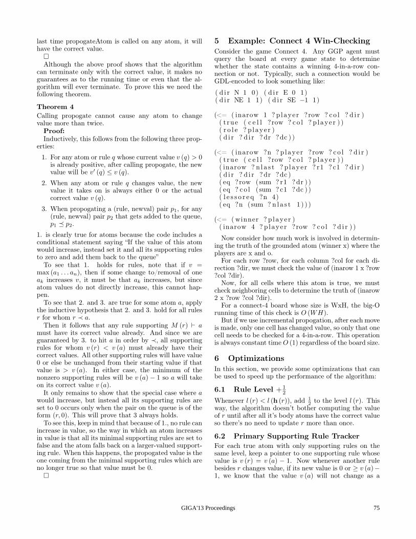
last time propogateAtom is called on any atom, it willhave the correct value.Although the above proof shows that the algorithm
can terminate only with the correct value, it makes noguarantees as to the running time or even that the al-gorithm will ever terminate. To prove this we need thefollowing theorem.
Theorem 4Calling propogate cannot cause any atom to changevalue more than twice.Proof:Inductively, this follows from the following three prop-
erties:
1. For any atom or rule q whose current value v (q) > 0is already positive, after calling propogate, the newvalue will be v′ (q) ≤ v (q).
2. When any atom or rule q changes value, the newvalue it takes on is always either 0 or the actualcorrect value v (q).
3. When propogating a (rule, newval) pair p1, for any(rule, newval) pair p2 that gets added to the queue,p1 p2.
1. is clearly true for atoms because the code includes aconditional statement saying “If the value of this atomwould increase, instead set it and all its supporting rulesto zero and add them back to the queue”To see that 1. holds for rules, note that if v =
max (a1 . . . an), then if some change to/removal of oneak increases v, it must be that ak increases, but sinceatom values do not directly increase, this cannot hap-pen.To see that 2. and 3. are true for some atom a, apply
the inductive hypothesis that 2. and 3. hold for all rulesr for whom r ≺ a.Then it follows that any rule supporting M (r) ` a
must have its correct value already. And since we areguaranteed by 3. to hit a in order by ≺, all supportingrules for whom v (r) < v (a) must already have theircorrect values. All other supporting rules will have value0 or else be unchanged from their starting value if thatvalue is > v (a). In either case, the minimum of thenonzero supporting rules will be v (a)− 1 so a will takeon its correct value v (a).It only remains to show that the special case where a
would increase, but instead all its supporting rules areset to 0 occurs only when the pair on the queue is of theform (r, 0). This will prove that 3 always holds.To see this, keep in mind that because of 1., no rule can
increase in value, so the way in which an atom increasesin value is that all its minimal supporting rules are set tofalse and the atom falls back on a larger-valued support-ing rule. When this happens, the propogated value is theone coming from the minimal supporting rules which areno longer true so that value must be 0.
5 Example: Connect 4 Win-CheckingConsider the game Connect 4. Any GGP agent mustquery the board at every game state to determinewhether the state contains a winning 4-in-a-row con-nection or not. Typically, such a connection would beGDL-encoded to look something like:
( d i r N 1 0) ( d i r E 0 1)( d i r NE 1 1) ( d i r SE −1 1)
(<= ( inarow 1 ? p laye r ?row ? co l ? d i r )( t rue ( c e l l ?row ? co l ? p laye r ) )( r o l e ? p laye r )( d i r ? d i r ? dr ?dc ) )
(<= ( inarow ?n ? p laye r ?row ? co l ? d i r )( t rue ( c e l l ?row ? co l ? p laye r ) )( inarow ? n l a s t ? p laye r ? r1 ? c1 ? d i r )( d i r ? d i r ? dr ?dc )( eq ?row (sum ? r1 ?dr ) )( eq ? c o l (sum ?c1 ?dc ) )( l e s s o r e q ?n 4)( eq ?n (sum ? n l a s t 1 ) ) )
(<= ( winner ? p laye r )( inarow 4 ? p laye r ?row ? co l ? d i r ) )
Now consider how much work is involved in determin-ing the truth of the grounded atom (winner x) where theplayers are x and o.For each row ?row, for each column ?col for each di-
rection ?dir, we must check the value of (inarow 1 x ?row?col ?dir).Now, for all cells where this atom is true, we must
check neighboring cells to determine the truth of (inarow2 x ?row ?col ?dir).For a connect-4 board whose size is WxH, the big-O
running time of this check is O (WH).But if we use incremental propogation, after each move
is made, only one cell has changed value, so only that onecell needs to be checked for a 4-in-a-row. This operationis always constant time O (1) regardless of the board size.
6 OptimizationsIn this section, we provide some optimizations that canbe used to speed up the performance of the algorithm:
6.1 Rule Level +12
Whenever l (r) < l (h (r)), add 12 to the level l (r). This
way, the algorithm doesn’t bother computing the valueof r until after all it’s body atoms have the correct valueso there’s no need to update r more than once.
6.2 Primary Supporting Rule TrackerFor each true atom with only supporting rules on thesame level, keep a pointer to one supporting rule whosevalue is v (r) = v (a) − 1. Now whenever another rulebesides r changes value, if its new value is 0 or ≥ v (a)−1, we know that the value v (a) will not change as a
GIGA'13 Proceedings 75
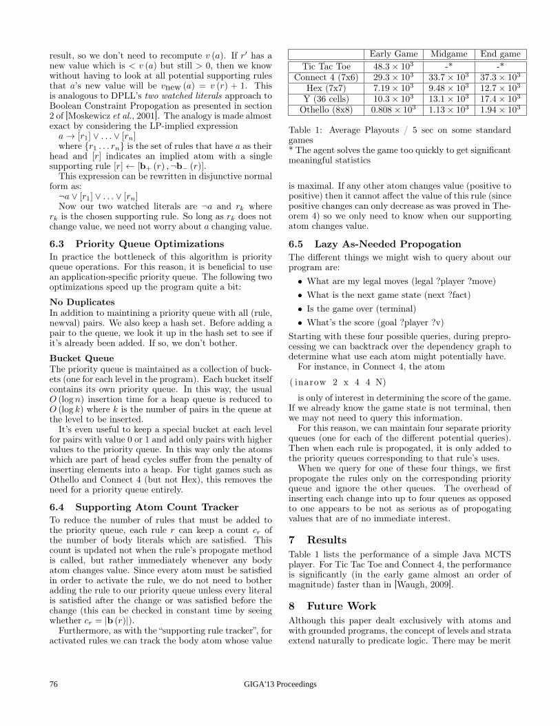
result, so we don’t need to recompute v (a). If r′ has anew value which is < v (a) but still > 0, then we knowwithout having to look at all potential supporting rulesthat a’s new value will be vnew (a) = v (r) + 1. Thisis analogous to DPLL’s two watched literals approach toBoolean Constraint Propogation as presented in section2 of [Moskewicz et al., 2001]. The analogy is made almostexact by considering the LP-implied expressiona→ [r1] ∨ . . . ∨ [rn]where r1 . . . rn is the set of rules that have a as their
head and [r] indicates an implied atom with a singlesupporting rule [r]← [b+ (r) ,¬b− (r)].This expression can be rewritten in disjunctive normal
form as:¬a ∨ [r1] ∨ . . . ∨ [rn]Now our two watched literals are ¬a and rk where
rk is the chosen supporting rule. So long as rk does notchange value, we need not worry about a changing value.
6.3 Priority Queue OptimizationsIn practice the bottleneck of this algorithm is priorityqueue operations. For this reason, it is beneficial to usean application-specific priority queue. The following twooptimizations speed up the program quite a bit:
No DuplicatesIn addition to maintining a priority queue with all (rule,newval) pairs. We also keep a hash set. Before adding apair to the queue, we look it up in the hash set to see ifit’s already been added. If so, we don’t bother.
Bucket QueueThe priority queue is maintained as a collection of buck-ets (one for each level in the program). Each bucket itselfcontains its own priority queue. In this way, the usualO (log n) insertion time for a heap queue is reduced toO (log k) where k is the number of pairs in the queue atthe level to be inserted.It’s even useful to keep a special bucket at each level
for pairs with value 0 or 1 and add only pairs with highervalues to the priority queue. In this way only the atomswhich are part of head cycles suffer from the penalty ofinserting elements into a heap. For tight games such asOthello and Connect 4 (but not Hex), this removes theneed for a priority queue entirely.
6.4 Supporting Atom Count TrackerTo reduce the number of rules that must be added tothe priority queue, each rule r can keep a count cr ofthe number of body literals which are satisfied. Thiscount is updated not when the rule’s propogate methodis called, but rather immediately whenever any bodyatom changes value. Since every atom must be satisfiedin order to activate the rule, we do not need to botheradding the rule to our priority queue unless every literalis satisfied after the change or was satisfied before thechange (this can be checked in constant time by seeingwhether cr = |b (r)|).Furthermore, as with the “supporting rule tracker”, for
activated rules we can track the body atom whose value
Early Game Midgame End gameTic Tac Toe 48.3× 10³ -* -*
Connect 4 (7x6) 29.3× 10³ 33.7× 10³ 37.3× 103
Hex (7x7) 7.19× 10³ 9.48× 10³ 12.7× 10³
Y (36 cells) 10.3× 10³ 13.1× 10³ 17.4× 10³
Othello (8x8) 0.808× 10³ 1.13× 10³ 1.94× 10³
Table 1: Average Playouts / 5 sec on some standardgames* The agent solves the game too quickly to get significantmeaningful statistics
is maximal. If any other atom changes value (positive topositive) then it cannot affect the value of this rule (sincepositive changes can only decrease as was proved in The-orem 4) so we only need to know when our supportingatom changes value.
6.5 Lazy As-Needed PropogationThe different things we might wish to query about ourprogram are:• What are my legal moves (legal ?player ?move)• What is the next game state (next ?fact)• Is the game over (terminal)• What’s the score (goal ?player ?v)
Starting with these four possible queries, during prepro-cessing we can backtrack over the dependency graph todetermine what use each atom might potentially have.For instance, in Connect 4, the atom
( inarow 2 x 4 4 N)
is only of interest in determining the score of the game.If we already know the game state is not terminal, thenwe may not need to query this information.For this reason, we can maintain four separate priority
queues (one for each of the different potential queries).Then when each rule is propogated, it is only added tothe priority queues corresponding to that rule’s uses.When we query for one of these four things, we first
propogate the rules only on the corresponding priorityqueue and ignore the other queues. The overhead ofinserting each change into up to four queues as opposedto one appears to be not as serious as of propogatingvalues that are of no immediate interest.
7 ResultsTable 1 lists the performance of a simple Java MCTSplayer. For Tic Tac Toe and Connect 4, the performanceis significantly (in the early game almost an order ofmagnitude) faster than in [Waugh, 2009].
8 Future WorkAlthough this paper dealt exclusively with atoms andwith grounded programs, the concept of levels and strataextend naturally to predicate logic. There may be merit
GIGA'13 Proceedings76
in finding ways to construct the true atoms and findtheir values on the fly and assign levels based on thecorresponding predicate to each atom. This could beparticularly useful for programs where a predicate hasa large arity, but only a small subset of the groundedinstances of that predicate are ever true simultaneously.It would be interesting to optimize this approach us-ing generated C++ code as in [Waugh, 2009]. Addi-tionally, it would be useful to have an upper bound onthe ratio # atom values changed in numeric model
# atom values changed in stable model . Ofcourse for tight programs, this is just 1, but many games,such as Hex, Y, and Go, require loopy programs. In thesecases it would be interesting to know exactly how much“extra” work is necessary to maintain that information.Perhaps propogation would run in faster amortized timeif we loosen the restriction on values which atoms andrules can take on to say v (a) is greater than the value ofsome supporting rule and v (r) is greater than or equalto the value of all same-level supporting atoms.
9 ConclusionBy recognizing which aspects of the game change withrespect to each move, we can eliminate much of the re-peated work done for querying game states. Incorporat-ing techniques from logic program updates is a promis-ing path for closing the performance gap between gen-eral game playing agents and their game-specific coun-terparts.
AcknowledgmentsThank you to the University of Alberta GAMES Group.Also special thanks to Jia You and Ryan Hayward forall their help with this work.
References[Apt et al., 1988] Krzysztof R Apt, Howard A Blair, and
AdrianWalker. Towards a theory of declarative knowl-edge. Foundations of deductive databases and logicprogramming, pages 89–148, 1988.
[Love et al., 2008] Nathaniel Love, Timothy Hinrichs,David Haley, Eric Schkufza, and Michael Genesereth.General game playing: Game description languagespecification, 2008.
[Moskewicz et al., 2001] Matthew W Moskewicz,Conor F Madigan, Ying Zhao, Lintao Zhang, andSharad Malik. Chaff: Engineering an efficient satsolver. In Proceedings of the 38th annual DesignAutomation Conference, pages 530–535. ACM, 2001.
[Waugh, 2009] Kevin Waugh. Faster state manipulationin general games using generated code. Proceedingsof the 1st general intelligence in game-playing agents(GIGA), 2009.
GIGA'13 Proceedings 77


