The Illusion of Control, Cognitive Dissonance and Farmer Perception of

GM Crops

David R. Just Assistant Professor

Applied Economics and Management Cornell University 254 Warren Hall Ithaca, NY 14853 (607) 255-2086

drj3@cornell.edu

Michael J. Roberts* Economic Research Service

U.S. Department of Agriculture

Paper prepared for presentation at the Annual Meeting of the AAEA, Denver, Colorado, August 1-4, 2004.

Abstract We examine the correlation between farmers’ beliefs and practices regarding GM crops with yield shocks from the previous year the crop was grown. Farmers who may have had poor yields due to weather, were more likely to change adoption decisions. Yields marginally affect farmers’ beliefs regarding the EU ban on GMO’s, or the adverse environmental affects of GM crops. This behavior is consistent with many known psychological biases.

*Views expressed are those of the authors and not necessarily those of the U.S. Department of Agriculture.

1

The Illusion of Control, Cognitive Dissonance and Farmer Perception of

GM Crops

“It must be indicative of something, besides the redistribution of wealth. List of possible

explanations. One: I'm willing it. Inside where nothing shows, I'm the essence of a man

spinning double-headed coins, and betting against himself in private atonement for an

unremembered past.” – Guildenstern in Rosencrantz and Guildenstern are Dead, by Tom

Stoppard after 89 consecutive coin tosses resulting in heads.

The adoption of new technologies has been most often modeled as a function of some

combination of profitability, risk preferences, information and human capital constraints.

When new technologies become available, there is often little or even conflicting

information on the explicit trade-offs involved in adoption. This was the case in the late

1990s and early 2000s, as farmers began considering the use of genetically modified (GM)

crops for the purpose of pest damage control. Although Bt corn and cotton were touted for

increases in average yield and lower pest control costs, this information was coupled with

news of consumer fears, and warnings that the European Union and others would not

import GM crops. Further, concerns over environmental externalities were highly

publicized.

Amid conflicting information, it is easy to understand why farmers might take on

different adoption strategies. Fernandez-Cornejo finds that few variables besides location

have strong predictive power in explaining the use of Bt corn by US farmers in this time

period. Geographic patterns of adoption behavior also appear somewhat idiosyncratic. In

an atmosphere of confusion and ill-defined incentives, it seems only natural that less

2

rational decision-making may be prevalent. In this paper, we explore the evidence that

farmers were unable to mentally separate the affects of general adverse weather conditions

and the specific use of GM vs. non-GM crops on yields. Further, we examine the

phenomenon of cognitive dissonance in deciding to adopt or dis-adopt GM crops. After

taking account of various factors in production, and the probability of having previously

adopted, we find negative yield shocks experienced in a county in previous years cause

subsequent adoption of Bt cotton and perhaps corn. This finding may indicate false

attribution due to hindsight biases and the illusion of control, as individuals assume their

poor performance was somehow due to poor choices rather than uncontrollable events

(these yield shocks appear weather related and show no autocorrelation). In addition, we

find some evidence supporting the notion that previous years’ yield shocks are correlated

with the perception of environmental and export problems with Bt crops. This may suggest

cognitive dissonance, or seeking to rationalize one’s choices by altering beliefs regarding

the relative sizes of benefits and costs.

In the following section we briefly outline the literature regarding technology

adoption as it relates to Bt corn and cotton in the US. We also describe the experimental

literature detailing the effects of hindsight bias, the illusion of control, and cognitive

dissonance. We then describe the data to be used in estimation and our methods. In the

following section we present results and discussion regarding the use of Bt corn and

cotton.

3

Rational versus Irrational Adoption

From its inception, the economic literature has acknowledged the large role played by

information in technology adoption. Rogers defined adoption as a mental process

beginning when an individual first hears of a technology, which eventually leads to use of

the technology. Schultz describes periods of disequilibrium that may exist when market

players are beginning to understand a new technology. During this period of

disequilibrium, a lack of information on newer technologies leads to experimentation, and

eventually to a new equilibrium. Although many acknowledge that a lack of information

leads to inefficiencies, the literature has focused mainly on inefficiencies due to

uninformed but rational actions. In their review of the technology adoption literature,

Feder, Just and Zilberman note that adoption is almost exclusively modeled as the result of

expected utility of profit maximization. O’Mara modeled the information gathering of

farmers as a Bayesian process, whereby they use the information from their own and

neighbor’s yields to update their prior beliefs about the technology. O’Mara’s work has

inspired many similar studies examining the spread of information regarding new

technologies and the influence on adoption.

More specifically, the adoption of Bt corn and cotton in the US has been

widespread and well publicized. USDA has found significant variability in adoption across

states. Fernandez-Cornejo and McBride specifically examine the effects of producer

attributes on the adoption of Bt corn and cotton, as well as several other GM crops.

Although few attributes were statistically significant, education and farm size appear to

positively affect the adoption of Bt corn. Growth of adoption of a new technology

(diffusion) is usually continuous for such a new technology; in this case, however,

adoption rates dipped slightly in the early 2000s. In 1999 the European Union (EU) began

4

a moratorium on the import of nearly all genetically modified corn varieties. This ban on

GM corn led to a marked decline in US corn exports to the EU. Prior to the ban, the US

had averaged nearly $300 million in corn exports to EU, compared to $70 million annually

for the previous three years. Following the EU ban on GM crops, the percent of US corn

farmers using Bt fell from near 30% to less than 20%. Alexander, Fernandez-Cornejo and

Goodhue use focus group responses from 1999 and 2000 to analyze farmer opinions and

information regarding the use of GM crops. They find that many farmers worry about the

possibilities of marketing genetically modified crops given the consumer furor in the EU

and rising consumer issues in the US. There are wide differences in opinions on whether

the higher average yields and lower pesticide costs are worth the added expense.

Interestingly, some farmers view Bt varieties as a form of insurance. Their responses

appear to reflect a lack of clear information, as in the disequilibrium Schultz suggests.

Psychology and Expectations

In the opening act of Rosencrantz and Guildestern are Dead (Stoppard)

Guildenstern repeatedly flips a coin, resulting each time in a draw of heads. Guildenstern

begins to believe the singular occurrence must be the result of fate, or his own

subconscious will. Psychologists and behavioral economists have consistently found

humans to be poor processors of information. When presented with new information, there

are several systematic and known biases that shape the use of this information for decision-

making. In the case of Bt corn and cotton, with very little information regarding future

profitability, psychological biases may have become more influential in farmer adoption

decisions.

Particularly notable biases are those that arise when individuals try to infer

causation from seemingly correlated events. In an early study on the psychology of

5

correlation and causation, Kahneman and Tversky found an illusion of causation associated

with reversion to a mean. In his study of Israeli flight trainers, Kahneman and Tversky

tried to assess the effectiveness of rewards (punishments) given after particularly good

(bad) flights. It was the common view among flight trainers that punishments were more

effective than rewards because pilots did better on average after receiving punishment, but

worse on average after receiving rewards. Kahneman and Tversky found no correlation

between the punishments/rewards and pilot performance. Rather, the pattern of behavior

was observed because punishments (rewards) were only given after exceptionally bad

(good) performance. The probability of exceptional performances is smaller than that of an

average performance. Hence random outcomes had been misinterpreted as the effect of

trainer actions. Subsequent studies delineated this phenomenon into two separate

behavioral biases: illusion of correlation, and illusion of control.

Illusion of correlation occurs when individuals perceive uncorrelated events to be

correlated. Gilovich, Vallone and Tversky found this to be common among basketball fans

(and subsequent studies have found it among bettors). In what they called the hot hand

bias, individuals perceive basketball shots to be correlated over time, with players going on

streaks. However, statistical analysis of shooting data provides little evidence of positive

autocorrelation in shooting accuracy. (Although, there appears to be slight negative

autocorrelation.) Similar phenomena have been observed in many other settings. In

general, individuals expect a series of uncorrelated draws (like the flipping of a unbiased

coin) to alternate, which would actually be consistent with negative correlation. When data

reflect the length of streaks that are natural in an uncorrelated series, people mistake the

streaks for evidence of correlation. In general, individuals appear to read too much into

happenstance occurrences, trying to find deterministic explanations for random events.

6

Tversky and Kahneman call this belief in the law of small numbers, or, an irrational belief

that small samples must reflect properties of the larger population. Grether explored this

phenomenon using economic experiments and found that individuals place too much

emphasis on the most recent information when making economic decisions, a form of

representativeness bias.

Illusion of control occurs when individuals misinterpret the degree of control they

have over situations and outcomes. For example, it has been observed that individuals

throw dice harder when desiring larger numbers, but softer when desiring smaller numbers

(Henslin). Langer found evidence of the illusion of control by allowing subjects to bet on

the outcome of dice rolls. Some subjects were permitted to bet on the outcome before the

roll of the dice and others bet after the dice were rolled, but before the outcome was

revealed. Those betting before the roll made larger bets than those betting after the roll. It

is theorized that those who bet more believed they had a greater influence on the outcome

because the roll had not yet taken place. The illusion of control appears to be linked with

several attributes of the random situation. Langer cites several of these cues that, when

trivially linked to random outcomes, lead to an illusion of control:

• Competition – payoffs are dependent on others’ outcomes

• Choice – the random process is preceded by some (possibly trivial) choice

• Active involvement – participation in generating the random outcome

• Response familiarity – familiarity with the types of outcomes

As illusion of correlation and illusion of control combined to blur the effects of flight

trainers, control and correlation may also be misinterpreted by farmers making technology

adoption decisions. Farmers face uncertainty on many levels. Some of this uncertainty is

correlated across geographic areas, while some shocks are farm specific. By examining the

7

effects of local and transitory regional supply shocks on subsequent individual decisions,

we detect adoption patterns that may be attributable to illusions of correlation and control.

Cognitive Dissonance

Another well-documented psychological phenomenon is cognitive dissonance.

Once having made an irreversible decision, such as this year’s planting, individuals are

often faced with evidence that their decision may not have been the best. In this case,

researchers have found that individuals have a tendency to find or invent new reasoning for

making their decisions ex post (Festinger). This phenomenon may be related to

confirmation bias (Wason). Given a certain set of beliefs, individuals selectively look for

information that confirms prior beliefs and selectively disregard information that

contradicts prior beliefs. Thus, information that conflicts with one’s past decisions may be

discounted. Information that corroborates one’s beliefs will not be subject to the same

scrutiny. In the context of GM crops, this may lead those who have decided that increased

yields from Bt cotton and corn are not worth the added price, to inflate their beliefs in

problems with the international markets, or environmental problems.

Few studies have examined the information processing biases of farmers. Still,

some results bear mention. Roberts and Key find that US farmers react heavily to previous

year’s yield shocks. This reaction is highly suggestive of a representativeness bias. More

evidence is found by Glauber and Collins, who find that crop insurance rolls increase

dramatically the year after a bad yield shock. Together these studies suggest that illusions

of correlation and control may entail real consequences in US farming. Lybbert, Barrett,

McPeak and Luseno find that pastoral farmers in Ethiopia display an optimism bias in

responding to weather forecasts. In all, the evidence of psychological biases among

8

farmers is anecdotal, but consistent with the findings from behavioral finance and

experimental economics.

Data and Methods

In the years 1998 through 2001 for corn, and 1997 through 2000 for cotton, the

Phase II of Agricultural Resource Management Survey (ARMS) asked producers if GM

seed varieties had been used in the current and previous years on sampled fields. These

data were combined with county-level yield shocks estimated from publicly available

county summaries at the USDA National Agricultural Statistics Service. The yield shocks

are computed as residuals from a non-parametrically estimated yield trend estimated

separately for each county using 30 years of data.1 If yield shocks affecting all farms in a

neighborhood cause adoption decisions to change, this may reflect that illusion of

correlation or illusion of control is influencing adoption decisions. That is, farmers may

misconstrue the cause of the yield shock, or the independent nature of yield shocks more

generally, associating them with the use or non-use of Bt. Thus we test for the effect of

past yield shocks as a cause of subsequent use of Bt.

Table 1 shows the number of Bt and non-Bt farmers in each quartile of the yield

shock experienced two years prior to the current year. We examine the shock two years

prior to planting because on a large majority of corn and cotton fields, the crop is rotated

with a crop besides corn or cotton, so the shock two-years prior is more likely to be the

farmer’s most recent experience on the sampled field. The quartiles were calculated using

the distribution of all shocks from all years, with each shock measured as a proportion of 1 The non-parametric procedure we used is called “loess”, short for “local polynomial regression.” This procedure estimates the trend level at each time point using only points near the estimated point and weighting points closer to the estimated point more heavily. The procedure also uses a re-weighting procedure for robustness. The key decision in this procedure is a decision regarding the share of points considered local to each estimated point. We chose a different share of points for each county using an adapted AIC criterion (Hurvich and Simonoff 1998). The yield trends are near linear in most counties and the yield shocks (the residuals) display no autocorrelation.

9

predicted yield. From Table 1, the percent of adopters was 16.82% for corn for the entire

sample period, and 31.43% for cotton.

Examination of adoption is complicated by the fact that the majority of farmers use

some form of crop rotation. In this case, for example, a shock may be experienced in year

one when non-Bt corn is used, some other crop may be grown in year two, and the farmer

reacts by growing Bt corn in year three. In either case, reacting to previous yield shocks

could be viewed similarly to insurance behavior following disasters. Several have

documented increases in insurance coverage following disasters despite stable probabilities

of disaster (Camerer). In this case, Bt may be perceived as an insurance policy shielding

against lower yields. When general yield shocks hit, this may lead to greater use of Bt

despite the general nature of the shocks.

Because ARMS includes only two years of seed-variety decisions, it is impossible

to determine the seed previously used in rotation. For this purpose, we divide our sample

into two sub-samples, single-croppers and crop switchers. Among single-croppers, we can

directly test for the effect of negative shocks on adoption decisions. Alternatively, by using

a control for probability of previous adoption, we can examine the effects of yield shocks

in crop rotation. As a primary control, we use a spatial indicator of location (latitude and

longitude), as location seems to be the best explanatory variable of Bt use.

In the 2001 ARMS, corn farmers choosing not to use Bt seed varieties were asked

the primary reason for their decision. They were given the following choices: (1) Did not

expect to have enough corn borers to justify the costs of Bt corn, (2) Concerned about

finding a market for Bt corn, (3) This field was used as refuge in 2001, (4) Concerned

about the environmental impact of Bt corn, (5) None of the above. Because of the unique

timing of the 2001 ARMS survey and the novel question regarding farmer’s rationale for

10

non-adoption ofBt corn, we are provided a unique opportunity to learn about belief

formation among farmers. Prevailing economic theory supposes that rational individuals

base beliefs regarding any particular variable, on stimuli, cues, and information that relates

directly or indirectly to the process that generates it. These beliefs may be updated

differently based on the information, cues or stimuli individuals experience and their

ability to understand them. A rational individual’s beliefs are supposed to be independent

of any stimuli not related to the generating process.

In the case of US corn farmers, yield shocks, due largely to local weather

conditions, bear no apparent connection to the trade environment. So, we should expect

prior yield shocks to be unrelated to citing reasons (2) or (4). More explicitly, if farmers

who experienced better-than-average weather in 1998 and 1999 were less likely to use

traditional varieties due to a fear of the EU ban than those experiencing less exceptional

weather in those years, then farmers beliefs likely display a pattern of cognitive

dissonance. Because they may be questioning their original reasoning (low prior year

yields) they may have begun to focus on other potential reasons to use traditional seed.

Cognitive Dissonance in Bt Corn

Table 2 displays the number of switching farmers citing each reason for non-adoption by

yield quartile from two years prior. There were too few disadopters among single-croppers

to allow for statistical inference (20 altogether). A statistical test for the hypothesis that

there is no correlation between yield shocks and responses (Hogg and Craig, p. 300)

produces a chi-square statistic that rejects the hypothesis of no correlation at any

reasonable level of significance. More specifically, we can test the hypothesis that having a

negative yield shock is correlated with citing (2) or (4). This test also rejects (at the 0.01

11

level), supporting the notion that a significantly greater number who experienced poor

yield shocks, now expect environmental or market problems to make Bt corn unprofitable.

This provides some (modest) evidence consistent with cognitive dissonance in

adoption decisions. Those who had particularly bad weather in the years preceding the ban,

who had also used Bt corn, may have unduly ascribed their bad fortune to the use of Bt,

producing a negative association. Then, when given information about the impending trade

restrictions and environmental problems that could negatively affect their benefit from the

use of Bt, these farmers may have given undue weight to these problems in their decision-

making.

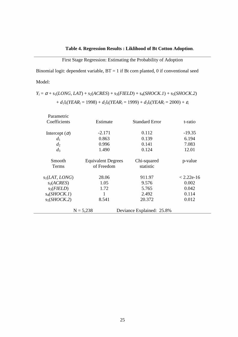
Regression Analysis

To examine these hypotheses more deeply, we use a two-step empirical procedure.

In the first step, we predict the likelihood of adopting Bt varieties of corn and cotton seed

using location, past yield shocks, and other covariates. In the second step, we examine

how the likelihood of adoption and past yield shocks relate to farmers’ stated reasons for

not adopting. Specifically, the second step examines the likelihood farmers who did not

adopt Bt cotton chose one of the two non-production-related reasons for this decision,

either trade or environment concerns (alternatives (2) or (4), as described above).

For both steps, we use a non-parametric generalized additive model (GAM). A

GAM, an non-parametric adaptation of the generalized linear model, is a flexible model

that relates smooth functions of covariates to any random dependent variable belonging to

the exponential family of distribution. For our model, we use the binomial logit to relate

our covariates to the probability of Bt adoption. Specifically, for the first step we assume

the adoption decision on field i is tied to a latent variable Yi that scales the utility of

adopting Bt varieties relative to the utility of using non-Bt seed varieties.

12

(1) Yi = α + s1(LONG, LAT) + s2(ACRES) + s3(FIELD) + s4(SHOCK.1) + s5(SHOCK.2) +

d1Ii (YEARi = 1999) + d2Ii(YEARi = 2000) + d3Ii (YEARi = 2001) + εi ,

Where LONG and LAT are the longitude and latitude of the field location, ACRES is the

farm-wide total number of acres planted to corn, FIELD is the number of acres in the field

sampled, SHOCK.1 and SHOCK.2 are the county yield shocks from the previous two

years, Ii(YEAR = X) is an indicator variable for the year the field was sampled (equal to 1

if the year is X and zero otherize), d1, d2, and d3 are fixed, unknown parameters, s1(),s2(),

and s3(), are smooth non-parametric functions, and εi an error that encapsulates unobserved

factors influencing adoption.

We use LAT, LONG, FIELD, ACRES, and YEAR as our primary covariates

because previous research suggests that these are variables are among the strongest

predictors of adoption (USDA-ERS). For most of our observations, we do not have

information on operator or other farm characteristics that are often included in adoption

equations. Rather than restrict our sample to the single year for these data are available,

we elected to include all observations from four years and use fewer explanatory variables.

We made this choice for several reasons. First, in previous studies farm-operator

characteristics, though statistically significant in some circumstances, were weak

predictors of adoption. Second, the spatial variables should pick up many unobservable

variables. Third, and most importantly, with only a single year of data the yield shocks

may be confounded by the spatial surface or other factors that vary spatially, so it was

important to use several years of adoption data. Fourth, because the weather-induced yield

13

shocks vary widely and unpredictably from year-to-year, they should be uncorrelated with

any factors excluded from our model, so their omission should not bias our regression.

For the second step, we consider farmers not adopting Bt corn in 2001 and examine

their rationale for not doing so. For this second step, we only examine corn farmers in

2001 because this is the only instance a question was asked regarding the reasoning non-

adoptors. We assume a farmer’s non-production-related rationale for not adopting Bt corn

(reason (2) or (4), as cited above) is tied to a latent variable Zi, where

(2) Zi = β + f1(LONG, LAT) + f2(ACRES) + f3(FIELD) + f1(Prob [Yi > 0]) +

f2(SHOCK.2) + f3(SHOCK.2* Prob [Yi > 0]) + ηi ,

the variables LONG, LAT, ACRES, FIELD, and Yi are defined as described above,

SHOCK.2 is the county-wide yield shock from two years prior (1999), and ηi is the error

that encapsulates unobserved factors. We assume both Yi and Zi have a logistic distribution

such that

Prob [Yi > 0] = exp(Yi) / (1 + exp(Yi))

and

Prob [Zi > 0] = exp(Zi) / (1 + exp(Zi)).

The smooth terms in this two-step model are estimated using penalized regression

splines with smoothing parameters selected by an unbiased risk estimator (UBRE). For a

general overview of these methods, see Wood (2001) and Wood and Augustin (2002). To

estimate the model we used a regression package “mgcv,” written by Wood, for the

14

statistical software R. This statistical software and package are available for free (see

http://www.r-project.org/).

Summaries of estimates of equation (1) for corn and cotton are reported in tables 3

and 4, respectively; a summary of estimates for equation (2) for corn is reported in table 5

(no data is available to estimate equation 2 for cotton). The summary tables report

estimates and standard errors of the fixed coefficients, equivalent degrees of freedom, and

overall statistical significance of the smooth terms, and the percent deviance explained, a

measure of overall fit akin to the R2 measure in continuous-response models.

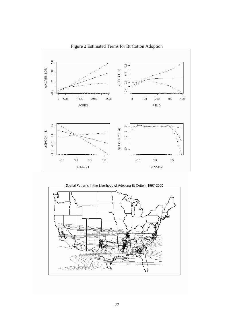
In figures 1, 2, and 3 we present plots of the estimated smooth functions together

with standard error bands (plus and minus two standard errors at each point). These plots

illustrate the marginal effects of the covariates. The hash lines on the bottom of each plot

show where the data lie. The vertical axis on these plots is the latent variable (Y in figure 1

and Z in figure 2), holding all other covariates at their population medians.

The two-dimensional spatial terms are plotted below the one-dimensional terms

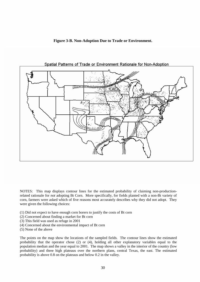
using contour maps that overlay maps of the United States. For these plots, the predicted

latent variables have been transformed into the predicted probability. For example, Figure

3-B displays contour lines for the estimated probability of claiming non-production-related

rationale for not adopting Bt Corn (either alternative (2) or (4), as described above). The

points on the map show the locations of the sampled fields. The contour lines show the

estimated probability that the operator chose (2) or (4), holding all other explanatory

variables equal to the population median and the year equal to 2001. The map shows a

valley in the interior of the country (low probability) and three high plateaus over the

northern plans, central Texas, the east. The estimated probability is above 0.8 on the

15

plateaus and below 0.2 in the valley. Note that this map holds all other explanatory

variables constant.

The earlier statistical tests show a correlation between negative yield shocks and

the citing of environmental or marketing concerns. By itself, this provides some evidence

of cognitive dissonance among the farmers that decided not to use Bt corn. After having

decided to not adopt, possibly due to a bad previous experience, these farmers may have

inflated their concerns about EU’s trade ban or environmental concerns to justify their

decisions ex-post. The statistics fail, however, to take account of other factors that may

cause these beliefs. For example, it may be that these beliefs are a result of the way media

portrayed these possibilities in the particular areas where bad yield shocks had occurred. In

fact the regression raises some doubt about whether this is the case. Here using a spatial

map as a control for previous disposition is a problem because this map may completely

represent local yield shocks from a single year (in this case 1999). Hence, there may be a

problem with multicolinearity. In fact, the regression reported in table 5 shows the yield

shocks to be insignificant, but positively related to citing non-production related reasons

for not using Bt corn. While this result does not rule out the existence of cognitive

dissonance, it provides little support for the hypothesis. More powerful tests would be

possible if more years of data regarding farmers’ reasons for non-adoption were available.

With more years of data, there would be less multicolinearity between the shocks and

location.

The map in figure 3-B raises other questions as to correlation with weather. Here

there appears to be a big split between central corn growing states (such as Iowa and

Illinois) where production problems were cited as the primary reason not to use Bt, and

more urban states (Ohio, Pennsylvania, North Carolina) where environmental and trade

16

restrictions were the primary concern. In fact, this map appears to display the exact inverse

of the map in Figure 2, which displays the marginal effect of location on the probability of

adoption. In other words, farmers were much more likely to react to problems with the

environment or trade if they are located in an area where there is a low concentration of

production. If farm operators were more prone to believe in trade problem or

environmental problems in areas that happened to have negative supply shocks in 1999,

our results may have been caused by spurious correlation.

More detail can be obtained by examining the longer series of adoption decisions

among cotton and corn farmers as related to previous weather shocks. By using the entire

panel of data from the first stage, we can more fully take advantage of the spatial map as a

control and compare to idiosyncratic yield shocks. The results for cotton are stark. In table

4 we see that after controlling for spatial effects, yield shocks from two years previous has

a significant effect on adoption decisions, while previous years yield has only a marginal

effect. Moreover, the graph in figure 2 suggests that this is a negative relationship. Thus, a

farmer, after experiencing a bad year, is more likely to adopt Bt cotton in the next year

cotton is planted on the field. This provides some evidence to counter the rational model of

adoption for several reasons. First, it appears the idiosyncratic yield shock has somehow

provided new information to the farmer, when yields are the result of a nearly stable

distribution (our shocks display no autocorrelation). In this case, the farmer may display

representativeness bias, placing too much weight on new observations, and underweighting

previous experience. This is consistent with the notion that Bt seeds are viewed as

insurance, as this behavior has been repeatedly observed in insurance markets.

Secondly, since these yield shocks are not autocorrelated, and primarily related to

weather, it is puzzling that farmers would react by adopting Bt. This suggests that farmers

17

suppose that they can change their fortunes by altering production decisions that are

unrelated to their poor performance. It would be difficult to reconcile this behavior with a

sound understanding of the mechanisms that affect the performance of Bt cotton. These

biases are confirmed in our examination of mono-croppers.

In examining the results for Bt corn, we find some evidence of the

representativeness effect, although table 3 shows that effect of yield hsocks it is not

significant. Though we cannot rule out the same effect, it is interesting that the effect is not

as strong with the larger sample corn provides. While cotton is grown in a few, widely

dispersed areas, it is spatially concentrated where it is grown. Corn, on the other hand is

grown throughout the US, by a much larger number of farmers. This is perhaps evidence of

the more effective information distribution mechanism for corn farmers. It may be that

irrational effects are the result of confusion and misinformation arising more often for

more localized or specialized crops. Even without significant effects for corn, these results

paint a consistent story that some portion of adoption is based on trying to overcome

uncontrollable and chance events.

Conclusion

Adoption of new innovations occurs almost exclusively in the absence of complete

information regarding costs and benefits. Perhaps this environment of confusion and

contradictions provides a perfect environment for subjective, and less than rational,

reasoning. Although our results provide some evidence of representativeness and the

illusion of control, we find weak evidence of cognitive dissonance among those

considering the use of Bt crops.

The evidence of representativeness and control biases is somewhat stronger in the

case of US cotton than corn. This may be a result of better extension and education efforts

18

regarding the use of Bt corn. Corn is a major crop grown on nearly all farm land in a large

number of contiguous states. Alternatively, cotton production is concentrated in a few

widely dispersed areas. One possibility is that strong behavioral effects are most likely to

be found among more isolated producers, where superior information may not travel as

fast, or be as widely published. Further research to document the contribution of heuristics

and behavioral effects to the diffusion of new technologies may lead to greater insight into

ways to help farmers correct these biases. Improved understanding of these effects can

help eliminate informational deficiencies and aid rational adoption decisions. Only with an

understanding of the heuristics and biases involved in changing production technologies

can we hope to overcome ungrounded perceptions about new technologies.

19

References

Alexander, C., J. Fernandez-Cornejo, and R. Goodhue. “Iowa Producers’ Adoption of Bio-

engineered Varieties.” Journal of Agricultural and Resource Economics 28(3): 580-

595.

Camerer, Colin. (1995). “Individual Decision Making.” in John H. Kagel and Alvin E.

Roth (eds.) The Handbook of Experimental Economics. Princeton, NJ: Princeton

University Press, 1995.

Feder, G. R.E. Just and D. Zilberman “Adoption of Agricultural Innovations in Developing

Countries: A Survey.” Economic Development and Cultural Change 34 (1985): 255 –

298.

Fernandez-Cornejo, J. and W. McBride. “Adoption of Bioengineered Crops.” USDA, ERS,

Agricultural Economic Report No. 810, 2002.

Festinger, L. A Theory of Cognitive Dissonance, Evanston, Ill.: Row Peterson, 1957.

Gilovich, T., R. Vallone, and A. Tversky "The hot hand in basketball: On the

misperception of random sequences," Cognitive Psychology, 17 (1985): 295-314.

Glauber, J W., and K J. Collins. “Risk Management and the Role of the Federal

Government,” in R. Just and R. Pope, eds., A Comprehensive Assessment of the Role of

Risk in U.S. Agriculture, Boston: Kluwer Academic Publishers, 2002, pp. 469-488.

Grether, D.M. “Bayes Rule as a Descriptive Model: The Representativeness Heuristic.”

Quarterly Journal of Economic 95(1980): 537 – 557.

Henslin, J. M. “Craps and magic.” American Journal of Sociology, 73 (1967):, 316-330.

20

Hogg, R.V. and A.T. Craig, Introduction to Mathematical Statistics 5th ed. Englewood

Cliffs, NJ: Prentice Hall, 1995

Hurvich, C. M., and Simonoff, J. S. (1998), "Smoothing Parameter Selection in

Nonparametric Regression Using an Improved Akaike Information Criterion" Journal

of the Royal Statistical Society B, 60, 271 -293.

Kahneman, D. and A. Tversky. “On the Psychology of Prediction.” Psychological Review

80 (1973): 237 – 251.

Langer, E. “The Illusion of Control.” In Kahneman, D., P. Slovic and A. Tversky (eds.),

Judgment under Uncertainty: Heuristics and Biases. New York: Cambridge University

Press, 1982, pp. 231 – 238.

Lybbert, T. C. B. Barrett, J. G. McPeak and W. K. Luseno, “Bayesian Herders: Optimistic

Updating of Rainfall Beliefs in Response to External Forecasts.” Department of

Applied Economics and Management, Cornell University, Working Paper, 2004.

Rogers, E. Diffusion of Innovations. Iowa Stat Agricultural Experiment Station Report no.

18. Ames: Iowa State University, 1957.

Roberts, M.J. and N. Key “Does Liquidity Matter to Agricultural Production? How

Transitory Yield Shocks Influence Subsequent Plantings.” In Just. R. E. and R.D.

Poper (eds.) A Comprehensive Analysis of the Role of Risk in US Agriculture. New

York: Kluwer Academic Press, 2002, pp.

SAS Manual LOESS

Schultz, T.W. “The Value of the Ability to Deal with Disequilibrium.” Journal of

Economic Literature 13 (1975): 827 – 46.

Stoppard, T. Rosencrantz and Guildenstern are Dead, New York: Grove Press, 1991.

21

Tversky, A. and D. Khaneman, "Belief in the law of small numbers," Psychological

Bulletin, 76 (1971): 105 – 110.

USDA, “Adoption of Genetically Engineered Crops in the U.S.” ERS website:

http://ers.usda.gov/Data/BiotechCrops/ , November 12, 2003.

Wason, P.C., “Reasoning About a Rule.” Quaterly Journal of Experimental Psychology.

20 (1968): 273 – 281.

Wood (2001) mgcv:GAMs and Generalized Ridge Regression for R. R News 1(2):20-25.

Wood and Augustin (2002) GAMs with integrated model selection using penalized

regression splines and applications to environmental modelling. Ecological Modelling

157:157-177

22

Table 1. Number in Sample Using Bt and Non-Bt Seed by Yield Shock Quartile

Yield Shock Quartile

First Quartile Second Quartile Third Quartile Fourth Quartile

Corn

Bt 255 538 444 489

Non-Bt 1726 2611 2074 2123

Cotton

Bt 359 359 527 503

Non-Bt 1145 722 802 1144

Source: Authors’ calculations based on data from USDA Production Practices surveys

(1997-2000 for cotton and 1998-2001 for corn).

23

Table 2. Reasons for Nonadoption (Crop Rotation)

Two Years Previous Yields

Reason Cited First

Quartile

Second Quartile Third Quartile Fourth Quartile

(1) Borers 216 221 224 204

(2) Market 46 74 65 38

(3) Refuge 8 7 11 13

(4) Environment 28 11 19 18

(5) Other 270 251 245 295

Farmers were asked which of five reasons most accurately describes why they did not adopt. They were given the following choices: (1) Did not expect to have enough corn borers to justify the costs of Bt corn (2) Concerned about finding a market for Bt corn (3) This field was used as refuge in 2001 (4) Concerned about the environmental impact of Bt corn (5) None of the above

24

Table 3. Regression Results : Liklihood of Bt Corn Adoption.

First Stage Regression: Estimating the Probability of Adoption

Binomial logit: dependent variable, BT = 1 if Bt corn planted, 0 if conventional seed Model:

Yi = α + s1(LONG, LAT) + s2(ACRES) + s3(FIELD) + s4(SHOCK.1) + s5(SHOCK.2) +

d1Ii(YEARi = 1999) + d2Ii(YEARi = 2000) + d3Ii (YEARi = 2001) + εi

Parametric

Coefficients

Estimate

Standard Error

t-ratio

Intercept (α) -2.015 0.064 -31.25 d1 0.249 0.087 2.86 d2 0.048 0.086 0.55 d3 0.334 0.081 4.14

Smooth Terms

Equivalent Degrees of Freedom

Chi-squared statistic

p-value

s1(LAT, LONG) 26.7 491.6 < 2.22e-16

s2(ACRES) 6.97 62.36 3.84e-11 s3(FIELD) 2.80 20.932 7.16e-05

s4(SHOCK.1) 2.1 1.4273 0.51356 s5(SHOCK.2) 1.313 0.95263 0.42979

N = 10,121 Deviance Explained: 10.6%

25

Table 4. Regression Results : Liklihood of Bt Cotton Adoption.

First Stage Regression: Estimating the Probability of Adoption

Binomial logit: dependent variable, BT = 1 if Bt corn planted, 0 if conventional seed Model: Yi = α + s1(LONG, LAT) + s2(ACRES) + s3(FIELD) + s4(SHOCK.1) + s5(SHOCK.2)

+ d1Ii(YEARi = 1998) + d2Ii(YEARi = 1999) + d3Ii(YEARi = 2000) + εi

Parametric

Coefficients

Estimate

Standard Error

t-ratio

Intercept (α) -2.171 0.112 -19.35 d1 0.863 0.139 6.194 d2 0.996 0.141 7.083 d3 1.490 0.124 12.01

Smooth Terms

Equivalent Degrees of Freedom

Chi-squared statistic

p-value

s1(LAT, LONG) 28.06 911.97 < 2.22e-16

s2(ACRES) 1.05 9.576 0.002 s3(FIELD) 1.72 5.765 0.042

s4(SHOCK.1) 1 2.492 0.114 s5(SHOCK.2) 8.541 20.372 0.012

N = 5,238 Deviance Explained: 25.8%

26

Figure 1 Estimated Terms for Bt Corn Adoption

Note: Red contour lines display estimated probability of adoption (see results reported in table 3) holding continuous covariates besides location (latitude and longitude) equal to population median and the year equal to 2001.

27

Figure 2 Estimated Terms for Bt Cotton Adoption

28

Table 5. Regression Results: Liklihood of Non-Production Influences

Second Stage Regression: Estimating the Probability of Non-production-related reason for NOT adopting BT Corn

Binomial logit: dependent variable = 1 if (alternative 2 or 4), 0 otherwise

Model:

Zi = β + f1(LONG, LAT) + f2(ACRES) + f3(FIELD) + f4(Prob [Yi > 0]) +

f5(SHOCK) + f6(SHOCK* Prob [Yi > 0]) + εi ,

Parametric Coefficients

Estimate

Standard Error

t-ratio

Intercept (β) -5.335 0.38 -14.04

Smooth Terms Equivalent Degrees of Freedom

Chi-squared statistic

p-value

f1(LONG, LAT) 29 77.06 3.09e-06

f2(ACRES) 8.018 48.69 7.44e-08 f3(FIELD) 3.424 44.84 1.90e-09

f4(Prob [Yi > 0]) 8.541 62.04 3.34e-10 f5(SHOCK) 1 0.053 0.8177

f6(SHOCK* Prob [Yi > 0]) 1 0.034 0.8535

N = 2315 Deviance Explained: 29.5%

29

Figure 3-One-Dimensional Smooth Terms from Table 5

30

Figure 3-B. Non-Adoption Due to Trade or Environment.

NOTES: This map displays contour lines for the estimated probability of claiming non-production-related rationale for not adopting Bt Corn. More specifically, for fields planted with a non-Bt variety of corn, farmers were asked which of five reasons most accurately describes why they did not adopt. They were given the following choices: (1) Did not expect to have enough corn borers to justify the costs of Bt corn (2) Concerned about finding a market for Bt corn (3) This field was used as refuge in 2001 (4) Concerned about the environmental impact of Bt corn (5) None of the above The points on the map show the locations of the sampled fields. The contour lines show the estimated probability that the operator chose (2) or (4), holding all other explanatory variables equal to the population median and the year equal to 2001. The map shows a valley in the interior of the country (low probability) and three high plateaus over the northern plans, central Texas, the east. The estimated probability is above 0.8 on the plateaus and below 0.2 in the valley.