THE IMPACT OF 401(K) PARTICIPATION ON THE WEALTH

DISTRIBUTION: AN INSTRUMENTAL QUANTILE REGRESSION

ANALYSIS

VICTOR CHERNOZHUKOV AND CHRISTIAN HANSEN

Abstract. In this paper, we use the instrumental quantile regression approach developed

in Chernozhukov and Hansen (2001) to examine the effects of 401(k) plans on wealth

using data from the Survey of Income and Program Participation. Using 401(k) eligibility

as an instrument for 401(k) participation, we estimate the quantile treatment effects of

participation in a 401(k) plan on several measures of wealth. The results show the effects of

401(k) participation on net financial assets are positive and significant over the entire range

of the asset distribution, and that the increase in the low tail of the assets distribution

appears to translate completely into an increase in wealth. However, there is significant

evidence of substitution from other forms of wealth in the upper tail of the distribution.

JEL Classification: H31, C21, C31

We would like to thank Jim Poterba, Byron Lutz, David Lyle, Ivan Fernandez and Whitney Newey for

helpful comments and suggestions. We are also grateful for comments from two anonymous referees and the

co-editor which substantially improved the presentation and content of the paper. All remaining errors are

ours.

1

1. Introduction

In the early 1980s, the United States introduced several tax deferred savings options in an

effort to increase individual saving for retirement. The two options which have generated the

most interest are Individual Retirement Accounts (IRAs) and 401(k) plans. Tax deferred

IRAs and 401(k) plans are similar in that both allow the individual to deduct contributions

from taxable income and allow tax-free accrual of interest on assets held within the plan.

The key differences between the two savings options are that employers provide 401(k) plans,

and employers may also match a certain percentage of an employee’s contribution. Since

401(k) plans are provided by employers, only workers in firms offering plans are eligible for

participation, while participation in IRAs is open to everyone.1

While it is clear that 401(k) plans and, to a lesser extent, IRAs are widely used as

vehicles for retirement saving, their impact on assets is less clear. The key problem in de-

termining the effect of participation in IRA and 401(k) plans on accumulated assets is saver

heterogeneity coupled with non-random selection into participation states. In particular,

it is generally recognized that some people have a higher preference for saving than oth-

ers. Thus, it seems likely that those individuals with the highest unobserved preference for

saving would be most likely to choose to participate in tax-advantaged retirement savings

plans and would also have higher savings in other assets than individuals with lower unob-

served saving propensity. This implies that conventional estimates that do not account for

saver heterogeneity and selection of the participation state will be biased upward, tending

to overstate the actual savings effects of 401(k) and IRA participation.

This problem has long been recognized in the savings literature and has led to numerous

important studies which attempt to overcome this problem. In a series of articles, Poterba,

2

Venti, and Wise (1994, 1995, 1996) use comparisons between groups based on eligibility

for 401(k) participation. They argue that 401(k) eligibility can be taken as exogenous

given income. The argument is motivated by the fact that eligibility is determined by the

employer, and so may be taken as exogenous conditional on covariates. Poterba, Venti,

and Wise (1996) contains an overview of suggestive evidence based on pre-program savings

used to substantiate this claim and reports mean and median regression estimates of the

impact of 401(k) eligibility on household net financial assets. The results show that 401(k)

eligibility has significant and positive effects on net financial assets. Based on the assumed

exogeneity of 401(k) eligibility, they attribute this difference to the causal effect of 401(k)

eligibility on savings.2 Recent work by Benjamin (2003) examines the effects of eligibility

on savings using matching based on the propensity score and finds positive, although much

more modest, effects of 401(k) eligibility on assets.3

A similar approach, which we follow in this paper, is that of Abadie (2003). Abadie,

assuming that eligibility for a 401(k) is exogenous given income (and other covariates), uses

401(k) eligibility as an instrument for 401(k) participation in order to estimate the effect of

401(k) participation, not eligibility, on net financial assets. Abadie uses a novel semipara-

metric estimator which estimates the average effect for compliers.4 Since only individuals

eligible for a 401(k) can participate, the average effect for compliers also corresponds to

the average effect for the treated. Abadie’s results suggest that the average effect for the

treated of 401(k) participation is significant and positive.

One drawback of all of these studies is that they focus the analysis on measures of central

tendency: the mean or the median. While the mean and median impacts are interesting

and important measures in determining a program’s impact, they are not sufficient to

fully characterize the impact of the treatment except under very restrictive conditions. In

3

particular, they are uninformative about the impact of the treatment on other, perhaps more

interesting, points in the outcome distribution when the treatment effect is heterogeneous.

Understanding the distributional impact of 401(k) plans is especially interesting from a

policy perspective since policy makers may be particularly concerned about the impact of

401(k) plans on the lower part of the wealth distribution. In addition, knowledge of the

distributional impact of a program provides a clearer picture of what is driving the mean

results.

As with estimates of the mean effect, the analysis of the distributional effect is compli-

cated by the possibility that individuals choose whether or not to participate in a 401(k)

based on their unobserved preferences for saving. One estimator which would allow a more

full characterization of the effect of a heterogeneous treatment given treatment exogeneity is

the quantile regression estimator of Koenker and Bassett (1978). However, the self-selection

of the participation state makes the conventional quantile regression estimator inappropri-

ate.5

In this paper, we contribute to the extensive set of existing literature of the impact of

401(k) plans on wealth by analyzing the impact of 401(k) participation on the entire wealth

distribution. Using the reasoning of Poterba, Venti, and Wise (1994, 1995, 1996) and Abadie

(2003) outlined above, we use 401(k) eligibility as an instrument for 401(k) participation in

order to estimate the effect of participating in a 401(k) on various measures of wealth. To do

this, we employ a model and an estimator developed in Chernozhukov and Hansen (2001).

The model provides a set of assumptions under which the conditional quantiles of the out-

come distribution may be recovered from a set of statistical moment equations through

the use of instrumental variables. The estimator we use is computationally convenient for

linear quantile models and can be computed through a series of conventional linear quantile

4

regressions. Chernozhukov and Hansen (2001) demonstrate that the estimator is consistent

under endogeneity and treatment effect heterogeneity. Thus, this paper provides an im-

portant complement to the work discussed above which focuses on estimating the impact

of 401(k) plans on the center of the outcome distribution. Also, due to the binary nature

of both the participation decision and the eligibility instrument, the approach developed

by Abadie, Angrist, and Imbens (2002) to estimate quantile effects for binary treatments

under endogeneity also applies. We present estimates obtained through both procedures to

provide both a robustness check and a comparison of the two approaches. We find that the

results are very similar using either estimation procedure.

The instrumental quantile regression estimates indicate that there is considerable het-

erogeneity in the effect of 401(k) participation on net financial assets, with the treatment

effect increasing monotonically as one moves from the lower to the upper tail of the asset

distribution. The results are also uniformly positive and significant, suggesting that 401(k)

participation positively impacts net financial assets across the entire distribution. The effect

of participation on total wealth is positive and approximately constant for all quantiles. In

addition, it is of the same magnitude as the effect of participation on net financial assets

for low quantiles, but is substantially smaller than the effect of participation on the upper

quantiles of net financial assets. These results suggest that the increase in net financial

assets observed in the lower tail of the conditional assets distribution can be interpreted as

an increase in wealth, while the increase in the upper tail of the distribution is mitigated by

substitution with some other component of wealth. The effect of participation on net non-

401(k) financial assets is uniformly insignificant, which suggests there is little substitution

for 401(k) assets along this dimension of wealth.6

5

The remainder of the paper is organized as follows. Section 2 reviews the model of

quantile treatment effects of Chernozhukov and Hansen (2001) and demonstrates how an

empirical model for assets may be embedded in the model. In Section 3, the data used in

the empirical analysis are described. Section 4 presents the empirical results and compares

the results from the estimator of Chernozhukov and Hansen (2001) to those obtained with

the estimator of Abadie, Angrist, and Imbens (2002), and Section 5 concludes.

2. An Instrumental Variable Model for Quantile Treatment Effects

In the following, we briefly present the assumptions and main implications of the instru-

mental variables model of quantile treatment effects developed in Chernozhukov and Hansen

(2001). We then show how an empirical model of savings decisions may be embedded in

this framework. This discussion helps illustrate the interpretation of the estimates of the

model, especially the interpretation of the quantile index τ , and isolates the key identifying

assumptions.

2.1. Potential Outcomes and the QTE. The model is developed within the conventional

potential (latent) outcome framework. Potential real-valued outcomes are indexed against

treatment d and denoted Yd. For example, Yd is an individual’s outcome when D = d.

Treatments d take values in a subset D of Rl. The potential outcomes Yd are latent

because, given the selected treatment D, the observed outcome for each individual or state

of the world is Y ≡ YD. That is, only one component of potential outcomes vector Yd is

observed for each observational unit.6

While there are many features of the distributions of potential outcomes that may be

interesting, we focus on the quantiles of potential outcomes conditional on covariates X,7

QYd

(τ |x), τ ∈ (0, 1)

,

and the quantile treatment effects (QTE) that summarize the difference between the quan-

tiles under different treatments (e.g. Doksum (1974)):

QYd(τ |x) − QY

d′(τ |x) or, if defined,

∂

∂dQYd

(τ |x).

Quantile treatment effects represent a useful way of describing the effect of treatment d on

different points of the marginal distribution of potential outcomes.

Typically D is selected in relation to Yd inducing endogeneity, so that the conditional

quantile of Y given the selected treatment D = d, denoted QY (τ |d, x), is generally not equal

to the quantile of potential or latent outcome QYd(τ |x). This makes the conventional quan-

tile regression inappropriate for the estimation of QYd(τ |x). The model of Chernozhukov and

Hansen (2001), briefly presented below, states the conditions under which we can recover

the quantiles of latent outcomes through a set of conditional moment restrictions.

2.2. The Instrumental Quantile Treatment Model. We build the model from the

basic Skorohod representation of latent outcomes Yd, which yields for each d given X = x

Yd = q(d, x, Ud), where Udd∼ U(0, 1), (2.1)

and q(d, x, τ) = QYd(τ |x) is the conditional τ -quantile of latent outcome Yd.

8 This repre-

sentation is essential to the rest of the analysis.

The variable Ud is responsible for heterogeneity of outcomes for individuals with the

same observed characteristics x and treatment d. It also determines their relative ranking7

in terms of potential outcomes. Hence we will call Ud the rank variable, and may think

of it as representing some innate ability or level of preference. This allows interpretation

of the quantile treatment effect as the treatment effect for people with a given rank in the

distribution of Ud, making quantile analysis an interesting tool for describing and learning

the structure of heterogeneous treatment effects.

The model consists of five main conditions (some are representations) that hold jointly.

The IVQT Model: Given a common probability space (Ω, F, P ), for P -almost every value

of X,Z, where X represents covariates and Z represents excluded instruments, the following

conditions A1-A5 hold jointly:

A1 Potential Outcomes. Given X = x, for each d, for some Udd∼ U(0, 1),

Yd = q(d, x, Ud),

where q(d, x, τ) is strictly increasing and left-continuous in τ .

A2 Independence. Given X = x,Ud

is independent of Z.

A3 Selection. Given X = x,Z = z, for unknown function δ and random vector V ,

D ≡ δ(z, x, V ).

A4 Rank Similarity. For each d and d′, given (V,X,Z)

Ud is equal in distribution to Ud′ .

8

A5 Observed variables consist of (for UD ≡ ∑d∈D

I(D = d) · Ud)

Y ≡ q(D,X,UD),

D ≡ δ(Z,X, V ),

X, Z.

Chernozhukov and Hansen (2001) demonstrate that the following result is an implication

of the IVQT model.

Theorem 1 (Main Statistical Implication). Suppose conditions A1-A5 hold. Then, for

any τ ∈ (0, 1), a.s.

P [Y ≤ q(D,X, τ)|X,Z] = τ and P [Y < q(D,X, τ)|X,Z] = τ. (2.2)

This result provides an important link of the parameters of the IVQT model to a set

of conditional moment equations which are used in Chernozhukov and Hansen (2001) to

develop identification conditions for the IVQT model as well as for estimation and inference.

In addition, Chernozhukov and Hansen (2001) give an extensive discussion of the IVQT

model, its assumptions, and its identification. While this discussion will not be repeated

here, it is important to note that the assumptions of the IVQT model differ from those in

other models with endogeneity and heterogeneous treatment effects in two key respects.9

First, the IVQT model imposes a different set of independence conditions; in particular,

it does not require that the instruments, Z, are independent of the errors in the selection

equation V . The independence of Z and V may be violated when Z is measured with error

or related to V in other ways. Second, the IVQT model imposes rank similarity, Assumption

A4, which will be discussed in the context of saving decisions below.9

2.3. The Instrumental Quantile Regression Model and Saving Decisions. As-

sumptions A1-A5 represent a plausible framework within which to analyze the effects of

participating in a 401(k) plan on an individuals accumulated wealth. First, wealth, Yd, in

the participation state d ∈ 0, 1 can be represented as

Yd = q(d,X,Ud), Ud ∼ U(0, 1)

by the Skorohod representation of random variables, where τ 7→ q(d,X, τ) is the conditional

quantile function of Yd and Ud is an unobserved random variable. Following the discussion

in Section 2.2, we will refer to Ud as the preference for saving and thus interpret the quantile

index τ as indexing rank in the preference for saving distribution.10 The individual selects

the 401(k) participation state to maximize expected utility:

D = arg maxd∈D

E[

WYd, d∣∣∣X,Z, V

]= arg max

d∈D

E[

Wq(d, x, Ud), d∣∣∣X,Z, V

], (2.3)

where Wy, d is the unobserved Bernoulli utility function. As a result, the participation

decision is represented by

D = δ(Z,X, V )

where Z and X are observed, V is an unobserved information component that depends on

rank Ud, and includes other unobserved variables that affect the participation state, and

function δ is unknown. Thus this model is a special case of the IVQT model. In this model,

the independence condition A2 only requires that Ud is independent of Z, conditional on

X.

The simplest form of rank similarity is rank invariance, under which the preference for

saving vector Ud may be collapsed to a single random variable:

U = U0 = U1.10

In this case, a single preference for saving is responsible for an individual’s ranking across

all treatment states. It is important to note that U is defined relative to observationally

identical people (individuals with the same X and Z). Rank invariance has been used

in many interesting models without endogeneity,11 and traditional simultaneous equations

models are built assuming rank invariance. However, as noted in Heckman and Smith

(1997), rank invariance may be implausible on logical grounds since it implies that the

potential outcomes Yd are not truly multivariate, but have a jointly degenerate distribution.

The similarity condition A4 is a more general form of rank invariance – it relaxes the

exact invariance of ranks Ud across d by allowing noisy, unsystematic variations of Ud across

d, conditional on (V,X,Z). This relaxation allows for variation in the ranks across the

treatment states, requiring only a “rank invariance in expectation”. Therefore, similarity

accommodates general multivariate models of outcomes. It states that given the information

in (V,X,Z) employed to make the selection of treatment D, the expectations of any function

of rank Ud does not vary across the treatment states. That is, ex-ante, conditional on

(V,X,Z), the ranks may be considered to be the same across potential treatments, but the

realized, ex-post, rank may be different across treatment states.

From an econometric perspective, the similarity assumption is nothing but a restriction

on the evolution on the unobserved heterogeneity component which precludes systematic

variation of Ud across the treatment states. Similarity allows interpretation of the quan-

tile treatment effect as the treatment effect holding the level of unobserved heterogeneity

constant across the treatment states:

q(d, x, τ) − q(d′, x, τ) = q(d, x, Ud) − q(d′, x, Ud′)∣∣∣Ud=Ud′=τ

.

11

Since changes in Ud across d are assumed to be asystematic, the quantile treatment effect

not only summarizes the distributional impact but also the actual likely treatment effect.

To be more concrete, consider the following simple example where

Ud = FV +ηd(V + ηd),

where FV +ηd(·) is the distribution function of V + ηd and ηd are mutually iid conditional

on V , X, and Z. The variable V represents an individual’s “mean” saving preference, while

ηd is a noisy adjustment.12 This more general assumption leaves the individual optimization

problem (2.3) unaffected, while allowing variation in an individual’s rank across different

potential outcomes.

While we feel that similarity may be a reasonable assumption in many contexts, imposing

similarity is not innocuous. In the context of 401(k) participation, matching practices

of employers could jeopardize the validity of the similarity assumption. This is because

individuals in firms with high match rates may be expected to have a higher rank in the

asset distribution than workers in firms with less generous match rates. This suggests that

the distribution of Ud may be different across the treatment states.

Similarity may still hold in the presence of the employer match if the rank, Ud, in the

asset distribution is insensitive to the match rate. The rank may be insensitive if, for ex-

ample, individuals follow simple rules of thumb such as target saving when they make their

savings decisions. Also, if the variation of match rates is small relative to the variation of

individual heterogeneity or if the covariates capture most of the variation in match rates,

then similarity will be satisfied approximately. Since the model is just-identified in our data,

specification tests based on the implications of Theorem 1 may not be used to perform overi-

dentifying tests. However, the quantile treatment effects model and estimator of Abadie,12

Angrist, and Imbens (2002), which apply only to binary treatment variables, provide a use-

ful robustness check. While the approach of Abadie, Angrist, and Imbens (2002) and the

approach presented in this paper generally identify and estimate different quantities, they

will estimate the same thing when the assumptions of both models, including similarity, are

satisfied and the set of compliers is representative of the population. If these conditions are

not met, then the two estimators will in general have different probability limits, suggesting

that a comparison of results based on the two models will provide evidence on the plausi-

bility of these assumptions. Comparisons between the two estimators are presented with

the empirical results in Section 4. The results from the two estimators are very similar,

suggesting that employer matching does not result in a serious violation of rank similarity.

3. The Data

To estimate the QTE, we use data on a sample of households from Wave 4 of the 1990

Survey of Income and Program Participation (SIPP).13 The sample is limited to households

in which the reference person is 25-64 years old, in which at least one person is employed,

and in which no one is self-employed.14 The sample consists of 9,915 households and all

dollar amounts are in 1991 dollars.

The 1991 SIPP reports household financial data across a range of asset categories. These

data include a variable for whether a person works for a firm that offers a 401(k) plan.

Households in which a member works for such a firm are classified as eligible for a 401(k).

In addition, the survey also records the amount of 401(k) assets. Households with a positive

401(k) balance are classified as participants, while eligible households with a zero balance

are considered non-participants.13

While there are several potential measures of wealth in the 1991 SIPP, we choose to focus

our analysis on total wealth, net financial assets, and net non-401(k) financial assets. Net

non-401(k) assets are defined as the sum of checking accounts, U.S. saving bonds, other

interest-earning accounts in banks and other financial institutions, other interest-earning

assets (such as bonds held personally), stocks and mutual funds less nonmortgage debt,

and IRA balances. Net financial assets are net non-401(k) financial assets plus 401(k)

balances, and total wealth is net financial assets plus housing equity and the value of

business, property, and motor vehicles.15

We use the same set of covariates as Benjamin (2003). Specifically, we use age, income,

family size, education, marital status, two-earner status, defined benefit (DB) pension sta-

tus, IRA participation status, and home ownership status. Marital status, two-earner sta-

tus, DB pension status, IRA participation status, and home ownership status are binary

variables, where two-earner status indicates whether both household heads, where present,

contribute to household income and DB pension status indicates whether the household’s

employer offers a DB pension plan. The education variable measures the number of years

of school completed by the household reference person, and for the analysis we have catego-

rized this variable into four groups: less than 12 years of education, 12 years of education,

13-15 years of education, and 16 or more years of education. Households are classified as

IRA participants if they have positive IRA asset balances, and households are classified

as home owners if the household has a positive home value. In addition, in the estimates

reported below, we control for age using categorical variables: less than 30 years old, 30-35

years old, 36-44 years old, 45-54 years old, and 55 years old or older. Following Poterba,

14

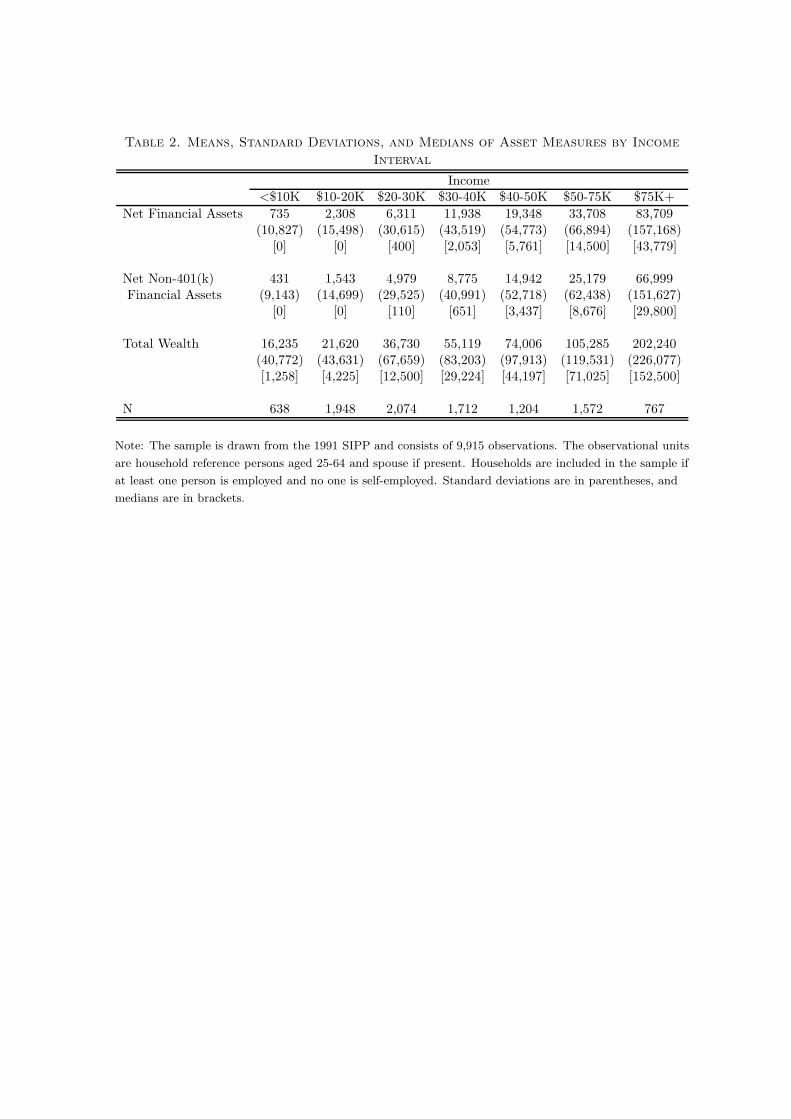
Venti, and Wise (1995), we control for income through the use of seven categorical vari-

ables. The income intervals are as follows: <$10K, $10-20K, $20-30K, $30-40K, $40-50K,

$50-75K, and $75K+.

[Insert Table 1 about here.]

[Insert Table 2 about here.]

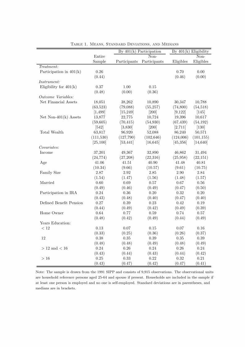
Table 1 contains descriptive statistics for the full sample as well as by eligibility and

participation status. 37% of the sample is eligible for a 401(k) plan while 26% choose to

participate. Among those eligible for a 401(k) account, the participation rate is 70%. The

descriptive statistics indicate that participants have larger holdings of all measures of wealth

that we consider. As expected, the means of all of the wealth variables are substantially

larger than their medians, indicating the high degree of skewness in wealth. The means also

show that 401(k) participants have more income, are more likely to be married, are more

likely to have IRAs and defined benefit pensions, are more likely to be home-owners, and

are more educated than non-participants. Average age and family size are similar between

the two groups. Descriptive statistics for the dependent variables by income category are

also provided in Table 2.

4. Empirical Results

4.1. Estimation and Inference Procedures. To capture the effects of 401(k) participa-

tion on net financial assets, we estimate linear quantile models of the form

QYd|X(τ) = dα(τ) + X ′β(τ)

where d indicates 401(k) participation status and is instrumented for by 401(k) eligibility,

following Abadie (2003) and Poterba, Venti, and Wise (1994, 1995, 1996).16 The outcomes Y15

are the three previously mentioned measures of wealth (total wealth, net financial assets, and

net non-401(k) financial assets), and X consists of dummies for income category, dummies

for age category, dummies for education category, a marital status indicator, family size,

two-earner status, DB pension status, IRA participation status, home ownership status,

and a constant.17 To more fully control for income, we also consider estimates obtained

within each income category. In these cases, the income category dummies are omitted and

a linear term in income is included to account for any remaining variation within income

category.

The main results reported below are for the standard quantile regression (QR) estimator

and the instrumental quantile regression (IQR) estimator of Chernozhukov and Hansen

(2001) which corrects for the endogeneity of 401(k) participation under the assumptions of

the model presented in Section 2 of this paper. The IQR estimator may be viewed as a

convenient method of approximately solving the sample analog of moment equations (2.2):18

1

n

n∑

i=1

(1(Yi ≤ D′iα + X ′

iβ) − τ)(X ′i , Z

′i)′ = op

(1√n

). (4.1)

When there is only one endogenous regressor and the model is just identified, the IQR

estimator for a given quantile may be computed as follows:

1. Run a series of standard quantile regressions of Y − Dαj on covariates X and

instrument Z where αj is a grid over α.

2. Take the αj that minimizes the absolute value of the coefficient on Z as the estimate

of α, α. Estimates of β, β, are then the corresponding coefficients on X.

In Chernozhukov and Hansen (2001), we show that, under regularity conditions and for

θ = [α, β′]′,

√n(θ − θ)

d→ N(0, J−1Ω(J−1)′),16

where, for Ψ = [Z,X ′]′ and ε = Y − Dα − X ′β,

Ω = τ(1 − τ)EΨΨ′ and J = E[fε(0|D,X,Z)Ψ[D,X ′]].

Chernozhukov and Hansen (2001) also provides further details covering estimation and

asymptotic theory in the general, potentially overidentified model.

Estimates of the QTE, α(τ), for many different points τ also provide an estimate of the

QTE process α(·) which treats α as a function of τ .19 Knowledge of the QTE process allows

formal testing of a number of interesting hypotheses. These include the constant effect

hypothesis (α(·) = α), of which the hypothesis of no effect (α(·) = 0) is a special case, and

the hypothesis of no endogeneity (α(·) = αQR(·) where αQR denotes the ordinary quantile

regression estimate). If the constant effect hypothesis is not rejected, the distributional

impact of the treatment may be captured by a single statistic, such as the mean or the

median treatment effect. Also, failure to reject the hypothesis of no endogeneity suggests

that the endogeneity bias is not statistically important and that standard QR estimates

may be used. Chernozhukov and Hansen (2002) provides asymptotic theory for the IQR

process and suggests a computationally attractive method for performing inference on the

IQR process.

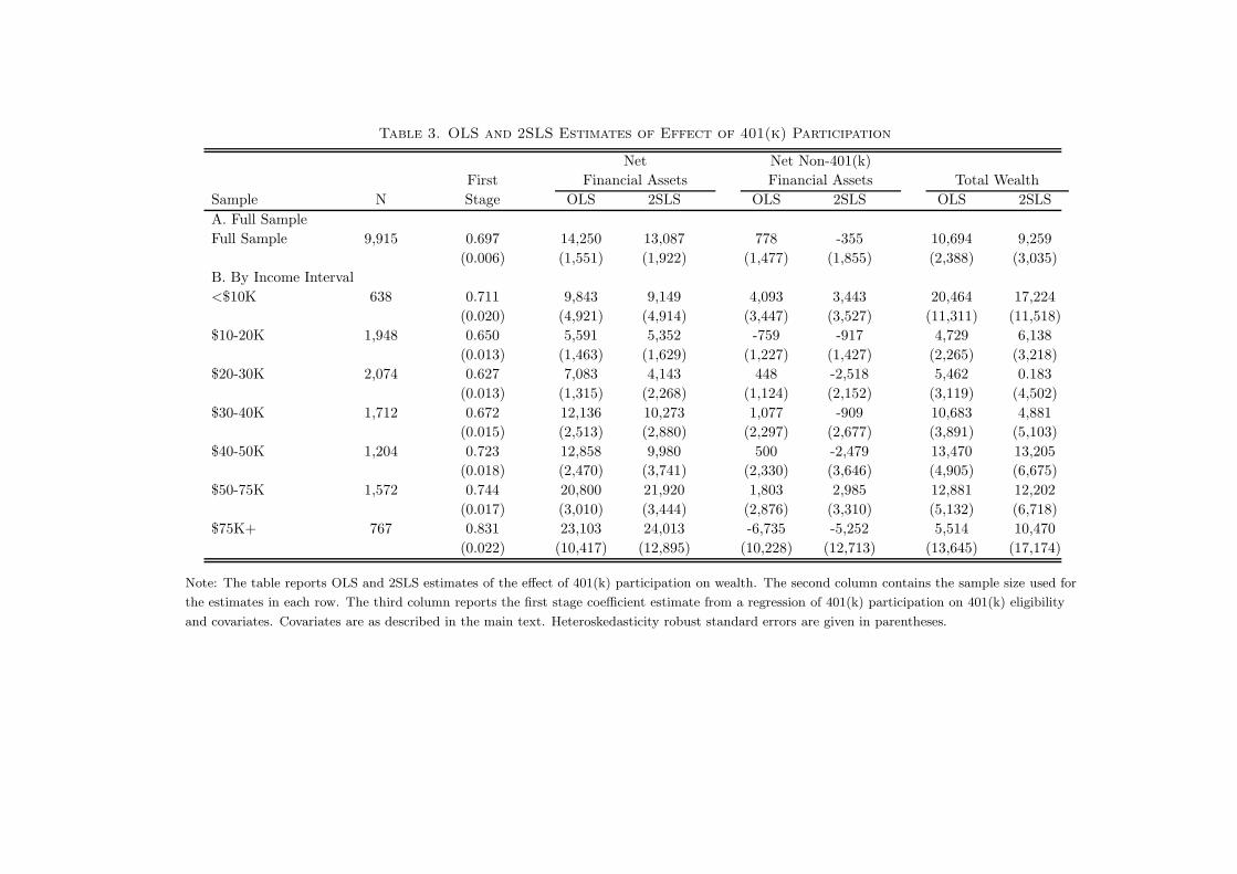
4.2. OLS and 2SLS Results. Table 3 provides OLS and 2SLS results of the participation

effect. These estimates serve as a benchmark for the quantile and instrumental quantile

regression estimates presented later. In addition, they are interesting in their own right.

Indeed, in the case of a constant treatment effect, these estimates would be sufficient to

fully characterize the distributional impact of the treatment.20

[Insert Table 3 about here.]17

The first stage estimates, reported in the third column of Table 3, confirm that eligi-

bility for a 401(k) is highly correlated with participation. In the full sample and within

each income category, the first stage estimate is large, positive, and highly significant. In-

deed, conditional on eligibility, the rest of the covariates have very small effects on 401(k)

participation.

In the full sample, the 2SLS estimates are uniformly smaller than the OLS estimates,

confirming the intuition that the OLS estimates should be upward biased. However, the

biases appear to be modest, especially when compared to the standard errors of the esti-

mates. After accounting for endogeneity, the impact of 401(k) participation on both total

wealth and net financial assets remains large and significant. Relative to the means, 401(k)

participation increases net financial assets by approximately 70% and total wealth by ap-

proximately 14%. The magnitude of both effects is also quite similar, though slightly larger

for net financial assets, suggesting little substitution between 401(k) assets and other forms

of wealth. On the other hand, 401(k) participation has relatively little impact on net non-

401(k) financial assets. Neither the OLS nor the 2SLS estimate of the effect of participation

on net non-401(k) financial assets is significantly different from zero, and both are quite

small in magnitude. Overall, these results suggest that the majority of the increase in net

financial assets may be attributed to new saving due to 401(k) plans and not to substitution

from other forms of wealth.

The results by income category provide additional evidence on substitution patterns. The

loss of precision resulting from estimating the treatment effect within income categories

makes drawing any firm conclusion difficult, but the patterns of the estimates are still quite

interesting.21 The impact of 401(k) participation on net financial assets is uniformly positive

and significant and tends to increase as one moves from lower to higher income categories.

18

This result appears to be consistent with the resource constraints of the different income

groups. The results for net non-401(k) financial assets are never significantly different from

zero. However, in all cases but one, the point estimate is negative and non-negligible, which

provides weak evidence that there is financial asset substitution that was obscured in the

results obtained in the full sample. While the results for total wealth show much less of a

pattern as one looks across income categories, it can be seen that in no case is the effect

significantly different from zero. The point estimates are uniformly positive and, in the

majority of cases, are reasonably large. This again provides weak evidence that 401(k)

participation increases total wealth by a modest amount, but that this increase is smaller

than the increase to net financial assets, indicating substitution between 401(k) and other

assets.

4.3. Quantile Regression and Instrumental Quantile Regression Results: Full

Sample. While the OLS and 2SLS results presented above provide a summary statistic

for the impact of the treatment, they fail to capture the distributional impact of 401(k)

participation on wealth. To further explore the effect of 401(k) participation on wealth,

we report results obtained from both standard quantile regression and the instrumental

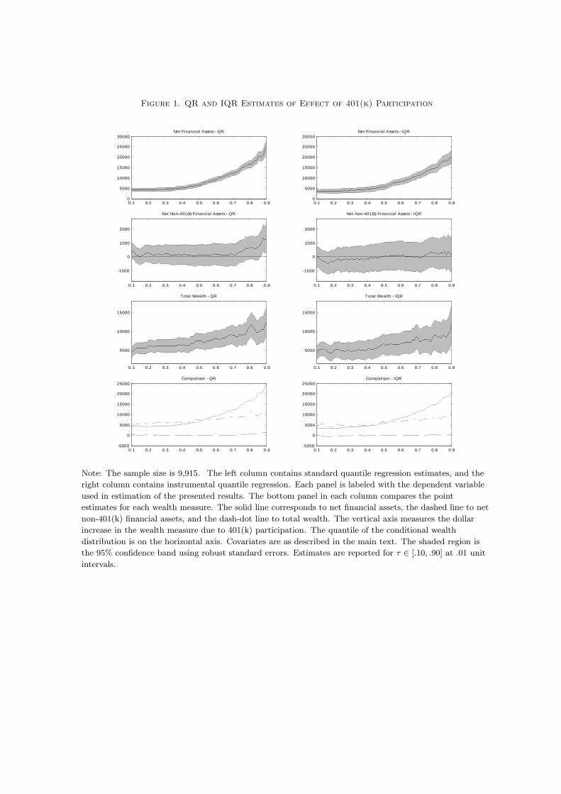
quantile regression of Chernozhukov and Hansen (2001) in Figure 1.

[Insert Figure 1 about here.]

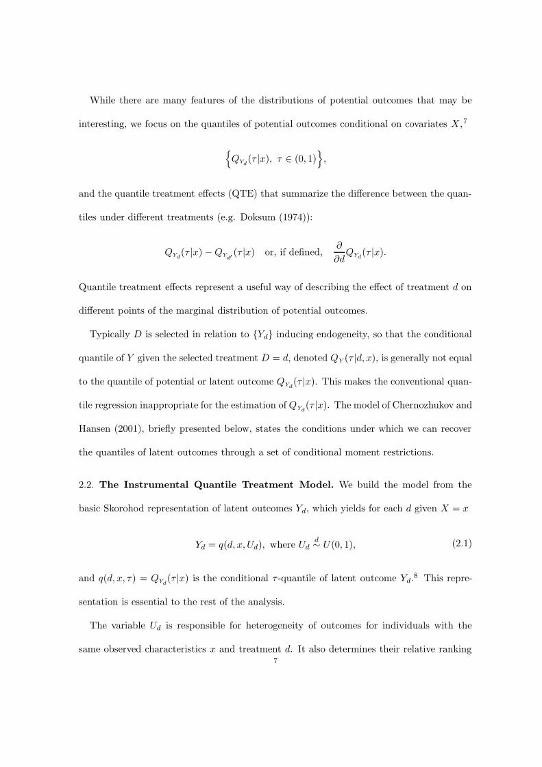
The left column of Figure 1 contains QR estimates of the effect of 401(k) participation

on the wealth measures, and the right column of Figure 1 presents the IQR estimates of

the QTE. The shaded region in the first six panels represents the 95% confidence interval.22

The last two panels plot the estimated effects for each of the dependent variables together19

to provide a comparison of the magnitudes and to facilitate the discussion of substitution

between the different wealth measures.

The results exhibit a number of striking features. First, the difference between the QR

and IQR estimators is not dramatic. Both exhibit the same pattern of results, though there

is some upward bias evident in the QR estimates. This bias is most evident in the estimates

for net financial assets and net non-401(k) financial assets, but is hardly noticeable in the

total wealth results.

Another interesting feature of the results is that the effect of participation on net financial

assets is highly non-constant, appearing to increase monotonically in the quantile index.

This result suggests that, conditional on income and other observables, people who rank

higher in the conditional wealth distribution are impacted far more than those ranking lower

in the conditional distribution. In addition, the effect is strongly positive across the entire

distribution. While these results correspond to our intuition, there is actually no other a

priori reason to believe that net financial assets must react in this way. In particular, if

people were simply substituting financial assets held in 401(k)s for other forms of financial

assets, the effect of 401(k) participation on net financial assets would be zero. These results

provide strong evidence against this hypothesis at all quantiles.

The impact of 401(k) participation on total wealth relative to its impact on net financial

assets also provides interesting insights. As with net non-401(k) financial assets, the effect

of participating in a 401(k) on total wealth is roughly constant, though in this case it is

uniformly positive. The most interesting feature of the effect on total wealth is that for

low quantiles it is of almost the same magnitude as the effect on net financial assets, while

it is substantially smaller than the effect on net financial assets in the upper tail of the

distribution. Taken together, these findings suggest that the increase in net financial assets

20

observed in the lower tail of the conditional assets distribution can be interpreted as an

increase in wealth, while the increase in the upper tail of the distribution is being mitigated

by substitution with some other (non-financial) component of wealth. However, even for

the highest quantiles, the substitution does not appear to be complete.

A final outstanding feature of the results is the indication that 2SLS estimates substan-

tially overstate the treatment effect across a large range of the net financial asset distribu-

tion. In fact, the 2SLS estimates of the treatment effect on net financial assets correspond

much more closely to the treatment effect at the 75th percentile of the distribution than to

that of the median.

[Insert Table 4 about here.]

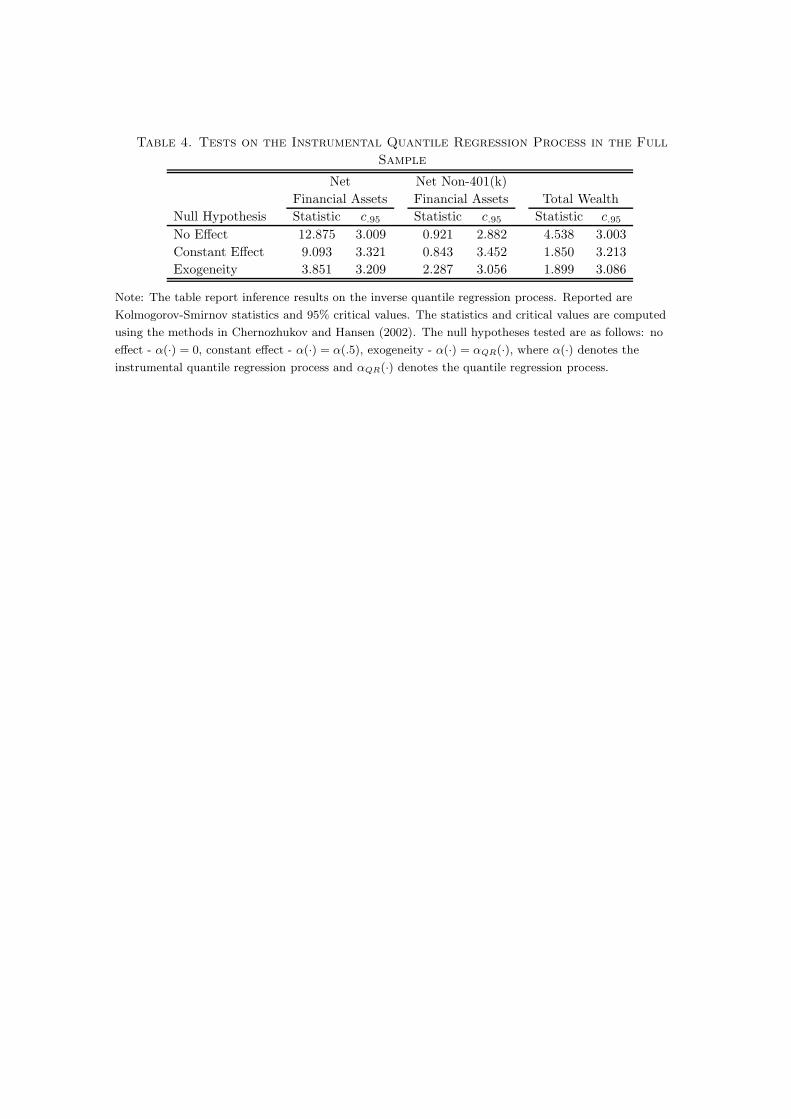
In order to strengthen and further develop our conclusions, we present test results based

on the empirical instrumental quantile regression process computed using the methods of

Chernozhukov and Hansen (2002). Kolmogorov-Smirnov (KS) test statistics and 95% crit-

ical values are given in Table 4. The test results lend further support to the conclusions

already drawn. The tests strongly reject the hypothesis that the impact of 401(k) par-

ticipation on net financial assets is constant and confirm that the impact is significantly

different from zero. In addition, we see that the hypothesis of exogeneity of treatment is

rejected for net financial assets. However, the tests fail to reject both the hypothesis of a

constant treatment effect (equal to the median effect) and the hypothesis of exogeneity for

total wealth and net non-401(k) financial assets. That the treatment effect for both total

wealth and net non-401(k) financial assets is statistically constant adds further credibility

to the conclusion that there is little substitution between 401(k) assets and other forms of

wealth in the low tail of the assets distribution but that there is substantial substitution in21

the upper tail. In addition, the results of the exogeneity tests provide some evidence that

there is endogeneity bias in the conventional QR estimates of the treatment effects.

4.4. Quantile Regression and Instrumental Quantile Regression Results: By In-

come Interval. As with analysis of the mean effect presented above, additional insights

about the QTE may be gained by examining the effect of 401(k) participation on our chosen

wealth measures within income interval. The independence assumption, A2, may also be

more plausible within income categories due to the finer conditioning on income, since the

arguments of Poterba, Venti, and Wise (1995) suggest that 401(k) eligibility is as good as

randomly assigned once income is conditioned upon. Of course, the estimates within in-

come category do suffer from a loss of precision relative to estimates obtained with a coarser

income control, which makes drawing firm inferences more difficult.

[Insert Figure 2 about here.]

[Insert Figure 3 about here.]

[Insert Figure 4 about here.]

[Insert Figure 5 about here.]

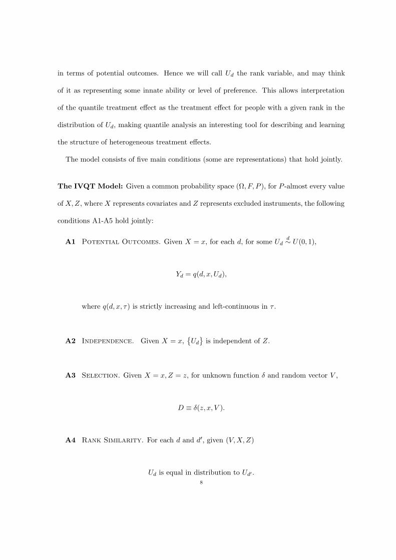
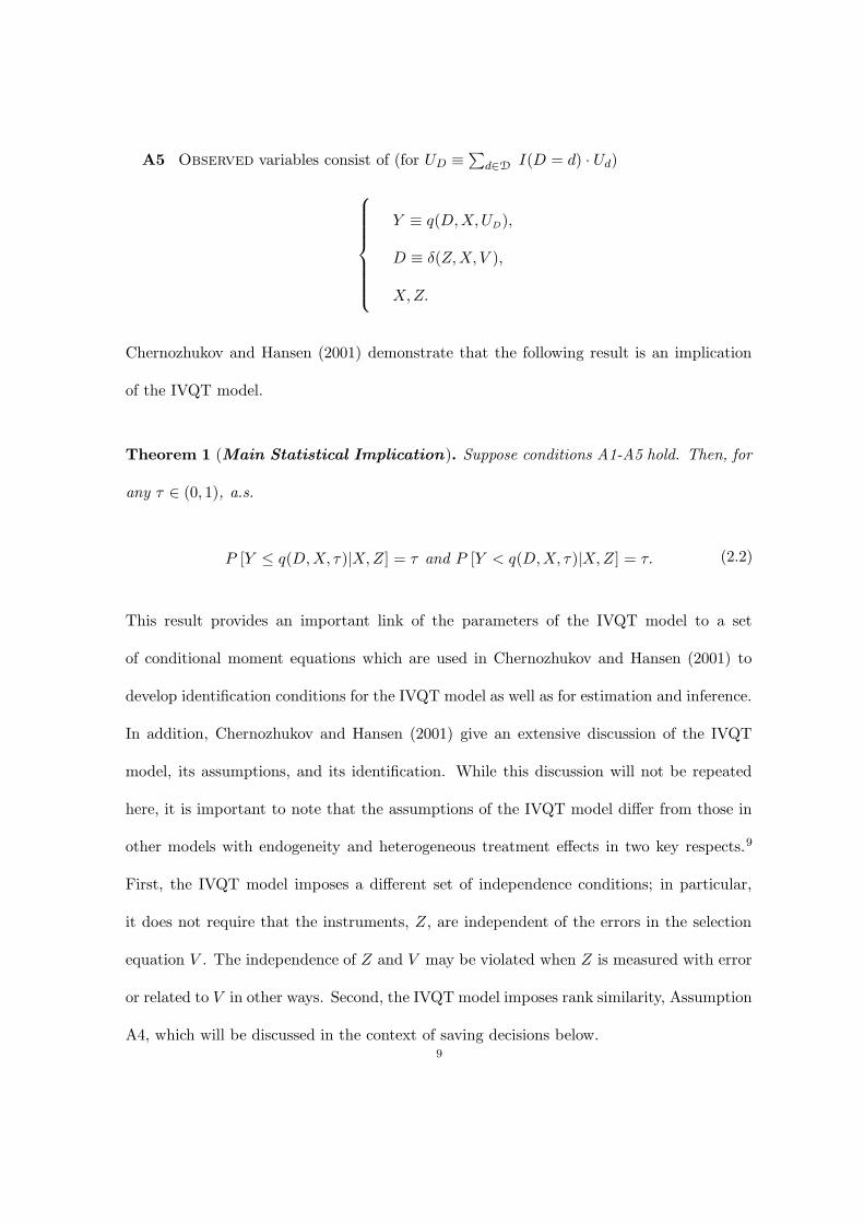
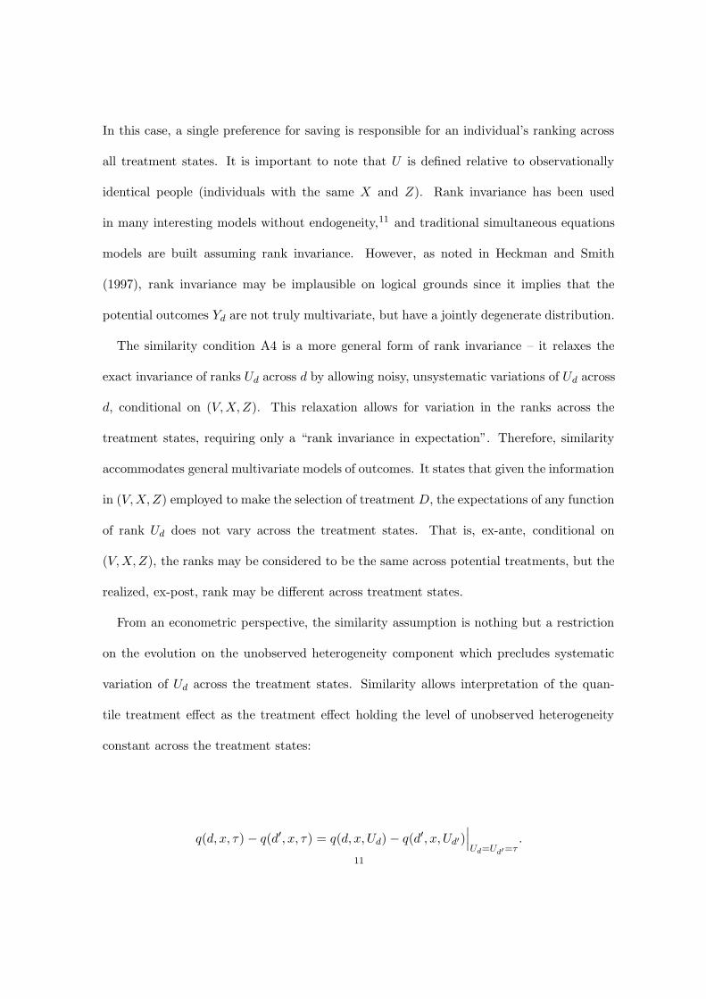
IQR estimation results by income category are reported in Figures 2-5.23 The figures

are arranged by dependent variable, with Figure 2 corresponding to net financial assets,

Figure 3 to net non-401(k) financial assets, and Figure 4 to total wealth. In all cases,

the shaded region represents the 95% confidence interval.24 Figure 5 contains plots of the

estimated effects for each of the dependent variables together to facilitate comparison of

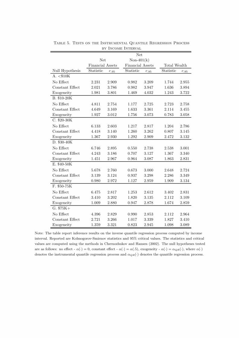
the magnitudes. Table 5 reports process test results.

[Insert Table 5 about here.]22

Within income categories, the results for net financial assets follow roughly the same

pattern as the results in the full sample. In all categories, the results are generally increasing

in the quantile index, and in all but the first income category, the process tests reveal that

the treatment effect is different from zero. In addition, the hypothesis of a constant effect is

rejected in all but the first and last income categories. As would be expected, the magnitudes

of the results increases as income increases. The point estimates in the first category are

close to zero across the majority of the quantiles, suggesting that participation in a 401(k)

has little effect on those with incomes of less than $10,000. Also, in each income interval,

the results are fairly constant and quite modest for quantiles below the median. Overall,

these results indicate that 401(k) participation increases accumulated net financial assets

in all, excepting possibly the first, income categories, but that these effects may be quite

modest through much of the distribution.

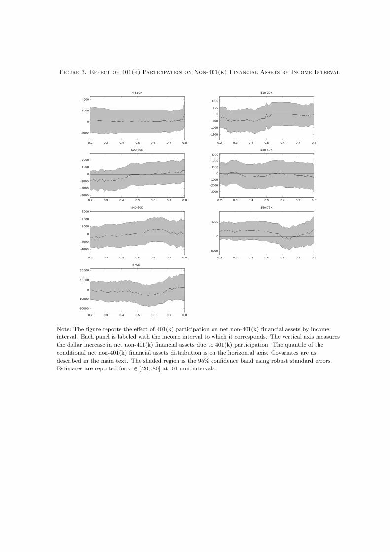
As with the results in the full sample, the estimated treatment effect of 401(k) partici-

pation on net non-401(k) financial assets is not significantly different from zero in any case.

The point estimates are also generally quite small, though they do exhibit some tendency

to be negative more often than positive. This negative tendency provides weak evidence

for some substitution between financial assets held in 401(k)s and other forms of financial

assets. That this negative tendency appears to be most pronounced for low quantiles also

suggests that those with low preferences for saving, who probably have relatively little in

the form of financial assets, are choosing to accumulate assets within 401(k)s instead of

elsewhere, whereas those with higher preferences for saving are saving in both locations.

The results for the effect of 401(k) participation on total wealth are the most varied across

income categories, though the lack of precision makes comparison difficult. One result which

is quite interesting is that, within the lowest income category, there appear to be extreme

23

outliers in the upper tail of the distribution. Examining the quantile results within the

first income category suggests there is little effect of 401(k) participation on wealth across

the majority of the wealth distribution. However, at approximately the 60th percentile, the

effects increase dramatically. These large effects in the upper tail also explain the anomalous

OLS and 2SLS results within the first income category illustrated in Table 2. The process

test of no effect does not reject within the first income category, which seems to be a plausible

conclusion given the small effect for most quantiles. It is also interesting that in the highest

income category the estimated participation effect on total wealth is close to zero in the

upper quantiles of the wealth distribution while the estimated effect on net financial assets

is quite large, suggesting a large amount of substitution in these quantiles. Overall, it is

difficult to draw any firm conclusions due to large estimated standard errors of the effects.

However, one robust finding seems to be that the estimated effect of participation on total

wealth and the estimated effect of participation on net financial assets are quite similar in

the lower tail of the wealth distribution, which suggests that participation in 401(k) plans

stimulates asset accumulation of those with low preferences for saving.

A final interesting note is that, within income categories, the hypothesis of the exogeneity

of 401(k) participation is never rejected. This could be because, conditional on income and

other covariates, 401(k) participation is as good as randomly assigned, or it could be driven

by small sample size and the lack of precision of the estimates. We choose to focus on the

IQR estimates because they are robust to endogeneity, but there is no statistical evidence

that endogeneity is present.

4.5. Comparison with Abadie, Angrist, and Imbens (2002). One key criticism of the

approach pursued thus far in this paper is that employer matching practices may invalidate24

the similarity assumption required in the model in Section 2. However, since both the

instrument and endogenous variable are binary, the model and approach of Abadie, Angrist,

and Imbens (2002) apply. A comparison between the results from the two approaches then

provides a specification check of the developed results.

The estimator of Abadie, Angrist, and Imbens (2002) is developed within the LATE

framework of Imbens and Angrist (1994). In particular, Abadie, Angrist, and Imbens

(2002) show that if

1. the instrument Z is independent of the outcome error, Ud in our notation, and the

error in the selection equation, V in our notation,

2. monotonicity, P (D1 ≥ D0|X) = 1 where D1 is the treatment state of an individual

when Z = 1 and D0 is defined similarly, holds,

3. and other standard conditions are met,

then the QTE for compliers, those individuals with D1 > D0, is identified and develop

an estimator for the QTE for compliers. Since only individuals eligible for a 401(k) can

participate, monotonicity holds trivially, and the QTE for compliers corresponds to the

QTE for the treated, which will correspond to the quantity identified by the IVQT model

of Section 2 if the treated are representative of the population and the assumptions of the

IVQT model are satisfied.

[Insert Figure 6 about here.]

Given that the two models are mutually compatible under the conditions outlined above

and the monotonicity assumption of Abadie, Angrist, and Imbens (2002) holds in the case

of 401(k) participation, a comparison of the previous results obtained via IQR and results25

obtained via the estimator of Abadie, Angrist, and Imbens (2002) provides a useful robust-

ness check of the previous results and the assumptions that underlie their interpretation.

Figure 6 reports results from the estimator of Abadie, Angrist, and Imbens (2002) in the

full sample and comparisons with corresponding IQR estimates.25 From this exercise, we

see that the pattern of results obtained from the two estimators are quite similar, with the

major differences being that the Abadie, Angrist, and Imbens (2002) estimates of the effects

of 401(k) participation on total wealth and on net non-401(k) financial assets appear to be

even more constant than those obtained through IQR.26

It appears that the difference in the estimates is small relative to sampling variation and

that one would not draw substantively different conclusions from either set of estimates.

The striking similarity between the estimates provides further support for the IQR results

discussed above and strongly suggests that employer matching of 401(k) contributions does

not result in failure of rank similarity.

4.6. Overall Conclusions and Cautions. Overall, the results indicate that 401(k) par-

ticipation has a positive impact on the accumulation of net financial assets. The results

suggest that the effect on net financial assets is increasing as one approaches the upper

tail of the net financial asset distribution. Estimates for the effect of 401(k) participation

on total wealth and net non-401(k) financial assets are approximately constant and indi-

cate that 401(k) participation generally increases total wealth but has little effect on net

non-401(k) financial assets. We interpret these results as indicating that participation in

401(k)s increases total wealth and that there is little substitution between financial assets in

401(k)s and other financial assets. In addition, the results suggest that there is substitution

between assets held in 401(k)s and other components of wealth in the upper tail of the26

wealth distribution, but that most financial assets held in 401(k)s in the lower tail of the

distribution represent new savings. This has important policy implications, as the people

in the low tail of the net financial asset distribution are also likely to be the people with

the lowest retirement savings.

The estimates also clearly indicate the inability of a single summary statistic, such as the

2SLS regression estimate of the treatment impact, to provide a clear picture of the impact of

a program on the distribution of the outcomes of interest. The 2SLS estimate for the effect

of 401(k) participation on net financial assets appears to overstate the actual treatment

across much of the distribution, corresponding most closely to the estimates for the upper

tail of the asset distribution. In addition, the single summary statistic provided by 2SLS

or OLS obscures the regions where divergences between the effect of 401(k) participation

on the different wealth measures occur and thus do not provide as full a description of the

program impact as the quantile-based methods.

While we feel that this paper provides insight into the effect of 401(k) participation on

wealth, it does suffer from limitations. First, all of the dependent variables used in this

analysis represent stocks of assets rather than the flow of savings. The accumulated level of

assets is interesting because it provides a summary of a person’s wealth and the resources

that are available to the individual. However, they are not sufficient to capture the effect

of the program on savings. In particular, given employer matching and the tax-advantaged

nature of 401(k) saving, it may be possible to have a large increase in accumulated assets

with little change in the individual’s flow of savings. Second, the data available in the

SIPP do not report all sources of pension wealth. In particular, the SIPP does not contain

information on assets held in DB plans or defined contribution plans other than IRAs and

401(k)s. The lack of these data could potentially bias the results upward if 401(k) assets

27

are substituting for these other forms of assets. While evidence from Poterba, Venti, and

Wise (2001) and Papke, Peterson, and Poterba (1996) is consistent with the view that

401(k)s rarely cause DB termination, it does not preclude substantial substitution between

the different forms of pensions.

5. Conclusion

In this paper, we apply the instrumental quantile regression model and estimators devel-

oped in Chernozhukov and Hansen (2001) and Chernozhukov and Hansen (2002) to data

from the SIPP, which has previously been used by Poterba, Venti, and Wise (1996), Abadie

(2003), Benjamin (2003), and Engen, Gale, and Scholz (1996), to examine the effects of

401(k) plans on savings. Following Poterba, Venti, and Wise (1996), Abadie (2003), and

Benjamin (2003), we use 401(k) eligibility as an instrument for 401(k) participation to es-

timate the QTE of participation in a 401(k) plan on various wealth measures. The QTE

provide a more full characterization of the effect of 401(k) participation on savings than

do conventional IV methods and supplement these methods by providing a more detailed

description of the distributional impact of 401(k) program participation.

The IQR estimates suggest that the effect of 401(k) participation on net financial assets is

quite heterogeneous, with the largest returns accruing to those who are in the upper tail of

the assets distribution. The results also indicate that the effect of 401(k) participation on

net financial assets is positive and significant over the entire range of the asset distribution

and that the effect is monotonically increasing in the quantile index. Effects on total wealth

and net non-401(k) financial assets, on the other hand, appear to be constant, and the effect

on net non-401(k) financial assets is not significantly different from zero while the effect on

total wealth is positive and significant. Overall, the results suggest that participation in28

401(k)s increases net financial assets across the asset distribution, but that this effect is

mitigated by substitution with other forms of wealth in the upper tail of the distribution.

They also demonstrate that estimates of treatment effects which focus on a single feature

of the outcome distribution may fail to capture the full impact of the treatment and that

examining additional features may enhance our understanding of the economic relationships

involved.

29

Notes

1A detailed description of regulations regarding retirement programs can be found in a

recent publication of the Employee Benefit Research Institute (1997).

2For a differing viewpoint, see Engen, Gale, and Scholz (1996), which contends that

eligibility should not be treated as exogenous.

3Benjamin uses a more inclusive definition of assets and makes adjustments to account

for replacement or substitution of an existing defined contribution or defined benefit plan

by a 401(k).

4In the context of 401(k) participation, the group of compliers is the group of individuals

who would participate in a 401(k) if eligible but would not if ineligible. Non-compliers in

this example are people who would not participate in the 401(k) regardless of their eligibility

status.

5Also, treatment heterogeneity renders the two stage least absolute deviation estimator

of Amemiya (1982) and its extension to quantile regression by Chen and Portnoy (1996)

inconsistent. The inconsistency was first demonstrated in Chernozhukov and Hansen (2001).

6 Net non-401(k) financial assets are net financial assets minus 401(k) balances. More

details about the wealth measures are found in the description of the data in Section 3.

7We use QY (τ |x) and fY (y|x) to denote the conditional τ -quantile and density of Y given

X = x. Capitals such as Y denote random variables, and lower case letters such as y denote

the values they take.

8The basic Skorohod representation states that, given a collection of variables ζj, each

variable ζj can be represented as, a.s.

ζj = Qζj(Uj), for some Uj

d∼ U(0, 1).

Recall that Qζj(τ) denotes the τ -quantile of variable ζj.

9See, for example, Amemiya (1982), Heckman and Robb (1986), Imbens and Angrist

(1994), and Vytlacil (2000).

10 Since the outcomes of interest are all measures of accumulated wealth, perhaps more ap-

propriate, but more cumbersome, terminology would be preference for accumulated assets.

In addition, if there are unobservable factors besides preferences then this interpretation of

Ud and τ is incorrect, and τ should be only interpreted as indexing rank in the conditional

distribution of Yd given x. For simplicity and clarity, we will refer to Ud and τ as relating

to preference for saving throughout the rest of the paper.

11For example, Doksum (1974) and Heckman and Smith (1997).

12Clearly similarity holds in this case, Udd= Ud′ given V , X, and Z.

13This sample has been used extensively to study the effect of 401(k) plans on wealth.

See, for example, Benjamin (2003), Abadie (2003), Engen and Gale (2000), Engen, Gale,

and Scholz (1996), and Poterba, Venti, and Wise (1994, 1995, 1996). The sample is often

referred to as the 1991 SIPP because data were collected between February and May of

1991.

14Analyses are restricted to this sample because the SIPP only asks 401(k) questions

to people 25 and older, because retirement and saving behavior of people over 65 would

complicate the analysis, and because the self-employed and unemployed do not have access

to 401(k)s. The household reference person is the person in whose name the family’s home

is owned or rented.

15 Housing equity is defined as housing value less mortgage.

16The OLS and 2SLS estimates are based on analogous specifications.

17 We also considered alternate specifications of the covariate vector. However, the esti-

mate of the treatment effect was found to be largely insensitive to the specification. The

most substantial difference is that when the home ownership dummy was excluded the

results for total wealth closely tracked those of net financial assets across the entire distri-

bution, indicating little or no substitution between 401(k) assets and other forms of wealth.

All other results were very similar.

18Estimation using a similar set of moment equations was considered by Abadie (1997)

who noted the computational difficulty in obtaining their solution.

19 The following discussion also applies to the coefficients of the covariates, β(τ).

20The process tests reported below suggest that this is the case when the dependent

variable is total wealth or net non-401(k) financial assets.

21In the following, we ignore estimates in the lowest income category which are greatly

influenced by outliers in the upper tail of the distribution and the small sample size. The

influence of the upper tail is seen clearly in the quantile regression results presented below.

22 Standard errors were estimated using heteroskedasticity consistent standard errors as

in Powell (1984, 1986) and Buchinsky (1995) using the methods outlined in Chernozhukov

and Hansen (2001).

23QR results are not reported but are quite similar to the IQR results.

24 Standard errors were estimated using heteroskedasticity consistent standard errors as

in Powell (1984, 1986) and Buchinsky (1995) using the methods outlined in Chernozhukov

and Hansen (2001).

25The Abadie, Angrist, and Imbens (2002) estimator may be computed by running

weighted quantile regression, where the weights are nonparametrically estimated. In our

analysis, we used series methods to estimate the weights. The exact parameterization used

to estimate the weights is available upon request. We also found that the overall results

were not sensitive to the exact specification used to estimate the weights.

26Estimates using the estimator of Abadie, Angrist, and Imbens (2002) within income

categories were also very similar to the IQR estimates previously reported.

References

Abadie, Alberto, “Changes in Spanish Labor Income Structure During the 1980s: A Quantile Regression

Approach,” Investigaciones Economicas 21 (May 1997), 253-272.

“Semiparametric Instrumental Variable Estimation of Treatment Response Models,” Journal of

Econometrics 113 (Apr. 2003), 231-263.

Abadie, Alberto, Joshua D. Angrist, and Guido W. Imbens “Instrumental Variables Estimates of the Effect

of Subsidized Training on the Quantiles of Trainee Earnings,” Econometrica 70 (Jan. 2002), 91-117.

Amemiya, Takeshi “Two Stage Least Absolute Deviations Estimators,” Econometrica 50 (May 1982), 689-

711.

Benjamin, Daniel J. “Does 401(k) eligibility increase saving? Evidence from propensity score subclassifica-

tion,” Journal of Public Economics 87 (May 2003), 1259-1290.

Buchinsky, Moshe “Estimating the asymptotic covariance matrix for quantile regression models: A Monte

Carlo study,” Journal of Econometrics 68 (Aug. 1995), 303-338.

Chen, Lin-An, and Stephen Portnoy “Two-stage regression quantiles and two-stage trimmed least squares

estimators for structural equation models,” Comm. Statist. Theory Methods 25 (May 1996), 1005-1032.

Chernozhukov, Victor and Christian Hansen “An IV Model of Quantile Treatment Effects,” (Sept. 2001),

Department of Economics Working Paper (download at www.ssrn.com).

“Inference for Distributional Effects using Instrumental Quantile Regression,” (Mar. 2002), MIT

Department of Economics Working Paper (download at www.ssrn.com).

Doksum, Kjell “Empirical probability plots and statistical inference for nonlinear models in the two-sample

case,” Annals of Statistics 2 (Mar. 1974), 267-277.

Employee Benefit Research Institute Fundamentals of Employee Benefit Programs (Washington, D.C.: EBRI,

1997).

Engen, Eric M. and William G. Gale “The Effects of 401(k) Plans on Household Wealth: Differences Across

Earnings Groups,” Working Paper 8032, National Bureau of Economic Research, Cambridge, MA (Dec.

2000).

Engen, Eric M., William G. Gale, and John K. Scholz “The Illusory Effects of Saving Incentives on Saving,”

Journal of Economic Perspectives 10 (Fall 1996), 113-138.

Heckman, James J. and Richard Robb Jr. “Alternative Methods for Solving the Problem of Selection Bias

in Evaluating the Impact of Treatments on Outcomes,” in H. Wainer (ed.), Drawing Inference from Self-

Selected Samples (New York, NY: Springer-Verlag, 1986).

Heckman, James J. and Jeffrey A. Smith (1997): “Making the Most Out of Programme Evaluations and

Social Experiments: Accounting for Heterogeneity in Programme Impacts,” Review of Economic Studies

64 (October 1997), 487-535.

Imbens, Guido W. and Joshua D. Angrist “Identification and Estimation of Local Average Treatment Ef-

fects,” Econometrica 62 (Mar. 1994), 467-475.

Koenker, Roger W. and Gilbert S. Bassett Jr. “Regression Quantiles,” Econometrica 46 (Jan. 1978), 33-50.

Papke, Leslie E., Mitchell Peterson, and James M. Poterba “Do 401(k) Plans Replace Other Employer

Provided Pensions,” in D. A. Wise (ed.), Advances in the Economics of Aging (Chicago, IL: University of

Chicago Press, 1996).

Poterba, James M., Steven F. Venti, and David A. Wise “401(k) Plans and Tax-Deferred savings,” in D. A.

Wise (ed.), Studies in the Economics of Aging (Chicago, IL: University of Chicago Press, 1994).

“Do 401(k) Contributions Crowd Out Other Personal Saving?,” Journal of Public Economics 58

(Sept. 1995), 1-32.

“Personal Retirement Saving Programs and Asset Accumulation: Reconciling the Evidence,” Work-

ing Paper 5599, National Bureau of Economic Research, Cambridge, MA (May 1996).

(2001): “The Transition to Personal Accounts and Increasing Retirement Wealth: Macro and Micro

Evidence,” Working Paper 8610, National Bureau of Economic Research, Cambridge, MA (Nov. 2001).

Powell, James L. “Censored Regression Quantiles,” Journal of Econometrics 32 (June 1986), 143-155.

“Least Absolute Deviations Estimation for the Censored Regression Model,” Journal of Economet-

rics 25 (July 1984), 303-325.

Vytlacil, Edward “Semiparametric Identification of the Average Treatment Effect in Nonseparable Models,”

mimeo (2000) (download at http://lily.src.uchicago.edu/∼klmedvyt/).

Table 1. Means, Standard Deviations, and Medians

By 401(k) Participation By 401(k) EligibilityEntire Non- Non-Sample Participants Participants Eligibles Eligibles

Treatment:

Participation in 401(k) 0.26 0.70 0.00(0.44) (0.46) (0.00)

Instrument:

Eligibility for 401(k) 0.37 1.00 0.15(0.48) (0.00) (0.36)

Outcome Variables:

Net Financial Assets 18,051 38,262 10,890 30,347 10,788(63,523) (79,088) (55,257) (74,800) (54,518)[1,499] [15,249] [200] [9,122] [145]

Net Non-401(k) Assets 13,877 22,775 10,724 19,396 10,617(59,605) (70,415) (54,930) (67,439) (54,192)

[542] [3,830] [200] [2,711] [130]Total Wealth 63,817 96,920 52,088 86,240 50,571

(111,530) (127,790) (102,646) (124,006) (101,155)[25,100] [53,441] [16,645] [45,356] [14,640]

Covariates:

Income 37,201 49,367 32,890 46,862 31,494(24,774) (27,208) (22,316) (25,958) (22,151)

Age 41.06 41.51 40.90 41.48 40.81(10.34) (9.66) (10.57) (9.61) (10.75)

Family Size 2.87 2.92 2.85 2.90 2.84(1.54) (1.47) (1.56) (1.48) (1.57)

Married 0.60 0.69 0.57 0.67 0.56(0.49) (0.46) (0.49) (0.47) (0.50)

Participation in IRA 0.24 0.36 0.20 0.32 0.20(0.43) (0.48) (0.40) (0.47) (0.40)

Defined Benefit Pension 0.27 0.39 0.23 0.42 0.19(0.44) (0.49) (0.42) (0.49) (0.39)

Home Owner 0.64 0.77 0.59 0.74 0.57(0.48) (0.42) (0.49) (0.44) (0.49)

Years Education:< 12 0.13 0.07 0.15 0.07 0.16

(0.33) (0.25) (0.36) (0.26) (0.37)12 0.38 0.35 0.39 0.35 0.39

(0.48) (0.48) (0.49) (0.48) (0.49)> 12 and < 16 0.24 0.26 0.24 0.26 0.24

(0.43) (0.44) (0.43) (0.44) (0.42)> 16 0.25 0.33 0.22 0.32 0.21

(0.43) (0.47) (0.42) (0.47) (0.41)

Note: The sample is drawn from the 1991 SIPP and consists of 9,915 observations. The observational units

are household reference persons aged 25-64 and spouse if present. Households are included in the sample if

at least one person is employed and no one is self-employed. Standard deviations are in parentheses, and

medians are in brackets.

Table 2. Means, Standard Deviations, and Medians of Asset Measures by Income

Interval

Income<$10K $10-20K $20-30K $30-40K $40-50K $50-75K $75K+

Net Financial Assets 735 2,308 6,311 11,938 19,348 33,708 83,709(10,827) (15,498) (30,615) (43,519) (54,773) (66,894) (157,168)

[0] [0] [400] [2,053] [5,761] [14,500] [43,779]

Net Non-401(k) 431 1,543 4,979 8,775 14,942 25,179 66,999Financial Assets (9,143) (14,699) (29,525) (40,991) (52,718) (62,438) (151,627)

[0] [0] [110] [651] [3,437] [8,676] [29,800]

Total Wealth 16,235 21,620 36,730 55,119 74,006 105,285 202,240(40,772) (43,631) (67,659) (83,203) (97,913) (119,531) (226,077)[1,258] [4,225] [12,500] [29,224] [44,197] [71,025] [152,500]

N 638 1,948 2,074 1,712 1,204 1,572 767

Note: The sample is drawn from the 1991 SIPP and consists of 9,915 observations. The observational units

are household reference persons aged 25-64 and spouse if present. Households are included in the sample if

at least one person is employed and no one is self-employed. Standard deviations are in parentheses, and

medians are in brackets.

Table 3. OLS and 2SLS Estimates of Effect of 401(k) Participation

Net Net Non-401(k)

First Financial Assets Financial Assets Total Wealth

Sample N Stage OLS 2SLS OLS 2SLS OLS 2SLS

A. Full Sample

Full Sample 9,915 0.697 14,250 13,087 778 -355 10,694 9,259

(0.006) (1,551) (1,922) (1,477) (1,855) (2,388) (3,035)

B. By Income Interval

<$10K 638 0.711 9,843 9,149 4,093 3,443 20,464 17,224

(0.020) (4,921) (4,914) (3,447) (3,527) (11,311) (11,518)

$10-20K 1,948 0.650 5,591 5,352 -759 -917 4,729 6,138

(0.013) (1,463) (1,629) (1,227) (1,427) (2,265) (3,218)

$20-30K 2,074 0.627 7,083 4,143 448 -2,518 5,462 0.183

(0.013) (1,315) (2,268) (1,124) (2,152) (3,119) (4,502)

$30-40K 1,712 0.672 12,136 10,273 1,077 -909 10,683 4,881

(0.015) (2,513) (2,880) (2,297) (2,677) (3,891) (5,103)

$40-50K 1,204 0.723 12,858 9,980 500 -2,479 13,470 13,205

(0.018) (2,470) (3,741) (2,330) (3,646) (4,905) (6,675)

$50-75K 1,572 0.744 20,800 21,920 1,803 2,985 12,881 12,202

(0.017) (3,010) (3,444) (2,876) (3,310) (5,132) (6,718)

$75K+ 767 0.831 23,103 24,013 -6,735 -5,252 5,514 10,470

(0.022) (10,417) (12,895) (10,228) (12,713) (13,645) (17,174)

Note: The table reports OLS and 2SLS estimates of the effect of 401(k) participation on wealth. The second column contains the sample size used for

the estimates in each row. The third column reports the first stage coefficient estimate from a regression of 401(k) participation on 401(k) eligibility

and covariates. Covariates are as described in the main text. Heteroskedasticity robust standard errors are given in parentheses.

Figure 1. QR and IQR Estimates of Effect of 401(k) Participation

0.1 0.2 0.3 0.4 0.5 0.6 0.7 0.8 0.90

5000

10000

15000

20000

25000

30000Net Financial Assets - QR

0.1 0.2 0.3 0.4 0.5 0.6 0.7 0.8 0.90

5000

10000

15000

20000

25000

30000Net Financial Assets - IQR

0.1 0.2 0.3 0.4 0.5 0.6 0.7 0.8 0.9

-1000

0

1000

2000

Net Non-401(k) Financial Assets - QR

0.1 0.2 0.3 0.4 0.5 0.6 0.7 0.8 0.9

-1000

0

1000

2000

Net Non-401(k) Financial Assets - IQR

0.1 0.2 0.3 0.4 0.5 0.6 0.7 0.8 0.9

5000

10000

15000

Total Wealth - QR

0.1 0.2 0.3 0.4 0.5 0.6 0.7 0.8 0.9

5000

10000

15000

Total Wealth - IQR

0.1 0.2 0.3 0.4 0.5 0.6 0.7 0.8 0.9-5000

0

5000

10000

15000

20000

25000Comparison - QR

0.1 0.2 0.3 0.4 0.5 0.6 0.7 0.8 0.9-5000

0

5000

10000

15000

20000

25000Comparison - IQR

Note: The sample size is 9,915. The left column contains standard quantile regression estimates, and the

right column contains instrumental quantile regression. Each panel is labeled with the dependent variable

used in estimation of the presented results. The bottom panel in each column compares the point

estimates for each wealth measure. The solid line corresponds to net financial assets, the dashed line to net

non-401(k) financial assets, and the dash-dot line to total wealth. The vertical axis measures the dollar

increase in the wealth measure due to 401(k) participation. The quantile of the conditional wealth

distribution is on the horizontal axis. Covariates are as described in the main text. The shaded region is

the 95% confidence band using robust standard errors. Estimates are reported for τ ∈ [.10, .90] at .01 unit

intervals.

Table 4. Tests on the Instrumental Quantile Regression Process in the Full

Sample

Net Net Non-401(k)

Financial Assets Financial Assets Total Wealth

Null Hypothesis Statistic c.95 Statistic c

.95 Statistic c.95

No Effect 12.875 3.009 0.921 2.882 4.538 3.003

Constant Effect 9.093 3.321 0.843 3.452 1.850 3.213

Exogeneity 3.851 3.209 2.287 3.056 1.899 3.086

Note: The table report inference results on the inverse quantile regression process. Reported are

Kolmogorov-Smirnov statistics and 95% critical values. The statistics and critical values are computed

using the methods in Chernozhukov and Hansen (2002). The null hypotheses tested are as follows: no

effect - α(·) = 0, constant effect - α(·) = α(.5), exogeneity - α(·) = αQR(·), where α(·) denotes the

instrumental quantile regression process and αQR(·) denotes the quantile regression process.

Figure 2. Effect of 401(k) Participation on Net Financial Assets by Income Interval

0.2 0.3 0.4 0.5 0.6 0.7 0.8

0

5000

10000

15000

< $10K

0.2 0.3 0.4 0.5 0.6 0.7 0.8

0

2000

4000

6000

8000

10000

$10-20K

0.2 0.3 0.4 0.5 0.6 0.7 0.8

0

2000

4000

6000

8000

10000

12000

$20-30K

0.2 0.3 0.4 0.5 0.6 0.7 0.8

0

5000

10000

15000

$30-40K

0.2 0.3 0.4 0.5 0.6 0.7 0.8

0

5000

10000

15000

20000

$40-50K

0.2 0.3 0.4 0.5 0.6 0.7 0.8

10000

15000

20000

25000

30000

$50-75K

0.2 0.3 0.4 0.5 0.6 0.7 0.8

0

10000

20000

30000

40000

50000

60000

$75K+

Note: The figure reports the effect of 401(k) participation on net financial assets by income interval. Each

panel is labeled with the income interval to which it corresponds. The vertical axis measures the dollar

increase in net financial assets due to 401(k) participation. The quantile of the conditional net financial

assets distribution is on the horizontal axis. Covariates are as described in the main text. The shaded

region is the 95% confidence band using robust standard errors. Estimates are reported for τ ∈ [.20, .80] at

.01 unit intervals.

Figure 3. Effect of 401(k) Participation on Non-401(k) Financial Assets by Income Interval

0.2 0.3 0.4 0.5 0.6 0.7 0.8

-2000

0

2000

4000

< $10K

0.2 0.3 0.4 0.5 0.6 0.7 0.8

-1500

-1000

-500

0

500

1000

$10-20K

0.2 0.3 0.4 0.5 0.6 0.7 0.8

-3000

-2000

-1000

0

1000

2000

$20-30K

0.2 0.3 0.4 0.5 0.6 0.7 0.8

-3000

-2000

-1000

0

1000

2000

3000

$30-40K

0.2 0.3 0.4 0.5 0.6 0.7 0.8

-4000

-2000

0

2000

4000

6000$40-50K

0.2 0.3 0.4 0.5 0.6 0.7 0.8

-5000

0

5000

$50-75K

0.2 0.3 0.4 0.5 0.6 0.7 0.8

-20000

-10000

0

10000

20000

$75K+

Note: The figure reports the effect of 401(k) participation on net non-401(k) financial assets by income

interval. Each panel is labeled with the income interval to which it corresponds. The vertical axis measures

the dollar increase in net non-401(k) financial assets due to 401(k) participation. The quantile of the

conditional net non-401(k) financial assets distribution is on the horizontal axis. Covariates are as

described in the main text. The shaded region is the 95% confidence band using robust standard errors.

Estimates are reported for τ ∈ [.20, .80] at .01 unit intervals.

Figure 4. Effect of 401(k) Participation on Total Wealth by Income Interval

0.2 0.3 0.4 0.5 0.6 0.7 0.8

0

20000

40000

60000

80000

< $10K

0.2 0.3 0.4 0.5 0.6 0.7 0.8

0

5000

10000

$10-20K

0.2 0.3 0.4 0.5 0.6 0.7 0.8

-5000

0

5000

10000

$20-30K

0.2 0.3 0.4 0.5 0.6 0.7 0.8

0

5000

10000

15000

20000

$30-40K

0.2 0.3 0.4 0.5 0.6 0.7 0.8-10000

0

10000

20000

30000

$40-50K

0.2 0.3 0.4 0.5 0.6 0.7 0.8

0

10000

20000

30000

40000

$50-75K

0.2 0.3 0.4 0.5 0.6 0.7 0.8-40000

-20000

0

20000

40000

60000

$75K+

Note: The figure reports the effect of 401(k) participation on total wealth by income interval. Each panel

is labeled with the income interval to which it corresponds. The vertical axis measures the dollar increase

in total wealth due to 401(k) participation. The quantile of the conditional total wealth distribution is on

the horizontal axis. Covariates are as described in the main text. The shaded region is the 95% confidence

band using robust standard errors. Estimates are reported for τ ∈ [.20, .80] at .01 unit intervals.

Figure 5. Effect of 401(k) Participation on Wealth Measures by Income Interval

0.2 0.3 0.4 0.5 0.6 0.7 0.8-10000

0

10000

20000

30000

40000< $10K

0.2 0.3 0.4 0.5 0.6 0.7 0.8-2000

0

2000

4000

6000

8000$10-20K

0.2 0.3 0.4 0.5 0.6 0.7 0.8-2000

0

2000

4000

6000

8000

10000$20-30K

0.2 0.3 0.4 0.5 0.6 0.7 0.8-5000

0

5000

10000

15000$30-40K

0.2 0.3 0.4 0.5 0.6 0.7 0.8-5000

0

5000

10000

15000

20000

25000$40-50K

0.2 0.3 0.4 0.5 0.6 0.7 0.8-10000

0

10000

20000

30000$50-75K

0.2 0.3 0.4 0.5 0.6 0.7 0.8-10000

0

10000

20000

30000

40000$75K+

Note: The figure compares the effect of 401(k) participation on net financial assets, net non-401(k)

financial assets, and total wealth by income interval. Each panel is labeled with the income interval to

which it corresponds. The vertical axis measures the dollar increase in the wealth measures due to 401(k)

participation. The horizontal axis corresponds to the quantiles of the conditional distributions. Covariates

are as described in the main text. The solid line corresponds to net financial assets, the dashed line to net

non-401(k) financial assets, and the dash-dot line to total wealth. Estimates are reported for τ ∈ [.20, .80]

at .01 unit intervals.

Table 5. Tests on the Instrumental Quantile Regression Process

by Income Interval

Net

Net Non-401(k)

Financial Assets Financial Assets Total Wealth

Null Hypothesis Statistic c.95 Statistic c

.95 Statistic c.95

A. <$10K

No Effect 2.231 2.909 0.982 3.209 1.744 2.955

Constant Effect 2.021 3.786 0.982 3.947 1.636 3.894

Exogeneity 1.981 3.801 1.469 4.032 1.243 3.722

B. $10-20K

No Effect 4.811 2.754 1.177 2.725 2.723 2.758

Constant Effect 4.649 3.169 1.633 3.361 2.114 3.455

Exogeneity 1.927 3.012 1.756 3.073 0.783 3.058

C. $20-30K

No Effect 6.133 2.603 1.217 2.817 1.204 2.786

Constant Effect 4.418 3.140 1.260 3.262 0.807 3.145

Exogeneity 1.367 2.930 1.292 2.909 2.472 3.132

D. $30-40K

No Effect 6.746 2.895 0.550 2.738 2.538 3.001

Constant Effect 4.243 3.186 0.707 3.127 1.367 3.340

Exogeneity 1.451 2.967 0.964 3.087 1.863 2.831

E. $40-50K

No Effect 5.678 2.760 0.673 3.000 2.648 2.724

Constant Effect 3.139 3.124 0.937 3.298 2.286 3.349

Exogeneity 0.980 2.972 1.127 2.959 1.909 3.134

F. $50-75K

No Effect 6.475 2.817 1.253 2.612 3.402 2.831

Constant Effect 3.410 3.202 1.820 3.135 2.112 3.109

Exogeneity 1.009 2.880 0.947 2.878 1.674 2.859

G. $75K+

No Effect 4.396 2.829 0.990 2.853 2.112 2.964

Constant Effect 2.721 3.266 1.017 3.339 1.827 3.410

Exogeneity 1.359 3.321 0.823 2.945 1.098 3.089

Note: The table report inference results on the inverse quantile regression process computed by income

interval. Reported are Kolmogorov-Smirnov statistics and 95% critical values. The statistics and critical

values are computed using the methods in Chernozhukov and Hansen (2002). The null hypotheses tested

are as follows: no effect - α(·) = 0, constant effect - α(·) = α(.5), exogeneity - α(·) = αQR(·), where α(·)

denotes the instrumental quantile regression process and αQR(·) denotes the quantile regression process.

Figure 6. Comparison of AAI and IQR

0.1 0.2 0.3 0.4 0.5 0.6 0.7 0.8 0.90

5000

10000

15000

20000

25000

Net Financial Assets - AAI

0.1 0.2 0.3 0.4 0.5 0.6 0.7 0.8 0.90

5000

10000

15000

20000

25000Net Financial Assets - AAI and IQR

0.1 0.2 0.3 0.4 0.5 0.6 0.7 0.8 0.9

-2000

-1000

0

1000

2000

3000

Net Non-401(k) Financial Assets - AAI

0.1 0.2 0.3 0.4 0.5 0.6 0.7 0.8 0.9-500

0

500

1000Net Non-401(k) Financial Assets - AAI and IQR

0.1 0.2 0.3 0.4 0.5 0.6 0.7 0.8 0.9

0

5000

10000

15000

Total Wealth - AAI

0.1 0.2 0.3 0.4 0.5 0.6 0.7 0.8 0.94000

6000

8000

10000

12000Total Wealth - AAI and IQR

0.1 0.2 0.3 0.4 0.5 0.6 0.7 0.8 0.9-5000

0

5000

10000

15000

20000

25000Comparison - AAI

Note: The sample size is 9,915. The left column contains estimates obtained using the estimator of

Abadie, Angrist, and Imbens (2002) (AAI), and the right column compares them with the corresponding

estimates obtained through the IQR estimator of Chernozhukov and Hansen (2001). The solid line

corresponds to the IQR estimator, and the dashed line corresponds to the AAI estimator. Each panel is

labeled with the dependent variable used in estimation of the presented results. The bottom panel in the

left column compares the AAI point estimates for each wealth measure. The solid line corresponds to net

financial assets, the dashed line to net non-401(k) financial assets, and the dash-dot line to total wealth.

The vertical axis measures the dollar increase in the wealth measure due to 401(k) participation. The

quantile of the conditional wealth distribution is on the horizontal axis. Covariates are as described in the

main text. The shaded region is the 95% confidence band using robust standard errors. Estimates are

reported for τ ∈ [.10, .90] at .01 unit intervals.