The Impact of Basket Size on Consumer Purchase Incidence and
Purchase Quantity in the Batteries Category
Stephanie Davis
A Thesis
In
The John Molson School of Business
Presented in Partial Fulfillment of the Requirements
For the Degree of Master of Science in Administration (Marketing) at
Concordia University
Montreal, Quebec, Canada
December 2010
©Stephanie Davis, 2010
ii
CONCORDIA UNIVERSITY
School of Graduate Studies
This is to certify that the thesis prepared
By: STEPHANIE DAVIS
Entitled: THE IMPACT OF BASKET SIZE ON CONSUMER PURCHASE
INCIDENCE AND
PURCHASE QUANTITY IN THE BATTERIES CATEGORY
and submitted in partial fulfilment of the requirements for the degree of
MASTER OF SCIENCE IN ADMINISTRATION
(MARKETING)
complies with the regulations of this University and meets the accepted standards with
respect to originality and quality.
Signed by the final examining committee:
Chair
Dr. Y. Qi
Examiner
Dr. T. Li
Examiner
Dr. H. Kim
Thesis Supervisor
Dr. J. Lim
Approved by_ Dr. H. Bhabra _________________
Graduate Program Director
December 22nd
2010 Dr. H. Bhabra________________
Dean of School
iii
Abstract
The Impact of Basket Size on Consumer Purchase Incidence and Purchase Quantity in
the Batteries Category
Stephanie Davis
This study uses a finite mixture approach to segment households on the basis of
their response to marketing and situational variables in their purchase incidence and
purchase quantity decisions. Purchase incidence is modeled using logit analysis while
purchase quantity is modeled using poisson regression. The product category analyzed is
batteries; a non-perishable and very easily storable product. Price and promotion are
found to have substantially different effects across household segments. Furthermore,
larger basket sizes are found to drive increases in purchase incidence for all shoppers as
well as increases in purchase quantity for 37% of shoppers.
iv
Table of Contents
Introduction………………………………………………………….……...1
Literature Review…………………………………………………………...3
Data…………………………………………………………………………7
Models………………………………………………………………………9
Analysis Results…………………………………………………….............13
Summary and Discussion……………………………………………….…..23
Limitations and Future Research…………………………………………...24
References………………………………………………………….............27
Appendices…………………………………………………………………30
1
Introduction
In both Canada and the United States there has been a decline in consumer
shopping trips (The Nielsen Company, 2010). This trend has created an increasingly
competitive environment for retailers who are fighting for these diminishing trips.
Retailers have been selling more on promotion (The Nielsen Company, 2009) with the
hopes of increasing the shopping trips made in their stores. While increasing shopping
trips is a goal for each retailer, the declining trend makes it a difficult one to achieve. To
compensate for this trend, it is important that shopping baskets increase in size in order
for retailers to maintain sales. Shopping baskets can be increased by driving purchase
incidence for a larger number of product categories during a store visit, but they can also
be increased through a larger purchase quantity within the purchased product categories.
Having a thorough knowledge of the factors that influence both purchase incidence and
purchase quantity decisions is increasingly important for retailers as this knowledge will
aid them in increasing trips and increasing the size of shopping baskets. Manufacturers
must also have strong knowledge of these factors as their trade promotions must help to
drive more trips and larger quantities purchased at the retail level.
This study will determine the impact of marketing variables on purchase
incidence and purchase quantity in the batteries category. The batteries category differs
from those typically researched as it is non-perishable as well as easily storable due to the
small size of a battery cell. Many studies have analyzed the impact of marketing variables
on purchase incidence and quantity, but most of these have focused on perishable
products or products that require a significant amount of storage space. Categories
studied include instant or ground coffee (Neslin, Henderson and Quelch 1985, Gupta
2
1988, Chiang 1991) which has a long shelf life, but requires a significant amount of
storage space. Another frequently used and extremely perishable category is yogurt
(Bucklin, Gupta and Siddarth 1998, Chintagunta 1993). Laundry detergent (Bucklin and
Gupta 1992) has been studied and, while this category has a long shelf life, it requires a
great deal of storage space. Bell, Chiang, and Padmanaghan (1999) studied 13 different
categories which were classified as being more or less storable, but even the categories
considered storable (soft-drinks, paper towels, bathroom tissue, dryer softeners, liquid
detergents, and coffee) are larger in size which would likely lower stockpiling tendencies.
The findings of this study will fill this knowledge gap by identifying the factors that
impact consumer incidence and quantity decisions for a non-perishable and easily
storable product.
Another important contribution of this paper is the variables considered in the
study. Each of the studies noted above considered price and promotion as variables.
Others also included brand loyalty and inventory (Gupta 1988, Chiang 1991, Chintagunta
1993, Bucklin, Gupta and Siddarth 1998). In no study was basket size considered.
Including basket size as a variable could lead to interesting implications for retailers and
manufacturers. For example, if battery purchase incidence or quantity is found to be
increased during large basket trips, sales could be increased by placing battery displays
next to items that are typically purchased during large basket trips.
The last contribution of this research is that it will allow for consumer
heterogeneity by segmenting shoppers using the finite mixture approach. Since reactions
to marketing stimuli vary across consumers, marketing variables must be properly
targeted in order to optimize the return on investment of promotions. Linking
3
demographic factors to promotional response behaviors can help manufacturers and
retailers better target their marketing activities to households that offer the most
opportunity for incremental sales. This study will segment shoppers into groups based on
their responses to marketing stimuli in the batteries category, allowing for the potential to
more accurately target marketing activities to different demographic groups.
Literature Review
Purchase Incidence
Purchase incidence is the shopper’s decision to buy or not to buy the category.
This is a decision that has a significant impact on retailer and manufacturer performance,
with the obvious benefit to retailers and manufacturers when a shopper decides to buy a
given product rather than not to buy it. Price and promotion have each been shown to
impact purchase incidence. Bucklin, Gupta, and Siddarth (1998) found that price had a
strong impact on incidence for 79% of households. Gupta (1988) found that 14% of sales
increase from promotion in the ground coffee category came from purchase acceleration.
Chiang (1991) found similar results, showing that 13% of sales increase from features
and 10% of sales increase from displays were due to increases in purchase incidence in
the ground coffee category. Neslin, Henderson, and Quelch (1985) found that only
feature promotions and no other promotional vehicles had the result of accelerating
purchase rate. Their results showed that feature ads cut inter-purchase time by an average
of 10%. As batteries are a more durable product than the ones tested in these studies,
consumers might be more inclined to buy them even if their inventory is not low.
Consequently, marketing variables could have a strong impact on purchase incidence in
the batteries category.
4
Purchase Quantity
Purchase quantity is the shopper’s decision of the number of units to purchase of a
given product. Retailers and manufacturers benefit when shoppers decide to purchase a
larger number of units during a shopping trip. Many studies have shown a rather small
impact of price and promotion on purchase quantity. Bucklin, Gupta, and Siddarth (1998)
found that 21% of households were not responsive to promotion in terms of their yogurt
quantity of purchase. In Gupta’s (1988) research, stockpiling due to promotion was found
to account for less than 2% of sales increases in the ground coffee category. Chiang
(1991) found similar results as his study showed that only 6% of sales increase from
features and 5% of sales increase from displays were due to increases in purchase
quantity in the ground coffee category. Promotional factors surely have very different
impacts on purchase quantity depending on whether the promoted product is perishable
or not. Probably the most significant difference is the greater possibility to stockpile non-
perishable goods. Bell, Chiang, and Padmanabhan (1999) found that refrigerated products
have larger price promotion impacts on purchase incidence than on purchase quantity, but
the results were the opposite for storable products where quantity effects were much
stronger than incidence effects. For this reason, it is expected that more consumers would
react to price promotions by purchasing large quantities in the batteries category versus
categories such as yogurt and ground coffee. This hypothesis cannot be included in this
study as the data available only includes battery sales records. Comparing results from
this study to those done in the past would be inconclusive since the studies are done many
years apart and consumer behavior has likely changed. Due to the downturn of the
economy in the last few years, many consumers have claimed that they will stockpile
5
more during promotions to help save money (The Nielsen Company, 2010). Thus, even if
this study were to show that there is more stockpiling in the batteries category, this could
be due to the current economic situation and not to the non-perishable nature of batteries.
However, marketing variables are expected to have a strong effect on purchase quantity
in this study, due to both the nature of the batteries category and the change in consumer
shopping trends.
Basket Size
Kollat and Willett (1967) found that shoppers make an increasing amount of
unplanned purchases as their basket size increases. They reasoned that the lower duration
of a filler trip gives the shopper less time to process in-store information. Furthermore,
less time in the store decreases the probability of walking through each aisle and of
noticing categories for which a purchase was not planned. This finding indicates that a
higher purchase incidence can be expected during larger basket shopping trips and vice
versa.
Hypothesis 1: Purchase incidence in the batteries category will increase as basket size
increases.
A similar relationship could be expected between basket size and quantity since
having more time to process store information might lead a shopper to see the benefit in
buying a larger quantity of batteries. Furthermore, if shoppers are already planning on
buying a large basket of products, they might be more likely to buy a large quantity of
batteries as well. Chintagunta (1993) found that total shopping trip expenditure had a
significant positive effect on the dollars spent on yogurt. This effect was found to be very
6
small, likely because yogurt is a perishable product, but a strong relationship between
basket size and quantity would be expected in the batteries category.
Hypothesis 2: Purchase quantity in the batteries category will increase as basket size
increases.
Segmentation
Segmentation has been one of the most important areas of research as it allows for
more effective targeting and positioning of marketing variables. Some researchers have
used finite mixture as a segmentation method while others have used the Bayes method.
Andrews, Ansari, and Currim (2002) compared the two methods and found that each one
performs well. Finite mixture is used in this study as response segments are determined
post hoc once response to marketing stimuli has been observed (Kamakura and Russell
1989).
Bucklin and Gupta (1992) found that purchase acceleration was more likely for
consumers that live in houses and where both spouses do not work, likely due to having
more space to store additional products and to having more time to search for bargains
(Bucklin and Gupta, 1992). It was also found that higher income individuals did not
accelerate their purchases, but rather changed brand choice due to promotions (Bucklin
and Gupta, 1992). Chiang (1991) found that as family size increased so did price
sensitivity in the decision to buy or not to buy. Given these findings, it is expected that
pricing and promotional impacts on incidence will be stronger for larger households with
lower incomes and fewer work hours.
Family size has been found to be positively related to purchase quantity (Gupta
1988). This is not a surprising finding as households with more family members likely
7
have higher usage rates for many household products. However, Chiang (1991) found
that as family size increased so did price sensitivity in the purchase quantity decision.
Given this finding, price and promotion are expected to have a stronger impact on
quantity for larger households.
Data
The data used are from The Nielsen Company Homescan panel; a panel of
households across Canada who scan all of their purchases once they get home from a
shopping trip. Since the purchased products are scanned after the purchase was made and
not at the point of sale (POS) there is a higher likelihood of error in price records and deal
information. While there is a higher margin of error than POS, the benefit of the
Homescan source of data is that it provides access to household information. Retailer
POS scanning data does not offer visibility into who is buying the product, but through
the Homescan panel each purchase is tied to a specific household. This makes it possible
to follow a household’s purchases from one shopping trip to another and to tie
demographic data to each purchase.
The data is for sales records between December 27th
, 2007 and June 26th
2009.
The batteries category is defined as batteries used for household devices such as
television remote controls, flashlights, children’s toys, etc. The initial data included
14,488 households who made a total of 2,991,047 trips, 37,787 of which included a
battery purchase. This includes all households in the Homescan panel, regardless of
whether they made a battery purchase in the 18 month period.
The marketing variables for the top 14 brands were determined for each day by
assuming that price and deal activity were the same throughout each flyer week within a
8
retail banner. If there was no sales record of a brand for an entire flyer week, the average
price of the brand at that retail banner for the 18 month period was used and it was
assumed that there was no deal. These “brands” are not only the brand names, but also
the chemical types and the cell sizes. These 14 brands represent 80.6% of all AA and
AAA battery dollar sales. Only AA and AAA cell sizes are included in the study as these
are the battery types used most frequently. The share for each brand can be found in table
1 in the appendix (the brand names and chemical types have been hidden for
confidentiality reasons). These brands are offered in various pack sizes, but there would
have been too many brand splits had the various pack sizes been considered separately.
While only the marketing variables for the top 14 brands were calculated, all brand
purchases are included in the study. The marketing variables were estimated by week for
the top 22 outlets which represent 80.6% of all battery dollar sales. Only purchases made
in these outlets are considered in the study. The names and category share of these outlets
can be found in Table 2 in the appendix.
The first six months of the data is used as the initialization period and the
remaining twelve months are used to do the analysis. In order to improve the significance
of the results only households that made at least one purchase in the initialization period
and three purchases in the remaining twelve months are used. This results in a sample
which includes heavier battery buyers, but since these are the most important consumers
for the batteries category the results of this analysis are still very relevant. The resulting
data used for analysis includes 782 households who made 96,301 trips overall, 3,491 of
which included a battery purchase.
9
Demographic variables used in the study include income level, family size,
presence of children, education level of the male and female head of household, and
number of work hours of the male and female head of household. Households are also
described in terms of their average basket size and average number of shopping trips.
Finally, households are described in terms of their number of battery shopping trips, their
average quantity of batteries purchased per trip, and their overall purchase quantity of
batteries.
Models
Segmentation
Finite mixture is used to allow for consumer heterogeneity and segmentation of
consumers that have similar response patterns. Similarly to Bucklin, Gupta, and Siddarth
(1998), households are classified into segments based on their response behavior, their
classifications are not pre-specified. As Kamakura and Russell (1989) note, by making
the number of segments sufficiently large, it is possible to explain all variability in
response behavior. However, to allow for practical use of the results, the number of
segments will be limited to a manageable amount using Akaike’s information criterion
(AIC).
Incidence Model
Logistic regression analysis is used to estimate the purchase incidence model
since the dependent variable is binomial, with 0 representing no battery purchase and 1
representing a battery purchase. This regression process predicts the probability that a
purchase will be made; for the prediction to be positive the probability must be over 0.5.
10
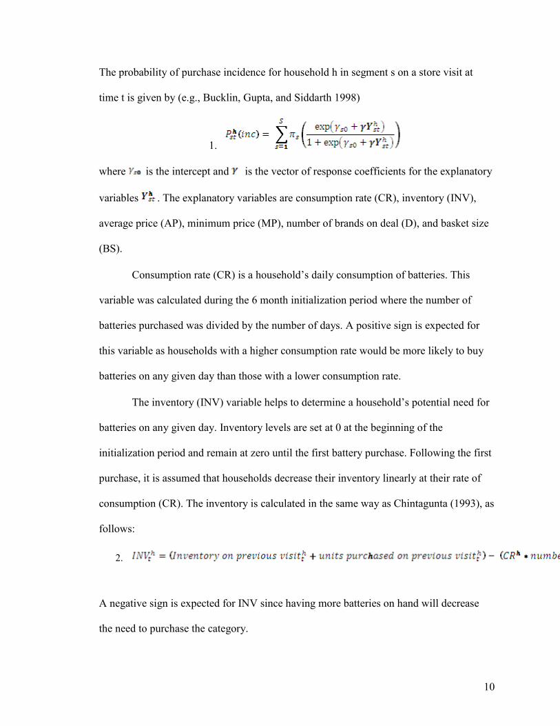
The probability of purchase incidence for household h in segment s on a store visit at
time t is given by (e.g., Bucklin, Gupta, and Siddarth 1998)
1.
where is the intercept and is the vector of response coefficients for the explanatory
variables . The explanatory variables are consumption rate (CR), inventory (INV),
average price (AP), minimum price (MP), number of brands on deal (D), and basket size
(BS).
Consumption rate (CR) is a household’s daily consumption of batteries. This
variable was calculated during the 6 month initialization period where the number of
batteries purchased was divided by the number of days. A positive sign is expected for
this variable as households with a higher consumption rate would be more likely to buy
batteries on any given day than those with a lower consumption rate.
The inventory (INV) variable helps to determine a household’s potential need for
batteries on any given day. Inventory levels are set at 0 at the beginning of the
initialization period and remain at zero until the first battery purchase. Following the first
purchase, it is assumed that households decrease their inventory linearly at their rate of
consumption (CR). The inventory is calculated in the same way as Chintagunta (1993), as
follows:
2.
A negative sign is expected for INV since having more batteries on hand will decrease
the need to purchase the category.
11
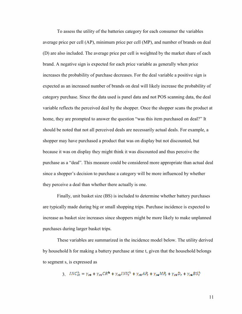
To assess the utility of the batteries category for each consumer the variables
average price per cell (AP), minimum price per cell (MP), and number of brands on deal
(D) are also included. The average price per cell is weighted by the market share of each
brand. A negative sign is expected for each price variable as generally when price
increases the probability of purchase decreases. For the deal variable a positive sign is
expected as an increased number of brands on deal will likely increase the probability of
category purchase. Since the data used is panel data and not POS scanning data, the deal
variable reflects the perceived deal by the shopper. Once the shopper scans the product at
home, they are prompted to answer the question “was this item purchased on deal?” It
should be noted that not all perceived deals are necessarily actual deals. For example, a
shopper may have purchased a product that was on display but not discounted, but
because it was on display they might think it was discounted and thus perceive the
purchase as a “deal”. This measure could be considered more appropriate than actual deal
since a shopper’s decision to purchase a category will be more influenced by whether
they perceive a deal than whether there actually is one.
Finally, unit basket size (BS) is included to determine whether battery purchases
are typically made during big or small shopping trips. Purchase incidence is expected to
increase as basket size increases since shoppers might be more likely to make unplanned
purchases during larger basket trips.
These variables are summarized in the incidence model below. The utility derived
by household h for making a battery purchase at time t, given that the household belongs
to segment s, is expressed as
3.
12
Quantity Model
In the quantity model, the dependent variable is assumed to have a poisson
distribution since purchase occasions typically include only a small number of unit
purchases. Consequently, poisson regression analysis is used. Given that a purchase was
made at time t and that brand i was chosen, the probability that household h buys =
1, 2… n battery cells can be written as (e.g., Bucklin, Gupta, and Siddarth 1998)
4.
where is the purchase rate of household h in segment s for brand i at time t.
To estimate purchase quantity in the batteries category, the variables purchase rate
(PR), inventory (INV), brand loyalty (BL), price (P), brand deal (BD), and basket size
(BS) are included.
Purchase rate (PR) is a household’s average quantity of batteries bought per
purchase occasion. This variable was calculated using the six month initialization period
where the number of batteries purchased was divided by the number of purchase
occasions. A positive sign is expected for this variable as households with a higher
purchase rate would be more likely to buy a larger number of batteries on any given
purchase occasion.
The inventory (INV) variable is the same as defined in the incidence model. A
negative sign is expected for INV since having more batteries on hand will likely
decrease the amount of batteries purchased.
Brand loyalty (BL) is the dollar share of each brand within each individual
household. While Bucklin, Gupta, and Siddarth (1998) calculated each brand’s share
13
during the initialization period and kept this share constant throughout the analysis
period, the brand loyalty variable in this study changes as new purchases are made. A
positive sign is expected for this variable as a stronger brand loyalty towards the
purchased brand would likely lead to a higher number of batteries purchased.
Price (P) refers to the price per cell of the battery purchased at the time of
purchase. A negative sign is expected for this variable as a higher price per cell will
likely lead to fewer battery cells purchased. Brand deal (BD) is a dummy variable with
value = 1 if the buyer perceived there to be a deal during that day for the purchased brand
and value = 0 if the buyer did not perceive there to be a deal. A positive sign is expected
for this variable as the perception of a deal might push the shopper to purchase a higher
quantity of batteries.
Similarly to the incidence model, unit basket size (BS) is included to determine
whether the quantity purchased changes depending on the size of the shopping basket.
Quantity is expected to increase as basket size increases as large basket shoppers will
likely tend to stockpile more than small basket shoppers so they may want to stockpile on
batteries as well, especially since it is a non-perishable and easily storable product.
These variables are summarized in the quantity model below. The poisson rate
parameter for brand i and household h belonging to segment s at time t, is
5.
Analysis Results
Incidence model results
The minimum AIC for the incidence model was not reached at four classes,
however declines in the AIC were minimal for the five segment model and onwards (see
14
table 3 in appendix) so the four class segmentation is used for this analysis. The first class
represents 35% of respondents, the second class 29%, the third class 24%, and the fourth
represents the remaining 11%. Parameter results are shown in the appendix (table 4). The
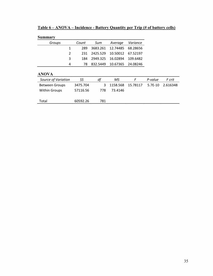
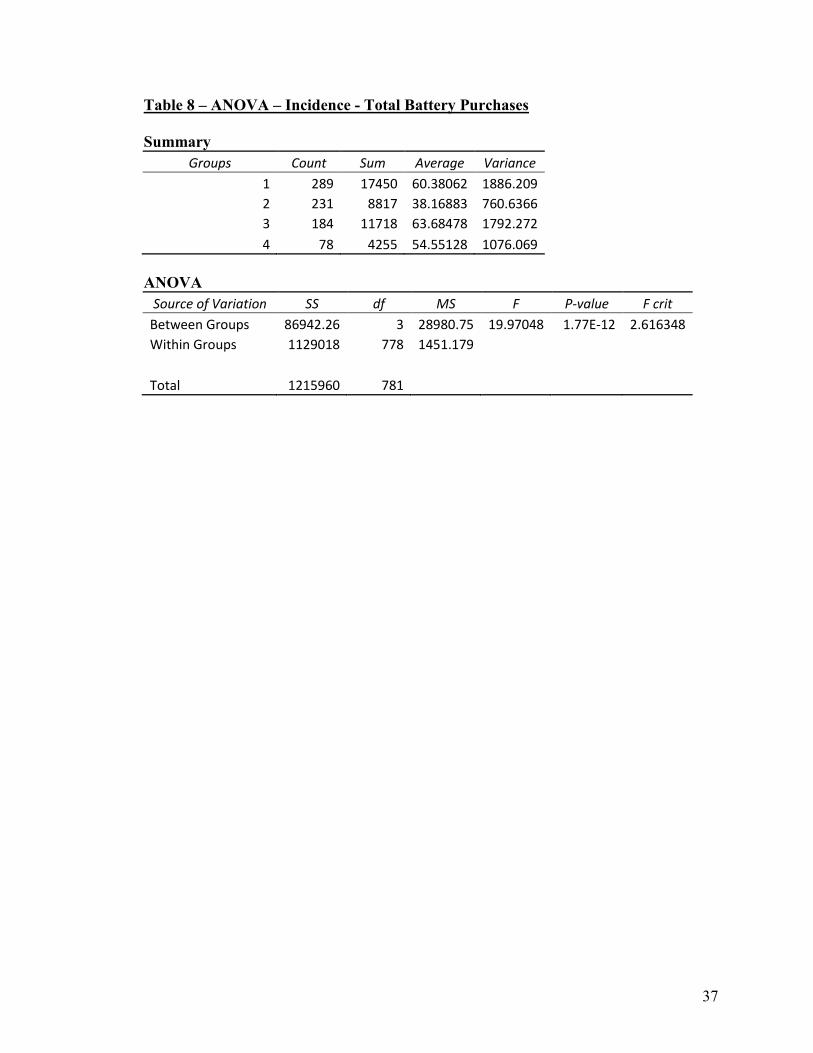
differences between classes were significant for the following variables: male head of
household work hours, battery quantity per trip, battery trip frequency, total battery
purchases, and total trip frequency (See tables 5,6,7,8, and 9 in appendix for ANOVA
results).
The parameters for consumption rate are significant for classes two and three but
they are not in the hypothesized direction; as the consumption rate decreases the
probability of buying in the category increases. This relationship can be explained in two
ways. First, some of these shoppers might be households that have a high usage of
batteries but buy high quantities of batteries per shopping trip, thus needing to do fewer
shopping trips for this category. Second, some consumers may have a low consumption
rate but buy very small quantities per trip and thus run low on inventory quickly.
However, a more likely explanation is the long purchase cycle of batteries and the short
time frame available for this analysis; panelists who bought a larger quantity of batteries
during the initialization period may not have needed to buy as many in the following
twelve month period used for the analysis. This will be discussed further in the
limitations section of this paper.
The inventory parameter estimates for each of the four classes are significant and
in the hypothesized direction; as inventory decreases the probability of buying in the
category increases. Inventory impacts purchase decision most for classes one and three
and least for classes two and four. A weaker influence of inventory for certain consumers
15
is likely due to the fact that batteries are a non-perishable and easily storable product, so
even if inventory is not completely depleted consumers can purchase the category and
store any surplus for future use.
The parameter estimates for minimum price are significant for segments two and
four and in the hypothesized direction; purchase incidence increases as the minimum
price available decreases. This does not necessarily indicate that these shoppers buy the
lowest priced brand, but rather that they are increasingly attracted to the category as the
lowest available price decreases.
The weighted average price significantly impacts all four consumer segments.
Interestingly, the parameters for the first two classes are not in the hypothesized
direction; as the average price increases, purchase incidence increases as well. A possible
explanation is that these households prefer the more expensive brands or the more
expensive chemical types such as lithium and rechargeable, so when there is a good
selection of these more premium products they are more drawn to the category. The third
and fourth classes have the expected negative correlation for this variable.
The deal parameters are significant for the first three classes and in the
hypothesized direction; as the number of brands on deal increases so does the probability
of buying the category. The fourth segment is not influenced by deal activity.
Finally, purchases are more likely during larger basket trips for all four classes of
households. This supports hypothesis 1 and fits with Kollat and Willett (1967) and Park,
Iyer, and Smith’s (1989) findings that unplanned purchases increase as the basket size
increases. As batteries are not a product that is typically purchased weekly, larger (and
16
thus longer) basket trips gives shoppers more time to make unplanned purchases in this
category.
The first class of households is the second highest in terms of overall battery
purchases. These households make the lowest number of shopping trips overall, perhaps
in an effort to save time since the male heads of household work the most hours of all
segments. This group is increasingly likely to buy the category as the average weighted
price increases, indicating that they may have a preference for more expensive chemical
types which last longer and allow them to reduce purchase frequency. Despite their busy
lifestyle, the probability that these households take the time purchase the batteries
category can be increased through promotional activity.
Households in the second segment are not the prime targets for battery
manufacturers and retailers as they are the households that buy the least amount of
batteries. However, these households make the highest number of store visits which
indicates an opportunity to increase purchase incidence of the batteries category. The
probability of a battery purchase can be increased through promotions and pricing.
Interestingly, they are increasingly drawn to the category as the minimum price
decreases, but also as the average price increases. This may indicate that, despite being
price conscious, these shoppers have an interest for premium brands or chemical types.
The third segment of households should be the top priority for manufacturers and
retailers in the batteries category as they are the heaviest purchasers of batteries. Likely
due to their high need for batteries, their probability of purchasing the category increases
more than other household segments in response to average price decreases and
17
promotional increases. Their sensitivity to price and promotion makes them the ideal
targets for marketing activities.
The fourth segment is the least influenced by inventory and at the same time the
most influenced by minimum price and the second most influenced by average price. In
light of this, it is likely that these households take advantage of good prices when they
see them and do not necessarily wait until they need new batteries. The male head of
household tends to work fewer hours than the average which gives them more time to
search for these lower prices.
Quantity model results
The AIC is not minimized at five classes, but in the six class model and onwards
some of the classes are extremely small so the five class model is chosen (See table 10 in
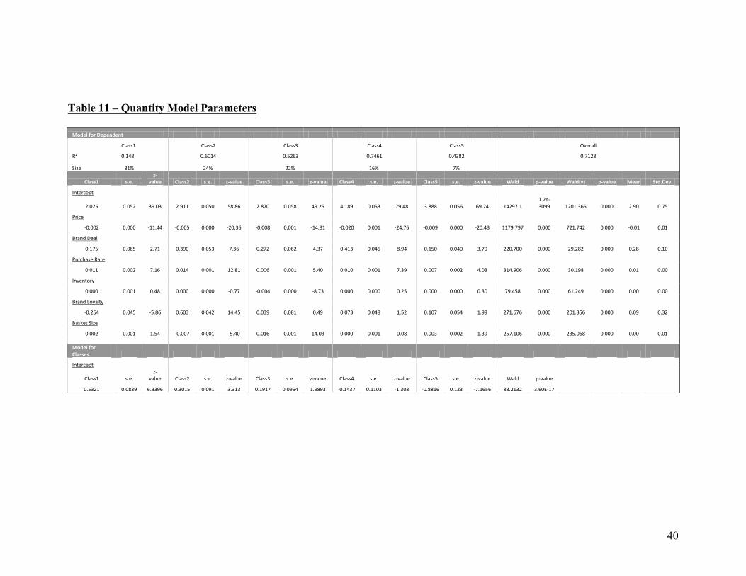
appendix). The first class represents 31% of respondents, the second class 24%, the third
22%, the fourth 16%, and fifth class represents the remaining 7%. The parameter values
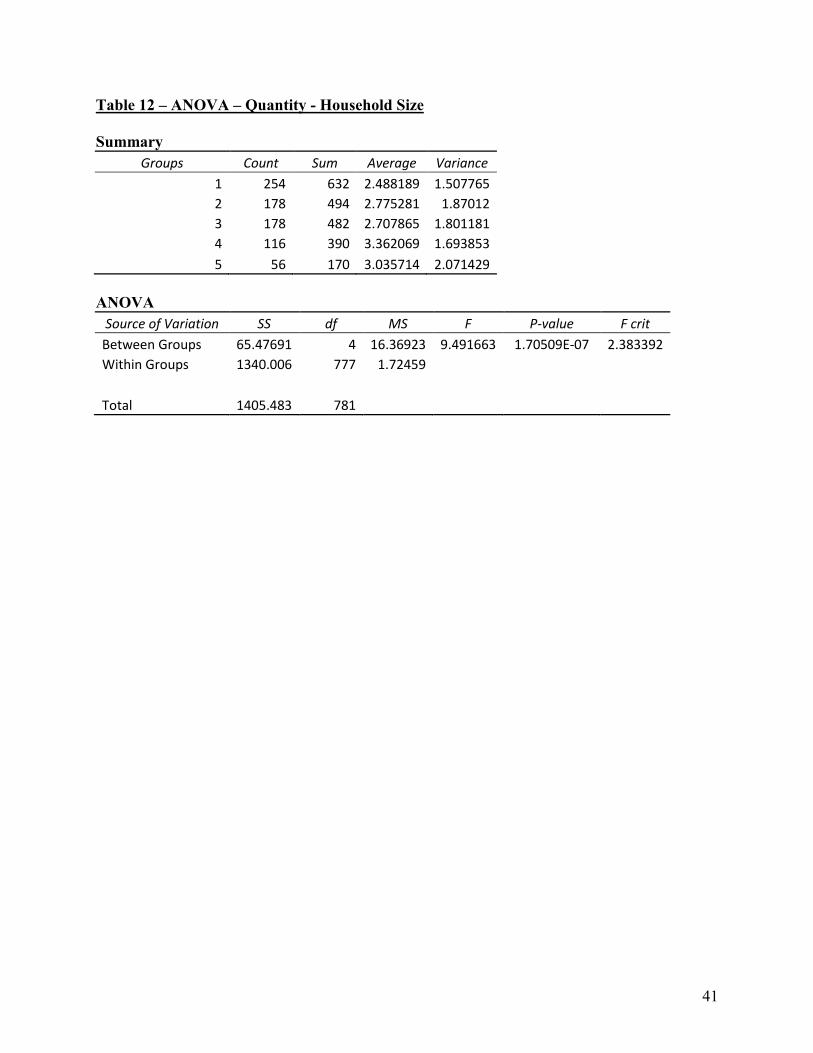
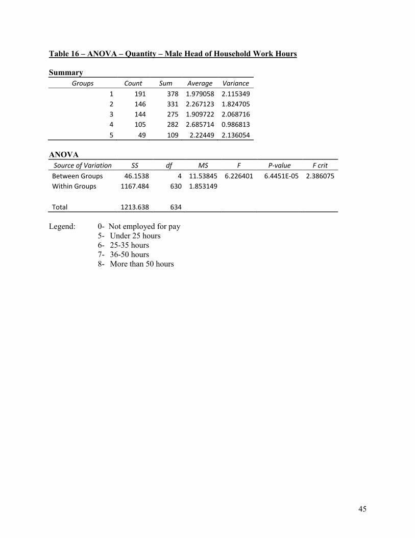
are shown in the appendix (Table 11). All demographic variables are significantly
different between segments except for female head of household education and work
hours (See tables 12 to 21 in appendix).
For each of the five classes of households, the relationship between price and
quantity is significant and in the expected direction. This indicates that battery buyers
will increase their purchase quantity as the price per cell of the brand they are purchasing
decreases.
The relationship with deal is significant and in the expected direction for each of
the five segments. For all classes of households, the quantity of batteries purchased
increases when the buyer perceives there to be a deal on the purchased brand.
18
The purchase rate parameters are significant and in the hypothesized direction for
each of the five segments. This relationship indicates that if a household usually
purchases a large amount of batteries per trip, then they have a higher probability of
buying a larger amount and vice versa.
Only the inventory parameter for the third class is significant and it is in the
hypothesized direction; these buyers are increasingly likely to purchase a larger quantity
as their inventory decreases. The lack of significance of inventory for the other classes
could be because batteries are a non-perishable product so having a higher inventory is
okay because the product will not go to waste. Furthermore, batteries are not very big so
shoppers might be more likely to stockpile in this category than in others where products
are bigger in size and more difficult to store.
The relationship between brand loyalty and purchase quantity is significant for
classes one, two, and five. The parameters are in the hypothesized direction for classes
two and five; when they are purchasing their favorite brand they tend to purchase a
higher number of batteries. However, the first segment’s quantity of purchase decreases
as the brand loyalty of the purchased brand increases. One potential explanation for this
relationship is that these households enjoy trying new things and the lack of excitement
that they get from buying a product that they are familiar with causes them to buy a lower
quantity.
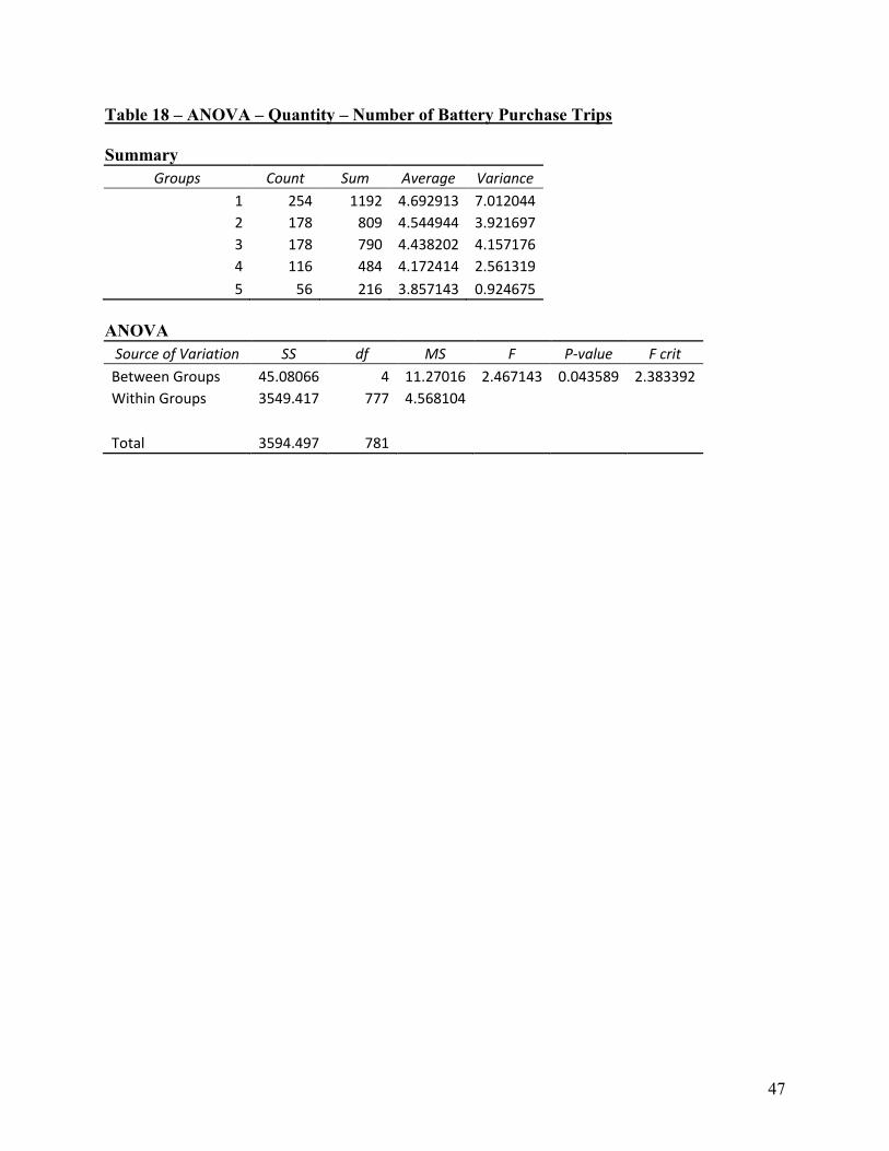
Finally, two of the five parameters for basket size are significant. The third
segment of households buy higher quantities of batteries during larger shopping trips as
predicted. The more time they have during longer trips likely gives them enough time to
evaluate the benefits of buying a larger quantity. However, the second segment buys
19
higher quantities during smaller shopping trips. This could be because when they are
already buying a large basket they try to save money where they can, and thus chose to
buy a smaller amount of batteries.
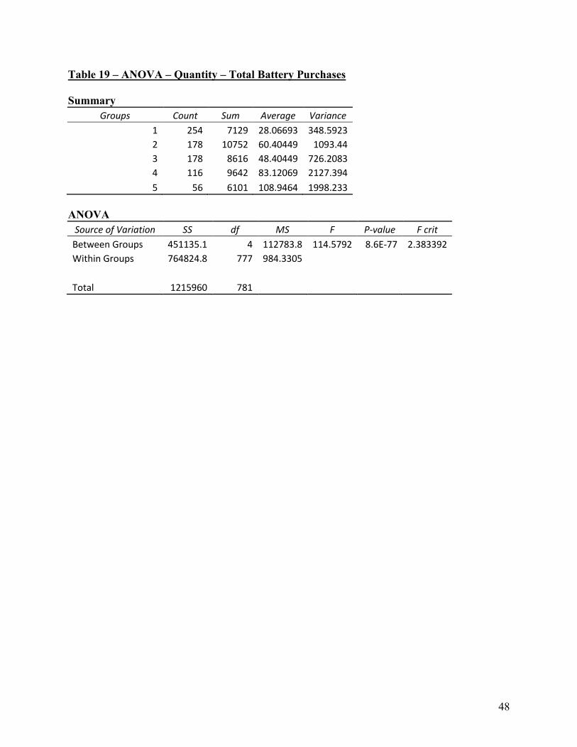
Households in the first class are those who buy the least amount of batteries.
Their lower need for batteries can be explained by the fact that they are the least likely to
have children and thus have the smallest household size. Interestingly, they make the
highest number of battery shopping trips, but their overall battery purchases are brought
down by their very low quantity purchased per trip. A lower price and a perceived deal
on the purchased brand can help to increase purchase quantity, but less so than for most
of the other household segments. Their income is also the lowest of the five segments,
but the fewer household members to support might explain why these households are
among the least sensitive to price and deal. Finally, this segment is the only one to have
an inverse relationship with brand loyalty, so these shoppers prefer buying a larger
quantity when they are buying an unfamiliar brand.
In contrast to the first segment, households in the second segment are the most
brand loyal; purchase quantity increases when the purchased brand is a favored one. They
are also the second most influenced by perceived deal, so promotions can have a positive
impact on the quantity purchased. These households are the only ones who increase their
quantity purchased during smaller shopping trips. In terms of demographic factors these
households have an average household size, an average probability of children, and an
average income. They are overall average buyers of the batteries category.
The third segment ranks fourth out of the five segments in terms of battery
consumption, likely because they also rank fourth in family size. This segment is the only
20
one impacted by inventory; however, inventory is not the only driver of purchase quantity
as these households also respond positively to lower prices and deals. They are the only
households who increase purchase quantity as their basket size increases.
Despite having the second highest income level, households in the fourth segment
are the best target for promotions as they increase quantity purchased the most for a low
price or a deal. This is likely because these households have the biggest families; despite
a higher income, more members to support means having to be more careful with
spending. These households rank second in terms of battery purchases, driven by a high
quantity of batteries per trip which makes up for the fewer than average battery purchase
trips that they make.
Finally, households in the fifth segment have the highest battery purchases overall
likely due to the fact that they have the second largest families. They are the least
responsive to deals, perhaps due to their high income level, however, these households
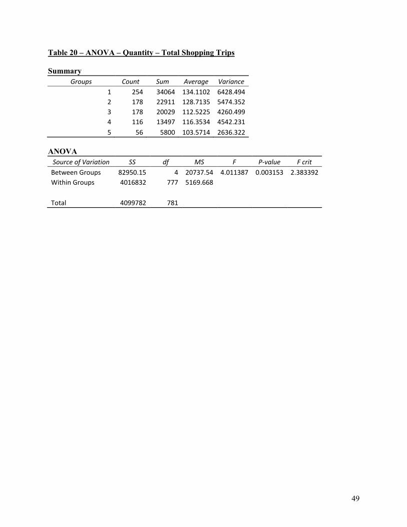
rank second in terms of price sensitivity. Interestingly, they make the least number of
shopping trips overall as well as the least number of battery shopping trips. The fewer
number of trips provides less opportunity to make contact in store so it is important that
retailers offer the right price at the right time to optimize purchase quantity for these
households.
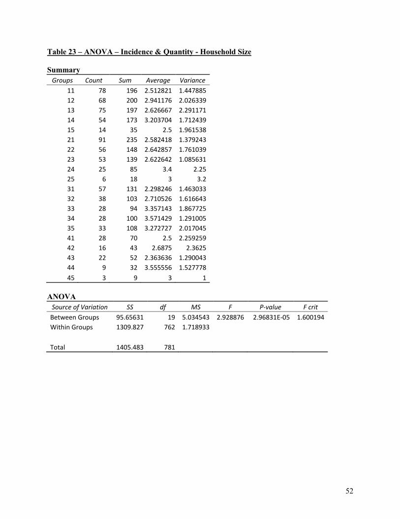
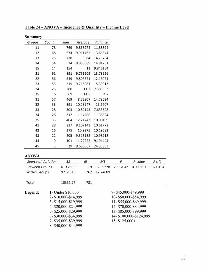
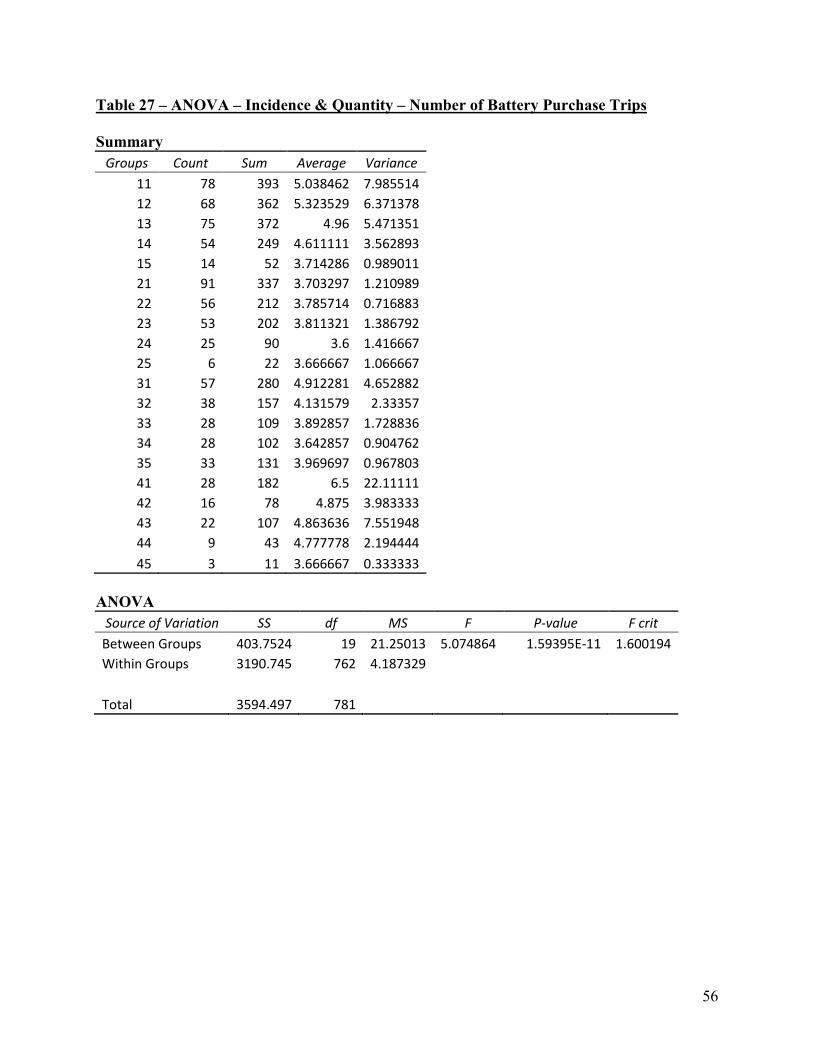
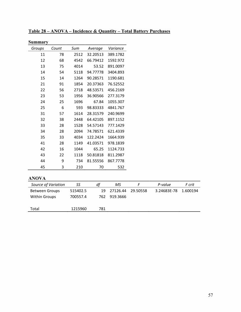
Incidence & Quantity
Combining the incidence and quantity classifications results in 20 different
household segments (4 incidence segments x 5 quantity segments). The six biggest
segments, which together represent 54.3% of households, are described below (see
appendix, table 22, for percentage of households in each segment). There is a significant
21
difference between these segments for all demographic variables except female head of
household education and work hours and male head of household education (see
appendix tables 23 to 30 for ANOVA results).
The biggest segment is households that belong to the second incidence segment
and the first quantity segment; they represent 11.6% of all households. Shoppers in this
segment are the lightest buyers of batteries but they make the most shopping trips overall;
this provides many points of contact with the shopper so there is an opportunity for
retailers and manufacturers to increase purchase incidence of the batteries category.
Promotion and pricing can be used to increase purchase incidence for these buyers as
well as a good assortment of premium products. A competitive price and a deal can help
to increase purchase quantity per trip.
The second largest segment includes households that belong to the first incidence
segment and the first quantity segment; they represent 10% of all households. These
shoppers make more trips for batteries than the average shopper, but their lower quantity
per trip results in an under-average overall purchase quantity. However, purchase
quantity per trip could be increased with promotions and competitive pricing.
Furthermore, purchase incidence could be increased with the use of promotions and a
good assortment of premium battery products.
The third segment includes households that belong to the first incidence segment
and the third quantity segment; they represent 9.6% of all households. Purchase incidence
for these households can be increased with promotions and a good assortment of
premium brands. For this segment of shoppers, both purchase incidence and quantity can
be increased by displaying battery products near items typically bought during larger
22
basket trips. Quantity purchased per trip can also be increased through competitive
pricing and promotions.
The fourth segment includes households that are in the first incidence segment
and the second quantity segment; they represent 8.7% of all households. These
households purchase a higher than average overall quantity of batteries driven by a very
high number of battery shopping trips. While purchase incidence is already high for these
households, it can be further increased through deals as well as a good assortment of
premium brands. These shoppers are the most brand loyal so having the right assortment
of the top brands in the category can help to increase purchase quantity. Furthermore, a
good deal and a competitive price will also help to increase the quantity purchased.
The fifth group includes households from the third incidence segment and the first
quantity segment; they represent 7.3% of all households. These households are some of
the lowest purchasers of batteries due to an extremely low quantity of batteries purchased
per trip. To increase the quantity purchased per trip by these shoppers promotional
activity and a competitive price can be used. Furthermore, as this segment is the most
deal sensitive in their purchase incidence decision, the probability of purchasing for these
shoppers can be increased by offering good promotions. Finally, lowering the average
price per cell in the category can help to drive purchase incidence as well.
Finally, the sixth segment includes households from the second incidence
segment and the second quantity segment; they represent 7.2% of all households. The
goal for this group should be to increase purchase incidence of the batteries category as
these households make a very high number of shopping trips overall but a low number of
battery shopping trips. Purchase incidence for batteries can be increased through
23
promotion as well as a competitive lowest price option. However, a good assortment of
premium brands and positioning next to products typically purchased during large basket
trips can also help to drive incidence.
Summary and Discussion
Perceived deal was found to positively influence purchase incidence in 89% of
consumers and purchase quantity in 100% of consumers. This highlights the importance
of promotional activity in the batteries category. Analysts can use retailer POS scanning
data to determine the percentage of volume actually sold on deal and compare this to the
percentage sold on perceived deal through Nielsen’s Homescan panel. This will
determine whether shoppers are realizing that they are buying on deal, or whether the
promotions are being done in vain. If perceived deal is found to be much lower than
actual volume sold on deal, promotional activity should be modified until the two
measures show similar results. It is important to determine what is perceived as a good
deal by consumers. For some battery buyers, a perceived deal might not be the result of a
low price, but rather might be the result of a reasonable price for a favored brand. In this
post-recession environment consumers are still being cautious in their spending, but they
are responding to good value (The Nielsen Company, 2010). Retailers and manufacturers
must determine what shoppers see as good value in the batteries category.
The incidence model showed that 40% of households increased their likelihood of
buying the category as the minimum price decreased. This result shows that, while a low
price is important for some consumers, an even higher percentage of shoppers will not be
increasingly drawn to the category by a low price point. To further strengthen this
argument, an even higher percentage of households (65%) were increasingly likely to
24
purchase the category as the average price increased. This indicates that retailers should
have a strong assortment of premium battery products to help attract shoppers to the
category. However, a competitive price is still important as all consumers were found to
increase the quantity purchased as the price per cell of the purchased brand decreased.
Finally, increases in basket size were found to positively impact purchase
incidence for 100% of households and purchase quantity for 37% of households. This is a
very interesting finding for both manufacturers and retailers who compete in the batteries
category. To help increase battery purchase incidence and quantity, displays for batteries
should be placed close to products that are typically purchased during large basket
shopping trips.
Limitations and Future Research
The first limitation of this paper is that joint estimation was not done. As Bucklin,
Gupta, and Siddarth (1998) found, results can differ between separate estimation and
joint estimation procedures. Since the purchase incidence and purchase quantity
decisions are made simultaneously by shoppers, modeling these consumer responses
together may have resulted in more significant findings.
Another important decision made by shoppers is their brand choice and this would
be an interesting area of research for future studies. Results from a brand choice study
would be useful for manufacturers of the batteries category as they could benefit from
insights into ways of increasing the probability that their brands are chosen by
consumers. Retailers would also benefit since they could use results to increase sales for
their private label battery products.
25
A third limitation is the low pseudo R2 of approximately 7% for the incidence
model. This indicates that there are important variables that may not have been included
in the model. Chintagunta (1993) found that the larger the brand, the greater impact its
marketing variables have on purchase incidence. Given this result, including a brand
share measure in the incidence model could help improve the model’s pseudo R2.
Another variable that could be added to the incidence model is store loyalty. As Kahn and
Schmittlein (1992) claim, larger shopping trips typically occur at a shopper’s favorite
store. Since basket size was found to increase purchase incidence for all battery buyers in
this study, it is possible that the larger basket purchases done in favored stores would
drive higher purchase incidence. However, Kahn and Schmittlein (1992) also suggest the
possibility that consumers might be more open to non-planned purchases when they are
outside of their regular routine, thus in a non-favorite store. This suggests that store
loyalty could have a negative impact on purchase incidence. Further research could
determine which (if any) assumption is correct by determining if store loyalty impacts
purchase incidence. Store format could also have been included in the purchase incidence
model. Retail banners such as Costco and Wal-Mart typically experience larger basket
sales, so shopping in these retailers could positively influence the likelihood of purchase
in the batteries category. Furthermore, the number of categories in the shopping basket
might impact the purchase incidence decision since buying many different categories
suggests that shoppers walked through more aisles in the store, increasing the probability
of walking past the batteries category and making a purchase.
Another factor that may have negatively impacted the incidence model is the long
purchase cycle of the batteries category; this category is not one that is purchased
26
frequently by many households. While only households that did at least three purchases
during the twelve month estimation period were included in the study, this may not be
enough. This might also explain why the consumption rate variable was negatively
correlated with purchase incidence. It is possible that the consumers who purchased more
batteries in the initialization period needed to buy less in the twelve month period that
followed. Having a longer period of data may have improved the significance of this
variable.
The method in which the deal variable is recorded in the data retrieval process
could also be considered a limitation. All that is known from this variable is that the
shopper perceived the purchase to be on deal but the type of promotion (if any) is
unknown. The promotion could be a flyer ad, a display, a coupon, or simply a price
reduction in store. Knowing these additional facts would help to narrow down the
influence that promotions have on incidence and quantity and would help to determine
which types of promotions should be used for the various household segments. Having
this level of detail may also have improved the pseudo R2
of the incidence model.
A final limitation is that only one product category was studied so the results do
not necessarily apply to all other categories. There would probably be significant
differences for product categories that are not easily storable as inventory would likely
play a much more significant role in both purchase incidence and purchase quantity
decisions. Future studies could focus within non-perishable products and segment
product categories by size as consumers should be more likely to stockpile smaller
products.
27
References
Andrews, Rick L., Asim Ansari, & Imran S. Currim (2002), “Hierarchical Bayes versus
Finite Mixture Conjoint Analysis Models: A Comparison of Fit, Prediction, and
Partworth Recovery,” Journal of Marketing Research, 39 (February), 87-98.
Bell, David R., Jeongwen Chiang, & V. Padmanabhan (1999). “The Decomposition of
Promotional Response: An Empirical Generalization,” Marketing Science, 18(4),
504-26.
Bucklin, Randolph E. and Sunil Gupta (1992), “Brand Choice, Purchase Incidence, and
Segmentation: An Integrated Approach,” Journal of Marketing Research, 29
(May), 201-15.
Bucklin, Randolph E., Sunil Gupta, and S. Siddarth (1998), “Determining Segmentation
in Sales Response across Consumer Purchase Behaviors,” Journal of Marketing
Research, 35 (May), 189-97.
Chiang, Jeongwen (1991), “A Simultaneous Approach to the Whether, What and How
Much to Buy Questions,” Marketing Science (1986-1998), 10(4), 297.
Chintagunta, Pradeep K. (1993). Investigating Purchase Incidence, Brand Choice and
Purchase Quantity Decisions of Households. Marketing Science (1986-
1998), 12(2), 184.
Gupta, Sunil (1988), “Impact of Sales Promotions on When, What, and How Much to
Buy,” Journal of Marketing Research, 25 (November), 342-55.
Kahn, Barbara E., and David C. Schmittlein (1992), “The Relationship Between
Purchases Made on Promotion and Shopping Trip Behavior,” Journal of
Retailing, 68 (3), 294-315.
28
Kamakura, Wagner A., and Gary J. Russell (1989), “A Probabilistic Choice Model for
Market Segmentation and Elasticity Structure,” Journal of Marketing Research,
26 (November), 379-90.
Kollat, David T., and Ronald P. Willett (1967), “Customer Impulse Purchasing
Behavior,” Journal of Marketing Research, IV (February), 21-31.
Neslin, Scott, Caroline Henderson, and John Quelch (1985), “Consumer Promotions and
the Acceleration of Product Purchases,” Marketing Science, 4 (spring), 147-65.
Park, C. Whan, Easwar S. Iyer, and Daniel C. Smith (1989), “The Effects of Situational
Factors on In-Store Grocery Shopping Behavior: The Role of Store Environment
and Time Available for Shopping,” Journal of Consumer Research, 15 (March),
422-33.
The Nielsen Company (2010), “Canadian Confidence Leading the Pace…but Consumer
Restraint Becomes the New Normal: A Canadian Perspective.” Retrieved
November 9, 2010, from http://en-
ca.nielsen.com/content/dam/nielsen/en_ca/documents/pdf/reports/Consumer%20
Confidence%20-%20Canadian%20Perspective%20-%20May%202010.pdf
The Nielsen Company (2009), “Global Consumer Confidence Rebounding, and Sales
Start to Follow,” Nielsen Wire, (November 30). Retrieved November 2, 2010,
from http://blog.nielsen.com/nielsenwire/consumer/global-consumer-confidence-
rebounding-and-sales-start-to-follow/
The Nielsen Company (2010), “Nielsen Economic Current Q2 2010: The State of the
Global Consumer,” Nielsen Wire, (July 20). Retrieved November 7, 2010, from
29
http://blog.nielsen.com/nielsenwire/consumer/nielsen-economic-current-q2-2010-
the-state-of-the-global-consumer/
The Nielsen Company (2010), “Global Consumer Strategies for Saving Money,” Nielsen
Wire, (September 2). Retrieved November 2, 2010, from
http://blog.nielsen.com/nielsenwire/consumer/global-consumer-strategies-for-
saving-money/
30
Appendices
Table 1 – Brand Shares
Brand Indicator Brand Chemical Cell Size Shr Cum Shr
1 A A AA 23.9 23.9
2 B A AA 12.6 36.5
3 A A AAA 12.4 48.9
4 B A AAA 8.7 57.5
5 B B AA 4.3 61.8
6 B C AA 2.9 64.7
7 A B AA 2.8 67.5
8 C A AA 2.3 69.8
9 D A AAA 2.0 71.8
10 E A AA 1.9 73.6
11 D A AA 1.8 75.5
12 C A AAA 1.8 77.2
13 F A AAA 1.7 78.9
14 B B AAA 1.7 80.6
31
Table 2 – Outlet Shares
Outlet Outlet Share Cum Shr
Wal-Mart 19.2 19.2 Price/Costco 17.2 36.5 Canadian Tire 8.0 44.5
Real Canadian Superstore West 4.9 49.4 Zellers 4.9 54.3
Shoppers Drug Mart 4.9 59.2 Safeway 2.5 61.7
Jean Coutu 1.9 63.6 Atlantic Superstore 1.6 65.2
Dollarama 1.6 66.8 Wal-Mart Supercentre 1.6 68.4
All Other Stores 1.5 69.9 London Drugs 1.5 71.3
Sobeys 1.4 72.8 Loblaws 1.3 74.1
Home Hardware 1.3 75.4 Business Depot/Staples/Bureau En Gros 1.1 76.4
Zehrs 0.9 77.3 Pharma Plus 0.9 78.2
Real Canadian Superstore 0.8 79.0 Extra Foods 0.8 79.8
Future Shop 0.8 80.6
32
Table 3 – Incidence Model AICs
Classes AIC Difference 1 28411 2 27846 565 3 27608 238 4 27480 128 5 27420 60 6 27362 58 7 27330 32 8 27314 16 9 27287 27
10 27302 -15
33
Table 4 – Incidence Parameters
Model for Dependent
Class1 Class2 Class3 Class4 Overall
R² 0.0367 0.0111 0.0938 0.1417 0.0717
Size 35% 29% 24% 11%
Class1 s.e. z-value Class2 s.e. z-value Class3 s.e. z-value Class4 s.e. z-value Wald p-value Wald(=) p-value Mean Std.Dev.
Intercept
-4.041 0.300 -13.479 -2.840 0.313 -9.068 -0.549 0.186 -2.954 2.6376 0.3632 7.261 475.0062 1.70E-101 352.1357 5.10E-76 -2.0974 2.1416
Basket Size
0.046 0.003 16.118 0.029 0.003 10.208 0.042 0.003 12.148 0.0496 0.0074 6.7447 776.4317 9.80E-167 20.3711 0.00014 0.0408 0.0076
Consumption Rate
-0.300 0.247 -1.217 -1.342 0.472 -2.841 -1.276 0.330 -3.871 -1.165 0.7434 -1.5673 29.4819 6.20E-06 8.4846 0.037 -0.938 0.4744
Inventory
-0.013 0.002 -8.652 -0.010 0.002 -4.074 -0.012 0.002 -7.160 -0.009 0.0036 -2.4403 192.627 1.40E-40 2.2354 0.52 -0.0114 0.0018
Minimum Price
-0.002 0.002 -0.922 -0.040 0.005 -7.780 0.002 0.003 0.646 -0.0966 0.0088 -11 217.4671 6.60E-46 213.5436 5.00E-46 -0.023 0.0316
Average Price
0.005 0.002 3.042 0.006 0.002 2.859 -0.035 0.002 -15.251 -0.0164 0.0022 -7.7186 466.8141 1.00E-99 461.5828 1.00E-99 -0.0066 0.0172
Deal Count
0.479 0.044 10.969 0.175 0.062 2.812 0.633 0.058 10.997 -0.0066 0.1168 -0.0559 322.4782 1.50E-68 47.7074 2.50E-10 0.373 0.219
Model for Classes
Intercept
Class1 s.e. z-value Class2 s.e. z-value Class3 s.e. z-value Class4 s.e. z-value Wald p-value
0.4297 0.1148 3.7427 0.2405 0.1295 1.8563 0.0503 0.1165 0.4313 -0.7204 0.1671 -4.3107 24.9703 1.60E-05
34
Table 5 – ANOVA – Incidence - Male Head of Household Work Hours
Summary
Groups Count Sum Average Variance
1 232 565 2.435345 1.519611 2 195 399 2.046154 2.033941 3 148 304 2.054054 2.119507
4 60 107 1.783333 2.138701
ANOVA
Source of Variation SS df MS F P-value F crit
Between Groups 30.27211 3 10.0907 5.380613 0.00116 2.619022
Within Groups 1183.366 631 1.875381
Total 1213.638 634
Legend: 0- Not employed for pay
1- Under 25 hours
2- 25-35 hours
3- 36-50 hours
4- More than 50 hours
35
Table 6 – ANOVA – Incidence - Battery Quantity per Trip (# of battery cells)
Summary
Groups Count Sum Average Variance
1 289 3683.261 12.74485 68.28656 2 231 2425.529 10.50012 67.52197 3 184 2949.325 16.02894 109.6482
4 78 832.5449 10.67365 24.08246
ANOVA
Source of Variation SS df MS F P-value F crit
Between Groups 3475.704 3 1158.568 15.78117 5.7E-10 2.616348
Within Groups 57116.56 778 73.4146
Total 60592.26 781
36
Table 7 – ANOVA – Incidence - Number of Battery Purchase Trips
Summary
Groups Count Sum Average Variance
1 289 1428 4.941176 5.854167 2 231 863 3.735931 1.134312 3 184 779 4.233696 2.682793
4 78 421 5.397436 11.56727
ANOVA
Source of Variation SS df MS F P-value F crit
Between Groups 265.9751 3 88.65836 20.72277 6.34E-13 2.616348
Within Groups 3328.522 778 4.278306
Total 3594.497 781
37
Table 8 – ANOVA – Incidence - Total Battery Purchases
Summary
Groups Count Sum Average Variance
1 289 17450 60.38062 1886.209 2 231 8817 38.16883 760.6366 3 184 11718 63.68478 1792.272
4 78 4255 54.55128 1076.069
ANOVA
Source of Variation SS df MS F P-value F crit
Between Groups 86942.26 3 28980.75 19.97048 1.77E-12 2.616348
Within Groups 1129018 778 1451.179
Total 1215960 781
38
Table 9 – ANOVA – Incidence - Number of Total Shopping Trips
Summary
Groups Count Sum Average Variance
1 289 26442 91.49481 3026.508 2 231 37150 160.8225 5659.981 3 184 24440 132.8261 4844.789
4 78 8269 106.0128 4963.493
ANOVA
Source of Variation SS df MS F P-value F crit
Between Groups 657566.7 3 219188.9 49.54047 2.63E-29 2.616348
Within Groups 3442215 778 4424.441
Total 4099782 781
39
Table 10 – Quantity Model AICs
Classes AIC Difference 1 32240 2 25982 6258 3 24717 1265 4 24057 660 5 23756 301 6 23450 306 7 23147 303 8 22961 186
40
Table 11 – Quantity Model Parameters
Model for Dependent
Class1 Class2 Class3 Class4 Class5 Overall
R² 0.148 0.6014 0.5263 0.7461 0.4382 0.7128
Size 31% 24% 22% 16% 7%
Class1 s.e. z-
value Class2 s.e. z-value Class3 s.e. z-value Class4 s.e. z-value Class5 s.e. z-value Wald p-value Wald(=) p-value Mean Std.Dev.
Intercept
2.025 0.052 39.03 2.911 0.050 58.86 2.870 0.058 49.25 4.189 0.053 79.48 3.888 0.056 69.24 14297.1 1.2e-3099 1201.365 0.000 2.90 0.75
Price
-0.002 0.000 -11.44 -0.005 0.000 -20.36 -0.008 0.001 -14.31 -0.020 0.001 -24.76 -0.009 0.000 -20.43 1179.797 0.000 721.742 0.000 -0.01 0.01
Brand Deal
0.175 0.065 2.71 0.390 0.053 7.36 0.272 0.062 4.37 0.413 0.046 8.94 0.150 0.040 3.70 220.700 0.000 29.282 0.000 0.28 0.10
Purchase Rate
0.011 0.002 7.16 0.014 0.001 12.81 0.006 0.001 5.40 0.010 0.001 7.39 0.007 0.002 4.03 314.906 0.000 30.198 0.000 0.01 0.00
Inventory
0.000 0.001 0.48 0.000 0.000 -0.77 -0.004 0.000 -8.73 0.000 0.000 0.25 0.000 0.000 0.30 79.458 0.000 61.249 0.000 0.00 0.00
Brand Loyalty
-0.264 0.045 -5.86 0.603 0.042 14.45 0.039 0.081 0.49 0.073 0.048 1.52 0.107 0.054 1.99 271.676 0.000 201.356 0.000 0.09 0.32
Basket Size
0.002 0.001 1.54 -0.007 0.001 -5.40 0.016 0.001 14.03 0.000 0.001 0.08 0.003 0.002 1.39 257.106 0.000 235.068 0.000 0.00 0.01
Model for Classes
Intercept
Class1 s.e. z-
value Class2 s.e. z-value Class3 s.e. z-value Class4 s.e. z-value Class5 s.e. z-value Wald p-value
0.5321 0.0839 6.3396 0.3015 0.091 3.313 0.1917 0.0964 1.9893 -0.1437 0.1103 -1.303 -0.8816 0.123 -7.1656 83.2132 3.60E-17
41
Table 12 – ANOVA – Quantity - Household Size
Summary
Groups Count Sum Average Variance
1 254 632 2.488189 1.507765 2 178 494 2.775281 1.87012 3 178 482 2.707865 1.801181 4 116 390 3.362069 1.693853
5 56 170 3.035714 2.071429
ANOVA
Source of Variation SS df MS F P-value F crit
Between Groups 65.47691 4 16.36923 9.491663 1.70509E-07 2.383392 Within Groups 1340.006 777 1.72459
Total 1405.483 781
42
Table 13 – ANOVA – Quantity – Income Level
Summary
Groups Count Sum Average Variance
1 254 2356 9.275591 13.52849 2 178 1789 10.05056 12.78274 3 178 1761 9.893258 13.35012 4 116 1227 10.57759 12.14175
5 56 656 11.71429 9.98961
ANOVA
Source of Variation SS df MS F P-value F crit
Between Groups 337.8153 4 84.45382 6.566031 3.37E-05 2.383392 Within Groups 9993.956 777 12.86223
Total 10331.77 781
Legend: 1- Under $10,000
2- $10,000-$14,999
3- $15,000-$19,999
4- $20,000-$24,999
5- $25,000-$29,999
6- $30,000-$34,999
7- $35,000-$39,999
8- $40,000-$44,999
9- $45,000-$49,999
10- $50,000-$54,999
11- $55,000-$69,999
12- $70,000-$84,999
13- $85,000-$99,999
14- $100,000-$124,999
15- $125,000+
43
Table 14 – ANOVA – Quantity – Presence of Children
Summary
Groups Count Sum Average Variance
1 254 78 0.307087 0.213625 2 178 69 0.38764 0.238716 3 178 59 0.331461 0.222846 4 116 69 0.594828 0.243103
5 56 24 0.428571 0.249351
ANOVA
Source of Variation SS df MS F P-value F crit
Between Groups 7.261415014 4 1.815354 7.950452 2.78E-06 2.383392 Within Groups 177.4150556 777 0.228333
Total 184.6764706 781
Legend: 0 – No Children
1 - Children
44
Table 15 – ANOVA – Quantity – Male Head of Household Education
Summary
Groups Count Sum Average Variance
1 191 828 4.335079 2.950289 2 146 690 4.726027 3.20718 3 144 621 4.3125 2.593969 4 105 493 4.695238 2.790842
5 49 259 5.285714 2.375
ANOVA
Source of Variation SS df MS F P-value F crit
Between Groups 50.20149 4 12.55037 4.390725 0.001653 2.386075 Within Groups 1800.781 630 2.858383
Total 1850.983 634
Legend: 1- Elementary School
2- Some High School
3- Completed High School
4- Some Technical or College
5- Completed Technical or College
6- Some University
7- Completed University
45
Table 16 – ANOVA – Quantity – Male Head of Household Work Hours
Summary
Groups Count Sum Average Variance
1 191 378 1.979058 2.115349 2 146 331 2.267123 1.824705 3 144 275 1.909722 2.068716 4 105 282 2.685714 0.986813
5 49 109 2.22449 2.136054
ANOVA
Source of Variation SS df MS F P-value F crit
Between Groups 46.1538 4 11.53845 6.226401 6.4451E-05 2.386075 Within Groups 1167.484 630 1.853149
Total 1213.638 634
Legend: 0- Not employed for pay
5- Under 25 hours
6- 25-35 hours
7- 36-50 hours
8- More than 50 hours
46
Table 17 – ANOVA – Quantity – Battery Quantity per Trip (# of battery cells)
Summary
Groups Count Sum Average Variance
1 254 1498.823 5.900878 2.98169 2 178 2414.38 13.56393 34.0639 3 178 1989.246 11.17554 22.32373 4 116 2390.31 20.60612 86.98416
5 56 1597.9 28.53393 114.1283
ANOVA
Source of Variation SS df MS F P-value F crit
Between Groups 33577.05 4 8394.262 241.4322 1.1113E-134 2.383392 Within Groups 27015.22 777 34.76862
Total 60592.26 781
47
Table 18 – ANOVA – Quantity – Number of Battery Purchase Trips
Summary
Groups Count Sum Average Variance
1 254 1192 4.692913 7.012044 2 178 809 4.544944 3.921697 3 178 790 4.438202 4.157176 4 116 484 4.172414 2.561319
5 56 216 3.857143 0.924675
ANOVA
Source of Variation SS df MS F P-value F crit
Between Groups 45.08066 4 11.27016 2.467143 0.043589 2.383392 Within Groups 3549.417 777 4.568104
Total 3594.497 781
48
Table 19 – ANOVA – Quantity – Total Battery Purchases
Summary
Groups Count Sum Average Variance
1 254 7129 28.06693 348.5923 2 178 10752 60.40449 1093.44 3 178 8616 48.40449 726.2083 4 116 9642 83.12069 2127.394
5 56 6101 108.9464 1998.233
ANOVA
Source of Variation SS df MS F P-value F crit
Between Groups 451135.1 4 112783.8 114.5792 8.6E-77 2.383392 Within Groups 764824.8 777 984.3305
Total 1215960 781
49
Table 20 – ANOVA – Quantity – Total Shopping Trips
Summary
Groups Count Sum Average Variance
1 254 34064 134.1102 6428.494 2 178 22911 128.7135 5474.352 3 178 20029 112.5225 4260.499 4 116 13497 116.3534 4542.231
5 56 5800 103.5714 2636.322
ANOVA
Source of Variation SS df MS F P-value F crit
Between Groups 82950.15 4 20737.54 4.011387 0.003153 2.383392 Within Groups 4016832 777 5169.668
Total 4099782 781
50
Table 21 – ANOVA – Quantity – Average Shopping Basket Size
Summary
Groups Count Sum Average Variance
1 254 1975.55 7.777754 24.66951 2 178 1599.243 8.98451 40.66417 3 178 1512.008 8.494429 27.3889 4 116 1240.124 10.69073 47.93752
5 56 457.662 8.172536 21.69965
ANOVA
Source of Variation SS df MS F P-value F crit
Between Groups 712.8024 4 178.2006 5.540009 0.000212 2.383392 Within Groups 24993.08 777 32.16612
Total 25705.88 781
51
Table 22 – Percentage of Households in Each Segment – Incidence & Quantity
Incidence Class Quantity Class % of Households 1 1 10.0 1 2 8.7 1 3 9.6 1 4 6.9 1 5 1.8 2 1 11.6 2 2 7.2 2 3 6.8 2 4 3.2
2 5 0.8 3 1 7.3 3 2 4.9 3 3 3.6 3 4 3.6 3 5 4.2 4 1 3.6 4 2 2.0 4 3 2.8 4 4 1.2 4 5 0.4
52
Table 23 – ANOVA – Incidence & Quantity - Household Size
Summary
Groups Count Sum Average Variance
11 78 196 2.512821 1.447885 12 68 200 2.941176 2.026339 13 75 197 2.626667 2.291171 14 54 173 3.203704 1.712439 15 14 35 2.5 1.961538 21 91 235 2.582418 1.379243 22 56 148 2.642857 1.761039 23 53 139 2.622642 1.085631
24 25 85 3.4 2.25 25 6 18 3 3.2 31 57 131 2.298246 1.463033 32 38 103 2.710526 1.616643 33 28 94 3.357143 1.867725 34 28 100 3.571429 1.291005 35 33 108 3.272727 2.017045 41 28 70 2.5 2.259259 42 16 43 2.6875 2.3625 43 22 52 2.363636 1.290043 44 9 32 3.555556 1.527778
45 3 9 3 1
ANOVA
Source of Variation SS df MS F P-value F crit
Between Groups 95.65631 19 5.034543 2.928876 2.96831E-05 1.600194 Within Groups 1309.827 762 1.718933
Total 1405.483 781
53
Table 24 – ANOVA – Incidence & Quantity – Income Level
Summary
Groups Count Sum Average Variance
11 78 769 9.858974 11.88894 12 68 674 9.911765 13.66374 13 75 738 9.84 14.75784 14 54 534 9.888889 14.81761 15 14 154 11 9.846154 21 91 891 9.791209 13.78926 22 56 549 9.803571 12.16071 23 53 515 9.716981 15.39913
24 25 280 11.2 7.583333 25 6 69 11.5 4.7 31 57 469 8.22807 14.78634 32 38 391 10.28947 13.6707 33 28 303 10.82143 7.633598 34 28 312 11.14286 11.38624 35 33 404 12.24242 10.00189 41 28 227 8.107143 10.61772 42 16 175 10.9375 10.19583 43 22 205 9.318182 10.98918 44 9 101 11.22222 9.194444
45 3 29 9.666667 24.33333
ANOVA
Source of Variation SS df MS F P-value F crit
Between Groups 619.2533 19 32.59228 2.557042 0.000291 1.600194 Within Groups 9712.518 762 12.74609
Total 10331.77 781
Legend: 1- Under $10,000 9- $45,000-$49,999
2- $10,000-$14,999 10- $50,000-$54,999
3- $15,000-$19,999 11- $55,000-$69,999
4- $20,000-$24,999 12- $70,000-$84,999
5- $25,000-$29,999 13- $85,000-$99,999
6- $30,000-$34,999 14- $100,000-$124,999
7- $35,000-$39,999 15- $125,000+
8- $40,000-$44,999
54
Table 25 – ANOVA – Incidence & Quantity – Male Head of Household Work Hours
Summary
Groups Count Sum Average Variance
11 59 142 2.40678 1.659264 12 56 145 2.589286 1.410065 13 57 125 2.192982 1.72995 14 48 128 2.666667 0.907801 15 12 25 2.083333 2.628788 21 75 146 1.946667 2.024144 22 46 93 2.021739 2.110628 23 45 81 1.8 2.3
24 24 66 2.75 0.978261 25 5 13 2.6 2.3 31 38 57 1.5 2.364865 32 30 69 2.3 1.803448 33 25 44 1.76 2.106667 34 25 65 2.6 1.5 35 30 69 2.3 2.07931 41 19 33 1.736842 2.649123 42 14 24 1.714286 2.065934 43 17 25 1.470588 2.389706 44 8 23 2.875 0.125
45 2 2 1 0
ANOVA
Source of Variation SS df MS F P-value F crit
Between Groups 93.40983 19 4.916307 2.69903 0.000134 1.603471 Within Groups 1120.228 615 1.821509
Total 1213.638 634
Legend: 0- Not employed for pay
9- Under 25 hours
10- 25-35 hours
11- 36-50 hours
12- More than 50 hours
55
Table 26 – ANOVA – Incidence & Quantity –Battery Quantity per Trip (# of battery cells)
Summary
Groups Count Sum Average Variance
11 78 496.3662 6.363669 3.547204 12 68 859.9467 12.64628 30.0008 13 75 830.5382 11.07384 19.53411 14 54 1151.276 21.31993 107.473 15 14 345.1333 24.65238 69.21311 21 91 502.4286 5.521193 2.828946 22 56 723.2667 12.91548 25.31992 23 53 522.9095 9.866217 17.25038
24 25 501.7905 20.07162 121.8047 25 6 175.1333 29.18889 614.5394 31 57 326.4222 5.726706 2.590086 32 38 621.0762 16.34411 55.74216 33 28 397.0833 14.18155 38.18311 34 28 583.2762 20.83129 40.75983 35 33 1021.467 30.95354 49.41513 41 28 173.6061 6.200216 1.760018 42 16 210.0905 13.13065 12.44465 43 22 238.715 10.85068 10.99265 44 9 153.9667 17.10741 17.12938
45 3 56.16667 18.72222 13.89815
ANOVA
Source of Variation SS df MS F P-value F crit
Between Groups 35177.36 19 1851.44 55.51064 1.3943E-129 1.600194 Within Groups 25414.9 762 33.35289
Total 60592.26 781
56
Table 27 – ANOVA – Incidence & Quantity – Number of Battery Purchase Trips
Summary
Groups Count Sum Average Variance
11 78 393 5.038462 7.985514 12 68 362 5.323529 6.371378 13 75 372 4.96 5.471351 14 54 249 4.611111 3.562893 15 14 52 3.714286 0.989011 21 91 337 3.703297 1.210989 22 56 212 3.785714 0.716883 23 53 202 3.811321 1.386792
24 25 90 3.6 1.416667 25 6 22 3.666667 1.066667 31 57 280 4.912281 4.652882 32 38 157 4.131579 2.33357 33 28 109 3.892857 1.728836 34 28 102 3.642857 0.904762 35 33 131 3.969697 0.967803 41 28 182 6.5 22.11111 42 16 78 4.875 3.983333 43 22 107 4.863636 7.551948 44 9 43 4.777778 2.194444
45 3 11 3.666667 0.333333
ANOVA
Source of Variation SS df MS F P-value F crit
Between Groups 403.7524 19 21.25013 5.074864 1.59395E-11 1.600194 Within Groups 3190.745 762 4.187329
Total 3594.497 781
57
Table 28 – ANOVA – Incidence & Quantity – Total Battery Purchases
Summary
Groups Count Sum Average Variance
11 78 2512 32.20513 389.1782 12 68 4542 66.79412 1592.972 13 75 4014 53.52 891.0097 14 54 5118 94.77778 3404.893 15 14 1264 90.28571 1190.681 21 91 1854 20.37363 76.52552 22 56 2718 48.53571 456.2169 23 53 1956 36.90566 277.3179
24 25 1696 67.84 1055.307 25 6 593 98.83333 4841.767 31 57 1614 28.31579 240.9699 32 38 2448 64.42105 897.1152 33 28 1528 54.57143 777.1429 34 28 2094 74.78571 621.4339 35 33 4034 122.2424 1664.939 41 28 1149 41.03571 978.1839 42 16 1044 65.25 1124.733 43 22 1118 50.81818 811.2987 44 9 734 81.55556 867.7778
45 3 210 70 532
ANOVA
Source of Variation SS df MS F P-value F crit
Between Groups 515402.5 19 27126.44 29.50558 3.24683E-78 1.600194 Within Groups 700557.4 762 919.3666
Total 1215960 781
58
Table 29 – ANOVA – Incidence & Quantity – Total Shopping Trips
Summary
Groups Count Sum Average Variance
11 78 6945 89.03846 3308.739 12 68 7003 102.9853 4665.358 13 75 6831 91.08 2273.183 14 54 4442 82.25926 1399.365 15 14 1221 87.21429 3659.72 21 91 15632 171.7802 5569.107 22 56 9215 164.5536 6576.87 23 53 7427 140.1321 4524.232
24 25 4192 167.68 5888.56 25 6 684 114 2707.6 31 57 8254 144.807 7080.409 32 38 5071 133.4474 3367.984 33 28 3514 125.5 5586.926 34 28 3944 140.8571 4125.683 35 33 3657 110.8182 2367.153 41 28 3233 115.4643 6298.925 42 16 1622 101.375 2685.583 43 22 2257 102.5909 5619.777 44 9 919 102.1111 6025.361
45 3 238 79.33333 120.3333
ANOVA
Source of Variation SS df MS F P-value F crit
Between Groups 753479.8 19 39656.83 9.030417 1.24627E-23 1.600194 Within Groups 3346302 762 4391.473
Total 4099782 781
59
Table 30 – ANOVA – Incidence & Quantity – Average Shopping Basket Size
Summary
Groups Count Sum Average Variance
11 78 648.3681 8.312411 35.9392 12 68 595.9294 8.763667 38.59405 13 75 561.5271 7.487028 17.92233 14 54 598.8962 11.09067 67.49573 15 14 79.26603 5.661859 6.436905 21 91 739.543 8.126846 24.052 22 56 476.2848 8.505085 48.05094 23 53 504.0017 9.509467 39.66851
24 25 223.1598 8.926392 13.81626 25 6 85.04729 14.17455 91.80932 31 57 392.6281 6.888212 16.9387 32 38 382.36 10.06211 43.01498 33 28 252.0556 9.001985 37.09367 34 28 302.3751 10.79911 31.47515 35 33 262.9687 7.968749 10.16477 41 28 195.0105 6.964661 9.771062 42 16 144.6686 9.041789 21.13566 43 22 194.424 8.837455 15.08429 44 9 115.6934 12.85482 78.14787
45 3 30.37997 10.12666 4.130861
ANOVA
Source of Variation SS df MS F P-value F crit
Between Groups 1456.851 19 76.67635 2.409473 0.000696558 1.600194 Within Groups 24249.03 762 31.82287
Total 25705.88 781
60
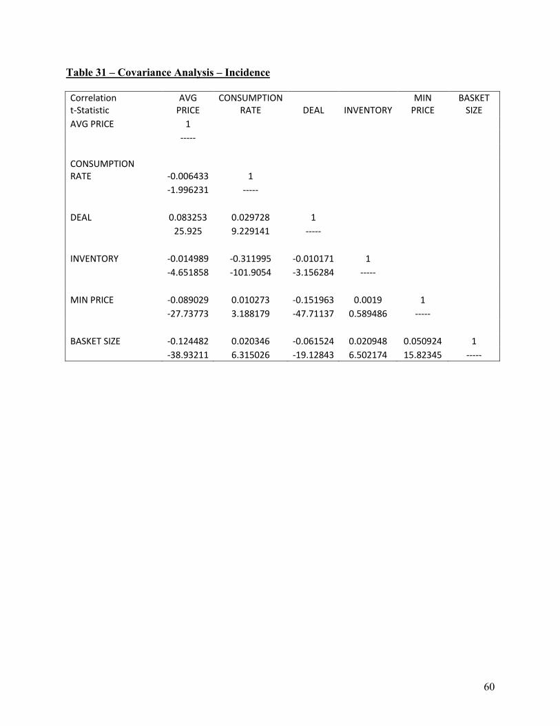
Table 31 – Covariance Analysis – Incidence
Correlation t-Statistic
AVG PRICE
CONSUMPTION RATE DEAL INVENTORY
MIN PRICE
BASKET SIZE
AVG PRICE 1 ----- CONSUMPTION RATE -0.006433 1 -1.996231 ----- DEAL 0.083253 0.029728 1 25.925 9.229141 -----
INVENTORY -0.014989 -0.311995 -0.010171 1 -4.651858 -101.9054 -3.156284 ----- MIN PRICE -0.089029 0.010273 -0.151963 0.0019 1 -27.73773 3.188179 -47.71137 0.589486 ----- BASKET SIZE -0.124482 0.020346 -0.061524 0.020948 0.050924 1 -38.93211 6.315026 -19.12843 6.502174 15.82345 -----
61
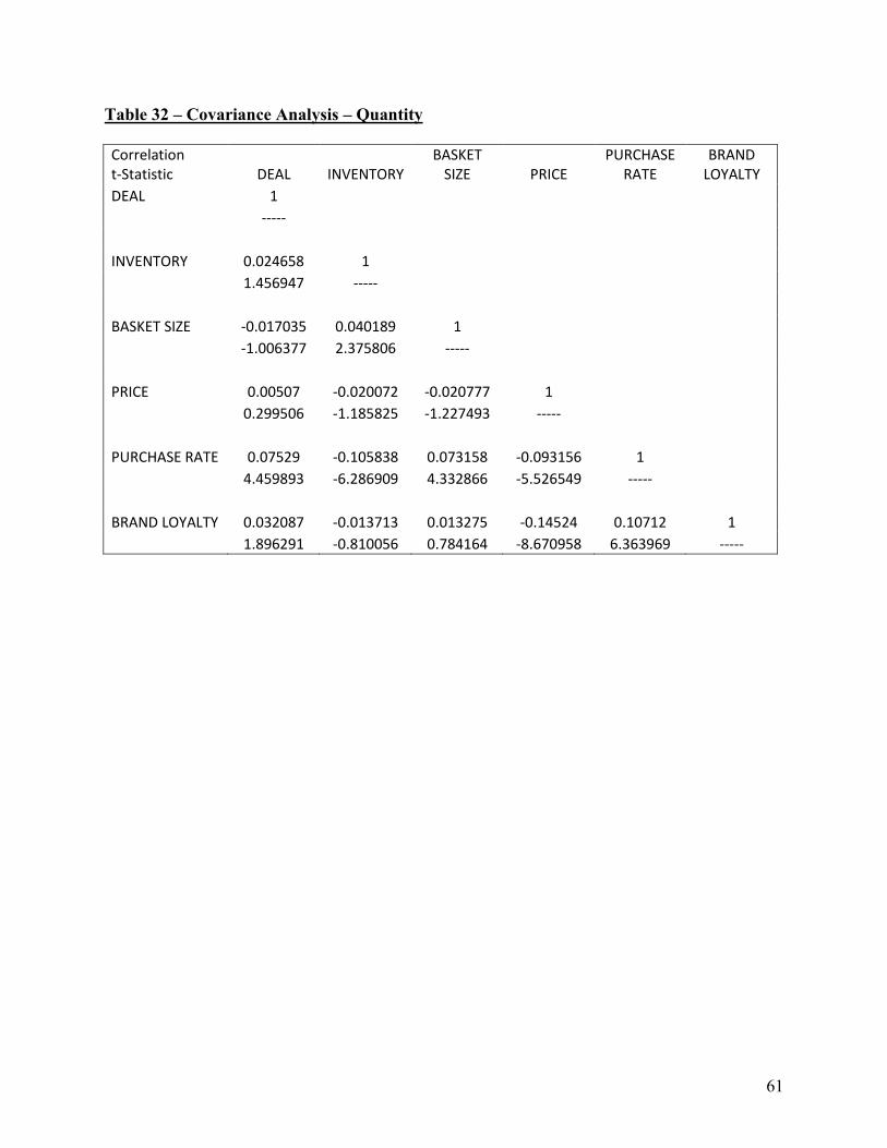
Table 32 – Covariance Analysis – Quantity
Correlation t-Statistic DEAL INVENTORY
BASKET SIZE PRICE
PURCHASE RATE
BRAND LOYALTY
DEAL 1 ----- INVENTORY 0.024658 1 1.456947 ----- BASKET SIZE -0.017035 0.040189 1 -1.006377 2.375806 -----
PRICE 0.00507 -0.020072 -0.020777 1 0.299506 -1.185825 -1.227493 ----- PURCHASE RATE 0.07529 -0.105838 0.073158 -0.093156 1 4.459893 -6.286909 4.332866 -5.526549 ----- BRAND LOYALTY 0.032087 -0.013713 0.013275 -0.14524 0.10712 1 1.896291 -0.810056 0.784164 -8.670958 6.363969 -----