The Impact of Capital and Liquidity Regulation: Evidence from European Banks Armen Arakelyan a CUNEF Artashes Karapetyan b Norges Bank This version: October 2014 Abstract Under the assumption of efficient and perfect capital markets, lower leverage leads to lower equity risk and hence lower required return on it, leaving weighted average cost of capital un- changed. We test this using data from listed European banks. We find that lower leverage (as well as higher liquidity) decrease equity risk. However, low risk banks offer higher or the same risk-adjusted stock returns in excess of risk-free rate. Under the assumption of riskless debt, calibration results show that a 10 percentage point increase in capital requirements brings about a 45 basis point increase in the weighted average cost of capital. JEL classification: G01, G12, G21, G28 Keywords: Bank regulation, cost of capital, liquidity, low risk anomaly a A. Arakelyan is from Department of Finance, University College of Financial Studies (CUNEF), c/Leonardo Prieto Casto, 2, 28040 Madrid, Spain. Tel: +34 91 448 08 92, email: [email protected]. b A. Karapetyan is from Norges Bank Research, Bankplassen 2, P.O. Box 1179 Sentrum, Norway. Tel: + 47 22 31 62 52, e-mail: Artashes.Karapetyan@norges- bank.no. We thank G. Rubio, E. Duca, L. Swinkels, seminar participants at CUNEF, Norges Bank, EFMA 2014, and the 2014 Conference on Econometric Methods for Banking and Finance (Banco de Portugal) for valuable comments and suggestions. The views expressed in the paper do not represent those of Norges Bank. All remaining errors are ours.
Transcript
The Impact of Capital and Liquidity Regulation: Evidence
from European Banks
Armen Arakelyana
CUNEF
Artashes Karapetyanb
Norges Bank
This version: October 2014
Abstract
Under the assumption of efficient and perfect capital markets, lower leverage leads to lower
equity risk and hence lower required return on it, leaving weighted average cost of capital un-
changed. We test this using data from listed European banks. We find that lower leverage (as
well as higher liquidity) decrease equity risk. However, low risk banks offer higher or the same
risk-adjusted stock returns in excess of risk-free rate. Under the assumption of riskless debt,
calibration results show that a 10 percentage point increase in capital requirements brings about
a 45 basis point increase in the weighted average cost of capital.
JEL classification: G01, G12, G21, G28
Keywords: Bank regulation, cost of capital, liquidity, low risk anomaly
aA. Arakelyan is from Department of Finance, University College of Financial Studies (CUNEF), c/Leonardo PrietoCasto, 2, 28040 Madrid, Spain. Tel: +34 91 448 08 92, email: [email protected]. bA. Karapetyan is from Norges BankResearch, Bankplassen 2, P.O. Box 1179 Sentrum, Norway. Tel: + 47 22 31 62 52, e-mail: [email protected]. We thank G. Rubio, E. Duca, L. Swinkels, seminar participants at CUNEF, Norges Bank, EFMA 2014, andthe 2014 Conference on Econometric Methods for Banking and Finance (Banco de Portugal) for valuable commentsand suggestions. The views expressed in the paper do not represent those of Norges Bank. All remaining errors are ours.
1 Introduction
Highly leveraged financial institutions create negative externalities: a small decrease in the
asset value of a highly leveraged bank can lead to distress and potential insolvency. In an
interconnected financial system, this can cause the system to freeze, and may lead to severe
repercussions for the rest of the economy. Governments often spend large amounts on bailouts
and recovery efforts to minimize social damage. Whereas avoiding such systemic risk and its social
costs is a major objective of financial regulation, market participants act in their own interests
and pay little attention to systemic concerns: the role of financial regulation is to safeguard the
well functioning of the financial industry.
After the experience of the recent financial crisis policy makers and academics have been
actively debating whether banks should reduce their leverage. The purpose of using relatively
more equity funding is to avoid that variations in asset values lead to distress and insolvency.
Most bankers, however, consider equity as a costly source of bank finance: since equity is more
costly than debt, then more of it will increase the weighted average cost of capital.
A number of recent studies, on the other hand, have argued that the overall cost of capital will
remain unchanged despite changes in capital structure. Admati et al. (2011) consider arguments
of expensive equity as fallacy and bring up the classical example of Modigliani-Miller: since the
increase in capital provides further protection to shareholders reducing their risk, they will require
lower rates of return in the more capitalized bank.
Thus whether or not higher capital requirements affect banks’ overall cost of capital (and
therefore lending rates and economic activity) is an empirical concern. In this paper we address
this concern by using comprehensive data from listed European Banks. Our main objective is to
evaluate the capital requirements and the risk-return relationship in the banking stock market.
Similar to Baker and Wurgler (2014), our methodology proceeds in two steps. First, we esti-
mate, the impact of leverage on bank equity risk and, second, the relation between equity risk and
2
cost of bank equity or the overall cost of capital. In addition we estimate the impact of liquidity
regulation on bank equity risk. Empirical evidence on the risk return relationship is mixed. Our
motivation stems particularly from the potential interaction between capital requirements and
the low risk anomaly within the stock market. That is, while stocks have on average earned
higher returns than less risky asset classes (such as corporate bonds, which in turn have earned
higher returns than government bonds or other riskless assets) the risk-return relationship within
the stock market has historically been flat or even inverted.
Fama and French (1992), Baker et al. (2011) find a flat or negative relationship between
a stock’s systematic risk, as measured by its stock market beta, and its subsequent returns.
Similar patterns of negative relationship have also been documented between idiosyncratic risk
and returns in the U.S. as well as many international stock markets (see, for instance, Ang et al.
(2009)). These studies suggest that there is a low risk anomaly on average within the stock
market. Therefore, a relevant question for bank capital regulation is whether this holds within
banks specifically. Indeed, the low risk anomaly might not be present in banks at all. All of
these studies suggest that risk is not necessarily rewarded, and the relevant question is whether
or not this is the case for the banking stocks in Europe. Does the cost of equity fall with capital
requirements as the Modigliani-Miller logic predicts? Or does it not fall by enough, or actually
increase, as bankers and the low risk anomaly would imply? Baker and Wurgler (2014) bring
evidence supporting low risk anomaly from the U.S.. We conclude the same from banks across
major Western European economies in the period from 1990 to 2014, and to the best of our
knowledge this is the first attempt to do so.
The choice of capital is endogenous to the riskiness of banks’ assets: highly leveraged financial
institutions would not opt for very risky investments fearing bankruptcy, while those with high
capital would have more appetite for risk. To address this, we follow Baker and Wurgler (2014)
and proceed in two steps in the regression analysis: the first step is to relate bank equity risk
3
estimated from markets to capital ratios from annual accounting data. In the second step, we
regress realized returns on equity to bank equity betas. Our most important finding is that while
the expected relationship in the first step is confirmed, we see no positive, or even negative,
relationship between risk and excess return in the second one.
The two steps together also allow us to calibrate the effect of increased capital requirements
on the cost of equity as well as on weighted average cost of capital, under some assumptions
made about the riskiness of debt. As a benchmark case, under the assumption of riskless debt,
we find that a 10 percentage point increase in capital requirement bring about a 45 percentage
point increases in WACC. Finally, in some of the analysis we also look at idiosyncratic risk in
addition to beta. The key insight from the procedure is that the established link in the first step
is an attenuated one: absent endogeneity, increases in capital ratios would have translated to
more pronounced decreases in equity betas. In the second step, this would have resulted in at
least as much an increase in excess return, yielding WACC even higher.
Since we are studying international stocks, we make certain assumption about the extent
of integration of asset markets across countries. There may be problems if there is absence of
integrated asset pricing in the region we cover. Even in the case when we have the correct asset
pricing model, let’s assume for instance CAPM, (and suppose we have integrates asset pricing),
betas with respect to the whole region’s market portfolio explain expected returns on all assets,
but then local version of CAPM should not work. For example, betas with respect to the U.K.
market portfolio should not explain expected returns on all U.K. assets. On the other hand if
pricing is not regionally integrated, the international CAPM should fail if a local CAPM prices
assets in each market. Following Fama and French (2012), we will assume that the European
region is integrated enough and can be treated as one market.
Banking literature typically studies loan portfolios of banks, where the prices of loans are hard
to measure on a market basis on a high enough frequency.In this regard, our paper is different
4
from the typical banking literature, and in terms of methodology closer to asset pricing literature
of mainly non-financial firms, as well as the few recent studies on banking equity. From the latter
group, perhaps closest to our paper is Baker and Wurgler (2014) and Kashyap et al. (2010), who
did similar analysis for the U.S..1
2 Betas, capital, and return
Standard theory of the firm predicts that lower leverage reduces risk and therefore cost of
equity, under the assumptions of perfect and efficient capital markets.2 In this paper, we confirm
the first part of the theory, namely that the risk of bank goes down as leverage decreases. Our
measures of capitalization show that the most capitalized banks have the lowest equity betas.3
Interestingly, these differences are affected (i.e., attenuated) by two factors. First, they would be
more pronounced if banks with riskier assets did not choose to have larger capital; because riskier
assets increase bankruptcy probability, banks will want to increase their capital cushion. Thus,
such a move is endogenous, and reduces the slope between capital ratios and beta.
Second, from some point on part of the asset risk is eventually borne by debtholders. This
is true for highly leveraged banks; if a highly leveraged bank further increases its leverage, it is
likely to increase its bankruptcy probability and therefore the risk for debtholders. But because
debt risk rises, beta of debt will rise too, thus giving room for a more attenuated rise in equity’s
beta, thereby flattering the relationship between beta and capital ratios.
According to the second part of the theoretical argument, a reduction of equity beta should
be reflected in a reduction of the cost of equity. We however show that this is not the case.
The reduction of beta is generally invariant to returns, in line with empirical evidence on the
1 King (2009) estimates cost of equity in a single factor CAPM model, while Maccario et al. (2002) estimate banks’cost of equity using analyst earnings’ forecast.
2Modilgiani-Miller irrelevance predicts that the overall cost of capital is unchanged3In fact, this is also true for idiosyncratic risk measures.
5
low risk anomaly. While in efficient capital markets banks with higher capital ratios should have
lower equity returns, capital structure is endogenous due to risk aversion and bankruptcy costs,
rendering the cross-sectional analysis of capital ratios and beta erroneous.
To understand the causal effect of an increase in (exogenous) capital requirements we take into
account the endogenous choice of (risky) banks for (high) capital, similar to Baker and Wurgler
(2014). These effects will tend to reduce the effect of higher capital (as caused by regulation) on
equity beta. But if one ignores the latter and still finds the expected relationship between capital
and empirical equity betas, then it means that the exogenous effects will be at least as large.
The main arguments in the discussion of whether increased equity ratios will make the cost
of capital higher, may be summarised by looking at the equation relating cost of assets to the
cost of equity, the cost of debt and the equity ratio
βAsset =E
D + EβEquity +
D
D + EβDebt.
In this equation the cost of equity is typically higher than the cost of debt. What is often
referred to as the Miller and Modigliani (MM) argument, is that the left hand side of this equation
does not change if the equity ratio changes. If the equity share is increased, the volatility of
equity is reduced and so is the cost of equity. The cost of debt, on the other hand, will either
remain unchanged or decrease. Even though the individual elements of the right hand side of the
equations will (or may, in case of debt) change, the sum of the elements will not change. What
seems to be banks’ argument is that the left hand side of the equation does change when the
equity share is increased. In other words, the cost of capital is not fixed. Increasing the equity
ratio will make the cost of capital higher because ”cheap” debt is replaced by ”expensive” equity.
Even though the cost of equity is reduced, this reduction will not be large enough to avoid that
an increase in the cost of capital. Bankers use this line of reasoning when arguing against stricter
capital regulation and against stricter capital regulation in one country than another. Note that
6
the above yields
βEquity =D + E
EβAsset −
D
EβDebt (1)
In the two step analysis of the impact of heightened capital regulation on cost of capital, the
estimation of the above relationship will be the first step. The relationship between leverage
and equity beta is linear whenever debt is riskless, and the slope is equal to the asset beta. As
mentioned before, whenever leverage is very high and debt is no longer riskless, further increase
in leverage will be accompanied by increases in debt beta, and therefore equity beta will not
increase at the same pace: the increase in asset risk is now partially borne by debtholders. Such
effect is in addition, and amplifies the attenuating effect of endogenous capital selection.
2.1 Liquidity requirements in Basel III Regulation
In December 2009 the Basel committee introduced new rules to the existing Basel II regulation,
known as Basel III. In addition to revised capital adequacy requirements, Basel III proposed two
new liquidity requirements: the liquidity coverage ratio (LCR) and the net stable funding ratio
(NSFR). Essentially, banks are required to hold sufficient amount of high quality liquid assets
(HQLA) to meet their net cash requirements until day 30 of the stress scenario (see BCBS (2014)
for details of NSFR and BCBS (2013) for detailed definition of HQLA and LCR).4 Holding liquid
instruments such as cash or government bonds can reduce asset beta, the overall risk of the bank,
and equity beta. With the low risk anomaly, this may then increase the cost of bank equity.
The calculation of the cost to meet the NSFR is not trivial and will depend on definition of the
4The aim of LCR is ensure that banks can withstand a 30-day liquidity stress scenario. The NSFR is a longer-termliquidity ratio designed to address maturity mismatches between banks’ assets and liabilities over one-year horizon. Itprovides incentives for banks to use stable sources of funding, such as stable deposits, equity and long-term liabilities.The banks are set to report new ratios from 2015. The implementation of the new Basel III regulations will be carriedout gradually until 2019. Particularly, by the beginning of 2019 the banks should have reached 100% level for LCR. SeeAppenidx A for the timing and implementation of Basel III requirements.
7
ratio. It requires assumptions about the composition of banks assets and liabilities, and estimates
of the returns on different assets and the costs of different liabilities. This detailed information
is not disclosed in a banks financial statements, but is being collected by the Basel Committee
on banking Supervision (BCBS) through the Quantitative Impact Study (QIS). Below we follow
King (2009), where the estimates are based on the December 2009 proposal of the NSFR, which
was modified in July 2010 with the implementation date moved out to 2018.
3 Data and Summary Statistics
We use all European companies classified as banks by Industry classification Benchmark (ICB)
from Bloomberg. More specifically, our broad sample includes both active and non-active banks
domiciled in 43 European countries.5 The data are from January 1990 to September 2014. We
mostly carry out our analysis for banks from Eurozone that joined the monetary union before
2001, the U.K., Switzerland and Scandinavia, except Iceland. We use the full sample with Central
European countries in robustness checks.
Our market data for banks include end-of-month observations for closing share prices, market
capitalization, and monthly total holding period returns.6 Share prices and holding period returns
are for one outstanding share class of a bank, as identified by the Primary Security Ticker in
Bloomberg. Our accounting data for banks include major items from Balance Sheet, Income, and
Cash Flow statements, and information on notes to those financial statements. The accounting
data are available on a quarterly basis from 1997 Q1.7 All variables from market and accounting
5Active banks are publicly traded banks as of now, and non-active banks are those that were once active.6Holding period returns include gross dividends, and represent month-end-day to month-end-day total return values.
See Appendix B for detailed variable definitions.7In the earlier version of this paper entitled “Impact of Higher Capital Requirements on Cost of Capital: Evidence
from European Banks”, we take our banking and accounting data from Worldscope/Datastream, where accountingvariables were only annual. Results are similar to the ones reported in this paper for the effects of capital requirementsand are available upon request.
8
samples are denominated in USD. The reason for using a single currency is to ease the comparison
among banks from various countries with i) different currencies and ii) currencies that have
changed over our sample period.
Returns on portfolios of Fama-French 3 factors for Europe are taken from Kenneth French’s
data library. All factor returns are in US dollars. Risk free rates are the yields from one-month
US Treasury bills, taken from Kenneth French. Additionally, we also obtain the total return
series for EURO STOXX 50 and STOXX Europe 600 indexes and time series of EURIBOR for
one and three month maturities. Whenever available, we use gross total returns for the indexes.
We proceed by merging accounting data with market returns. Similar to Fama and French
(1992), we ensure that the accounting variables are known prior to the returns that they are
used to explain. To this end, we match the accounting data for all fiscal quarter-ends in month t
with the market returns for months t+ 1 to t+ 3. We allow one month gap between quarter-end
month and the returns because quarterly fillings made by public companies follow the end of each
quarter (with delay). Most companies file in January, April, July and October.
For capital adequacy analysis we consider the following measures: i) Total common equity to
Total assets, ii) Tangible Equity to Total Assets iii) Total Risk-Based Capital to Total Assets,
iv) Tier 1 capital to Risk Weighted Assets (RWA), and v) Total Risk-Based Capital to RWA.8
As for the liquidity requirements, we consider i) Cash and near cash items divided by Short-
Term Debt as a proxy for LCR and ii) a proxy for NSFR, following King (2010). We recall that
LCR and NSFR are not directly observable as the constituents used to calculate these measures
are not available on financial statements.
8Regulatory capital consists of other elements than equity. Basel III uses the categories Tier 1 and Tier 2 capital forregulatory capital. Tier 1 consists of Common Equity Tier 1 and Additional Tier 1 (AT1) capital. AT1 capital is hybridcapital with “equity-like” characteristics. The minimum regulatory capital requirements are expressed as a minimumlevel of the ratio of regulatory capital to risk weighted assets. Banks may therefore improve their regulatory capitalratios by increasing the regulatory capital or by reducing risk weighted assets. There is therefore not a one-to-onerelationship between higher regulatory capital requirements and higher equity ratios. Basel III, however, does implythat most banks have to increase their equity levels. In addition, Basel III introduces a minimum requirement for theequity ratio.
9
3.1 Summary Statistics
Table 1 shows the number of banks in each period and each country. Our primary sample
includes bank-months for which we can calculate a valid beta, with at least 24 monthly holding
period return observations, a valid market capitalization, and at least one holding period return
following a valid beta.
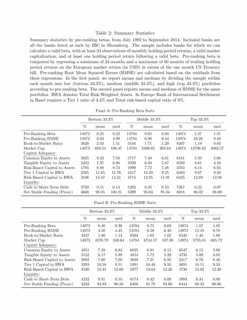
Table 2 provides summary statistics by pre-ranking betas, from July 1990 to October 2013.
Pre-ranking beta is computed by regressing a minimum of 24 months and a maximum of 60 months
of trailing holding period returns on the European market return, in excess of the one month
US Treasury bill. The market return for the European region is taken from Kenneth French’s
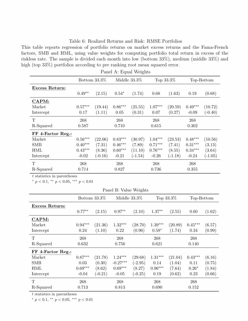
data library. In some of the analysis we also look at idiosyncratic risk in addition to beta. We
take the root mean square error (RMSE) from pre-ranking beta regressions as our measure of
idiosyncratic risk. In the first panel, we report means and medians by dividing the sample within
each month into low (bottom 33.3%), medium (middle 33.3%), and high (top 33.3%) portfolios
according to pre-ranking beta. The second panel reports means and medians of RMSE for the
same portfolios. The pre-ranking betas are 0.28 and 1.29 in the bottom and top pre-ranking beta
percentiles, respectively. Unlike non-financial firms, there is a positive relationship between bank
size and risk; market capitalization increases with beta. Big banks might have other units, such
as investment banking, brokerage, and asset management. The investment carried out by these
units tend to produce returns that co-move with the overall stock market returns.
Figure 1 plots the time series of average betas (both equal and value weighted) for each
pre-ranking beta percentile. There is an upward trend in the time series of pre-ranking betas.
Pre-ranking betas also seem to increase during financial crisis. In particular, there is a noticeable
increase in betas after mid 1997 and 2007, respectively. The former is due to the Asian financial
crisis of 2007, and subsequent Russian crisis of 1998, while the latter is associated with the
subprime crisis that originated in the U.S. in mid 2007.
10
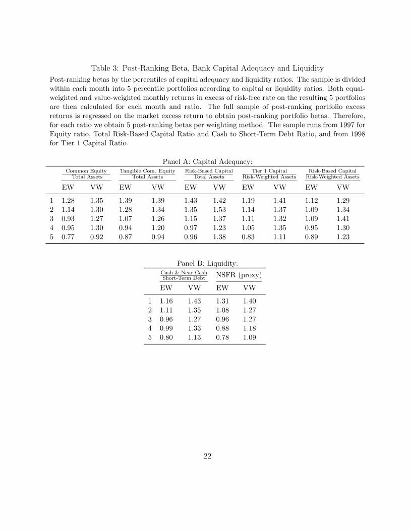
Table 3 provides the summary statistics of post-ranking portfolio betas by capital and liquidity
ratio percentiles. The sample is divided within each month into five percentile portfolios according
to capital or liquidity. We follow Fama and French (1992) to calculate post-ranking betas. In
particular, we first calculate monthly returns in excess of risk-free rate on different portfolios for
each month and capital/liquidity ratio. Portfolio returns in each percentile of each capital or
liquidity ratio are either equal or value weighted. Second, we regress the full sample of post-
ranking portfolio excess returns on the market excess return to obtain post-ranking portfolio
betas.
In all specifications for capital adequacy ratios higher capital is associated with lower post-
ranking portfolio betas. As already highlighted in Section 2, the difference between portfolio
betas of top and bottom percentiles of capital adequacy ratios is likely to be attenuated because
of the endogenous choice of bank capital. This difference is also smaller for value weighted post-
ranking betas as compared to the difference for equal-weighted post-ranking betas. Banks with
higher capital adequacy ratio (e.g. in the 5th percentile) can still have high betas as riskier banks
a priori might prefer to hold higher capital to avoid bankruptcy or high bankruptcy costs in the
future. On the other hand, higher beta banks tend to have higher market capitalization. Due to
those two observations, the value weights, which are based on the market capitalization, “inflate”
the realized betas in the higher capital ratio percentiles (e.g. in the 5th percentile). Therefore,
the observed difference in top and bottom value-weighted betas is smaller.
Higher liquidity is also associated with lower post-ranking betas. Similar to the capital ade-
quacy ratios, the observed difference between top and bottom realized betas within liquidity ratio
percentiles is smaller for value-weighted specification.
11
4 Empirical Analysis
4.1 Equity beta and capital ratio
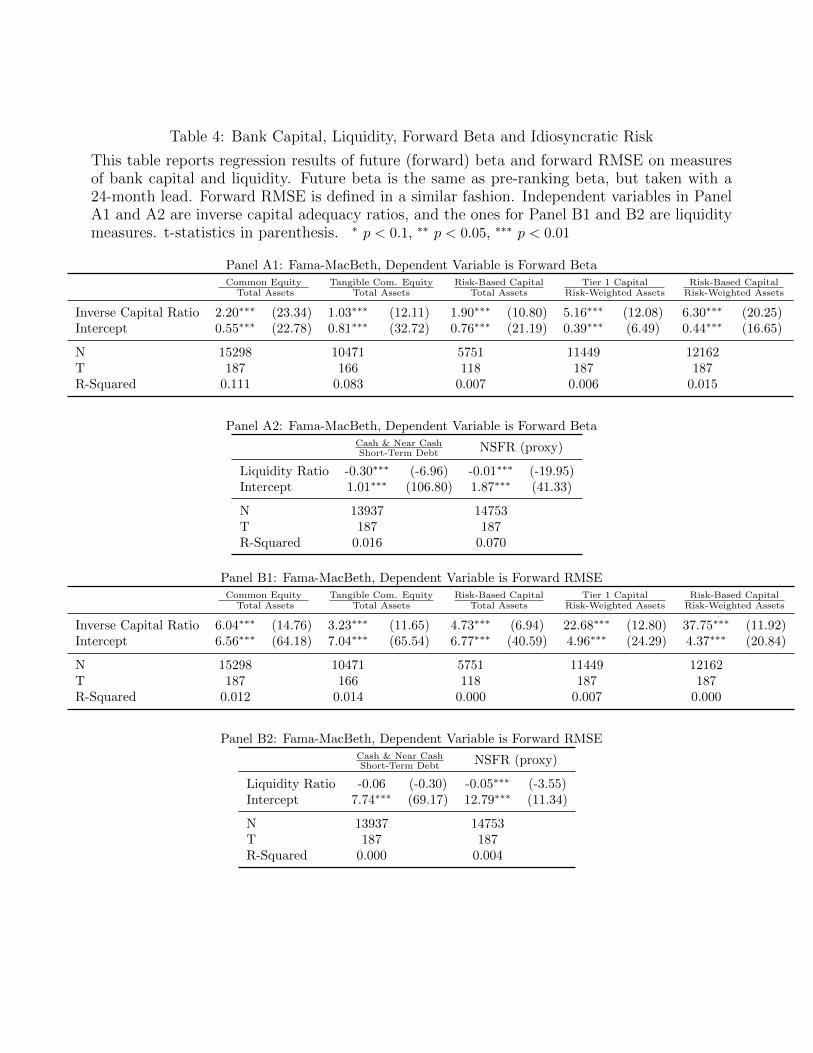
Table 4 shows Fama-MacBeth regression results of forward beta and idiosyncratic risk on
inverse equity capital, the specification suggested by equation (1), for all banks. Additionally,
we run Fama-MacBeth regressions of forward beta and idiosyncratic risk on liquidity measures.
Forward beta is the pre-ranking beta taken with a 24 month lead. Forward RMSE is defined in
a similar fashion. In panels A1 and A2 the dependent variable is the forward beta, and in Panels
B1 and B2 the dependent variable is the forward RMSE. We use the Fama and MacBeth (1973)
procedure, which gives equal weight to each cross section in the estimation.
If capital choice were exogenous and debt were riskless, we would expect the intercepts in the
regressions of forward betas on inverse capital ratios to be zero, and the slopes to be equal to
the average bank asset betas. Consistent with the endogenous choice of capital, we observe that
the intercepts are greater than zero and statistically significant in all specifications for capital
adequacy. The slope coefficients are lower that what we would have obtained if the leverage choice
were not endogenous. We find similar qualitative results for the idiosyncratic risk, measured by
RMSE. Overall, the results of Table 4 confirm the hypothesis that higher leverage increases equity
risk.
Panel A2 of Table 4 reveals that the regression slopes in the regression of forward betas
on liquidity measures are negative and statistically significant. We tentatively conclude that
heightened liquidity requirements decrease equity risk for banks.
4.2 Returns and cost of equity
Should lower betas reduce bank cost of equity as the argument of MM indicates? To address
this question, we assign banks to three portfolio groups according to pre-ranking beta. Afterwards,
12
we run a series of OLS regressions, controlling for common risk factors, such as the overall market
factor (CAPM), and factors related to firm size, and book-to-market equity (Fama-French 3-factor
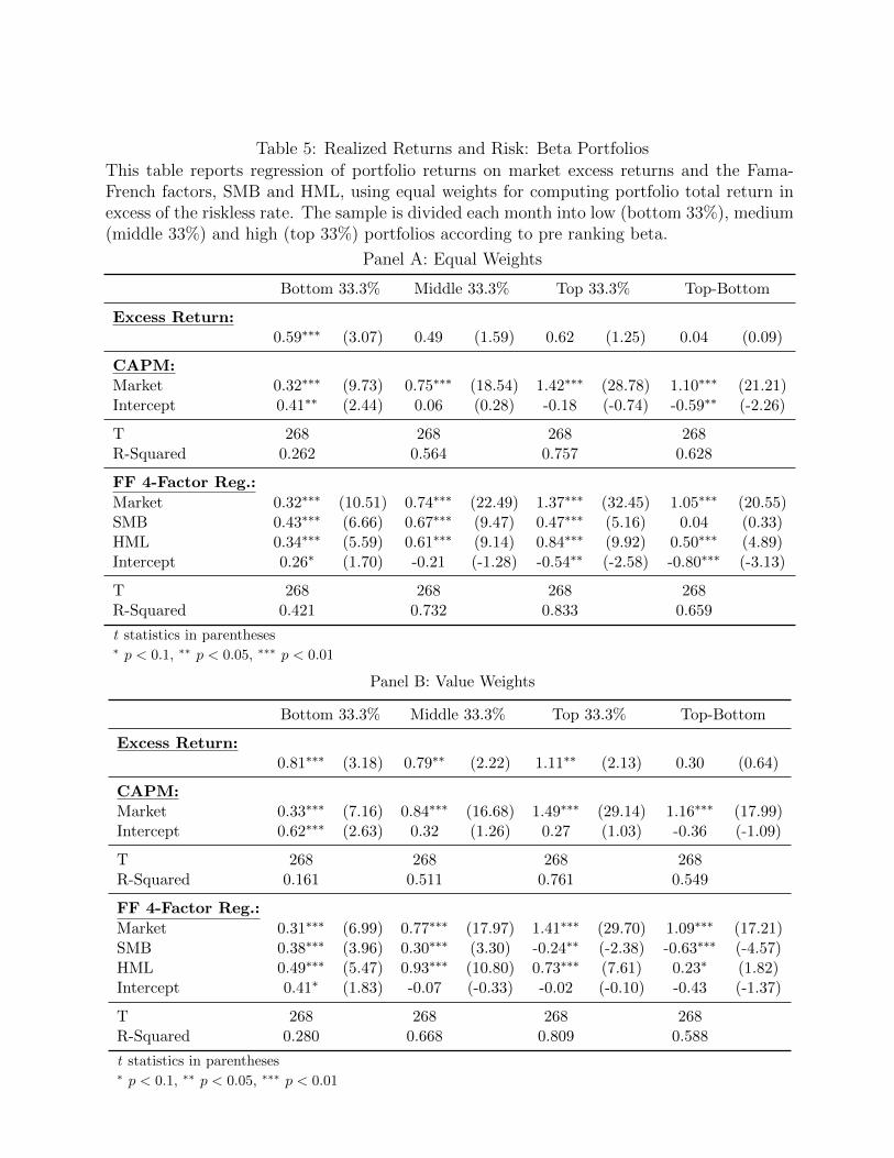
model). Table 5 provides the results of the OLS regressions. Under the CAPM model, the realized
betas (equal weighted) increase from 0.32 to 1.10 for bottom and top beta portfolios, respectively.
However, the risk-adjusted monthly returns in excess of the riskless rate (alphas) decline from
low beta to high beta portfolios. The difference between top and bottom portfolio alphas is -59
basis points, and this difference is statistically significant. The alphas also decline relative to
Fama-French 3-factor model. These results indicate that the security market line is flat relative
to the CAPM model. Low beta banks particularly seem to be underpriced; the point estimates
of alphas of the lowest beta portfolios are positive and significant in all specifications. Similar
pattern can be discerned for value-weighted portfolios, albeit the statistical significance is weak.9
Therefore, theory does not match the data on stock returns for banks. We indeed document
that less leverage does reduce equity risk and equity beta, but we are unable to see that lower
beta translates into lower risk adjusted returns. The evidence above suggests that lower risk
banks have the same or higher risk adjusted excess returns than higher risk banks.
4.3 Calibration
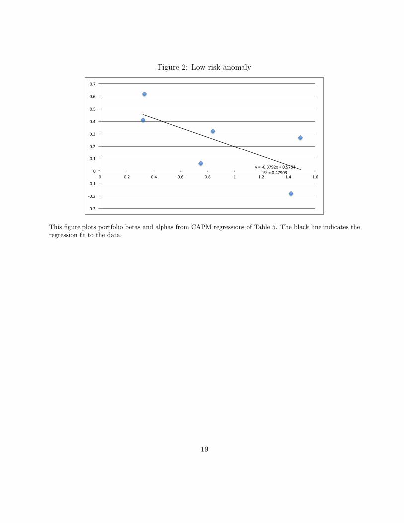
Following Baker and Wurgler (2014) we suppose that the CAPM holds but with a low risk
anomaly (i.e. higher beta equities underperform their CAPM benchmark and lower beta equites
outperform them), and returns can be explained by ri = (βi − 1)γ + rf + βirp, where γ = ∂α∂β
measures the extent of the low risk anomaly. Indeed, as our Table 5 and 6 show, higher betas are
related with lower alphas. This can be better seen in Figure 2 where we plot the equal weighted
and value weighted alpha-beta relationships for CAPM regressions (see Table 5).
With the above returns equation in mind and assuming that debt is correctly priced by
9Appendix C provides the regression results of the CAPM and Fama-French 3-factor model for 5 and 10 beta-sortedportfolios. The results are qualitatively similar to the ones of 3 beta-sorted portfolios.
13
CAPM, WACC can be expressed by WACC = e(βe− 1)γ+ rf +βarp. To see the effect of higher
capital requirements, we need to difference the above equation, which will yield ∆WACC =
means that the change in average cost of capital is equal to γ(e− e∗), an assumption which is not
far from being innocuous as the effects of changing debt beta are rather small. Indeed, means of
capital ratios are between 5.6 and 13 percent for tangible equity ratio and risk-based capital to
risk-weighted assets ratio, respectively, and average bank beta is 0.73 in our sample. This means
that βa are quite small. Using Table 5 we can get an estimate of the low risk anomaly: the linear
regression of alpha and beta provides an estimate of γ = 0.38. With riskless debt, a 10 percentage
point increase in capital requirements will bring about around 45 basis points (= 38 × 12 × 0.1)
increase in cost of capital.
5 Discussion and concluding remarks
There are a number of reasons for regulatory increase in minimum capital requirements:
agency problems in banks, asymmetric information, international coordination, bank governance,
tax benefits of debt, government subsidies, shadow banking, and so on. Despite the costly fric-
tions, there is a pervasive view underlying most discussions of capital regulation that equity is
expensive, and that equity requirements, while having substantial benefits in mitigating problems
causing instability, impose costs on the financial system and possibly on the economy. Bankers,
policy makers and regulators are particularly concerned by assertions that increased equity re-
quirements would restrict bank lending and would impede economic growth. Possibly as a result
of such pressure, the proposed Basel III requirements, while moving in the direction of increasing
capital, still allow banks to remain very highly leveraged.
However, the view on the impact of capital requirements on cost of capital is two-faceted.
14
Many economists still maintain that weighted average cost of capital will remain unchanged.
Following Modigliani and Miller, Admati et al. (2011) claim that because the increase in capital
provides downside protection that reduces shareholders’ risk, shareholders will require a lower
expected return to invest in a better capitalized bank.
We find that this theory does not match the data on stock returns for banks. While the
evidence does show that less leverage reduces equity risk, there is still a role for the low risk
anomaly in European bank equities: we document that lower risk banks have the same or higher
risk adjusted excess returns than higher risk banks. The evidence contained in European market
data suggests that increasing capital requirements by around 10 percent may be associated with
45 basis point increase in average cost of capital.
15
References
Admati, A., P. DeMarzo, M. Hellwig, and P. Pfeiderer (2011). Fallacies, Irrelevant Facts, and
Myths in the Discussion of Capital Regulation: Why Bank Equity is Not Expensive. Stanford
University, Working Paper.
Ang, A., R. J. Hodrick, Y. Xing, and X. Zhang (2009). High Idiosyncratic Volatility and Low
Returns: International and Further U.S. Evidence. Journal of Financial Economics 91 (1),
1–23.
Baker, M., J. Bradley, and J. Wurgler (2011). Benchmarks as Limits to Arbitrage: Understanding
the Low-Volatility Anomaly. Financial Analysts Journal 67 (1), 1–15.
Baker, M. and J. Wurgler (2014). Do Strict Capital Requirements raise the Cost of Capital:
Banking Regulation and The Low Risk Anomaly. Harvard University, Working Paper.
BCBS (2013). Basel III: The Liquidity Coverage Ratio and liquidity risk monitoring tools. BIS.
BCBS (2014). Basel III: The Net Stable Funding Ratio. Consultative Document (January).
Fama, E. and K. French (1992). The Cross Section of Expected Stock Returns. Journal of
Finance 47 (2), 427–465.
Fama, E. and K. French (2012). Size, Value, and Momentum in International Stock Returns.
Journal of Financial Economics 105 (3), 457–472.
Fama, E. and J. D. MacBeth (1973). Risk, Return, and Equilibrium: Empirical Tests. Journal
of Political Economy 81 (3), 607–636.
Kashyap, A. K., J. C. Stein, and S. G. Hanson (2010). An Analysis of the Impact of of ‘Substen-
tially Heightened’ Capital Requirements on Large Financial Institutions. Harvard University,
Working Paper.
16
King, M. (2009). The cost of equity for global banks: a CAPM perspective from 1990 to 2009.
BIS Quarterly Review.
King, M. (2010). Mapping capital and liquidity requirements to bank lending spreads. Bank for
International Settlements, Working Paper No. 324.
Maccario, A., A. Sironi, and C. Zazzara (2002). Is banks’ cost of equity capital different across
countries? Evidence from the G10 countries major banks. Libera Universita Internazionale
degli Studi Sociali (LUISS) Guido Carli, working paper.
17
Figure 1: Pre-Ranking Betas
0.5
11.
52
Pre
Ran
king
Bet
a (E
W)
01/19
90
01/19
95
01/20
00
01/20
05
01/20
10
01/20
15Aug
'07Aug
'07Sep
'08
date
Top 33.3%Middle 33.3%Bottom 33.3%
0.5
11.
52
Pre
Ran
king
Bet
a (V
W)
01/19
90
01/19
95
01/20
00
01/20
05
01/20
10
01/20
15Aug
'07Aug
'07Sep
'08
date
Top 33.3%Middle 33.3%Bottom 33.3%
The top and bottom panels plot the time series of equal- and value-weighted pre-ranking betas, respectively.Observation are from July 1992 to September 2014. The sample is divided into three equal parts based onpre-ranking beta sorts, top, middle, and bottom, market weighted. Included banks are all the banks classifiedas such by ICB in Bloomberg. The sample includes banks for which we can calculate a valid beta, with atleast 24 observations of monthly holding period return, a valid market capitalization, and at least one holdingperiod return following a valid beta. Pre-ranking beta is computed by regressing a minimum of 24 monthsand a maximum of 60 months of trailing holding period returns on the European market return in excess ofthe one month US Treasury bill. 18
Figure 2: Low risk anomaly
y = -‐0.3792x + 0.5754 R² = 0.47903
-‐0.3
-‐0.2
-‐0.1
0
0.1
0.2
0.3
0.4
0.5
0.6
0.7
0 0.2 0.4 0.6 0.8 1 1.2 1.4 1.6
This figure plots portfolio betas and alphas from CAPM regressions of Table 5. The black line indicates theregression fit to the data.
Number of banks in each country by five-year time periods and overall, from July 1992 to September 2014.Included banks are all the banks classified as such by ICB from Bloomberg. The sample includes banks forwhich we can calculate a valid beta, with at least 24 observations of monthly holding period returns, a validmarket capitalization, and at least one holding period return following a valid beta.
20
Table 2: Summary Statistics
Summary statistics by pre-ranking betas, from July 1992 to September 2014. Included banks areall the banks listed as such by IBC in Bloomberg. The sample includes banks for which we cancalculate a valid beta, with at least 24 observations of monthly holding period returns, a valid marketcapitalization, and at least one holding period return following a valid beta. Pre-ranking beta iscomputed by regressing a minimum of 24 months and a maximum of 60 months of trailing holdingperiod returns on the European market return (in USD) in excess of the one month US Treasurybill. Pre-ranking Root Mean Squared Errors (RMSE) are calculated based on the residuals fromthese regressions. In the first panel, we report means and medians by dividing the sample withineach month into low (bottom 33.3%), medium (middle 33.3%), and high (top 33.3%) portfoliosaccording to pre-ranking beta. The second panel reports means and medians of RMSE for the sameportfolios. RWA denotes Total Risk-Weighted Assets. In Europe Bank of International Settlementin Basel requires a Tier 1 ratio of 4.4% and Total risk-based capital ratio of 8%.
Table 3: Post-Ranking Beta, Bank Capital Adequacy and Liquidity
Post-ranking betas by the percentiles of capital adequacy and liquidity ratios. The sample is dividedwithin each month into 5 percentile portfolios according to capital or liquidity ratios. Both equal-weighted and value-weighted monthly returns in excess of risk-free rate on the resulting 5 portfoliosare then calculated for each month and ratio. The full sample of post-ranking portfolio excessreturns is regressed on the market excess return to obtain post-ranking portfolio betas. Therefore,for each ratio we obtain 5 post-ranking betas per weighting method. The sample runs from 1997 forEquity ratio, Total Risk-Based Capital Ratio and Cash to Short-Term Debt Ratio, and from 1998for Tier 1 Capital Ratio.
Table 4: Bank Capital, Liquidity, Forward Beta and Idiosyncratic Risk
This table reports regression results of future (forward) beta and forward RMSE on measuresof bank capital and liquidity. Future beta is the same as pre-ranking beta, but taken with a24-month lead. Forward RMSE is defined in a similar fashion. Independent variables in PanelA1 and A2 are inverse capital adequacy ratios, and the ones for Panel B1 and B2 are liquiditymeasures. t-statistics in parenthesis. ∗ p < 0.1, ∗∗ p < 0.05, ∗∗∗ p < 0.01
Panel A1: Fama-MacBeth, Dependent Variable is Forward BetaCommon Equity
Panel B2: Fama-MacBeth, Dependent Variable is Forward RMSECash & Near CashShort-Term Debt NSFR (proxy)
Liquidity Ratio -0.06 (-0.30) -0.05∗∗∗ (-3.55)Intercept 7.74∗∗∗ (69.17) 12.79∗∗∗ (11.34)
N 13937 14753T 187 187R-Squared 0.000 0.004
Table 5: Realized Returns and Risk: Beta Portfolios
This table reports regression of portfolio returns on market excess returns and the Fama-French factors, SMB and HML, using equal weights for computing portfolio total return inexcess of the riskless rate. The sample is divided each month into low (bottom 33%), medium(middle 33%) and high (top 33%) portfolios according to pre ranking beta.
T 268 268 268 268R-Squared 0.280 0.668 0.809 0.588
t statistics in parentheses∗ p < 0.1, ∗∗ p < 0.05, ∗∗∗ p < 0.01
Table 6: Realized Returns and Risk: RMSE Portfolios
This table reports regression of portfolio returns on market excess returns and the Fama-Frenchfactors, SMB and HML, using value weights for computing portfolio total return in excess of theriskless rate. The sample is divided each month into low (bottom 33%), medium (middle 33%) andhigh (top 33%) portfolios according to pre ranking root mean squared error.
Net stable funding ratioIntroduce minimum standard
* Including amounts exceeding the limit for deferred tax assets (DTAs), mortgage servicing rights (MSRs) and financials. transition periods
26
B Variable Definitions (Bloomberg)
B.1 Id and Market variables
Primary security. Primary security refers to the security trading in the class/line’s primary market.
Country of domicile. The country where the company’s senior management is located
Market Capitalization Mnemonic: CUR MKT CAP
Total current market value of all of a company’s outstanding shares stated in the pricing currency.
NON MULTIPLE-SHARE COMPANIES:
Current market capitalization is calculated as: Current Shares Outstanding x Last Price
MULTIPLE-SHARE COMPANIES:
Current market cap is the sum of the the market capitalization of all classes of common stock. If
only one class is listed, the price of the listed-class is applied to any unlisted shares to determine
the total market value. If there are two or more listed classes and one or more unlisted classes,
the average price of the listed classes is applied to the unlisted shares to compute the total market
value.
Total Return. Mnemonic: DAY TO DAY TOT RETURN GROSS DVDS
One day total return as of today. The start date is one day prior to the end date (as of date).
Historically, this is a series of day to day total return values for daily periodicity. Applicable peri-
odicity values are daily, weekly, monthly, quarterly, semi-annually and annually. Gross dividends
are used.
B.2 Capital Adequacy Ratios:
Tier 1 Capital Ratio. Mnemonic: BS TIER1 CAP RATIO
The ratio of Tier 1 capital to risk-weighted assets.
Tier 1 capital generally includes Common Stockholders’ Equity, qualifying Preferred Stock and
Minority Interest less Goodwill and other adjustments.
Total Risk-Based Capital Ratio. Mnemonic: BS TOT CAP TO RISK BASE CAP
The ratio of total risk-based capital to risk-weighted assets.
The total risk-based capital is the total of the core capital ratio and supplementary capital ratio.
Supplementary ratio for commercial banks is:
Perpetual preferred stock ineligible for Tier 1
Perpetual debt and mandatory convertible securities
Qualifying senior and subordinated debt
Limited life preferred stock
Qualifying allowance for credit losses
27
C Realized risk and returns: beta PortfoliosTable 7: Realized Returns and Risk: 20th Percentile Beta Portfolios
This table reports regression of portfolio returns on market excess returns and the Fama-French factors, SMBand HML, using equal weights for computing portfolio total return in excess of the riskless rate. The sampleis divided each month into 5 portfolios according to pre-ranking beta. P1 and P5 are the portfolios with thelowest and highest beta, respectively.
t statistics in parentheses∗ p < 0.1, ∗∗ p < 0.05, ∗∗∗ p < 0.01
28
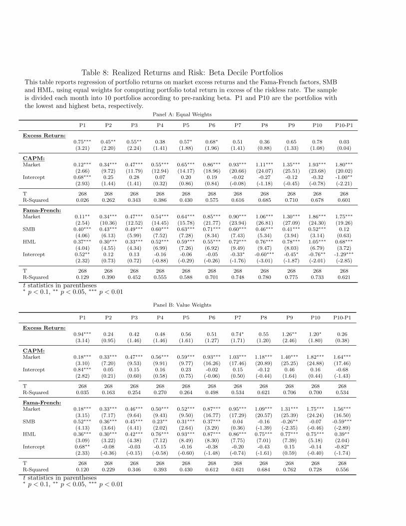
Table 8: Realized Returns and Risk: Beta Decile PortfoliosThis table reports regression of portfolio returns on market excess returns and the Fama-French factors, SMBand HML, using equal weights for computing portfolio total return in excess of the riskless rate. The sampleis divided each month into 10 portfolios according to pre-ranking beta. P1 and P10 are the portfolios withthe lowest and highest beta, respectively.