THE IMPACT OF EXCHANGE RATE DEPRECIATION AND THE MONEY ... · The Impact of Exchange Rate...

391The Impact of Exchange Rate Depreciation and the Money Supply Growth on Inflation:the Implementation of the Threshold Model

THE IMPACT OF EXCHANGE RATE DEPRECIATION ANDTHE MONEY SUPPLY GROWTH ON INFLATION:

THE IMPLEMENTATION OF THE THRESHOLD MODEL1

Rizki E. Wimanda 2

This paper investigates the impact of exchange rate depreciation and money growth to the CPI

inflation in Indonesia. Using monthly data from 1980:1 to 2008:12, our econometric evidence shows that

there are indeed threshold effects of money growth on inflation, but no threshold effect of exchange rate

depreciation on inflation. However the threshold value for exchange rate depreciation is found at 8.4%,

and there is no significant difference between the coefficient both below and above the threshold value.

Meanwhile, two threshold values are found for money growth, i.e. 7.1% and 9.8%, and they are statistically

different. The impact on inflation is high when money grows by up to 7.1%, it is moderate when money

grows by 7.1% to 9.8%, and it is low when money grows by above 9.8%.

JEL Classification: C22; E31; E51.

Keywords: Inflation, Threshold Effect; Indonesia

1 Extracted from Wimanda (2010), Doctoral Thesis, Chapter 4, ≈Threshold Effects of Exchange Rate and Money Growth on Inflation∆.2 Researcher in Economy at Bank Indonesia, email: [email protected].

Abstract

392 Bulletin of Monetary, Economics and Banking, April 2011

I. INTRODUCTION

Concerns about inflation have been very intense since Indonesia adopted the inflation

targeting in 2000. One of the important topics of the study is to examine the factors that cause

inflation.

Wimanda (2010)3 found that inflation in Indonesia is significantly influenced by inflation

expectations (backward-looking and forward-looking), output gap, exchange rate depreciation,

and growth in money supply. Analysis of monthly samples from early 1980 until the end of

2008 shows that the formation of inflation expectations in Indonesia is still dominated by the

backward-looking inflation expectations with a share of 0.7, while the portion of forward-

looking inflation expectations is around 0.2. In his analysis,nWimanda also found that the

impact of exchange rate is greater than the impact from the growth in money supply (M1). The

analysis assumes that the impact of these two variables is linear, meaning that their impact is

constant for each level of exchange rate depreciation and money supply growth.

By using the threshold model, this paper will test whether the impact of exchange rate

and money supply growth on inflation is linear or not. And then to test whether there is a

threshold value, how much the threshold value that can be identified, and the extent of the

impact.

The systematic of this paper is as follows. Literature study will be discussed in the second

chapter. Methodology and data will be discussed at the third part of this paper, while the

estimation results and conclusions will be presented at the fourth and fifth chapter.

II. THEORY

2.1. Pass-through of Exchange Rate

One of the central issues in international economics is the pass-through of exchange rate

which is defined as an impact of 1 percent of depreciation on the domestic inflation. In general,

to test the exchange rate pass-through, we estimate at the following equation:

3 In the 3rd chapter of Doctoral Thesis, ≈Determinants of Inflation and The Shape of Phillips Curve∆.

(1)πt = α + γe

t + δx

t + ε

t

where is the domestic inflation, is the depreciation of the exchange rate (nominal), and is the

other control variables (in growth).

In general, the study of exchange rate pass-through can be divided into 3 groups.


The first group is the study of the impact of exchange rate on the import prices of certain

industries, like as conducted by Bernhofen and Xu (1999) and Goldberg (1995). The second

group is the study the impact of exchange rate on import prices in the aggregate, for

example Hooper and Mann (1989) and Campa and Goldberg (2005). And the third group

is the study of the impact of exchange rate on the CPI or WPI, for example, Papell (1994)

and McCarthy (2000).

Although the literature on exchange rate pass-through is very plentiful, but empirical

studies mostly focus on developed countries. A survey carried out by Menon (1995) showed

that 48 studies on exchange rate pass-through specifically cover the United States and Japan.

Similarly, Goldberg and Knetter (1997) mentioned that the study of exchange rate pass-through

during the 1980s is dominated by the USA.

For OECD countries, the study of the impact of exchange rate pass-through on their

import prices was conducted by Campa and Goldberg (2005). They found that exchange rate

pass-through is partial, where import prices reflect 60 percent of exchange rate movements in

the short term and nearly 80 percent in the long term. They also found that countries which

have a low exchange rate volatility and low inflation have a low impact of exchange rates pass-

through.

Using 71 countries data from 1979 to 2000, Choudhri and Hakura (2006) showed that

there was a strong positive relationship between the exchange rate pass-through with the

inflation average. Countries with low inflation tend to have a low exchange rates pass-through,

and vice versa.

The relationship of exchange rate and inflation in Malaysia, Philippines, and Singapore

was examined by Alba and Papper (1998) during the Q1 of 1979 Q1 until the Q2 of 1995. They

found that the exchange rate pass-through for the Philippines is higher compared to Malaysia,

while the exchange rate pass-through to Singapore was oppositely negative.

To support the argument of ≈fear of floating∆, Calvo and Reinhart (2000) also examined

a number of developed and developing countries, including Malaysia and Indonesia. By using

the monthly data from August 1997 through November 1999, they found the pass-through

rate in Indonesia was 0.062.

2.2. Relationship between Money and Inflation

The quantity theory and the exchange equation provide a useful framework to analyze

empirically the relevance of money in the economy. The relationship of money and inflation can


be derived from the money demand equation. The public wants to hold money to buy goods

and services. If the price of goods and services rises, people tend to hold more money. The most

important factor in the demand for money is the income. When incomes rise, people will tend

to shop more. Higher expenditures are associated with more cash on hand. Thus, this relationship

can be written as:

where M is the nominal money, P is the price level based on the CPI or GDP deflator, Y is the

income and k is the proportion factor. Equation (2) can be rewritten as

(3)

By assuming that the causality from M to P exists, equation (3) states that the quantity of

money determines the price level, although money is not the only factor. For example, when

income and other factors which are reflected by k do not change, and when the quantity of

money increases, the price level will increase.

Milton Friedman (1968) argues that inflation is a monetary phenomenon. Studies

conducted by Lucas (1980), Dwyer and Hafer (1988), Friedman (1992), Barro (1993), McCandless

and Weber (1995), Dewald (1998), Rolnick and Weber (1997) and others concluded that the

changes in the quantity of money and price changes have a close relationship.

Dwyer and Hafer (1999) showed that the price level has a positive and proportional

relationship to the quantity of money in America, Britain, Japan, Brazil, and Chile during the

20th century. They also showed that in the shorter term, 5 years, the relationship of money

growth and inflation remains in force.

Empirical study of the relationship between money growth (M1 and M2) and the inflation

in 160 countries was carried out by De Grauwe and Polan (2005). They showed that during the

past 30 years, the relationship of money supply growth and inflation is still valid. However, after

dividing the sample based on the rate of inflation, they showed that countries with low inflation

(below 10%), the relationship between both variables weakened. Conversely, the relationship

was strong in the countries with high inflation rates. However, this study did not specify at

what level of money supply will give a different effect on inflation.

(2)= k Y,ΜP

=P1k

ΜY


2.3. Threshold Model Application

Threshold model is a special case of complex statistical frameworks, such as mixture

models, switching models, Markov-switching model, and smooth transition threshold model

(Hansen, 1997).

Threshold model can be applied in many cases. For example, Galbraith (1996) conducted

a study on the relationship betweennmoney and output. By using the data of US and Canada,

he found that money has a strong influence on the output when the value of money growth is

below certain threshold. This result is consistent with the proposition that the monetary policy

has little impact or no impact at all on when the money growth is very high.

Khan and Senhadji (2001) investigated the relationshipnbetween the inflation

andneconomic growth in 140 countries during the period of 1960 untiln1998. They argue

thatninflation has a negative impact on the economy when inflation is above certain threshold

values. In contrast, inflation has a positive impact on the economy when inflation is below the

threshold value. They found that the threshold value for developed countries is 1-3 percent,

and about 11-12 percent of threshold value for developing countries.

Threshold model is also used by Papageorgiou (2002) to evaluate the level of openness

of the economy. Foster (2006) examined the relationship of export and economic growth for

African countries. The evaluation of the fiscal deficit was also performed using the threshold

models, for example for the case of USA (see Arestis, Cipollini and Fattouh, 2004) and Spain

(see Bajo-Rubio, Diaz-Roldan and Esteve, 2004).

Meanwhile, the study of the threshold of exchange to the inflation and the threshold of

money supply to inflation, to our knowledge, does not yet exist. Therefore, this study is conducted

with the intention to complete the literature gap.

III. METHODOLOGY

3.1. Empirical Model and the Estimation Technique

This study is using the threshold modelnto answer the questions above. Threshold model

is a special case of a complex statistical framework, such as mixture models, switching models,

Markov-switching models, and smooth transition threshold models. In general, the threshold

model can be written as follows:

(4)yt = β‘

j x

t + δ

1z

tI (th

t < λ) + δ

2 z

t I (th

t > λ) + µ

t


where is the dependent variable, is the explanatory variable to be tested, is the vector of other

explanatorynvariables, is the indicator function, is a threshold variable, and is the value of the

threshold. In the equation above, the observations are divided into two regimes; depend on

whether the threshold variable is smaller or larger than the value of.

To estimate the model, the threshold value and the value of slope parameter are estimated

simultaneously. Hansen (1997) recommended seeking estimates of by finding the minimum

valuenof sum of squared errors. To ensure that the number of observations in each regime is

sufficient, the models are estimated for all the threshold value from the variable threshold

between the 10th and 90th percentile.

Having found the threshold value, we need to test whether the value is statistically

significant or not. In this case, whether the null hypothesis is to be rejected or accepted. One

thing that may complicate is the non- identified threshold value in the null hypothesis. This

implies that the classical test does not have a standard distribution, so that critical values cannot

be obtained from the standard distribution tables.

This study follows Hansen (1997, 2000) in the search for multiple regimes in the data by

using the exchange rate depreciation and the growth of M1 as the threshold variable. This

method, which is based on the asymptotic distribution, will test the significance of regimes

selected by the data.

In this study, we do not evaluate long-term relationship of the value of the exchange rate

and the money supply to the price level, but we are more interested to see the short-term

relationship of the exchange rate depreciation and the money supply growth to inflation. To

examine the existence of a threshold effect of exchange rate depreciation on inflation, this

hybrid model of Phillips curve will be estimated as follows:

where,

is inflation, πt - 1

is the backward-looking inflation expectations, πt + 1

is the forward-looking

inflation expectations, gapt is the output gap, er

t is the depreciation of the exchange rate4, er*

(5)

πt = c + α

1π

t - 1 + α

2π

t + 1 +

βgap

t + γ

1(1 - d

t ) [(er

t)I (er

t > er*)] +

γ2d

t [(er

t)I (er

t < er*)] + θm

t + δ

1crisis + δ

2 fuel + δ

3 fitri + ε

t

e

4 The exchange rate is defined as the domestic currency per foreign currency. In this case we use Rp/USD. Thus, a negative er valuemeans depreciation, while a positive er value indicates an appreciation

e


is the threshold value of the exchange rate, mt is the growth ofnmoney supply (M1), crisis is

the dummy variable to capture the financial crisis 1997-1998, fuel is a dummy variable to

capture the fuel price surge in January 2005 and October 2005, and fitri is the dummy variable

to capture the phenomenon of Idul Fitri.

We use instrumental variables (IV) estimators, which is the two-stage leastnsquares (TSLS).

Thisnestimation methodncan overcome the endogeneity problems given that within the model

used there is theninflation value in the future.

Model estimation is done by conditional least squares method which can be explained as

follows:

For each threshold value ert*, the model is estimated through TSLS, to obtain the sum of

squared residuals (SSR). The least squares estimation of ert* is obtained by choosing the threshold

value ert* which has the minimum value of SSR. If we put all the threshold value observations

into the vector, the compact notation of equation (2) then is as follows:

Once the threshold value is obtained, we need to examine whether the threshold effect

is statistically significant or not. In equation (2), to test the existence of the threshold effect, we

need to test the null hypothesis, which is H0 : γ

1 = γ

2. Hansen (1997, 2000) suggested the

bootstrap method to simulate the asymptotic distribution of the likelihood ratio test from the

H0 as the following:

(6)y = xβ

er + ε , er = er,....er ,

er* = argmin [ S

1(er), er = er,....,er ] (7)

where βer

= ( c α

1 α

2 β γ

1 γ

2 θ δ

1 δ

2 δ

3 )’ is the vector of parameters, y is the dependent variable,

and x is the matrix of the explanatory variables. It is noteworthy that the coefficient vector β is

indexed with er to show its dependence to the threshold value, which ranged from er to er. We

define S1 (er) as SSR with the threshold value of exchange rate depreciation on er. The threshold

estimation value er* which is obtained is the threshold value with the minimum S1 (er) value,

namely:


where S0 and S

1 is the SSR for H

0 : γ

1 = γ

2 and H

1 : γ

1 = γ

2. In other words, S

0 and S

1 is the SSR from

the equation (2) without and with the threshold effects. Asymptotic distribution of LR0 is non-

standard and dominate the distribution of χ2. The distribution of generally depends on the

moments of sample, so that the critical values cannot be tabulated.

Given that γ has not been identified, the asymptotic distribution of LR0 is not χ2 .

Hansen (1997) showed that this can be approximated by using the following bootstrap

procedure:

1. Set µt* , t = 1,....,n as random number, drawn from a normal distribution whose mean is zero

and whose variance is one i.e. N (0,1).

2. Set yt* = µ

t*.

3. By using the observation of xt, t = 1,....,n, regress y

t* at x

t and find the residual variance

from the linear model, where.

4. By using the observation of xt, t = 1,....,n, regress y

t* at x

t ( γ ) and find thenresidual variance

from the threshold model, where

and γ are the threshold value.

5. Calculate .

6. Repeat step number 4 and 5 for the other γ.

7. Find .

8. Repeat step 1 to 7 over and over again.

Hansen (1997) also showed that the repetitive sampling from Fn∗ can be used as an

approximation to the asymptotic distribution from Fn. The p-value of this test is to

calculate the percentage of bootstrap samples whose the value of Fn∗ exceeds LR

0 (see

equation (5)).

LR0 = n ,

(S0 - S

1)

S1

(8)

σn∗2∼

σn∗2∼

(γ)


where S1(er) and S

1(er*) is the SSR from equation (2) with threshold er and er*. Define c

ξ (β )

as the β-level critical value for ξ from Table 1 in Hansen (2000). Thus that defines

Hansen (2000) shows that is asymptotically valid for β-level confidence at er. To get

a confidence interval, we plot the likelihood ratio LR(er) with the threshold value (er), pull

a straight line on cξ (β ), and mark the threshold value with the likelihood ratio whose

value is under the critical value. It should be noted that the LR(er) will be equal to zero

when er = er*.

To test the existence of threshold effect of the money growth toward inflation, we use

the same model, but we replace the exchange rate depreciation with the growth of money

supply as the threshold variable. The model will be next estimated as follows:

πt = c + α

1π

t - 1 + α

2π

t + 1 +

βgap

t + γer

t + θ

1(1 - d

t ) [(m

t ) I (m

t > m*)]

+ θ2d

t [(m

t)I (m

t < m*)] + δ

1crisis + δ

2 fuel + δ

3 fitri + ε

t

e

(11)

where .

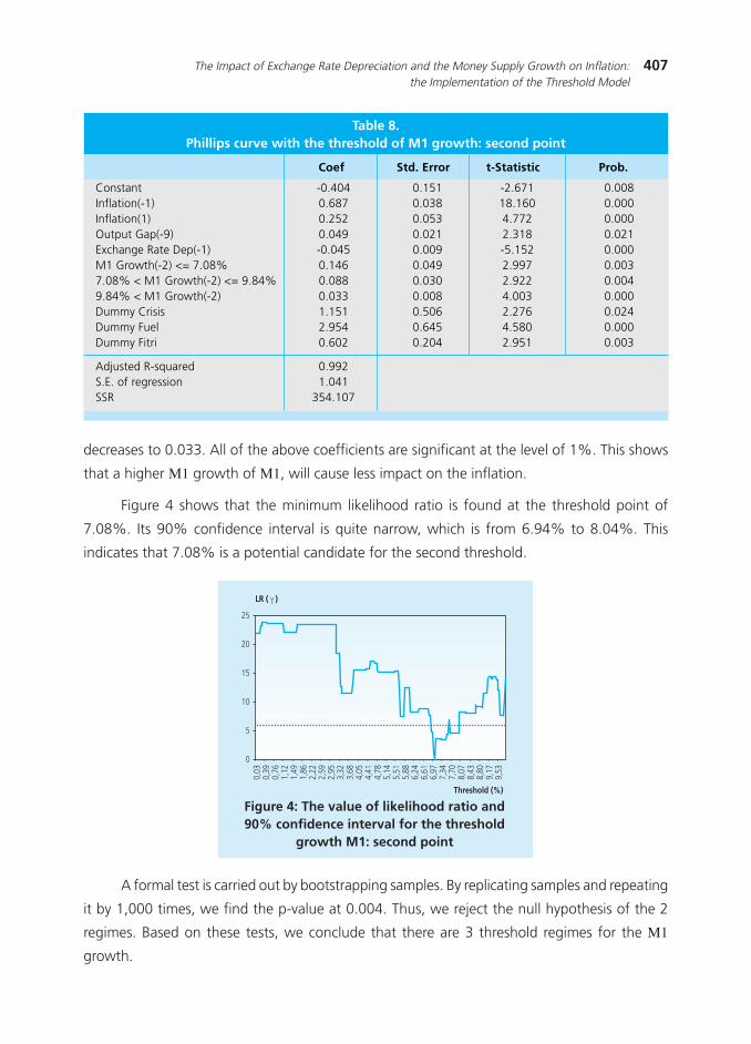
Meanwhile the estimation and testing procedures for threshold growth of money supply

is the same as the procedure above.

3.2. Data

We use CPI data, output gap, exchange rate, and M1. These data is obtained from

Bank Indonesia (BI) and BPS. For the analysis, we use the monthly data from 1980 to 2008

(see Table 1).

This study follows Hansen (2000) in forming the confidencenregionnfor er*. The confidence

intervalsnfor the threshold parameter inversion are built by inversing the asymptotic distribution

of the likelihood ratio statistics. In this case, we tested null hypothesis H0 : er* = er by calculating

the likelihood test as follows:

(9)LR(er) = n ,S

1(er) - S

1(er*)

S1(er*)

(10)Γ = [er : LR(er) < cξ (β )]


IV. RESULT AND ANALYSIS

4.1. Threshold Effect on the Exchange Rate Depreciation

Table 3 below shows the results of TSLS estimation of the equation (2) without the presence

of threshold effect (by setting γ1 = γ

2). From this table we can see that all the parameters are

significant, except for constant. By using the adjusted HP filter as a proxy in the calculation

ofnpotential output, we find that the coefficient of exchange rate depreciation (yoy) is -0.050

and the coefficient of M1 growth is 0.021. These resultnshows that in average the impact of

exchange rate depreciation on inflation is still greater than the impact of the money supply

growth.

Table 1. Data

NoNoNoNoNo D a t aD a t aD a t aD a t aD a t a FrequencyFrequencyFrequencyFrequencyFrequency PeriodPeriodPeriodPeriodPeriod SourceSourceSourceSourceSource

1 CPI Inflation Monthly 1980:1 to 2008:12 BPS and BI2 Output gap Monthly 1980:1 to 2008:12 Author3 Exchange rate Monthly 1980:1 to 2008:12 BI4 M1 Monthly 1980:1 to 2008:12 BI

Table 2.Descriptive statistic of the data (year-on-year)

1980 - 19971980 - 19971980 - 19971980 - 19971980 - 1997

CPI Inflation 9.01 3.37 57.59 23.28 10.52 9.52Exchange Rate Depreciation -6.63 10.67 -67.97 13.04 1.32 18.91M1 Growth 19.53 11.52 29.17 9.02 17.70 6.39Output Gap - HPA 0.19 3.39 -11.76 1.97 -2.31 3.25Output Gap - Peak-to-Peak -2.50 1.54 -13.13 2.03 -5.20 3.29

D a t aD a t aD a t aD a t aD a t a 19981998199819981998 1999 - 20081999 - 20081999 - 20081999 - 20081999 - 2008

MeanMeanMeanMeanMean Std DevStd DevStd DevStd DevStd Dev MeanMeanMeanMeanMean Std DevStd DevStd DevStd DevStd Dev MeanMeanMeanMeanMean Std DevStd DevStd DevStd DevStd Dev

Table 1: Robustness check for Phillips curve with the threshold of exchange rate

depreciation

Table 3.Phillips Curve without Threshold

Constant -0.148 0.141 -1.051 0.294Inflation (-1)0.710 0.042 17.078 0.000Inflation(1) 0.225 0.058 3.911 0.000Output Gap (-9) 0.062 0.023 2.703 0.007Exchange Rate Dep(-1) -0.050 0.009 -5.223 0.000M1 Growth(-2) 0.024 0.007 3.261 0.001Dummy Crisis 1.293 0.539 2.400 0.017Dummy Fuel 2.940 0.676 4.349 0.000Dummy Fitri 0.548 0.213 2.567 0.011

Adjusted R-squared 0.991S.E. of regression 1.093SSR 393.024

Coef Std. Error t-Statistic Prob.


Tabel 4.Phillips Curve with The Threshold of Exchange Rate Depreciation

Constant -0.169 0.144 -1.179 0.239Inflation(-1) 0.719 0.045 16.071 0.000Inflation(1) 0.211 0.062 3.382 0.001Output Gap(-9) 0.064 0.024 2.703 0.007Exchange Rate Dep(-1) <= -8.4% -0.056 0.012 -4.652 0.000-8.4% > Exchange Rate Dep(-1) -0.045 0.010 -4.567 0.000M1 Growth(-2) 0.026 0.008 3.294 0.001Dummy Crisis 1.154 0.547 2.109 0.036Dummy Fuel 2.973 0.693 4.293 0.000Dummy Fitri 0.548 0.218 2.516 0.012



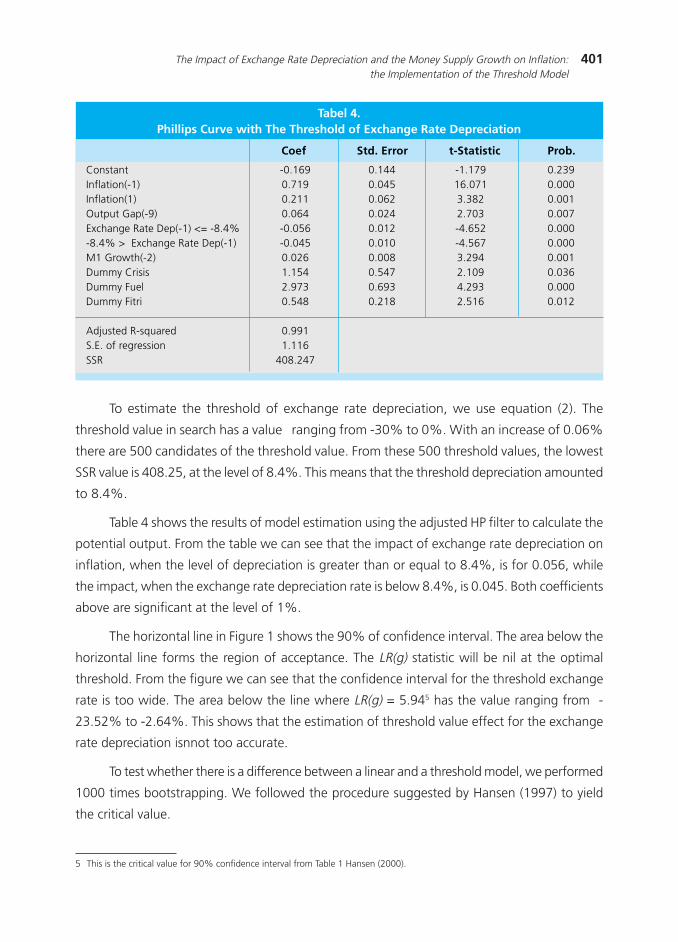
To estimate the threshold of exchange rate depreciation, we use equation (2). The

threshold value in search has a value ranging from -30% to 0%. With an increase of 0.06%

there are 500 candidates of the threshold value. From these 500 threshold values, the lowest

SSR value is 408.25, at the level of 8.4%. This means that the threshold depreciation amounted

to 8.4%.

Table 4 shows the results of model estimation using the adjusted HP filter to calculate the

potential output. From the table we can see that the impact of exchange rate depreciation on

inflation, when the level of depreciation is greater than or equal to 8.4%, is for 0.056, while

the impact, when the exchange rate depreciation rate is below 8.4%, is 0.045. Both coefficients

above are significant at the level of 1%.

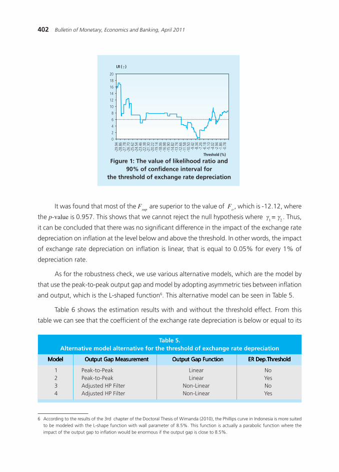
The horizontal line in Figure 1 shows the 90% of confidence interval. The area below the

horizontal line forms the region of acceptance. The LR(g) statistic will be nil at the optimal

threshold. From the figure we can see that the confidence interval for the threshold exchange

rate is too wide. The area below the line where LR(g) = 5.945 has the value ranging from -

23.52% to -2.64%. This shows that the estimation of threshold value effect for the exchange

rate depreciation isnnot too accurate.

To test whether there is a difference between a linear and a threshold model, we performed

1000 times bootstrapping. We followed the procedure suggested by Hansen (1997) to yield

the critical value.

5 This is the critical value for 90% confidence interval from Table 1 Hansen (2000).


Figure 1: The value of likelihood ratio and90% of confidence interval for

the threshold of exchange rate depreciation

Threshold (%)

LR ( γ )

0

2

4

6

8

10

12

14

16

18

20

-29.

94-2

8.86

-27.

78-2

6.70

-25.

62-2

4.54

-23.

46-2

2.38

-21.

30-2

0.22

-19.

14-1

8.06

-16.

98-1

5.90

-14.

82-1

3.74

-12.

66-1

1.58

-10.

50-9

.42

-8.3

4-7

.26

-6.1

8-5

.10

-4.0

2-2

.94

-1.8

6-0

.78

Table 5.Alternative model alternative for the threshold of exchange rate depreciation

ModelModelModelModelModel Output Gap MeasurementOutput Gap MeasurementOutput Gap MeasurementOutput Gap MeasurementOutput Gap Measurement Output Gap FunctionOutput Gap FunctionOutput Gap FunctionOutput Gap FunctionOutput Gap Function ER Dep.ThresholdER Dep.ThresholdER Dep.ThresholdER Dep.ThresholdER Dep.Threshold

1 Peak-to-Peak Linear No2 Peak-to-Peak Linear Yes3 Adjusted HP Filter Non-Linear No4 Adjusted HP Filter Non-Linear Yes

It was found that most of the Fsup

are superior to the value of Fo , which is -12.12, where

the p-value is 0.957. This shows that we cannot reject the null hypothesis where γ1 = γ

2 . Thus,

it can be concluded that there was no significant difference in the impact of the exchange rate

depreciation on inflation at the level below and above the threshold. In other words, the impact

of exchange rate depreciation on inflation is linear, that is equal to 0.05% for every 1% of

depreciation rate.

As for the robustness check, we use various alternative models, which are the model by

that use the peak-to-peak output gap and model by adopting asymmetric ties between inflation

and output, which is the L-shaped function6. This alternative model can be seen in Table 5.

Table 6 shows the estimation results with and without the threshold effect. From this

table we can see that the coefficient of the exchange rate depreciation is below or equal to its

6 According to the results of the 3rd chapter of the Doctoral Thesis of Wimanda (2010), the Phillips curve in Indonesia is more suitedto be modeled with the L-shape function with wall parameter of 8.5%. This function is actually a parabolic function where theimpact of the output gap to inflation would be enormous if the output gap is close to 8.5%.


Table 6.Robustness check for Phillips curve with the threshold of exchange rate depreciation

Variable Model-1 Model-2 Model-3 Model-4

Constant 0.007 0.011 -0.325*** -0.358***(0.186) (0.192) (0.122) (0.127)

Inflation (-1) 0.714*** 0.730*** 0.694*** 0.705***(0.043) (0.048) (0.037) (0.041)

Inflation(1) 0.223*** 0.199*** 0.249*** 0.233***(0.059) (0.067) (0.051) (0.056)

Output Gap Linear (-9) 0.071** 0.081**(0.03) (0.032)

Output Gap Non-Linear(-9) 0.0003** 0.0004**(0.00016) (0.00017)

Exchange Rate Dep(-1) -0.048*** -0.047***(0.009) (0.009)

Exchange Rate Dep(-1) <= Threshold -0.057*** -0.054***(0.013) (0.011)

Threshold < Exchange Rate Dep(-1) -0.041*** -0.041***(0.009) (0.009)

M1 Growth(-2) 0.027*** 0.030*** 0.027*** 0.031***(0.008) (0.009) (0.008) (0.008)

Dummy Crisis 1.228** 1.154** 0.652 0.462(0.536) (0.547) (0.405) (0.422)

Dummy Fuel 2.944*** 2.973*** 2.772*** 2.805***(0.683) (0.693) (0.648) (0.665)

Dummy Fitri 0.551** 0.548** 0.554*** 0.554***(0.215) (0.218) (0.208) (0.213)

Adjusted R-squared 0.991 0.991 0.992 0.991S.E. of regression 1.103 1.116 1.066 1.091SSR 400.161 408.247 373.986 390.569

Threshold ER -8.40 -8.40

p-value 0.999 0.966

Remarks:- The number between parentheses is the error standard.- ***, **, and * indicate the significance level at the level of 1%, 5%, and 10%.

threshold value (γ1 ). And above its threshold value in model 2 and model 4 (γ

2 ) the value is

negative and significant. We found that the threshold value is equal to the threshold value on

the previous model, at the level of -8.4%. Coefficient value γ1 of is in the range of -0.054 to -

0.057, while the coefficient value of γ2 is relatively the same at -0.041.

After performing as much as 1,000 times bootstrapping, model 2 and model 4 yield the

same conclusion with the main model. Overall, from the bootstrap test statistics, there is not

any statistical significance on these variables. The p-values range between 0966 and 0999.

This implies that there is no significant difference between the impact of exchange rate

depreciation on inflation, above and below its threshold value.


If we compare model 1 and model 2, as well as model 3 and model 4, we can see that

the value of SSR for the threshold model is greater than the value of the SSR on the linear

model. This confirms the above conclusion.

Figure 2.The impact of exchange ratedepreciation on the inflation: an illustration

Figure 2 above illustrates the impact of exchange rate depreciation on inflation. From this

picture, we can see that the slope in solid blue line is the same for every point. This linear

impact (solid blue line) is more preferable than the non-linear impact of (dashed brown line).

4.2 Threshold Effect on the Money Growth

To estimate the threshold valuenfor the moneynsupply growth, we use equation (8) with

the output gap, which is calculated based on thenadjusted HP filter. This search for the threshold

value starts from 0% to 40%, with an increase of 0.08. This means that there are approximately

500 candidates for the threshold value. We found that the threshold value for the M1 growth

was 9.84%7.

Table 7 shows thenestimation results of threshold with using the adjusted HP filter as a

measurement of the output gap. Given that the results of the main variables are quite robust,

that all coefficients are statistically significant, we can then immediately analyze its threshold

results. From the table, the coefficient of the money supply growth, below or equal to 9.84%

( θ1 ), is 0.099, while the coefficient of the money supply growth above 9.84% ( θ

2 ) is 0.032.

Both coefficients are significant at the level of 1%.

Inflation (%)

0

0,2

0,4

0,6

0,8

1

1,2

1,4

ER (%)-8.4

-25,0 -23,8 -22,5 -21,3 -20,0 -18,8 -17,5 -16,3 -15,0 -13,8 -12,5 -11,3 -10,0 -8,8 -7,5 -6,3 -5,0 -3,8 -2,5 -1,3 0,0

7 This value give the smallest SSR.


This result impliesnthat there are differences in the impact of the M1 growthnon

inflation,nabove or below its threshold value at 9.84%. As an illustration, shall M1 grow by 5%

this month, and then there will be an additional inflation of 0.5% in two months to come.

Meanwhile, shall M1 grow 10% this month; there will be then an additional average inflation

of 0.98% within 2 months.

Table 7.Phillips curve with the threshold of M1 growth: first point

Constant -0.361 0.150 -2.405 0.017Inflation(-1) 0.695 0.039 17.947 0.000Inflation(1) 0.241 0.054 4.468 0.000Output Gap(-9) 0.053 0.022 2.455 0.015Exchange Rate Dep(-1) -0.047 0.009 -5.257 0.000M1 Growth(-2) <= 9.84% 0.099 0.030 3.341 0.0019.84% < M1 Growth(-2) 0.032 0.008 3.877 0.000Dummy Crisis 1.229 0.516 2.384 0.018Dummy Fuel 2.983 0.656 4.549 0.000Dummy Fitri 0.583 0.207 2.821 0.005



Figure 3: The value of likelihood ratio and90% confidence interval for the threshold

of M1 growth: first point

Once the threshold value is identified, the next important question is how accurate are

these estimates. This requires the calculation of the confidence regions around the threshold

value. Figure 3 illustrates the value of likelihood ratio and the threshold value, as well as 90%

LR ( γ )

0

5

10

15

20

25

30

35

40

45

0,08

1,68

3,28

4,88

6,48

8,08

9,68

11,2

812

,88

14,4

816

,08

17,6

819

,28

20,8

822

,48

24,0

825

,68

27,2

828

,88

30,4

832

,08

33,6

835

,28

36,8

838

,48

Threshold (%)


confidence intervals. As explained above, the confidence region is calculated by taking the

values of M1 growth where the value of LR(M1) is below the horizontal line. From this figure

it shows that the confidence interval for the money growth is quite narrow, around 7.12% -

10%. This indicates that the estimated threshold value is accurate enough.

The next step is to test whether the threshold value exists by performing bootstrapping.

By generating new samples, repeated by 1,000 times for the percentile estimation of the

asymptotic null distribution Fn*, we find that the p-value is 0.001. Thus, the null hypothesis

(linear model) can be rejected and it concludes that there is a threshold value for the M1

growth.

After finding the first threshold value, we seek the possibility of another threshold value.

We can find three regimes at the same time, but this would be very inefficient in terms of

computation time. Chong (1994) and Bai (1997) showed that the sequential estimation is

consistent, so that it can avoid the problem of calculation. This means that we can fix the first

threshold figure, en then seek the second one by assuming that the first threshold is already

fixed.

After finding the first threshold value, we seek the possibility of another threshold value.

We can find three regimes at the same time, but this way is very inefficient in terms of

computation time. Chong (1994) and Bai (1997) showed that the sequential estimation is

consistent, so that it can avoid the problem of calculation. This means we can make the fix-it

figures that the first threshold then seek a second threshold value by assuming that the first

threshold has been fixed.

We begin by considering the possibility of another threshold value between 9.84% and

40%. With a value addition by 0.075 there are 400 candidates for the threshold value. It is

found that the smallest SSR is when the threshold is at 17.13%. This means that 17.3% is the

second threshold candidate. TSLS estimation results can be seen in Table A (see Appendix).

Although these entire M1 growth coefficients are significant at level of 1%, but after conducting

the bootstrapping, we found the p-value at 0.177 which is slightly larger than 10%. Thus, the

null hypothesis from these 2 threshold regime cannot be rejected. In other words, the relationship

between inflation and the M1 growth is linear by the time M1 grows above 9.84%.

The next effort to search the threshold candidate is between 0% and 9.84%. We selected

350 values and found the minimum SSR at the point of 7.08%. TSLS Estimation results with

2 thresholds: 9.84% and 7:08% can be seen in Table 8. From the table we can note that the

coefficient of M1 growth, when it grows under 7.08%, is 0.146; when it grows between

7.08% and 9.84%, the coefficient is 0.088, and when it grows over than 9.84%, the coefficient


decreases to 0.033. All of the above coefficients are significant at the level of 1%. This shows

that a higher M1 growth of M1, will cause less impact on the inflation.

Figure 4 shows that the minimum likelihood ratio is found at the threshold point of

7.08%. Its 90% confidence interval is quite narrow, which is from 6.94% to 8.04%. This

indicates that 7.08% is a potential candidate for the second threshold.

Table 8.Phillips curve with the threshold of M1 growth: second point

Constant -0.404 0.151 -2.671 0.008Inflation(-1) 0.687 0.038 18.160 0.000Inflation(1) 0.252 0.053 4.772 0.000Output Gap(-9) 0.049 0.021 2.318 0.021Exchange Rate Dep(-1) -0.045 0.009 -5.152 0.000M1 Growth(-2) <= 7.08% 0.146 0.049 2.997 0.0037.08% < M1 Growth(-2) <= 9.84% 0.088 0.030 2.922 0.0049.84% < M1 Growth(-2) 0.033 0.008 4.003 0.000Dummy Crisis 1.151 0.506 2.276 0.024Dummy Fuel 2.954 0.645 4.580 0.000Dummy Fitri 0.602 0.204 2.951 0.003



Figure 4: The value of likelihood ratio and90% confidence interval for the threshold

growth M1: second point

Threshold (%)

0

5

10

15

20

25

LR ( γ )

0,03

0,39

0,76

1,12

1,49

1,86

2,22

2,59

2,95

3,32

3,68

4,05

4,41

4,78

5,14

5,51

5,88

6,24

6,61

6,97

7,34

7,70

8,07

8,43

8,80

9,17

9,53

A formal test is carried out by bootstrapping samples. By replicating samples and repeating

it by 1,000 times, we find the p-value at 0.004. Thus, we reject the null hypothesis of the 2

regimes. Based on these tests, we conclude that there are 3 threshold regimes for the M1

growth.


Next we look for another threshold value candidate between 0% and 7.08%. With an

addition of 0.028%, we evaluated 250 candidates. Of the 250 these candidates, we found

that the SSR value is the lowest at the point of 4.93%.

Table B (see Appendix) presents the TSLS estimation result with four regimes. All

coefficients are significant, except the coefficient for M1 growth from 0% to 4.93% ( p-value

= 0273 ). The formal testing through bootstrapping produces p-value by 0.191. This indicates

that the relationship of inflation with the M1 growth is linear when M1 grows between 0%

and 7.12%. Given that the third threshold is not significant, it is impossible to separate

further the samples.

Table 9.Alternative model for the threshold of M1 growth

Model Output Gap Measurement Output Gap Function M1 Threshold

5 Peak-to-Peak Linear No6 Peak-to-Peak Linear Yes7 Adjusted HP Filter Non-Linear No8 Adjusted HP Filter Non-Linear Yes

As for robustness check, again we use a variety of models with the difference that lies in

the measurement of the output gap and the non-linear Phillips curve. Table 9 shows the

difference.

As shown in Table 10, these empirical results yield some interesting results. First, all

coefficients, except the constant and dummy variables for the crisis on some models, are

significant. Second, the estimation of the threshold value is the same, 9.84% and 7.08%.

Third, the coefficient of the threshold effect is somewhat different, yet the difference is

abysmal. The coefficient of M1 growth when growing under 7.08% ranges from 0.156 to

0.160; coefficient of M1 growth when growing between 7.08% and 9.84% ranges from

0.094 to 0.096, and the coefficient of M1 growth when growing over 9.84% ranges from

0.035 to -0037.

Given that all the p-values of the bootstrapping are less than 1%, then we can reject

the null hypothesis for the two regimes and prefer to the three regimes. In addition, when

compared to the SSR value to the threshold model (model 6 and model 8) and the SSR value

on the linear model (model 5 and model 7), we found that the threshold model is better than

the linear model.


Table 10:Robustness check for the threshold of M1 growth

Variable Model-1 Model-2 Model-3 Model-4

Constant 0.062 -0.284 -0.279** -0.559***(0.187) (0.183) (0.12) (0.137)

Inflation (-1)0.714*** 0.689*** 0.694*** 0.672***(0.043) (0.039) (0.037) (0.034)

Inflation(1) 0.223*** 0.250*** 0.251*** 0.273***(0.059) (0.053) (0.051) (0.047)

Output Gap Linear(-9) 0.074** 0.060**(0.03) (0.028)

Output Gap Non-Linear(-9) 0.000334** 0.00033**(0.000161) (0.000153)

Exchange Rate Dep(-1) -0.048*** -0.043*** -0.047*** -0.042***(0.009) (0.008) (0.009) (0.008)

M1 Growth(-2) 0.024*** 0.026***(0.007) (0.007)

M1 Growth(-2) <= 2nd Threshold 0.156*** 0.160***(0.049) (0.048)

2nd Threshold < M1 Growth(-2) <= 1st Threshold 0.096*** 0.094***(0.031) (0.03)

1st Threshold < M1 Growth(-2) 0.035*** 0.037***(0.008) (0.008)

Dummy Crisis 1.235** 1.122** 0.644 0.633(0.539) (0.503) (0.406) (0.386)

Dummy Fuel 2.929*** 2.968*** 2.752*** 2.819***(0.685) (0.65) (0.649) (0.619)

Dummy Fitri 0.550** 0.608*** 0.553*** 0.611***(0.216) (0.205) (0.209) (0.199)

Adjusted R-squared 0.991 0.992 0.992 0.992S.E. of regression 1.107 1.045 1.070 1.014SSR 403.146 357.419 376.347 336.461

1st Threshold 9.84 9.842nd Threshold 7.08 7.08

p-value 0.005 0.005

Remarks:- The number within the parentheses is the error standard.- ***, **, and * indicates the significance level on the level of 1%, 5%, and 10%.

From the test results and analysis above, these empirical results provide strong evidence

that the relationship of M1 growth and inflation can be described by three regimes. Figure

5 illustrates this relationship. From the picture, we can see that the slope of the solid

brown line when M1 grows up to 7.1% is steeper than the line when M1 grows between

7.1% - 9.8%. Similarly, when M1 grows more than 9.8%, the slope becomes more gently

sloping.


V. CONCLUSION

This paper contributes to existing literature in which the threshold determination is done

by using the techniques developed by Hansen (1997, 2000). Compared with the definition of

threshold conducted arbitrarily, this technique provides some benefits where the threshold

value can be determined by the characteristics of the data itself. Furthermore, this technique

allows detecting the possibility of other threshold value. If there is only one threshold value

fixed one, while in fact there are more than one, then the value of the coefficient can be under/

over estimate.

This paper provides a comprehension of the threshold effect of exchange rate depreciation

and the growth of money supply (M1) toward the inflation in Indonesia. By using the monthly

data from 1980:01 to 2008:12, this model provides strong evidence that there is a threshold

effect from the money supply growth on inflation, but it does not find any threshold effect

between the exchange rate depreciation and inflation.

All experiments carried out as much as 1,000 times. By using two different output gap

measurements, which are the adjusted HP filter and the peak-to-peak method, and two types

of inflation-output relationship, which are the linear and L-shape function, our conclusions

remain the same. Threshold value of the exchange rate depreciation is 8.4%. However, the

coefficient from the exchange rate depreciation at the rate below 8.4% () and the coefficient

of the exchange rate above 8.4% () does not differ much. The F-test gives a conclusion that

there is no significant difference between and 2γ . Thus, the impact of exchange rate depreciation

on inflation is linear for all depreciation rates (which is 0.05).

For the growth of money supply, we find the evidence that there are two threshold

values, at 7.1% and 9.8%. The F-test concludes that the effect of these three regimes is

Figure 5. The impact of M1 growth oninflation: an illustration

Money (%)

Inflation (%)

Th-1 = 9,84Th-2 = 7,080,0

0,2

0,4

0,6

0,8

1,0

1,2

1,4

1,6

1,8

2,0

0,0 1,3 2,5 3,8 5,0 6,3 7,5 8,8 10,0 11,3 12,5 13,8 15,0 16,3 17,5 18,8 20,0 21,3 22,5 23,8 25,0


significantly different. This empirical result indicates that the impact of money supply growth

on inflation is not linear. The biggest impact on money supply growth is between 0% and

7.1% (i.e. 0.15), moderate impact occurs when the money supply to grow between 7.1% and

9.8% (i.e. 0:09), and the lowest impact is when the money supply grows above 9.8% (i.e.

0.03). As the money supply grows higher, the impact on inflation will be reduced.

In general, our findings are in line with Galbraith»s (1996) who studied the relationship

between money supply with output. He discovered that money has a great impact on output if

the money supply grows below its threshold value as compared when it grows above the

threshold. These findings are consistent with the proposition that monetary policy has little or

even no effect when the money supply grows very highly.

These findings provide the conclusion that the impact of money supply on inflation when

the money supply grows below 9.8% will be greater than the impact of exchange rate

depreciation on inflation. This conclusion is different from previous studies that did not include

the threshold effect, where the impact of exchange rate depreciation on inflation is greater

than the money supply growth at every level.

Although the impact of exchange rate depreciation on inflation is linear, it does not

mean that, as the monetary authority, Bank Indonesia can override the depreciation rate because

of the impact is moderate. Furthermore, this study suggests that Bank Indonesia should consider

the growth of money supply, in this case M1, considering that the impact of M1 is large enough

at the time it is at a level below the its threshold value. Although the impact of M1 growth on

inflation is not linear with a smaller impact at the time the M1 growth is over its threshold

value, this study does not suggest leaving M1 to grow rapidly.

Our findings above are based on the methodology proposed by Hansen (1997, 2000).

However, this study does not explain why higher money supply growth gives a mild impact on

inflation. Thus, further studies in the future in this area are needed to explain the reason for this

asymmetric effect.

The analysis above is based on partial analysis, using a single equation model, despite the

fact that the exchange rate and the money supply are not independent. The use of a more

complex model where the exchange rate and money supply are used as endogenous variables

to evaluate the threshold value, as found in this study, would be an interesting study. It is worth

to be reserved for further study.


REFERENCES

Alba, J. D., Papell, D. (1998), «Exchange Rate Determination and Inflation in Southeast Asian

Countries», Journal of Development Economics, 55(2), 421-437.

Arestis, P., Cipollini, A., Fattouh, B. (2004), «Threshold Effect in the U.S. Budget Deficit», Economic

Inquiry, 42(2), 214-222.

Bai, J. (1997), «Estimating Multiple Breaks One at a Time», Econometric Theory, 13, 315√52.

Bajo-Rubio, O., Diaz-Roldan, C., Esteve, V. (2004), «Searching for Threshold Effects in the Evolution

of Budget Deficits: An Application to the Spanish Case», Economics Letters, 82, 239-243.

Barro, R. J. (1993), Macroeconomics, 4th edition, New York: Wiley

Bernhofen, D. M., Xu, P. (2000),n«Exchange Rates and Market Power: Evidence from the

Petrochemical Industry», Journal of International Economics, 52, 283-297.

Calvo, G. A., Reinhart, C. M. (2000), «Fixing for Your Life», NBER Working Paper, 8006.

Campa, J. M., Goldberg, L. S. (2005), «Exchange Rate Pass-Through into Import Prices: A Macro

or Micro Phenomenon?», Review of Economics and Statistics, 87(4), 679-690.

Chong, T.T.L. (1994), «Consistency of Change-Point Estimators when the Number of Change-

Points in Structural Change Models is Underspecified», Working Paper, Chinese University

of Hong Kong.

Choudhri, E. U., Hakura, D. S. (2006), «Exchange Rate Pass-through to Domestic Prices: Does

the Inflationary Environment Matter?», Journal of International Money and Finance, 25,

614-639.

De Grauwe, P., Poland, M. (2005), «Is Inflation always and Everywhere a Monetary Phenomenon?»,

Scandinavia Journal of Economics, 107(2), 239-259.

Dewald, W. G. (1998), «Money Still Matters», Federal Reserve Bank of St. Louis Review, 80, 13√

24.

Dwyer, G. P., Hafer, R. W. (1988), «Is Money Irrelevant?», Federal Reserve Bank of St. Louis

Review, (May/June), 3√17.

Dwyer, G. P., Hafer, R. W. (1999),n«Are Money Growth and Inflation Still Related?», Economic

Review, Federal Reserve Bank of Atlanta, Second Quarter.

Foster, N. (2006), «Export, Growth and Threshold Effects in Africa», Journal of Development

Studies, 42(6), 1056-1074.


Friedman, M. (1968), «The Role of Monetary Policy», American Economic Review, 58(1): 1-17.

Friedman, M. (1992), Money Mischief: Episodes in Monetary History, New York: Harcourt Brace

Jovanovich

Galbraith, J.W. (1996), «Credit Rationing and Threshold Effects in the Relation between Money

and Output», Journal of Applied Econometrics, 11(4), 419-429.

Goldberg, P. K. (1995), «Product Differentiation and Oligopoly in International Markets: the

Case of the U.S. Automobile Industry», Econometrica, 63(4), 891-951.

Goldberg, P. K., Knetter, M. (1997), «Goods Prices and Exchange Rates: What Have We Learned?»,

Journal of Economic Literature, 35, 1243-1272.

Lucas, R. E. (1980), «Two Illustrations of the Quantity Theory of Money», American Economic

Review, 70, 1005√14.

Hansen, B.E. (1997), «Inference in TAR Models», Studies in Nonlinear Dynamics and Econometrics,

2(1), 1-14.

Hansen, B.E. (2000), «Sample Splitting and Threshold Estimation», Econometrica, 68(3).

Hooper, P., Mann, C. L. (1989), «Exchange Rate Pass-Through in the 1980s: the Case of U.S.

Imports of Manufactures», Brookings Papers of Economic Activity, 1.

Khan, M. S., Senhadji, A.S. (2001), «Threshold Effect in the Relation between Inflation and

Growth», IMF Staff Paper, 48(1).

McCandless, G. T., Weber, W. E. (1995), «Some Monetary Facts», Federal Reserve Bank of

Minneapolis Quarterly Review, 19(3), 2√11.

McCarthy, J. (2000), «Pass-Through of Exchange Rates and Import Prices to Domestic Inflation

in Some Industrialized Economies», Federal Reserve Bank of New York Staff Report, 3.

Menon, J. (1995), «Exchange Rate Pass-Through», Journal of Economic Surveys, 9(2), 197-231.

Papageorgiou, C. (2002), «Trade as Threshold Variable for Multiple Regimes», Economics Letters,

77, 85-91.

Papell, D. H. (1994), «Exchange Rates and Prices: An Empirical Analysis»,«International Economic

Review, 35(2), 397-410.

Rolnick, A. J., Weber, W. E. (1997), «Money, Inflation, and Output under Fiat and Commodity

Standards», Journal of Political Economy, 105(6): 1308√21.

Wimanda, R.E. (2010), «Inflation and Monetary Policy Rules: Evidence from Indonesia», Doctoral

Thesis, Loughborough University.


Table A.Phillips curve with the threshold of M1 growth: second point above

Constant -0.571 0.190 -3.000 0.003Inflation(-1) 0.689 0.0371 8.537 0.000Inflation(1) 0.248 0.052 4.751 0.000Output Gap(-9) 0.052 0.021 2.447 0.015Exchange Rate Dep(-1) -0.045 0.009 -5.302 0.000M1 Growth(-2) <= 9.84% 0.127 0.035 3.502 0.0019.84% < M1 Growth(-2) <= 17.13% 0.057 0.018 3.079 0.00217.13% < M1 Growth(-2) 0.038 0.009 3.977 0.000Dummy Crisis 1.219 0.508 2.400 0.017Dummy Fuel 2.835 0.643 4.406 0.000Dummy Fitri 0.543 0.206 2.639 0.009



Appendix

Table B.Phillips curve with the threshold of M1 growth: third point

Constant -0.387 0.152 -2.549 0.011Inflation(-1) 0.684 0.037 18.475 0.000Inflation(1) 0.256 0.052 4.972 0.000Output Gap(-9) 0.049 0.021 2.317 0.021Exchange Rate Dep(-1) -0.045 0.009 -5.186 0.000M1 Growth(-2) <= 4.93% 0.085 0.077 1.097 0.2734.93% < M1 Growth(-2) <= 7.08% 0.169 0.055 3.094 0.0027.08% < M1 Growth(-2) <= 9.84% 0.085 0.030 2.848 0.0059.84% < M1 Growth(-2) 0.031 0.008 3.900 0.000Dummy Crisis 1.116 0.498 2.242 0.026Dummy Fuel 2.926 0.639 4.576 0.000Dummy Fitri 0.600 0.203 2.963 0.003



Date post:	07-Sep-2018
Category:	Documents
Upload:	hoangtuyen
View:	217 times
Download:	0 times

THE IMPACT OF EXCHANGE RATE DEPRECIATION AND THE MONEY ... · The Impact of Exchange Rate...

Documents