The Impact of Increased Ethanol Production on Corn Basis in South Dakota

Andrea Olson, Dr. Nicole Klein, and Dr. Gary Taylor*

Selected Paper prepared for presentation at the American Agricultural Economics Association Annual Meeting, Portland, OR, July 29 - August 1, 2007

Copyright 2007 by Andrea Olson, Dr. Nicole Klein, and Dr. Gary Taylor. Readers may take verbatim copies of this document for non-commercial purposes by any means, provided that this copyright notice appears on all such copies.

* Andrea Olson, Dr. Nicole Klein, and Dr. Gary Taylor are graduate student and professors, respectively, at the Department of Economics, South Dakota State University in Brookings, SD. They may be reached by phone at (605) 688-4141 or online at http://econ.sdstate.edu/.

2

Abstract

A basis model is used to empirically estimate the impact of ethanol production on the

South Dakota corn basis on the district and “State” levels. Monthly data is used to estimate basis

as a function of futures price, supply, demand, storage, and transportation costs. The independent

variables used are corn futures prices, corn production, corn usage for ethanol production, corn

usage by cattle, Midwest No. 2 Diesel retail sales prices, storage availability, and unit train

transportation

The regression results show the impact on corn basis varies by district from $0.04 to

$0.27 per bushel, with a “State” impact of $0.24 in 2005. The impact from an additional 40

million gallon per year (MGY) ethanol plant ranges from $0.06 to $0.16 per bushel, with a

“State” impact of $0.03. The impact from an additional 100 MGY ethanol plant ranges from

$0.16 to $0.40 per bushel, with a “State” impact of $0.08.

3

Introduction

The U.S. ethanol industry has grown substantially over the last few years as concerns

have increased regarding high energy costs, pollution, and foreign oil dependency. Ethanol

production has expanded across states in order to meet greater energy needs and has improved

technology for greater efficiency. It is estimated that in 2006 the ethanol industry increased gross

output to the American economy by $41.9 billion, supported the creation of 160,034 new jobs in

all sectors of the economy, including more than 20,000 in the manufacturing sector, and put an

additional $6.7 billion in the pockets of American consumers (Urbanchuk, 2007). As ethanol

continues to play a greater role in everyday life, it is important to understand the effects that

ethanol production has had and will continue to have on the economy.

Ethanol production is significant in the state of South Dakota for many reasons. Ethanol

production creates a value-added incentive for farmers, generates revenue for the state and local

areas, and affects the overall state economy. As ethanol usage increases in the United States,

ethanol plants like those in South Dakota will most likely increase production to meet ethanol

demand.

In February of 2007, 114 ethanol plants were in operation across the United States, with a

productive capacity of over 5.5 billion gallons per year. With seven existing plants under

expansion and an additional 78 plants under construction, the total ethanol production capacity

for the country will be over 11.8 billion gallons per year when the expansion and construction

projects are completed (Renewable Fuels Association, February 2007). That is over double the

current production capacity for the country.

Since 1998, South Dakota has built twelve ethanol plants, giving the state a productive

capacity of more than 500 million gallons of ethanol annually. With two of the existing plants

4

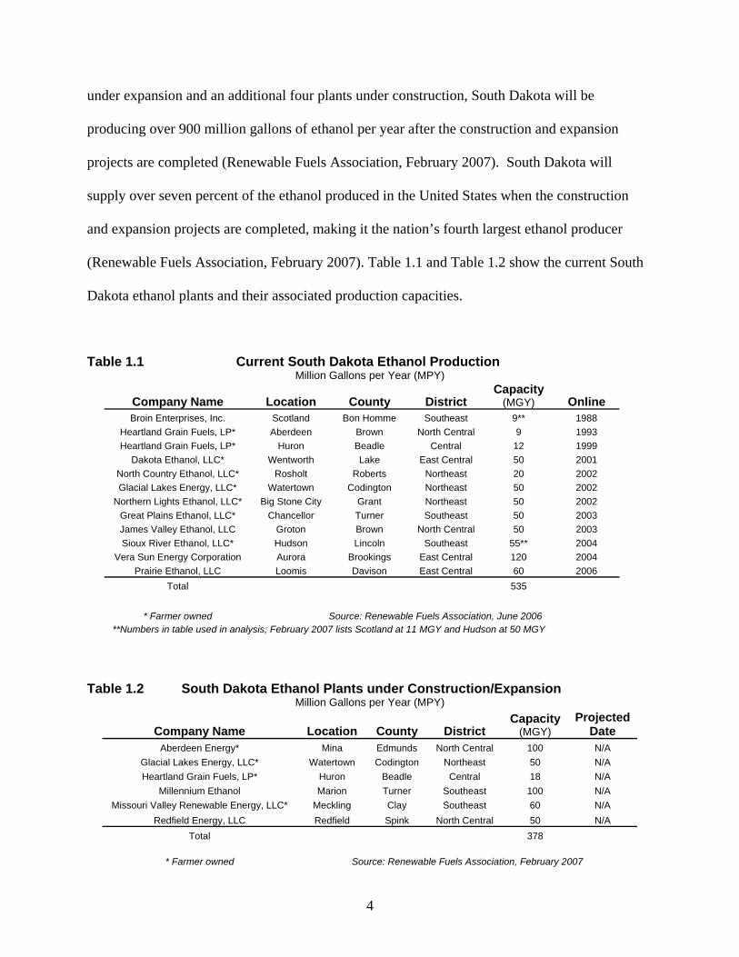
under expansion and an additional four plants under construction, South Dakota will be

producing over 900 million gallons of ethanol per year after the construction and expansion

projects are completed (Renewable Fuels Association, February 2007). South Dakota will

supply over seven percent of the ethanol produced in the United States when the construction

and expansion projects are completed, making it the nation’s fourth largest ethanol producer

(Renewable Fuels Association, February 2007). Table 1.1 and Table 1.2 show the current South

Dakota ethanol plants and their associated production capacities.

Table 1.1 Current South Dakota Ethanol Production Million Gallons per Year (MPY)

Company Name Location County District Capacity

(MGY) Online Broin Enterprises, Inc. Scotland Bon Homme Southeast 9** 1988

Heartland Grain Fuels, LP* Aberdeen Brown North Central 9 1993 Heartland Grain Fuels, LP* Huron Beadle Central 12 1999

Dakota Ethanol, LLC* Wentworth Lake East Central 50 2001 North Country Ethanol, LLC* Rosholt Roberts Northeast 20 2002 Glacial Lakes Energy, LLC* Watertown Codington Northeast 50 2002

Northern Lights Ethanol, LLC* Big Stone City Grant Northeast 50 2002 Great Plains Ethanol, LLC* Chancellor Turner Southeast 50 2003 James Valley Ethanol, LLC Groton Brown North Central 50 2003 Sioux River Ethanol, LLC* Hudson Lincoln Southeast 55** 2004

Vera Sun Energy Corporation Aurora Brookings East Central 120 2004 Prairie Ethanol, LLC Loomis Davison East Central 60 2006

Total 535

* Farmer owned Source: Renewable Fuels Association, June 2006 **Numbers in table used in analysis; February 2007 lists Scotland at 11 MGY and Hudson at 50 MGY

Table 1.2 South Dakota Ethanol Plants under Construction/Expansion

Million Gallons per Year (MPY)

Company Name Location County District Capacity

(MGY) Projected

Date Aberdeen Energy* Mina Edmunds North Central 100 N/A

Glacial Lakes Energy, LLC* Watertown Codington Northeast 50 N/A Heartland Grain Fuels, LP* Huron Beadle Central 18 N/A

Millennium Ethanol Marion Turner Southeast 100 N/A Missouri Valley Renewable Energy, LLC* Meckling Clay Southeast 60 N/A

Redfield Energy, LLC Redfield Spink North Central 50 N/A Total 378

* Farmer owned Source: Renewable Fuels Association, February 2007

5

Theory and Methods of Analysis

Basis is the difference between the local cash price and the futures price of a commodity.

Local corn basis in South Dakota has been affected by the production of ethanol within the state.

As the nation’s fourth largest ethanol producer, it is important to analyze the impacts that

increased ethanol production has on the South Dakota corn basis.

Formally, a basis ( tB ) is defined as a futures price ( tF ) minus a cash price ( tP ): tB = tF -

tP . If the futures price is above the cash price, the basis is positive, while if the futures price is

below the cash price, the basis is negative. These definitions follow a convention in the academic

literature, whereas commercial practice defines basis as cash minus futures, and thus reverses the

sign (Tomek & Robinson, 2003). The cash minus futures definition is used within this study. The

futures price is the Chicago price for grain, which is determined by the Chicago Board of Trade

(CBOT) and is used for corn, soybeans, and sorghum futures prices (Lutgen & Wasser, 2005).

An ordinary least squares (OLS) regression model was used to estimate the impacts of

ethanol production on the South Dakota corn basis. It was also used to project future impacts that

increased ethanol production may have on the corn basis. The model was estimated using

monthly data from January 1997 through December 2005 for each major corn producing district

in South Dakota as well as the “State” as represented by the five east river districts. The major

corn producing districts evaluated were the Northeast, East Central, Southeast, North Central,

and Central districts since almost all corn produced in South Dakota comes from those districts.

In 2005, 97.28% of all corn produced in South Dakota came from the five east river districts

(USDA NASS). To determine a “State” impact on the corn basis, the model was run using the

sum of the five east river districts. Data used was provided by Alan May, Extension Grain and

6

Marketing Specialist at South Dakota State University Economics Department and by the USDA

NASS.

Factors that can have an impact on the corn basis include but are not limited to futures

price, local supply and demand, local storage availability, and transportation costs.

The OLS regression model was used to estimate the impacts of futures prices, corn

production from grain, corn usage by ethanol, corn usage by cattle, storage availability, Midwest

No. 2 Diesel retail sales prices, and unit train transportation on the South Dakota corn basis.

Corn production from grain represents local supply; corn usage by ethanol and corn usage by

cattle represent local demand, and the Midwest No. 2. Diesel retail sales prices and unit train

transportation represent transportation costs.

The following regression equation is the basis model used for this analysis:

Basis = α + 1β (Futures Price) + 2β (Corn Production for Grain) + 3β (Corn

Usage by Ethanol) + 4β (Corn Usage by Cattle) + 5β (Midwest No. 2

Diesel Retail Sales Prices) + 6β (Storage Availability) + 7β (Unit Train

Transportation) + iμ

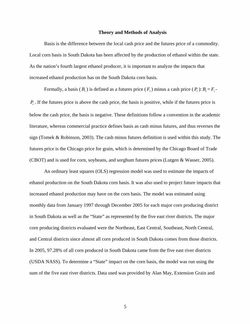
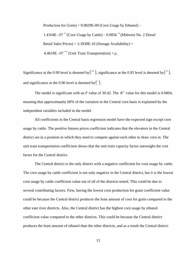
where futures price is in dollars per bushel, corn production for grain is in bushels, corn usage by

ethanol is in bushels, corn usage by cattle is in bushels, Midwest No. 2 Diesel retail sales prices

is in dollars per gallon, storage availability is in bushels, and unit train transportation is in dollars

per unit train car multiplied by the number of unit train cars.

7

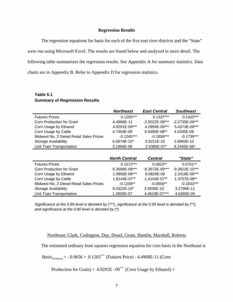
Regression Results

The regression equations for basis for each of the five east river districts and the “State”

were run using Microsoft Excel. The results are found below and analyzed in more detail. The

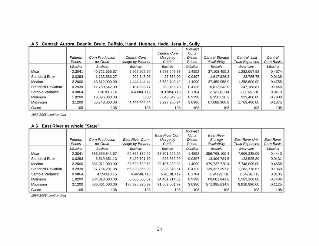
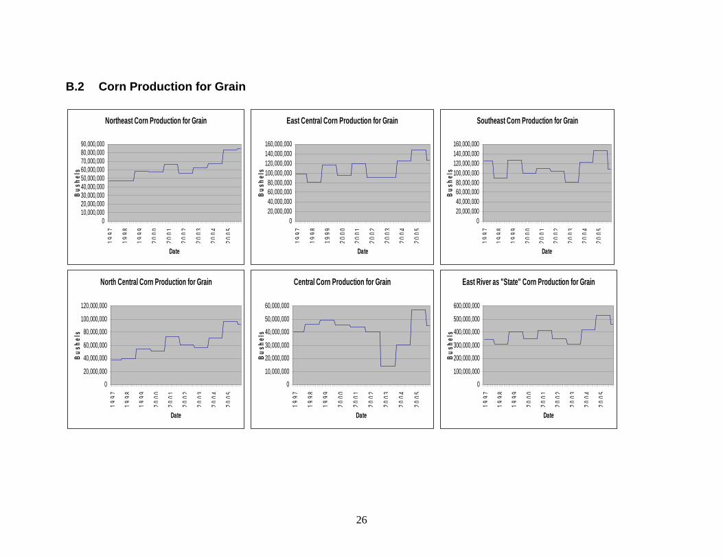
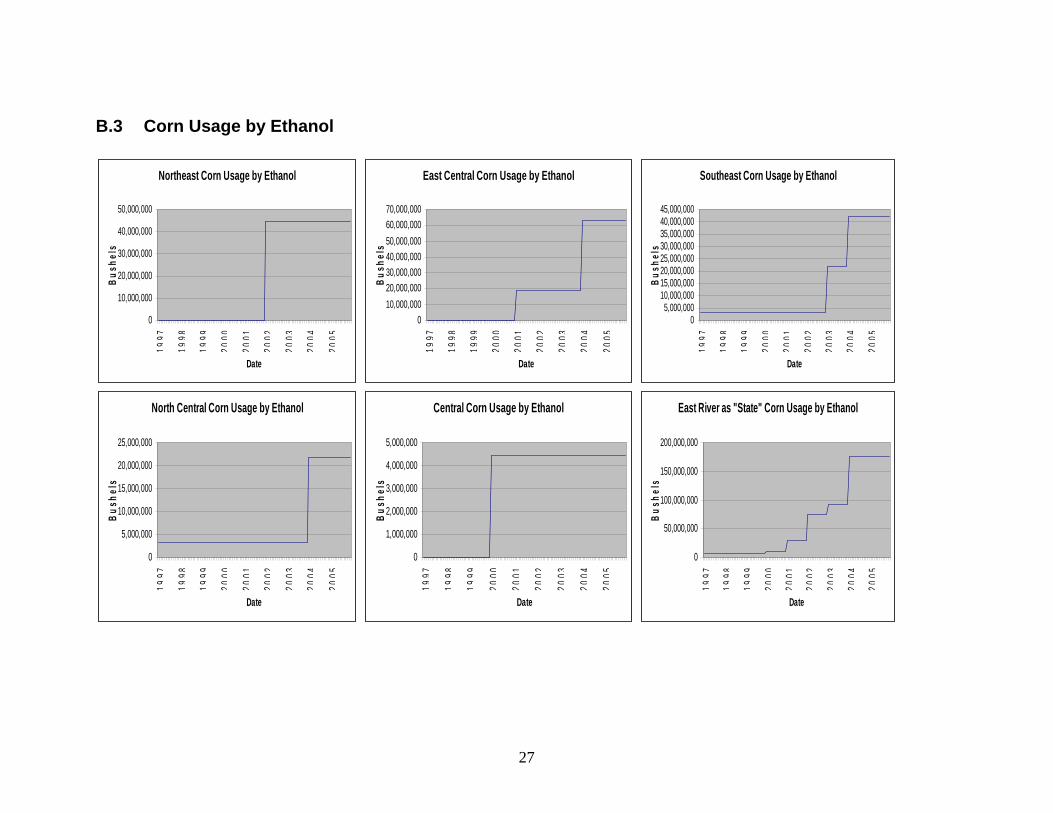
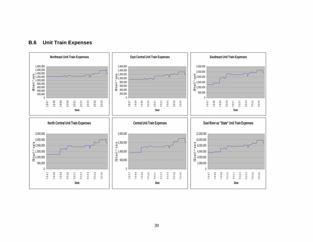
following table summarizes the regression results. See Appendix A for summary statistics. Data

charts are in Appendix B. Refer to Appendix D for regression statistics.

Table 5.1 Summary of Regression Results

Northeast East Central Southeast Futures Prices 0.1205*** 0.1337*** 0.1420***Corn Production for Grain -4.4968E-11 -2.5022E-09*** -2.2735E-09***Corn Usage by Ethanol 4.9291E-09*** 4.2993E-09*** 5.4373E-09***Corn Usage by Cattle 4.7454E-08 6.5480E-08** 4.0335E-08 Midwest No. 2 Diesel Retail Sales Prices -0.1245*** -0.1859*** -0.1739***Storage Availability 6.5874E-10* 3.6221E-10 2.6893E-10 Unit Train Transportation 3.1994E-08 2.9385E-07* 8.2445E-08*

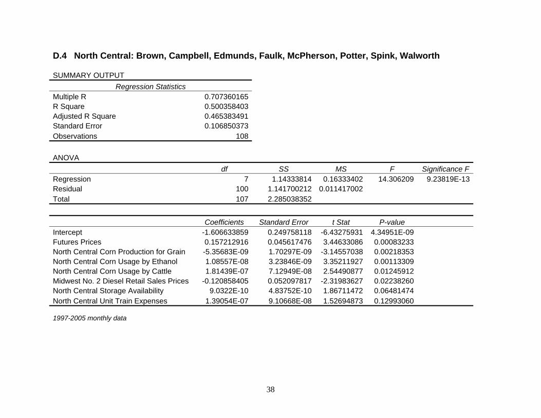
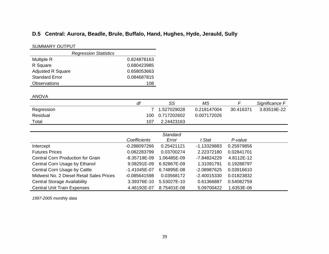
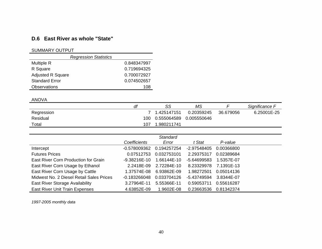
North Central Central "State" Futures Prices 0.1572*** 0.0823** 0.0751** Corn Production for Grain -5.3568E-09*** -8.3572E-09*** -9.3822E-10***Corn Usage by Ethanol 1.0856E-08*** 9.0829E-09 2.2418E-09***Corn Usage by Cattle 1.8144E-07** -1.4104E-07** 1.3757E-08** Midwest No. 2 Diesel Retail Sales Prices -0.1209** -0.0856** -0.1833***Storage Availability 9.0322E-10* 3.3938E-10 3.2796E-11 Unit Train Transportation 1.3905E-07 4.4619E-07*** 4.6385E-09 Significance at the 0.99 level is denoted by (***), significance at the 0.95 level is denoted by (**), and significance at the 0.90 level is denoted by (*).

Northeast: Clark, Codington, Day, Deuel, Grant, Hamlin, Marshall, Roberts

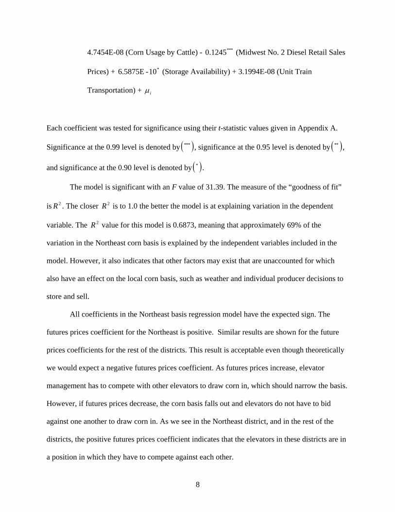
The estimated ordinary least squares regression equation for corn basis in the Northeast is

NortheastBasis = - 0.9656 + ***1205.0 (Futures Price) - 4.4968E-11 (Corn

Production for Grain) + ***09-4.9291E (Corn Usage by Ethanol) +

8

4.7454E-08 (Corn Usage by Cattle) - ***1245.0 (Midwest No. 2 Diesel Retail Sales

Prices) + *10-6.5875E (Storage Availability) + 3.1994E-08 (Unit Train

Transportation) + iμ

Each coefficient was tested for significance using their t-statistic values given in Appendix A.

Significance at the 0.99 level is denoted by ( )*** , significance at the 0.95 level is denoted by ( )** ,

and significance at the 0.90 level is denoted by ( )* .

The model is significant with an F value of 31.39. The measure of the “goodness of fit”

is 2R . The closer 2R is to 1.0 the better the model is at explaining variation in the dependent

variable. The 2R value for this model is 0.6873, meaning that approximately 69% of the

variation in the Northeast corn basis is explained by the independent variables included in the

model. However, it also indicates that other factors may exist that are unaccounted for which

also have an effect on the local corn basis, such as weather and individual producer decisions to

store and sell.

All coefficients in the Northeast basis regression model have the expected sign. The

futures prices coefficient for the Northeast is positive. Similar results are shown for the future

prices coefficients for the rest of the districts. This result is acceptable even though theoretically

we would expect a negative futures prices coefficient. As futures prices increase, elevator

management has to compete with other elevators to draw corn in, which should narrow the basis.

However, if futures prices decrease, the corn basis falls out and elevators do not have to bid

against one another to draw corn in. As we see in the Northeast district, and in the rest of the

districts, the positive futures prices coefficient indicates that the elevators in these districts are in

a position in which they have to compete against each other.

9

The unit train transportation coefficient for the Northeast is positive, but is statistically

insignificant. The expected sign on this coefficient is indeterminate. As explained earlier, unit

train transportation is determined by multiplying the number of cars on the unit train times the

expense rate per car depending on the size or number of cars on the unit train. Unit train car

capacity alone suggests a positive impact on corn basis, meaning basis would narrow, or become

positive as the number of unit train facilities within a district increase. As we see in the Northeast

district, and in the other districts, the capacity factor outweighs the cost factor for the unit trains

transportation coefficient, giving a positive coefficient value.

The Northeast district is the only district where the corn production coefficient is not

significant. The coefficient for corn usage by cattle is not significant in this district, where the

other districts, excluding the Southeast district, show significance. The storage availability

coefficient is significant for this district, where the other districts, excluding the North Central

district, show no significance. Also, unit train transportation is not significant in the Northeast

district.

East Central: Brookings, Davison, Hanson, Kingsbury, Lake,

McCook, Miner, Moody, Minnehaha, Sanborn

The estimated ordinary least squares regression equation for corn basis in the East

Central is

lEastCentraBasis = - 1.1113 + *** 0.1337 (Futures Price) - *** 09-2.5022E (Corn

Production for Grain) + *** 09-4.2993E (Corn Usage by Ethanol) +

** 08-6.5480E (Corn Usage by Cattle) - *** 0.1859 (Midwest No. 2 Diesel

Retail Sales Prices) + 10-3.6221E (Storage Availability) + * 07-2.9385E

(Unit Train Transportation) + iμ

10

Significance at the 0.99 level is denoted by ( )*** , significance at the 0.95 level is denoted by ( )** ,

and significance at the 0.90 level is denoted by ( )* .

The model is significant with an F value of 24.78. The 2R value for this model is 0.6344,

meaning that approximately 63% of the variation in the East Central corn basis is explained by

the independent variables included in the model.

All coefficients in the East Central basis regression model have the expected sign. As

explained earlier, the positive futures prices coefficient indicates that the elevators in the East

Central district are in a position in which they need to compete against each other to draw corn

in. The unit train transportation coefficient shows that the unit train capacity factor outweighs the

cost factor for the East Central district, giving a positive coefficient value.

The coefficients for the East Central are fairly consistent in significance with the other

districts, deviating with a 0.90 significance level for the unit train transportation coefficient

where other districts, excluding the Southeast and Central districts, show no significance.

Southeast: Bon Homme, Charles Mix, Clay, Douglas, Hutchinson,

Lincoln, Turner, Union, Yankton

The estimated ordinary least squares regression equation for corn basis in the Southeast is

SoutheastBasis = - 0.8225 + ***0.1420 (Futures Price) – *** 09-2.2735E (Corn

Production for Grain) + *** 09-5.4373E (Corn Usage by Ethanol) +

4.0335E-08 (Corn Usage by Cattle) - *** 0.1739 (Midwest No. 2 Diesel

Retail Sales Prices) + 2.6893E-10 (Storage Availability) +

* 08-8.2445E (Unit Train Transportation) + iμ

11

Significance at the 0.99 level is denoted by ( )*** , significance at the 0.95 level is denoted by ( )** ,

and significance at the 0.90 level is denoted by ( )* .

The model is significant with an F value of 21.01. The 2R value for this model is 0.5952,

meaning that approximately 60% of the variation in the Southeast corn basis is explained by the

independent variables included in the model.

All coefficients in the Southeast basis regression model have the expected sign. The

positive futures prices coefficient indicates that the elevators in the Southeast district are in a

position in which they need to compete against each other to draw corn in. The unit train

transportation coefficient shows that the unit train capacity factor outweighs the cost factor for

the Southeast district.

The coefficient for corn usage by cattle is not significant in this district; a similar result is

found for this coefficient in the Northeast district, while the other districts show significance.

The Southeast district also shows a 0.90 significance level for the unit train transportation

coefficient; a similar result is found for this coefficient in the East Central district, while the

other districts show no significance. All remaining coefficients for the Southeast are fairly

consistent in significance with the other districts tested.

North Central: Brown, Campbell, Edmunds, Faulk, McPherson,

Potter, Spink, Walworth

The estimated ordinary least squares regression equation for corn basis in the North

Central is

alNorthCentrBasis = - 1.6066 + *** 0.1572 (Futures Price) – *** 09-5.3568E (Corn

12

Production for Grain) + *** 08-1.0856E (Corn Usage by Ethanol) +

**07-1.8144E (Corn Usage by Cattle) - ** 0.1209 (Midwest No. 2 Diesel

Retail Sales Prices) + * 10-9.0322E (Storage Availability) +

07-1.3905E (Unit Train Transportation) + iμ

Significance at the 0.99 level is denoted by ( )*** , significance at the 0.95 level is denoted by ( )** ,

and significance at the 0.90 level is denoted by ( )* .

The model is significant with an F value of 14.31. The 2R value for this model is 0.5004,

meaning that approximately 50% of the variation in the North Central corn basis is explained by

the independent variables included in the model.

All coefficients in the North Central basis regression model have the expected sign. The

positive futures prices coefficient indicates that the elevators in the North Central district are in a

position in which they need to compete against each other to draw corn in. The unit train

transportation coefficient shows that the unit train capacity factor outweighs the cost factor for

the North Central district.

The coefficients for the North Central are fairly consistent in significance with the other

districts, deviating with a 0.90 significance level for the storage availability coefficient; a similar

result is found for this coefficient in the Northeast district, while the other districts show no

significance.

Central: Aurora, Beadle, Brule, Buffalo, Hand, Hughes, Hyde, Jerauld, Sully

The estimated ordinary least squares regression equation for corn basis in the Central is

CentralBasis = - 0.2881 + ** 0.0823 (Futures Price) – *** 09-8.3572E (Corn

13

Production for Grain) + 9.0829E-09 (Corn Usage by Ethanol) –

** 07-1.4104E (Corn Usage by Cattle) - ** 0.0856 (Midwest No. 2 Diesel

Retail Sales Prices) + 3.3938E-10 (Storage Availability) +

*** 07-4.4619E (Unit Train Transportation) + iμ

Significance at the 0.99 level is denoted by ( )*** , significance at the 0.95 level is denoted by ( )** ,

and significance at the 0.90 level is denoted by ( )* .

The model is significant with an F value of 30.42. The 2R value for this model is 0.6804,

meaning that approximately 68% of the variation in the Central corn basis is explained by the

independent variables included in the model.

All coefficients in the Central basis regression model have the expected sign except corn

usage by cattle. The positive futures prices coefficient indicates that the elevators in the Central

district are in a position in which they need to compete against each other to draw corn in. The

unit train transportation coefficient shows that the unit train capacity factor outweighs the cost

factor for the Central district.

The Central district is the only district with a negative coefficient for corn usage by cattle.

The corn usage by cattle coefficient is not only negative in the Central district, but it is the lowest

corn usage by cattle coefficient value out of all of the districts tested. This could be due to

several contributing factors. First, having the lowest corn production for grain coefficient value

could be because the Central district produces the least amount of corn for grain compared to the

other east river districts. Also, the Central district has the highest corn usage by ethanol

coefficient value compared to the other districts. This could be because the Central district

produces the least amount of ethanol than the other districts, and as a result the Central district

14

has the largest ratio of corn usage by ethanol to corn production for grain than the other districts.

It is also important to note that the Central district has the largest amount of cattle in the state,

but has the lowest number of cattle on feed (COF) of the five east river districts. The negative

coefficient value for corn usage by cattle for the Central district could be picking up on that

difference. All of these factors combined could potentially mean that the small number of COF is

less intensive in this district compared to the other districts, and that such a small market for

COF could explain the unexpected sign for the corn usage by cattle coefficient.

The Central district is the only district whose futures prices coefficient is not significant

at the 0.99 level. It is also the only district whose corn usage by ethanol coefficient is not

significant. This may be due to the fact that the Central district produces the least amount of corn

out of all the districts and has only one ethanol plant. The central district is also the only district

with a 0.99 significance level for the unit train transportation coefficient while the other districts

have lower significance levels or show no significance.

East River as “State”

The estimated ordinary least squares regression equation for corn basis in the “State” is

""StateBasis = - 0.5780 + ** 0.0751 (Futures Price) – *** 10-9.3822E (Corn

Production for Grain) + *** 09-2.2418E (Corn Usage by Ethanol) +

** 08-1.3757E (Corn Usage by Cattle) - *** 0.1833 (Midwest No. 2 Diesel

Retail Sales Prices) + 3.2796E-11 (Storage Availability) + 4.6385E-09 (Unit

Train Transportation) + iμ

15

Significance at the 0.99 level is denoted by ( )*** , significance at the 0.95 level is denoted by ( )** ,

and significance at the 0.90 level is denoted by ( )* .

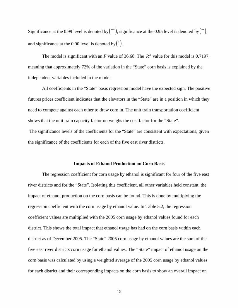
The model is significant with an F value of 36.68. The 2R value for this model is 0.7197,

meaning that approximately 72% of the variation in the “State” corn basis is explained by the

independent variables included in the model.

All coefficients in the “State” basis regression model have the expected sign. The positive

futures prices coefficient indicates that the elevators in the “State” are in a position in which they

need to compete against each other to draw corn in. The unit train transportation coefficient

shows that the unit train capacity factor outweighs the cost factor for the “State”.

The significance levels of the coefficients for the “State” are consistent with expectations, given

the significance of the coefficients for each of the five east river districts.

Impacts of Ethanol Production on Corn Basis

The regression coefficient for corn usage by ethanol is significant for four of the five east

river districts and for the “State”. Isolating this coefficient, all other variables held constant, the

impact of ethanol production on the corn basis can be found. This is done by multiplying the

regression coefficient with the corn usage by ethanol value. In Table 5.2, the regression

coefficient values are multiplied with the 2005 corn usage by ethanol values found for each

district. This shows the total impact that ethanol usage has had on the corn basis within each

district as of December 2005. The “State” 2005 corn usage by ethanol values are the sum of the

five east river districts corn usage for ethanol values. The “State” impact of ethanol usage on the

corn basis was calculated by using a weighted average of the 2005 corn usage by ethanol values

for each district and their corresponding impacts on the corn basis to show an overall impact on

16

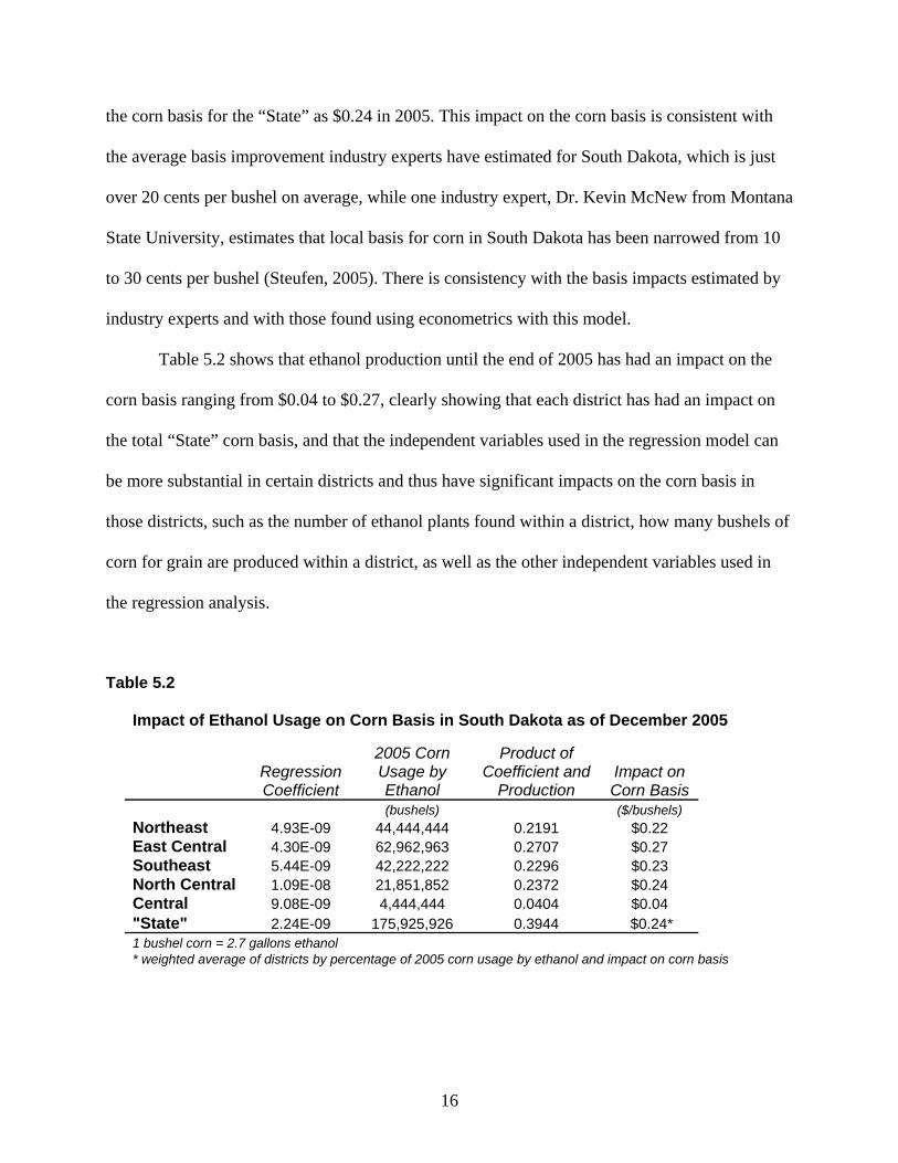
the corn basis for the “State” as $0.24 in 2005. This impact on the corn basis is consistent with

the average basis improvement industry experts have estimated for South Dakota, which is just

over 20 cents per bushel on average, while one industry expert, Dr. Kevin McNew from Montana

State University, estimates that local basis for corn in South Dakota has been narrowed from 10

to 30 cents per bushel (Steufen, 2005). There is consistency with the basis impacts estimated by

industry experts and with those found using econometrics with this model.

Table 5.2 shows that ethanol production until the end of 2005 has had an impact on the

corn basis ranging from $0.04 to $0.27, clearly showing that each district has had an impact on

the total “State” corn basis, and that the independent variables used in the regression model can

be more substantial in certain districts and thus have significant impacts on the corn basis in

those districts, such as the number of ethanol plants found within a district, how many bushels of

corn for grain are produced within a district, as well as the other independent variables used in

the regression analysis.

Table 5.2

Impact of Ethanol Usage on Corn Basis in South Dakota as of December 2005

Regression Coefficient

2005 Corn Usage by Ethanol

Product of Coefficient and

Production Impact on Corn Basis

(bushels) ($/bushels) Northeast 4.93E-09 44,444,444 0.2191 $0.22 East Central 4.30E-09 62,962,963 0.2707 $0.27 Southeast 5.44E-09 42,222,222 0.2296 $0.23 North Central 1.09E-08 21,851,852 0.2372 $0.24 Central 9.08E-09 4,444,444 0.0404 $0.04 "State" 2.24E-09 175,925,926 0.3944 $0.24* 1 bushel corn = 2.7 gallons ethanol * weighted average of districts by percentage of 2005 corn usage by ethanol and impact on corn basis

17

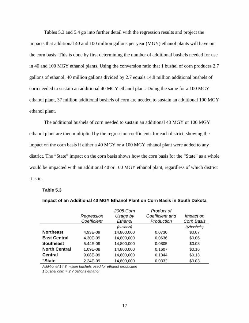
Tables 5.3 and 5.4 go into further detail with the regression results and project the

impacts that additional 40 and 100 million gallons per year (MGY) ethanol plants will have on

the corn basis. This is done by first determining the number of additional bushels needed for use

in 40 and 100 MGY ethanol plants. Using the conversion ratio that 1 bushel of corn produces 2.7

gallons of ethanol, 40 million gallons divided by 2.7 equals 14.8 million additional bushels of

corn needed to sustain an additional 40 MGY ethanol plant. Doing the same for a 100 MGY

ethanol plant, 37 million additional bushels of corn are needed to sustain an additional 100 MGY

ethanol plant.

The additional bushels of corn needed to sustain an additional 40 MGY or 100 MGY

ethanol plant are then multiplied by the regression coefficients for each district, showing the

impact on the corn basis if either a 40 MGY or a 100 MGY ethanol plant were added to any

district. The “State” impact on the corn basis shows how the corn basis for the “State” as a whole

would be impacted with an additional 40 or 100 MGY ethanol plant, regardless of which district

it is in.

Table 5.3 Impact of an Additional 40 MGY Ethanol Plant on Corn Basis in South Dakota

Regression Coefficient

2005 Corn Usage by Ethanol

Product of Coefficient and

Production Impact on Corn Basis

(bushels) ($/bushels) Northeast 4.93E-09 14,800,000 0.0730 $0.07 East Central 4.30E-09 14,800,000 0.0636 $0.06 Southeast 5.44E-09 14,800,000 0.0805 $0.08 North Central 1.09E-08 14,800,000 0.1607 $0.16 Central 9.08E-09 14,800,000 0.1344 $0.13 "State" 2.24E-09 14,800,000 0.0332 $0.03 Additional 14.8 million bushels used for ethanol production 1 bushel corn = 2.7 gallons ethanol

18

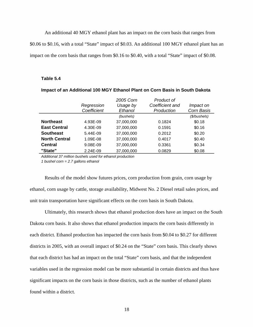
An additional 40 MGY ethanol plant has an impact on the corn basis that ranges from

$0.06 to $0.16, with a total “State” impact of $0.03. An additional 100 MGY ethanol plant has an

impact on the corn basis that ranges from $0.16 to $0.40, with a total “State” impact of $0.08.

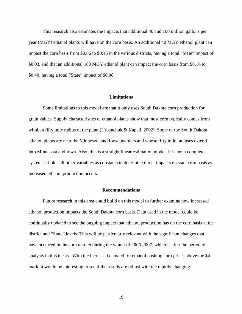
Table 5.4 Impact of an Additional 100 MGY Ethanol Plant on Corn Basis in South Dakota

Regression Coefficient

2005 Corn Usage by Ethanol

Product of Coefficient and

Production Impact on Corn Basis

(bushels) ($/bushels) Northeast 4.93E-09 37,000,000 0.1824 $0.18 East Central 4.30E-09 37,000,000 0.1591 $0.16 Southeast 5.44E-09 37,000,000 0.2012 $0.20 North Central 1.09E-08 37,000,000 0.4017 $0.40 Central 9.08E-09 37,000,000 0.3361 $0.34 "State" 2.24E-09 37,000,000 0.0829 $0.08 Additional 37 million bushels used for ethanol production 1 bushel corn = 2.7 gallons ethanol

Results of the model show futures prices, corn production from grain, corn usage by

ethanol, corn usage by cattle, storage availability, Midwest No. 2 Diesel retail sales prices, and

unit train transportation have significant effects on the corn basis in South Dakota.

Ultimately, this research shows that ethanol production does have an impact on the South

Dakota corn basis. It also shows that ethanol production impacts the corn basis differently in

each district. Ethanol production has impacted the corn basis from $0.04 to $0.27 for different

districts in 2005, with an overall impact of $0.24 on the “State” corn basis. This clearly shows

that each district has had an impact on the total “State” corn basis, and that the independent

variables used in the regression model can be more substantial in certain districts and thus have

significant impacts on the corn basis in those districts, such as the number of ethanol plants

found within a district.

19

This research also estimates the impacts that additional 40 and 100 million gallons per

year (MGY) ethanol plants will have on the corn basis. An additional 40 MGY ethanol plant can

impact the corn basis from $0.06 to $0.16 in the various districts, having a total “State” impact of

$0.03, and that an additional 100 MGY ethanol plant can impact the corn basis from $0.16 to

$0.40, having a total “State” impact of $0.08.

Limitations

Some limitations to this model are that it only uses South Dakota corn production for

grain values. Supply characteristics of ethanol plants show that most corn typically comes from

within a fifty mile radius of the plant (Urbanchuk & Kapell, 2002). Some of the South Dakota

ethanol plants are near the Minnesota and Iowa boarders and whose fifty mile radiuses extend

into Minnesota and Iowa. Also, this is a straight linear estimation model. It is not a complete

system. It holds all other variables as constants to determine direct impacts on state corn basis as

increased ethanol production occurs.

Recommendations

Future research in this area could build on this model to further examine how increased

ethanol production impacts the South Dakota corn basis. Data used in the model could be

continually updated to see the ongoing impact that ethanol production has on the corn basis at the

district and “State” levels. This will be particularly relevant with the significant changes that

have occurred in the corn market during the winter of 2006-2007, which is after the period of

analysis in this thesis. With the increased demand for ethanol pushing corn prices above the $4

mark, it would be interesting to see if the results are robust with the rapidly changing

20

corn/ethanol markets. Further research could also try to determine how county level corn basis is

impacted.

The model could also be used to see the impacts that any new mandates for increased

ethanol production would have on the district and “State” corn basis, and to see if any future

mandates for increased ethanol production actually increase the price of corn. Such future

mandates could be similar to President George W. Bush’s Advanced Energy Initiative, in which

a national goal is set to replace more than 75% of U.S. oil imports from the Middle East by 2025.

It might also be interesting to apply this model to other states to determine how their corn

basis has been impacted by ethanol production and make comparisons. The model could possibly

be extended to include multiple states to determine how regional corn basis has been impacted

by ethanol production.

Future research could also determine if this model could be applied to the bio-diesel

industry to determine the impacts of increased bio-diesel production on the soybean basis.

References

BNSF Railway, Grain Elevator Directory, List of Facilities in South Dakota, http://www.bnsf.com/markets/agricultural/elevator/menu/sdlist.html Farm Net Services, Information for the Ag Industry, South Dakota Grain Elevators, http://www.farmnetservices.com/farm/Grain_Elevators/South_Dakota/69-0.html Lutgen, Lynn, and Diane Wasser, “Basis Patterns for Selected Sites in Nebraska for Corn, Wheat, Sorghum, and Soybeans,” October 2005. http://agrecon.unl.edu/Basis/Basis.htm. Renewable Fuels Association, http://www.ethanolrfa.org South Dakota Department of Transportation Office of Railroads, http://www.sddot.com/fpa/railroad/ Stuefen, Randall M., The Economic Impact of Ethanol Plants in South Dakota, Stuefen Research, LLC, December 27, 2005.

21

Tomek, William G. with Kenneth L. Robinson, “Agricultural Product Prices,” Fourth Edition, Cornell University Press, 2003. United States Department of Agriculture, Agricultural Marketing Service, “Grain Transportation Report”, http://www.ams.usda.gov/tmdtsb/grain/ United States Department of Agriculture, National Agriculture Statistics Service, http://www.nass.usda.gov United States Energy Information Administration, “Midwest No. 2 Diesel Retail Sales by All Sellers (Cents per Gallon),” http://tonto.eia.doe.gov/dnav/pet/hist/ddr003M.htm Urbanchuk, John M., and Jeff Kapell, “Ethanol and the Local Community,” June 20, 2002. http://www.ncga.com/ethanol/pdfs/EthanolLocalCommunity.pdf Urbanchuk, John M., “Contribution of the Ethanol Industry to the Economy of the United States,” LECG, February 19, 2007. http://www.ethanolrfa.org/objects/documents//2006_ethanol_economic_contribution.pdf

22

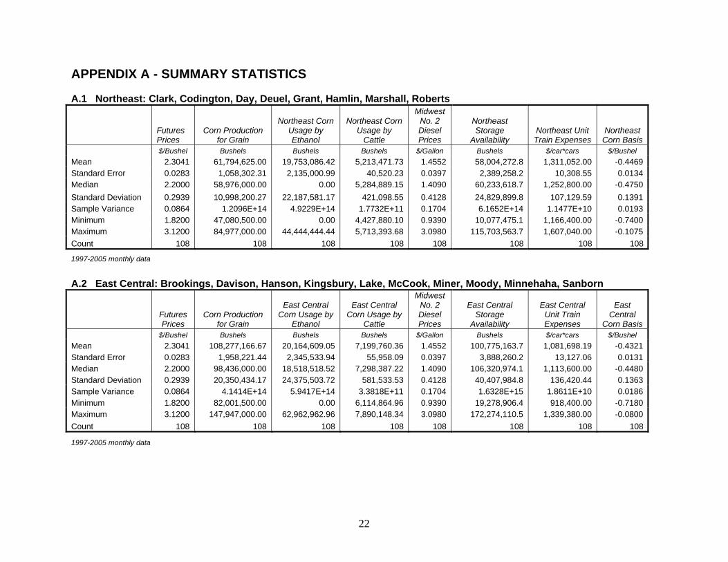
APPENDIX A - SUMMARY STATISTICS A.1 Northeast: Clark, Codington, Day, Deuel, Grant, Hamlin, Marshall, Roberts

Futures Prices

Corn Production for Grain

Northeast Corn Usage by Ethanol

Northeast Corn Usage by

Cattle

Midwest No. 2 Diesel Prices

Northeast Storage

Availability Northeast Unit

Train Expenses Northeast Corn Basis

$/Bushel Bushels Bushels Bushels $/Gallon Bushels $/car*cars $/Bushel Mean 2.3041 61,794,625.00 19,753,086.42 5,213,471.73 1.4552 58,004,272.8 1,311,052.00 -0.4469Standard Error 0.0283 1,058,302.31 2,135,000.99 40,520.23 0.0397 2,389,258.2 10,308.55 0.0134Median 2.2000 58,976,000.00 0.00 5,284,889.15 1.4090 60,233,618.7 1,252,800.00 -0.4750Standard Deviation 0.2939 10,998,200.27 22,187,581.17 421,098.55 0.4128 24,829,899.8 107,129.59 0.1391Sample Variance 0.0864 1.2096E+14 4.9229E+14 1.7732E+11 0.1704 6.1652E+14 1.1477E+10 0.0193Minimum 1.8200 47,080,500.00 0.00 4,427,880.10 0.9390 10,077,475.1 1,166,400.00 -0.7400Maximum 3.1200 84,977,000.00 44,444,444.44 5,713,393.68 3.0980 115,703,563.7 1,607,040.00 -0.1075Count 108 108 108 108 108 108 108 108

1997-2005 monthly data A.2 East Central: Brookings, Davison, Hanson, Kingsbury, Lake, McCook, Miner, Moody, Minnehaha, Sanborn

Futures Prices

Corn Production for Grain

East Central Corn Usage by

Ethanol

East Central Corn Usage by

Cattle

Midwest No. 2 Diesel Prices

East Central Storage

Availability

East Central Unit Train Expenses

East Central

Corn Basis $/Bushel Bushels Bushels Bushels $/Gallon Bushels $/car*cars $/Bushel

Mean 2.3041 108,277,166.67 20,164,609.05 7,199,760.36 1.4552 100,775,163.7 1,081,698.19 -0.4321Standard Error 0.0283 1,958,221.44 2,345,533.94 55,958.09 0.0397 3,888,260.2 13,127.06 0.0131Median 2.2000 98,436,000.00 18,518,518.52 7,298,387.22 1.4090 106,320,974.1 1,113,600.00 -0.4480Standard Deviation 0.2939 20,350,434.17 24,375,503.72 581,533.53 0.4128 40,407,984.8 136,420.44 0.1363Sample Variance 0.0864 4.1414E+14 5.9417E+14 3.3818E+11 0.1704 1.6328E+15 1.8611E+10 0.0186Minimum 1.8200 82,001,500.00 0.00 6,114,864.96 0.9390 19,278,906.4 918,400.00 -0.7180Maximum 3.1200 147,947,000.00 62,962,962.96 7,890,148.34 3.0980 172,274,110.5 1,339,380.00 -0.0800Count 108 108 108 108 108 108 108 108

1997-2005 monthly data

23

A.3 Southeast: Bon Homme, Charles Mix, Clay, Douglas, Hutchinson, Lincoln, Turner, Union, Yankton

Futures Prices

Corn Production for Grain

Southeast Corn Usage by Ethanol

Southeast Corn Usage by

Cattle

Midwest No. 2 Diesel Prices

Southeast Storage

Availability Southeast Unit Train Expenses

Southeast Corn Basis

$/Bushel Bushels Bushels Bushels $/Gallon Bushels $/car*cars $/Bushel Mean 2.3041 111,376,791.67 14,032,921.81 7,946,787.82 1.4552 104,222,635.2 2,078,750.69 -0.4054Standard Error 0.0283 1,869,048.73 1,557,914.89 61,764.15 0.0397 3,994,864.1 43,260.51 0.0117Median 2.2000 109,670,000.00 3,333,333.33 8,055,647.92 1.4090 110,221,883.5 2,227,200.00 -0.4210Standard Deviation 0.2939 19,423,724.21 16,190,326.44 641,871.86 0.4128 41,515,845.6 449,576.45 0.1213Sample Variance 0.0864 3.7728E+14 2.6213E+14 4.1200E+11 0.1704 1.7236E+15 2.0212E+11 0.0147Minimum 1.8200 81,568,000.00 3,333,333.33 6,749,326.64 0.9390 17,303,454.9 1,242,600.00 -0.6920Maximum 3.1200 147,217,000.00 42,222,222.22 8,708,808.57 3.0980 167,890,077.9 2,678,760.00 -0.1300Count 108 108 108 108 108 108 108 108

1997-2005 monthly data

A.4 North Central: Brown, Campbell, Edmunds, Faulk, McPherson, Potter, Spink, Walworth

Futures Prices

Corn Production for Grain

North Central Corn Usage by

Ethanol

North Central Corn Usage by

Cattle

Midwest No. 2 Diesel Prices

North Central Storage

Availability

North Central Unit Train Expenses

North Central

Corn Basis $/Bushel Bushels Bushels Bushels $/Gallon Bushels $/car*cars $/Bushel

Mean 2.3041 61,485,591.67 7,448,559.67 4,858,026.31 1.4552 56,657,573.6 1,852,766.24 -0.4785Standard Error 0.0283 1,682,017.13 744,279.16 37,757.63 0.0397 2,427,701.8 37,967.93 0.0141Median 2.2000 56,019,000.00 3,333,333.33 4,924,574.62 1.4090 53,684,962.6 1,896,600.00 -0.5068Standard Deviation 0.2939 17,480,034.80 7,734,775.94 392,388.78 0.4128 25,229,417.4 394,574.33 0.1461Sample Variance 0.0864 3.0555E+14 5.9827E+13 1.5397E+11 0.1704 6.3652E+14 1.5569E+11 0.0214Minimum 1.8200 36,908,100.00 3,333,333.33 4,125,994.95 0.9390 9,242,071.3 1,231,200.00 -0.7780Maximum 3.1200 95,617,000.00 21,851,851.85 5,323,864.45 3.0980 103,305,567.8 2,522,400.00 -0.1075Count 108 108 108 108 108 108 108 1081997-2005 monthly data

24

A.5 Central: Aurora, Beadle, Brule, Buffalo, Hand, Hughes, Hyde, Jerauld, Sully

Futures Prices

Corn Production for Grain

Central Corn Usage by Ethanol

Central Corn Usage by

Cattle

Midwest No. 2 Diesel Prices

Central Storage Availability

Central Unit Train Expenses

Central Corn Basis

$/Bushel Bushels Bushels Bushels $/Gallon Bushels $/car*cars $/Bushel Mean 2.3041 40,721,666.67 2,962,962.96 3,583,649.33 1.4552 37,108,455.2 1,282,067.98 -0.4574Standard Error 0.0283 1,133,583.27 202,543.98 27,852.90 0.0397 1,617,826.2 23,785.75 0.0139Median 2.2000 43,812,000.00 4,444,444.44 3,632,740.42 1.4090 37,459,058.9 1,258,600.00 -0.4755Standard Deviation 0.2939 11,780,542.90 2,104,898.77 289,455.78 0.4128 16,812,943.0 247,188.81 0.1448Sample Variance 0.0864 1.3878E+14 4.4306E+12 8.3785E+10 0.1704 2.8268E+14 6.1102E+10 0.0210Minimum 1.8200 13,696,000.00 0.00 3,043,647.38 0.9390 6,350,530.2 923,400.00 -0.7900Maximum 3.1200 56,748,000.00 4,444,444.44 3,927,286.94 3.0980 67,688,300.8 1,763,400.00 -0.1375Count 108 108 108 108 108 108 108 108

1997-2005 monthly data A.6 East River as whole "State"

Futures Prices

Corn Production for Grain

East River Corn Usage by Ethanol

East River Corn Usage by

Cattle

Midwest No. 2 Diesel Prices

East River Storage

Availability East River Unit Train Expenses

East River Corn Basis

$/Bushel Bushels Bushels Bushels $/Gallon Bushels $/car*cars $/Bushel Mean 2.3041 383,655,841.67 64,362,139.92 28,801,695.55 1.4552 356,768,100.4 7,606,335.09 -0.4440Standard Error 0.0283 6,519,651.13 6,429,791.70 223,852.99 0.0397 13,406,784.5 123,525.89 0.0131Median 2.2000 351,071,000.00 29,629,629.63 29,196,239.32 1.4090 379,737,720.4 7,748,800.00 -0.4658Standard Deviation 0.2939 67,754,201.98 66,820,355.39 2,326,348.51 0.4128 139,327,391.8 1,283,718.67 0.1360Sample Variance 0.0864 4.5906E+15 4.4650E+15 5.4119E+12 0.1704 1.9412E+16 1.6479E+12 0.0185Minimum 1.8200 304,813,000.00 6,666,666.67 24,461,714.03 0.9390 69,001,841.8 5,563,200.00 -0.7436Maximum 3.1200 530,661,000.00 175,925,925.93 31,563,501.97 3.0980 571,995,614.5 9,910,980.00 -0.1125Count 108 108 108 108 108 108 108 1081997-2005 monthly data

25

APPENDIX B - DATA CHARTS B.1 BASIS

Northeast Basis

-0.8

-0.7

-0.6

-0.5

-0.4

-0.3

-0.2

-0.1

0.0

1997

1998

1999

2000

2001

2002

2003

2004

2005

Date

Bas

is

East Central Basis

-0.8

-0.7

-0.6

-0.5

-0.4

-0.3

-0.2

-0.1

0.0

1997

1998

1999

2000

2001

2002

2003

2004

2005

Date

Bas

is

Southeast Basis

-0.8

-0.7

-0.6

-0.5

-0.4

-0.3

-0.2

-0.1

0.0

1997

1998

1999

200 0

2001

2002

2003

2004

2005

Date

Bas

is

North Central Basis

-0.9

-0.8

-0.7

-0.6

-0.5

-0.4

-0.3

-0.2

-0.1

0.0

1997

1998

1999

2000

2001

2002

2003

2004

2005

Date

Bas

is

Central Basis

-0.9

-0.8

-0.7

-0.6

-0.5

-0.4

-0.3

-0.2

-0.1

0.0

1997

1998

1999

2 000

2001

2002

2003

2004

2005

Date

Bas

is

East River as whole "State" Basis

-0.8

-0.7

-0.6

-0.5

-0.4

-0.3

-0.2

-0.1

0.0

1997

1998

199 9

2000

2001

2002

2003

2004

2005

DateB

asis

26

B.2 Corn Production for Grain

Northeast Corn Production for Grain

010,000,00020,000,00030,000,00040,000,00050,000,00060,000,00070,000,00080,000,00090,000,000

1997

1 998

1999

2000

2001

2002

2003

2004

2 005

Date

Bus

hels

East Central Corn Production for Grain

020,000,00040,000,00060,000,00080,000,000

100,000,000120,000,000140,000,000160,000,000

1997

1998

1999

2000

2001

2002

2003

2004

2005

DateB

ushe

ls

Southeast Corn Production for Grain

020,000,00040,000,00060,000,00080,000,000

100,000,000120,000,000140,000,000160,000,000

1997

1 998

199 9

200 0

2001

2002

2003

2 004

200 5

Date

Bus

hels

North Central Corn Production for Grain

0

20,000,000

40,000,000

60,000,000

80,000,000

100,000,000

120,000,000

199 7

199 8

1999

2000

2001

2002

2003

2 004

2 005

Date

Bush

els

Central Corn Production for Grain

0

10,000,000

20,000,000

30,000,000

40,000,000

50,000,000

60,000,00019

97

199 8

199 9

2 000

2 001

2 002

2003

2004

2005

Date

Bush

els

East River as "State" Corn Production for Grain

0

100,000,000

200,000,000

300,000,000

400,000,000

500,000,000

600,000,000

1997

199 8

1999

2000

2001

2002

2003

2 004

2 005

Date

Bush

els

27

B.3 Corn Usage by Ethanol

Northeast Corn Usage by Ethanol

0

10,000,000

20,000,000

30,000,000

40,000,000

50,000,000

1997

1 998

1999

2000

2001

2002

2003

200 4

2 005

Date

Bush

els

East Central Corn Usage by Ethanol

010,000,00020,000,00030,000,00040,000,00050,000,00060,000,00070,000,000

1997

199 8

1999

2 000

2 001

2002

2003

2004

2005

DateBu

shel

s

Southeast Corn Usage by Ethanol

05,000,000

10,000,00015,000,00020,000,00025,000,00030,000,00035,000,00040,000,00045,000,000

199 7

199 8

1999

2 000

2 001

2 002

2 003

2004

200 5

Date

Bush

els

North Central Corn Usage by Ethanol

0

5,000,000

10,000,000

15,000,000

20,000,000

25,000,000

1997

1 998

1 999

2000

2001

2002

2003

2004

2 005

Date

Bush

els

Central Corn Usage by Ethanol

0

1,000,000

2,000,000

3,000,000

4,000,000

5,000,00019

97

1998

1999

2000

200 1

2 00 2

2 003

2004

2005

Date

Bush

els

East River as "State" Corn Usage by Ethanol

0

50,000,000

100,000,000

150,000,000

200,000,000

1997

1 998

199 9

200 0

2001

2 002

2003

2 004

2005

Date

Bush

els

28

B.4 Corn Usage by Cattle

Northeast Corn Usage by Cattle

0

1,000,000

2,000,000

3,000,000

4,000,000

5,000,000

6,000,000

1997

1998

1999

2000

2001

200 2

2 003

2004

200 5

Date

Bush

els

East Central Corn Usage by Cattle

01,000,0002,000,0003,000,0004,000,0005,000,0006,000,0007,000,0008,000,0009,000,000

1997

1998

1999

2000

200 1

2 002

2 003

2004

2005

DateB

ushe

ls

Southeast Corn Usage by Cattle

0

2,000,000

4,000,000

6,000,000

8,000,000

10,000,000

1997

1 998

1999

2000

2001

2002

2003

200 4

2 005

Date

Bus

hels

North Central Corn Usage by Cattle

0

1,000,000

2,000,000

3,000,000

4,000,000

5,000,000

6,000,000

199 7

1998

1999

200 0

2001

2002

2 00 3

2004

2005

Date

Bus

hels

Central Corn Usage by Cattle

0500,000

1,000,0001,500,0002,000,0002,500,0003,000,0003,500,0004,000,0004,500,000

1997

1998

1999

2000

2001

2 00 2

2 003

2004

2005

Date

Bus

hels

East River as "State" Corn Usage by Cattle

05,000,000

10,000,00015,000,00020,000,00025,000,00030,000,00035,000,000

199 7

1 998

1 999

2000

2001

2002

2003

2004

2 00 5

Date

Bus

hels

29

B.5 Storage Availability

Northeast Storage Availability

020,000,00040,000,00060,000,00080,000,000

100,000,000120,000,000140,000,000

1997

1 998

1 999

2000

2001

2002

2003

200 4

200 5

Date

Bush

els

East Central Storage Availability

0

50,000,000

100,000,000

150,000,000

200,000,000

1997

1998

1 999

2000

2 001

200 2

2 003

200 4

2005

Date

Bush

els

Southeast Storage Availability

020,000,00040,000,00060,000,00080,000,000

100,000,000120,000,000140,000,000160,000,000180,000,000

1997

1 998

199 9

200 0

2001

2002

2003

2 004

200 5

Date

Bush

els

North Central Storage Availability

0

20,000,000

40,000,000

60,000,000

80,000,000

100,000,000

120,000,000

1997

1 99 8

1 999

2 000

2001

2002

2003

2004

200 5

Date

Bush

els

Central Storage Availability

010,000,00020,000,00030,000,00040,000,00050,000,00060,000,00070,000,00080,000,000

199 7

1 998

1999

2000

2001

2002

200 3

2 004

2005

Date

Bush

els

East River as "State" Storage Availability

0100,000,000200,000,000300,000,000400,000,000500,000,000600,000,000700,000,000

199 7

199 8

1999

2000

2001

2002

2003

2 004

2 005

Date

Bush

els

30

B.6 Unit Train Expenses

Northeast Unit Train Expenses

0200,000400,000600,000800,000

1,000,0001,200,0001,400,0001,600,0001,800,000

1997

1998

1999

2000

200 1

200 2

2003

2004

2005

Date

($/c

ar) *

car

s

East Central Unit Train Expenses

0200,000400,000600,000800,000

1,000,0001,200,0001,400,0001,600,000

1997

1998

1 999

200 0

2 001

200 2

2003

200 4

2005

Date

($/c

ar) *

car

s

Southeast Unit Train Expenses

0

500,000

1,000,000

1,500,000

2,000,000

2,500,000

3,000,000

1997

199 8

199 9

2 000

200 1

2 002

2003

2004

2005

Date

($/c

ar) *

car

s

North Central Unit Train Expenses

0

500,000

1,000,000

1,500,000

2,000,000

2,500,000

3,000,000

1997

1998

1999

2000

2001

2002

2003

2004

200 5

Date

($/c

ar) *

car

s

Central Unit Train Expenses

0

500,000

1,000,000

1,500,000

2,000,00019

97

199 8

1 99 9

2000

2 00 1

2002

2 003

2004

2 005

Date

($/c

ar) *

car

s

East River as "State" Unit Train Expenses

0

2,000,000

4,000,000

6,000,000

8,000,000

10,000,000

12,000,000

1997

1998

199 9

2 00 0

2 00 1

2 00 2

2 003

2004

2005

Date

($/c

ar) *

car

s

31

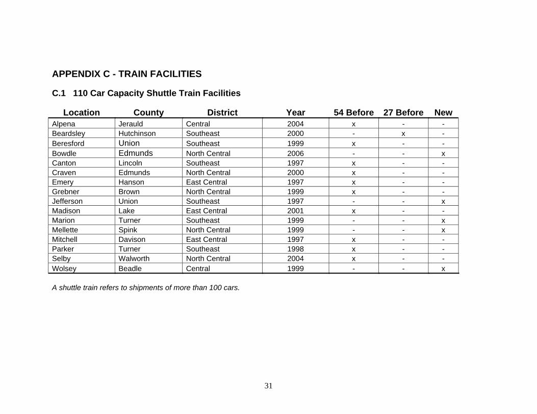
APPENDIX C - TRAIN FACILITIES C.1 110 Car Capacity Shuttle Train Facilities

Location County District Year 54 Before 27 Before New Alpena Jerauld Central 2004 x - - Beardsley Hutchinson Southeast 2000 - x - Beresford Union Southeast 1999 x - - Bowdle Edmunds North Central 2006 - - x Canton Lincoln Southeast 1997 x - - Craven Edmunds North Central 2000 x - - Emery Hanson East Central 1997 x - - Grebner Brown North Central 1999 x - - Jefferson Union Southeast 1997 - - x Madison Lake East Central 2001 x - - Marion Turner Southeast 1999 - - x Mellette Spink North Central 1999 - - x Mitchell Davison East Central 1997 x - - Parker Turner Southeast 1998 x - - Selby Walworth North Central 2004 x - - Wolsey Beadle Central 1999 - - x A shuttle train refers to shipments of more than 100 cars.

32

C.2 54 Car Capacity Unit Train Facilities

Location County District Year Aberdeen Brown North Central 1993 Bristol Day Northeast 87-88 Harrold Hughes Central * Huron Beadle Central 80's Mansfield Brown North Central * Milbank Grant Northeast * Northville Spink North Central * Onida Sully Central * Pierre Hughes Central * Redfield Spink North Central 96-97 Rosholt Roberts Northeast * Sioux Falls Minnehaha East Central * Sisseton Roberts Northeast * Vermillion Clay Southeast 1995 Vienna Clark Northeast 1994 Watertown Codington Northeast 1981 Watertown Codington Northeast 1993 Wentworth Lake East Central * Willow Lake Clark Northeast early 90's Yale Beadle Central 1996 Yankton Yankton Southeast early 80's * Assumed to have been in operation at 54 unit capacity before 1997 A unit train refers to shipments of a least 52 cars.

33

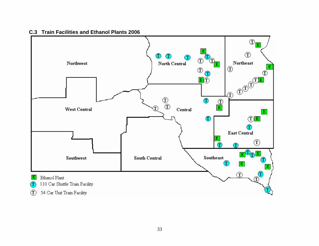
C.3 Train Facilities and Ethanol Plants 2006

34

C.4 State District and County Map

35

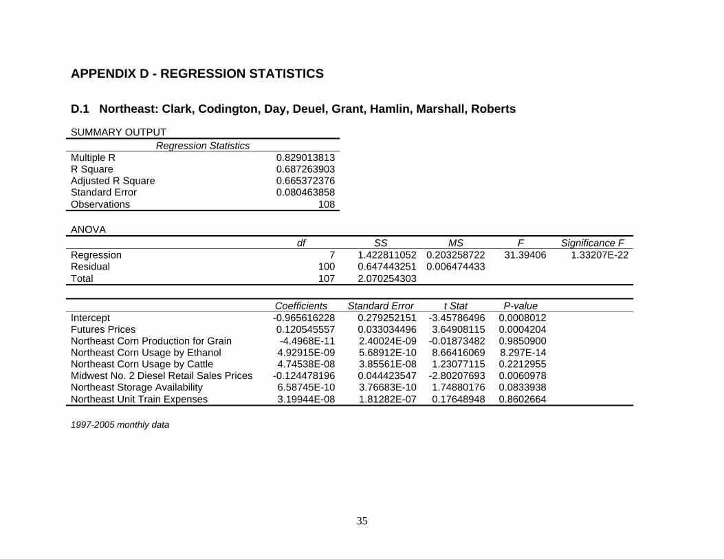
APPENDIX D - REGRESSION STATISTICS D.1 Northeast: Clark, Codington, Day, Deuel, Grant, Hamlin, Marshall, Roberts SUMMARY OUTPUT

Regression Statistics Multiple R 0.829013813 R Square 0.687263903 Adjusted R Square 0.665372376 Standard Error 0.080463858 Observations 108 ANOVA

df SS MS F Significance F Regression 7 1.422811052 0.203258722 31.39406 1.33207E-22Residual 100 0.647443251 0.006474433 Total 107 2.070254303

Coefficients Standard Error t Stat P-value Intercept -0.965616228 0.279252151 -3.45786496 0.0008012 Futures Prices 0.120545557 0.033034496 3.64908115 0.0004204 Northeast Corn Production for Grain -4.4968E-11 2.40024E-09 -0.01873482 0.9850900 Northeast Corn Usage by Ethanol 4.92915E-09 5.68912E-10 8.66416069 8.297E-14 Northeast Corn Usage by Cattle 4.74538E-08 3.85561E-08 1.23077115 0.2212955 Midwest No. 2 Diesel Retail Sales Prices -0.124478196 0.044423547 -2.80207693 0.0060978 Northeast Storage Availability 6.58745E-10 3.76683E-10 1.74880176 0.0833938 Northeast Unit Train Expenses 3.19944E-08 1.81282E-07 0.17648948 0.8602664 1997-2005 monthly data

36

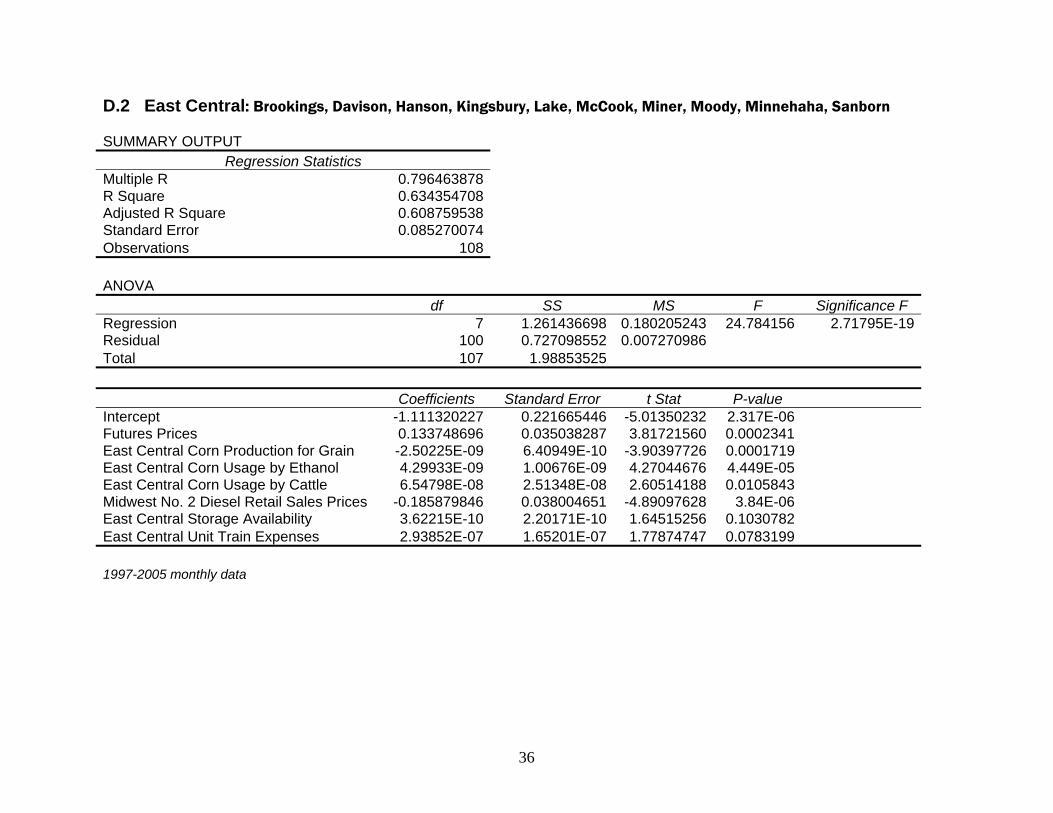
D.2 East Central: Brookings, Davison, Hanson, Kingsbury, Lake, McCook, Miner, Moody, Minnehaha, Sanborn SUMMARY OUTPUT

Regression Statistics Multiple R 0.796463878 R Square 0.634354708 Adjusted R Square 0.608759538 Standard Error 0.085270074 Observations 108 ANOVA

df SS MS F Significance F Regression 7 1.261436698 0.180205243 24.784156 2.71795E-19Residual 100 0.727098552 0.007270986 Total 107 1.98853525

Coefficients Standard Error t Stat P-value Intercept -1.111320227 0.221665446 -5.01350232 2.317E-06 Futures Prices 0.133748696 0.035038287 3.81721560 0.0002341 East Central Corn Production for Grain -2.50225E-09 6.40949E-10 -3.90397726 0.0001719 East Central Corn Usage by Ethanol 4.29933E-09 1.00676E-09 4.27044676 4.449E-05 East Central Corn Usage by Cattle 6.54798E-08 2.51348E-08 2.60514188 0.0105843 Midwest No. 2 Diesel Retail Sales Prices -0.185879846 0.038004651 -4.89097628 3.84E-06 East Central Storage Availability 3.62215E-10 2.20171E-10 1.64515256 0.1030782 East Central Unit Train Expenses 2.93852E-07 1.65201E-07 1.77874747 0.0783199 1997-2005 monthly data

37

D.3 Southeast: Bon Homme, Charles Mix, Clay, Douglas, Hutchinson, Lincoln, Turner, Union, Yankton SUMMARY OUTPUT

Regression Statistics Multiple R 0.771500429 R Square 0.595212911 Adjusted R Square 0.566877815 Standard Error 0.079846684 Observations 108 ANOVA

df SS MS F Significance F Regression 7 0.937474503 0.133924929 21.006208 3.76394E-17 Residual 100 0.6375493 0.006375493 Total 107 1.575023803

Coefficients Standard Error t Stat P-value Intercept -0.822507231 0.209276204 -3.93024728 0.00015643 Futures Prices 0.142023272 0.034237259 4.14820799 7.0420E-05 Southeast Corn Production for Grain -2.27352E-09 4.62739E-10 -4.91318287 3.5060E-06 Southeast Corn Usage by Ethanol 5.43733E-09 9.79565E-10 5.55076048 2.3428E-07 Southeast Corn Usage by Cattle 4.03345E-08 2.75315E-08 1.46503244 0.14604909 Midwest No. 2 Diesel Retail Sales Prices -0.173942106 0.036071071 -4.82220525 5.0851E-06 Southeast Storage Availability 2.68931E-10 1.95507E-10 1.37556036 0.17203122 Southeast Unit Train Expenses 8.24452E-08 4.32732E-08 1.90522711 0.05962330 1997-2005 monthly data

38

D.4 North Central: Brown, Campbell, Edmunds, Faulk, McPherson, Potter, Spink, Walworth SUMMARY OUTPUT

Regression Statistics Multiple R 0.707360165 R Square 0.500358403 Adjusted R Square 0.465383491 Standard Error 0.106850373 Observations 108 ANOVA

df SS MS F Significance F Regression 7 1.14333814 0.16333402 14.306209 9.23819E-13Residual 100 1.141700212 0.011417002 Total 107 2.285038352

Coefficients Standard Error t Stat P-value Intercept -1.606633859 0.249758118 -6.43275931 4.34951E-09 Futures Prices 0.157212916 0.045617476 3.44633086 0.00083233 North Central Corn Production for Grain -5.35683E-09 1.70297E-09 -3.14557038 0.00218353 North Central Corn Usage by Ethanol 1.08557E-08 3.23846E-09 3.35211927 0.00113309 North Central Corn Usage by Cattle 1.81439E-07 7.12949E-08 2.54490877 0.01245912 Midwest No. 2 Diesel Retail Sales Prices -0.120858405 0.052097817 -2.31983627 0.02238260 North Central Storage Availability 9.0322E-10 4.83752E-10 1.86711472 0.06481474 North Central Unit Train Expenses 1.39054E-07 9.10668E-08 1.52694873 0.12993060 1997-2005 monthly data

39

D.5 Central: Aurora, Beadle, Brule, Buffalo, Hand, Hughes, Hyde, Jerauld, Sully SUMMARY OUTPUT

Regression Statistics Multiple R 0.824878163 R Square 0.680423985 Adjusted R Square 0.658053663 Standard Error 0.084687815 Observations 108 ANOVA

df SS MS F Significance FRegression 7 1.527029028 0.218147004 30.416371 3.83519E-22Residual 100 0.717202602 0.007172026 Total 107 2.24423163

Coefficients Standard

Error t Stat P-value Intercept -0.288097266 0.25421121 -1.13329883 0.25979856 Futures Prices 0.082283799 0.03700274 2.22372180 0.02841701 Central Corn Production for Grain -8.35719E-09 1.06485E-09 -7.84824229 4.8112E-12 Central Corn Usage by Ethanol 9.08291E-09 6.92867E-09 1.31091791 0.19288797 Central Corn Usage by Cattle -1.41045E-07 6.74895E-08 -2.08987625 0.03916610 Midwest No. 2 Diesel Retail Sales Prices -0.085641598 0.03568172 -2.40015330 0.01823832 Central Storage Availability 3.39376E-10 5.53027E-10 0.61366887 0.54082759 Central Unit Train Expenses 4.46192E-07 8.75401E-08 5.09700422 1.6353E-06 1997-2005 monthly data

40

D.6 East River as whole "State" SUMMARY OUTPUT

Regression Statistics Multiple R 0.848347997 R Square 0.719694325 Adjusted R Square 0.700072927 Standard Error 0.074502657 Observations 108 ANOVA

df SS MS F Significance F Regression 7 1.425147151 0.20359245 36.679056 6.25001E-25Residual 100 0.555064589 0.005550646 Total 107 1.980211741

Coefficients Standard

Error t Stat P-value Intercept -0.578009362 0.194257254 -2.97548405 0.00366800 Futures Prices 0.07512753 0.032753101 2.29375317 0.02389684 East River Corn Production for Grain -9.38216E-10 1.66144E-10 -5.64699583 1.5357E-07 East River Corn Usage by Ethanol 2.2418E-09 2.72284E-10 8.23329978 7.1391E-13 East River Corn Usage by Cattle 1.37574E-08 6.93862E-09 1.98272501 0.05014136 Midwest No. 2 Diesel Retail Sales Prices -0.183266048 0.033704126 -5.43749594 3.8344E-07 East River Storage Availability 3.27964E-11 5.55366E-11 0.59053711 0.55616287 East River Unit Train Expenses 4.63852E-09 1.9602E-08 0.23663536 0.81342374 1997-2005 monthly data