Claremont CollegesScholarship @ Claremont

CMC Senior Theses CMC Student Scholarship

2013

The Impact of Participatory Notes on the IndianRupee Exchange RateRohan KothariClaremont McKenna College

This Open Access Senior Thesis is brought to you by Scholarship@Claremont. It has been accepted for inclusion in this collection by an authorizedadministrator. For more information, please contact scholarship@cuc.claremont.edu.

Recommended CitationKothari, Rohan, "The Impact of Participatory Notes on the Indian Rupee Exchange Rate" (2013). CMC Senior Theses. Paper 654.http://scholarship.claremont.edu/cmc_theses/654

CLAREMONT McKENNA COLLEGE

THE EFFECT OF PARTICIPATORY NOTES ON THE INDIAN RUPEE EXCHANGE RATE

SUBMITTED TO

PROFESSOR THOMAS WILLETT

AND

PROFESSOR LISA MEULBROEK

AND

DEAN GREGORY HESS

BY

ROHAN KOTHARI

FOR

SENIOR THESIS

Spring 2013

April 29, 2013

  2  

Abstract

Since 1992, India has grown as a global player in the finance world. In spite of its

success, India has not been able to rid itself of potentially harmful practices. One such practice is

the issuing of Participatory Notes (PN) to foreign investors, so that they can anonymously

purchase securities or derivatives listed on the Indian Stock Exchanges. This instrument came

into public view when it accounted for approximately 50% of all foreign portfolio assets in India.

Since then, the laws regarding PNs have evolved to become a more transparent version of the old

rules. Although PN levels are not close to as high as 2007, a rising trend in PNs has been

observed from September to November 2012. Regulation may have helped figure out who the

end PN holder is, but it has not helped mitigate the inherent volatility that some scholars argued

PNs had. This paper follows previous researchers claims to try to resolve the issue using rigorous

econometric analysis. It uses the Vector Auto Regression (VAR) Model to find the coefficient of

change in Participatory Note volume when regressed against the U.S. Dollar Indian Rupee

Nominal Exchange Rate. Although the model’s results are interpreted, a problem of serial

correlation existed in the model, thus impairing the results.

  3  

Acknowledgements

I would like to thank Claremont McKenna College for being a home, (really far) away

from home. Before I came here, I had no idea it was possible to learn, while living in North

Quad. Although, I might not leave here with a stellar academic performance, I will leave here

with a much larger, and more diverse, pool of knowledge. I will leave smarter, and much more of

a global citizen than I was before I transferred to CMC. Most importantly, I will leave here

longing to come back.

I would like to thank my teachers and professors for inculcating copious amounts of

knowledge in me, even though I’ve never understood how they did it in face of my laissez-faire

attitude. In this regard, I would like to mention Professor Meulbroek, who even though, I was

told, had an aversion to my type, still managed to cultivate a passion for finance in me.

In light of my Senior Thesis, it would be tantamount to treason if I didn’t mention the

amazing support I have gotten from the administrative staff at this school. All the way from

Dean Maraña being at my bedside even before I completely realized I was at a hospital,1 to my

cleaners Lisa and Ilma who always had my back, and Mrs. Morgan, who somehow managed to

keep track of me, and simultaneously, all the other students at school. I would also like to thank

Professor Willett for being my reader under unorthodox circumstances, and for his invaluable

input.

I would like to thank all the friends I’ve made at CMC, and the other Claremont Colleges,

for supporting me. Last, but definitely not the least, I would like to thank my parents for all the

                                                                                                               1 Sports injury

  4  

love and support they’ve given me throughout my entire life. I wouldn’t be writing this paper

without it.

  5  

Table of Contents

I. Abstract………..…………………………………………………………………. 2

II. Acknowledgements...…………………………………………………………….. 3

III. List of Abbreviations...…………………………………………………………… 6

IV. Background..……………………………………………………………………… 8

a. 1991 Balance of Payments Crisis ...……………………………………… 8

b.Post-Crisis Reforms...……………………………………………………… 10

c. Foreign Institutional Investor ...…………………………………………… 12

V. Participatory Notes...……………………………………………………………… 16

a. Regulatory Timeline.....…………………………………………………… 19

VI. Literature Review.....…………………………………………………..………….. 22

VII. Data and Methodology..…………………………………………………………… 24

VIII. Analysis ..…………………………………………………………………………. 28

IX. Discussion ..………………………………………………………………………. 33

X. Conclusion .………………………………………………………………………. 35

XI. Works Cited .……………………………………………………………………… 37

XII. Appendix A: STATA Input and Output.. ………………………………………… 39

  6  

List of Abbreviations General

1. AuC – Assets Under Custody

2. BoP – Balance of Payments

3. BSE – Bombay Stock Exchange

4. DFI – Development Finance Institutes

5. DTAA – Double Tax Avoidance Agreement

6. ECB – External Commercial Borrowings

7. FDI - Foreign Direct Investor

8. FERA – Foreign Exchange Regulation Act

9. FII – Foreign Institutional Investor

10. FVCI – Foreign Venture Capital Invesment

11. IMF - International Monetary Fund

12. INR – Indian National Rupee

13. KYC – Know Your Client

14. MoU – Memorandum of Understanding

15. NRI – Non-Resident Indian

16. NSE – National Stock Exchange

17. ODI – Overseas Derivative Instrument

18. PN – Participatory Note

19. RBI – Reserve Bank of India

20. PIO – Person of Indian Origin

21. SEBI – Securities and Exchange Board of India

  7  

22. SEC – Securities and Exchange Commision

23. QFI – Qualified Foreign Investor

24. USD – United States Dollar

Data and Analysis

1. ARCH – Autoregressive Conditional Heteroskedasticity

2. GARCH – General Autoregressive Conditional Heteroskedasticity

3. M3 – Broad Money

4. VAR – Vector Autoregression

5. USDXY – US Dollar Spot Rate Index

6. AUCNPN – Assests under FIIs, not including Participatory Notes

  8  

Background

India is a unique country in many ways. The structure of India’s economy has evolved in

a unique manner over its independent history. Politically, it has undergone an interesting

metamorphosis. Numerous kingdoms ruled India before the British colonized and unified the

country in the 19th century. After achieving independence in 1947, India decided to remain non-

aligned during the Cold War, in its quest to maintain strategic autonomy and economic

independence. This political sentiment had an immense impact on the development of India’s

economy. India’s early leaders instituted a state-controlled economic system, dubbed the

“Licence Raj”, and it existed from independence until its eventual dismantling at the end of the

Cold War in the early 1990s.

`“Licence Raj” is translated into English as the ‘rule of licenses’. The term refers to the

Soviet-inspired central planning approach that India adopted, following its independence in

1947. Although the private sector was nominally allowed to operate, it could only do so after

facing numerous regulations, permits, and quotas that together served as symbols of India’s

infamous red tape bureaucracy. Effectively, the only significant private industries in India prior

to economic liberalization were firms that were supported by the state through special licenses

and permits.

1991 Balance-of-Payments Crisis

In the 1980’s, India ushered in a period of relatively unprecedented economic growth

through a rapid escalation of public expenditure, which was financed by unsustainable

borrowing. By 1985, the Rupee began to depreciate against the dollar, boosting exports. In spite

of this jump in exports, the soaring debt caused an increase in the current account deficit from

  9  

1.7% of GDP in 1981 to 3.1% of GDP in 1989.2 In 1990, India’s exports crashed, as a result of

economic slowdowns in India’s biggest export partners. Credit started freezing up as a result of a

downgrade of government debt from investment grade to junk. India’s foreign exchange reserves

had dropped to merely 7 weeks worth of exports by mid 1990, when the Gulf War began. This

war led to a global oil supply shock, and Indian exports began to dry up. On the other hand,

petroleum imports to India increased by more than 2 billion USD.3 This exacerbation of the

current account deficit spilled over to affect the capital account. Political instability, a credit

crunch, and the current accounts crisis led to a dip in investor confidence. While investors began

to pull their money out, creditors refused to buy short-term debt, and NRIs (Non-resident

indians, or Indian expatriates), the only significant source of foreign portfolio investment at the

time, began to rapidly pull their money out of India4. This balance of payments crisis manifested

itself as the foreign exchange reserves fell to three weeks worth of imports. The urgency of this

crisis was evident when the Finance Minister told parliament that the crisis “constitutes a serious

threat to the sustainability of growth processes and orderly implementation of our development

programs.”5 In order to avoid default, India used all its gold reserves as collateral to secure a loan

of 1.8 billion dollars from the IMF in January 1991.6

The Indian government secured the IMF loan during the interim tenure of the Janata Dal

(Secular) government. Elections were scheduled for May 1991, but were delayed till June

because of the assassination of a prominent opposition candidate and former Prime Minister,

                                                                                                               2 India,  1991  Country  Economic  Memorandum.  Vol.  1.  World  Bank,  1991  3 Bery, Suman, Bosworth, Barry P. and Panagariya, Arvind. India Policy Forum 2009/10. Volume 6: Editors' Summary. Brookings Institute, July 2009 4 Cerra, Valerie, and Sweta Chaman Saxena. "What caused the 1991 currency crisis in India?." IMF Staff Papers (2002): 395-425. 5 Budget Speech 1991-92. Shri Manmohan Singh, Minister of Finance. 24th July, 1991 http://www.indiabudget.nic.in/bspeech/bs199192.pdf 6 India,  1991  Country  Economic  Memorandum.  Vol.  1.  World  Bank,  1991

  10  

Rajiv Gandhi. In June, the minority coalition government of P.V. Narasimha Rao was elected,

and it pioneered sweeping reforms under its new Finance Minister, the economist and former

RBI governor, Dr. Manmohan Singh. Although some of the improvements were covenants of the

IMF loan, the government indicated its intention to bring about an era of liberalization in all

sectors of the economy, including crucially, in the financial sector.

 

Post-Crisis Reforms

In order to comply with the IMF’s Balance of Payments Manual, India was forced to

undertake many important changes in its fiscal and monetary policy. The High Level Committee

on Balance of Payments (henceforth Rangarajan Committee) and the Committee on Financial

Sector Reforms (henceforth Narasimham Committee), were set up to leverage these changes to

create a strategy for future growth. To rebuild foreign exchange reserves, and begin the

implementation of market reforms, the new government devalued the Rupee by 23% against the

dollar.7 The Rangarajan committee suggested the introduction of a floating exchange rate, and

current account convertibility. As recommended by the Narasimham committee, the government

also decided to deregulate interest rates, and allowed prices to be determined by the market.

Credit controls were withdrawn, and there was a decrease in the reserve requirements.8

Entrepreneurship was allowed to thrive when the barriers to entry were lowered, even though

many industries remained under government control. The financial industry was given special

attention because of its central role in promoting investment to drive future growth. The state-

owned banks were consolidated, and Development Finance Institutes that supplied directed

                                                                                                               7 India,  1991  Country  Economic  Memorandum.  Vol.  1.  World  Bank,  1991 8 Bhasin, Niti. Banking and financial markets in India, 1947 to 2007. New Century Publications, 2007.

  11  

credit were abolished or converted into commercial banks. This paved the way for increased

private competition, and the entry of foreign banks. Foreign investment in India was encouraged

as a result of more conducive laws, lower barriers to entry, and the convertible Rupee. For

example, foreign controlling interest of businesses in India was allowed, for the first time, in

high priority industries and export driven companies.9 In November 1992, the National Stock

Exchange (NSE) was incorporated in order to implement international best practices in

secondary markets. The NSE provided investors exposure to Capital Markets (Equity) and

Wholesale Debt Markets. The Narasimham committee recommended that the Reserve Bank of

India be made the sole monetary and banking authority, independent of government intervention.

In order to ensure well-rounded reforms, a recently set up regulatory body was given full

statutory power under the Securities and Exchange Board of India (SEBI) Act of 1992. SEBI’s

role was modeled on the United States’ SEC, with a function to “protect the interests of investors

in securities and to promote the development of, and to regulate the securities market.”10

Since the effort to introduce free market policies in India, there have been incremental

changes in the structure of the financial sector. Today it is a curious contradiction between

international best practices and archaic rules. Although India is still an emerging market, some

ascribe its step-by-step growth strategy to its resilience against global financial crises. On the

other hand, the continuing lack of transparency in certain peculiar financial instruments has

served as a conduit for political corruption. This paper examines the effect of one such opaque

instrument, Participatory Notes. The next section discusses the prime users of these instruments,

Foreign Institutional Investors.

                                                                                                               9 Budget Speech 1991-92. Shri Manmohan Singh, Minister of Finance. 24th July, 1991 http://www.indiabudget.nic.in/bspeech/bs199192.pdf 10 The Securities and Exchange Board of India Act (1992), www.sebi.gov.in/acts/act15ac.pdf

  12  

Foreign Institutional Investor (FII)

After the collapse of the “Licence Raj”, India realized that it was time to globalize. In his

1991 interim budget speech, Finance Minister Dr. Manmohan Singh said, “we have now reached

a stage in development where we should welcome, rather than fear, foreign investment.”11

Although the official commencement date was 14th September 1992, FII inflows began in

January 1993.12

Today, there are multiple avenues for foreigners to invest in India. These can be

categorized as Direct Investment, Portfolio Investment, Depository Receipts, External

Commercial Borrowing (ECB), and External Assistance.

Direct Investment is defined as equity investments in Indian companies without using the stock

markets. It is divided into investments in listed companies, called Foreign Direct Investment

(FDI), and unlisted companies called Foreign Venture Capital Investment (FVCI). FDI can be

subdivided into two investment routes, the Automatic Route and the Government Route. As one

can infer from their names, the latter requires approval from the Government whereas the former

has pre-existing procedures for investment. Depository Receipts are derivatives that map the

movement of Indian stocks on foreign stock exchanges. Indian companies issue these receipts,

which do not have any end-user restrictions. ECB is method of investment that allows Indian

companies, both private and public, to raise money internationally. This includes bank loans,

trade credit, and other securitized instruments. External Assistance is aid that India receives from

foreign governments. Portfolio Investment is defined as investments in India through the stock

market or mutual funds. There are three classifications of portfolio investors. The first, and

                                                                                                               11 Budget Speech 1991-92. Shri Manmohan Singh, Minister of Finance. 24th July, 1991 http://www.indiabudget.nic.in/bspeech/bs199192.pdf 12 Indian Securities Market Volume XIV 2011, www.nseindia.com/content/us/ismr_full2011.pdf

  13  

newest is a Qualified Foreign Investor (QFI). QFIs are defined as non-Indians who are residents

of Financial Action Task Force countries, and are required to have a Memorandum of

Understanding (MoU) with SEBI through their country.13 This is a recently introduced catchall

category for individuals who are not registered through other routes, but can accept Indian tax

obligations.14 The second type of investor is a Non-Resident Indian (NRI) or a Person of Indian

Origin (PIO). The Indian government officially assigns these self-explanatory terms to people

who possess NRI or PIO identification cards. People from both these categories are allowed to

own a maximum of 5% of an Indian company.15 They are also allowed to invest in government

securities and corporate debt.

The third, and biggest category by Assets Under Custody (AuC), is the Foreign

Institutional Investor (FII). In order to be considered as an FII, applicants need to have a proven

track record and be overseen by their respective regulatory authority. Although there are

exceptions to that rule, FII’s are generally one of the following institutions: university funds,

endowments, foundations, charitable trusts, pension funds, mutual funds, investment trusts,

insurance firms, reinsurance firms, international or multilateral organizations or one of its

agencies, or a Foreign Governmental Agency. It could also be “an asset management company,

investment manager or advisor, bank or institutional portfolio manager, established or

incorporated outside India and proposing to make investments in India on behalf of broad based

funds16 and its proprietary funds, if any.”17 As of the 30th of November 2012, 1752 FII’s are

                                                                                                               13 RBI FAQ, http://www.rbi.org.in/scripts/FAQView.aspx?Id=26 14 ibid 15 ibid 16 Broad based fund is defined as one with a minimum of 20 investors, in which the majority shareholder owns less than 49% 17 Securities And Exchange Board Of India (Foreign Institutional Investors) Regulations, 1995. www.sebi.gov.in/acts/act07a.html

  14  

registered with SEBI.18 Not only do FIIs trade for themselves, but they also trade for their

clients, who are known as sub-accounts. These sub-accounts do not have to be regulated to be

able to register with SEBI. On the contrary, High Net Worth (over $ 50 mil)19 Individuals can

register as sub-accounts. On November 30th 2012, SEBI had 6306 sub-accounts registered.

SEBI limits and regulations on FIIs have been amended and relaxed over time. In 1998

FIIs were first allowed access to the debt market. There are also some restrictions on the

investments that FIIs, and their sub-accounts, can make. Foreign Corporates and Foreign

Individuals are allowed to invest up to 5% of a company’s paid-up capital. FIIs are allowed to

invest 10% for themselves, and for all the other types of sub-accounts. Including all their sub-

accounts, FIIs are not allowed to hold more than 24% of the total firm capital.20 This limit can be

lifted up to the statutory limit, on the behest of the Board of Directors of the company in

question. As of today, there are over 290 Indian companies in which FIIs own over 30% of the

paid-up capital.21

                                                                                                               18 http://www.sebi.gov.in/sebiweb/investment/FIITrendsNew.jsp 19 Securities And Exchange Board Of India (Foreign Institutional Investors) Regulations, 1995. www.sebi.gov.in/acts/act07a.html 20 Indian Securities Market Volume XIV 2011, www.nseindia.com/content/us/ismr_full2011.pdf 21 List of Foreign Investment in Indian Companies. RBI. http://www.rbi.org.in/scripts/BS_FiiUSer.aspx

  15  

22

                                                                                                               22  Indian Securities Market Volume XIV 2011, www.nseindia.com/content/us/ismr_full2011.pdf  

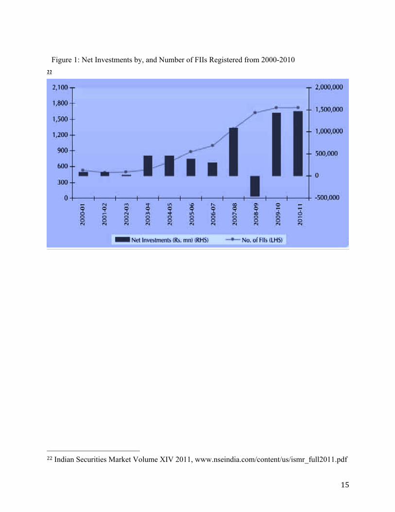
Figure 1: Net Investments by, and Number of FIIs Registered from 2000-2010

  16  

Participatory Notes (PN)

In December 2007, Assets under Management of FIIs nearly doubled year-over-year.

Although this would normally be a reason to rejoice, almost 50% of FII flows in the previous

two years were through an opaque financial instrument known as a Participatory Note. This

section introduces and defines this instrument, and weighs its advantages against its

disadvantages. 23

PNs are a type of Offshore Derivative Instrument (ODI), and are unique to a few Asian

countries, including India. The SEBI (FII) Regulations defines an ODI as an instrument “which

is issued overseas by a foreign institutional investor against securities held by it that are listed or

proposed to be listed on any recognised stock exchange in India.”24 These ODIs can also be

issued against derivatives, resulting in leveraged exposure to the Indian Stock Market. 25

Although there are other ODIs like equity-linked notes and capped return notes, PNs are the most

common type of ODI.26

PNs became a conduit for international investment in India since their inception around

1992.27 In spite of the fact that the official rules on FIIs were released in 1995, these instruments

were attractive for investors who were apprehensive, yet interested to enter the emerging Indian

market. Theses instruments provide easy access to the Indian market. If an investor would like to

                                                                                                               23 Mohan, TT Ram. "Neither Dread Nor Encourage Them." Economic and Political Weekly (2006): 95-99. 24 Securities And Exchange Board Of India (Foreign Institutional Investors) Regulations, 1995. www.sebi.gov.in/acts/act07a.html 25 Lokeshwarri S.K. “The Fading Allure Of P-Notes.” Business Daily. January 28, 2011 26 Indian Securities Market Volume XIV 2011, www.nseindia.com/content/us/ismr_full2011.pdf, pg188 27 Singh, Manmohan. Use of Participatory Notes in Indian Equity Markets and Recent Regulatory Changes. Vol. 7. International Monetary Fund, 2007.

  17  

buy securities or derivatives, he sends his order to the FII. This FII then conveys that order to his

broker in India, who actually buys the securities. In return, PNs are issued to the FII, who then

passes them on to its clients. 28 Apart from its ease of use, there are other factors that made a case

for the creation of PNs. These instruments were freely tradable, which provided liquidity in the

market.29 This liquidity was much required in the recently and partially liberalized Indian

market. Participatory Notes provided a method for Mauritian individuals and companies to take

advantage of the zero Capital Gains Tax accorded by the Double Taxation Avoidance Agreement

(DTAA).30 Investing through this instrument also significantly lowered the cost of entry into the

Indian markets. Some of these costs include, the money required to establish broker or bank

relations, costs associated with FII registration and subsequent disclosures, and costs associated

with foreign exchange.31

In the context of the aforementioned cost advantages over FIIs, one can deduce the higher

premium of an individual transaction through PNs versus FIIs.32 Similarly, some of the other

advantages of PNs are just one side of a double-edged sword.

The first issue with PNs was the capital gains tax arbitrage opportunities that were

created as a result of the DTAA. Onshore investors had to pay taxes up to 40% on short-term

capital gains, compared to 0% in Mauritius. This led to an increase in the number of offshore

                                                                                                               28 N., Nikhil Kumar, Implications of Hedge Funds on the Indian Capital Market (August 20, 2007) 29 “White Paper on Black Money.” Ministry of Finance, Department of Revenue, India. 2012, pg 27 30 Singh, Manmohan. Use of Participatory Notes in Indian Equity Markets and Recent Regulatory Changes. Vol. 7. International Monetary Fund, 2007. 31 Report of the Expert Group on Encouraging FII Flows and Checking the Vulnerability of Capital Markets to Speculative Flows, Government of India, Ministry of Finance, Department of Economic Affairs, New Delhi, November 2005 (also, Lahiri Committee), pg 16 32 N., Nikhil Kumar, Implications of Hedge Funds on the Indian Capital Market (August 20, 2007)

  18  

firms that registered in the country. Additionally, certified residents of Mauritius also had to pay

minimal corporate tax, and therefore companies began routing their investments in India through

Mauritius. 33 Between April 2000 and March 2011, Mauritius (41.8%) and Singapore (9.17%)

accounted for over half of the cumulative FDI in India.34 These disproportionate inflows occur

even though 8 years of the data set is cut out, and some arbitrage opportunities were nullified by

2004, through the decrease in the tax rate on Indian onshore Capital Gains and the increase in the

cost of setting up an establishment in Mauritius.35

An organization that was against PNs from the start was the RBI. In its dissent of the

Expert Group on FIIs, the RBI suggested winding down all PNs and ceasing further issues. They

said that the suspicious and anonymous nature of the cash flows should be reason enough to shut

PNs down. The anonymity could get further magnified once PNs are traded between foreign

investors through a process they call “multi-layering.”36 This made it almost impossible to

monitor entry into the Indian Market. In 2004, SEBI passed directives to curb these issues. They

decreed that PNs could only be issued to regulated bodies. However, it was downplayed as a

mere strengthening of Know Your Client (KYC) norms.37 SEBI rejected RBI’s proposal to ban

PNs because they believed the financial community would have seen it as a recessive measure.38

One problem that the government did not fix during the 2004 amendment was the

plausibility of “Round-tripping.” Round-tripping is the process by which tax-free illicit or black

                                                                                                               33 Singh, Manmohan. Use of Participatory Notes in Indian Equity Markets and Recent Regulatory Changes. Vol. 7. International Monetary Fund, 2007. 34 “White Paper on Black Money.” Ministry of Finance, Department of Revenue, India. 2012. 35 Singh, Manmohan. Use of Participatory Notes in Indian Equity Markets and Recent Regulatory Changes. Vol. 7. International Monetary Fund, 2007. 36 RBIs dissent to EG. “White Paper on Black Money.” Ministry of Finance, Department of Revenue, India. 2012. Annex IV 37 Press Release, Securities and Exchange Board of India, January 23rd, 2004 38 Vasudevan, A. "A Note on Portfolio Flows into India." Economic and Political Weekly (2006): 90-92.

  19  

money leaves India through illegal routes, and is then repatriated to the country with minimal

fees. Since the official definition of regulated bodies includes an “individual or entity”39 whose

investment advisory is regulated, PNs provide a perfect path to bring prodigal money back into

the country. The least probable issue, although still plausible, is the use of PNs by terrorists.

High net worth terrorists could purchase PNs through their asset managers, and then gift the

notes as payment, without paying any tax on the transfer. In spite of a longitudinal cross-section

of society raising concerns about Participatory Notes, they are still traded in the market today.

Therefore, to completely understand the situation today, it is important to be cognizant of the

regulatory past.

Regulatory timeline

Participatory notes have caused friction with regulators in the countries that it exists.

Taiwan introduced strong disclosure requirements for PNs in December 1999, but they rescinded

those regulations 6 months later.40 The rules on PNs in India have been shaped by the regulatory

changes in the past. The idea of an offshore instrument for investment in Indian securities

probably stems from the Double Taxation Avoidance Agreement with Mauritius. However, PNs

first came into existence when the economy opened up in 1992.41 In conjunction with the

Foreign Exchange Regulation Act (FERA) of 1973, the Government of India guidelines released

                                                                                                               39 Singh, Manmohan. Use of Participatory Notes in Indian Equity Markets and Recent Regulatory Changes. Vol. 7. International Monetary Fund, 2007. Appendix II 40 Report of the Expert Group on Encouraging FII Flows and Checking the Vulnerability of Capital Markets to Speculative Flows, Government of India, Ministry of Finance, Department of Economic Affairs, New Delhi, November 2005 (also, Lahiri Committee), pg 45 41 Singh, Manmohan. Use of Participatory Notes in Indian Equity Markets and Recent Regulatory Changes. Vol. 7. International Monetary Fund, 2007.

  20  

on 14th September 1992 provided a framework for foreign investment in India.42 The official

guidelines for PNs came out in 1995 as part of SEBIs rules on FIIs.

Since then there have been a number of amendments to the rules, but only a few of them have

significantly affected PNs.

The first major amendment was probably made in January 2004. The RBI had voiced its

issues with PNs in 2003. It believed that the opacity, and the ease of acquiring, of these

instruments created more risk than benefit for the economic stability of India. Since the end-user

of this instrument was unknown, it could be used not only for fraudulent purposes but also for

malicious purposes, as detailed above. In order to alleviate these qualms, SEBI decided to install

robust Know Your Customer (KYC) norms. They also stipulated that FIIs could only issue them

to other “regulated”43 entities. In spite of these changes, the PN volumes continued to rise until

more than half of FII assets were in the form of PNs. These high volumes proved a cause for

concern because PNs were highly attractive instruments even though SEBI controlled the

anonymity of the instrument. The increase in companies routing their investments through

Mauritius alluded to the fact that investors were taking advantage of the tax arbitrage

opportunities presented by PNs. Regulators were also worried simply about the high volumes,

because a mass international exodus from the Indian stock markets could have a major impact on

the market, possibly affecting domestic investor confidence. On October 26th, 2007, SEBI issued

a statement in regard to curbing PN flows. These measures were implemented in the amendment

made on 22nd May 2008. There were three fundamental changes these measures made. Firstly,

sub-accounts were disallowed from issuing PNs. Secondly, PNs on derivatives had to be

                                                                                                               42 Indian Securities Market Volume XIV 2011, www.nseindia.com/content/us/ismr_full2011.pdf 43 Singh, Manmohan. Use of Participatory Notes in Indian Equity Markets and Recent Regulatory Changes. Vol. 7. International Monetary Fund, 2007.

  21  

completely wound up by 2009. Thirdly, there was a 40% ceiling imposed on PNs as a percent of

the total AuC. Fourthly, companies that were below this ceiling were allowed to increase their

percentage of PNs by a maximum of 5% each year.44 These complicated norms created a sense

of unease within foreign investors, and they began to offload more than just their PNs issued on

derivatives. Although this could be explained as the unraveling of derivative included strategies

such as a Protective Put, SEBI decided to rectify the changes made in May. Apart from sub-

accounts not being able to issue PNs, all other changes were revoked. 45 In 2012 the government

decided to cut down the time lag on reporting PN transactions from 6 months to 10 days.

Although PNs are not close to the levels of 2007, they have been increasing in numbers

recently. In light of this fact, it is important to understand the effects of this instrument on the

stability of the Indian Rupee.

                                                                                                               44 Securities And Exchange Board Of India (Foreign Institutional Investors) Regulations amendment 22nd May, 2008. www.sebi.gov.in/acts/act07a.html 45 Securities And Exchange Board Of India (Foreign Institutional Investors) Regulations amendment 10th Oct, 2008. www.sebi.gov.in/acts/act07a.html

  22  

Literature Review

The Narasimham committee of 1991 suggested against allowing investments from NRIs

because of the volatility associated with those cash flows.46 However, they offer no empirical

evidence confirming this volatility. The Narasimham committee suggested against NRI flows out

of skepticism caused by the mass outflow of NRI investments right before the 1992 Balance of

Payments crisis. Ironically, instruments still exist today, which could have more volatile cash

flows than the NRI flows. Before we understand the effects of those specific instruments, it is

important to understand the overarching effects of FIIs on the Indian stock market. Rai and

Bhanumurthy47 used monthly data to determine that equity returns are the main determinants of

FII investment. Dhiman48 confirmed their findings when he concluded that the average daily

returns of the NSE granger caused the daily purchase to sales ratio of FIIs. Mohan49 pointed out

that FII flows accounted for 69% of all foreign investment in India, as compared to an average of

20% for developing countries. He predicted that FII flows were more volatile than FDI flows,

thus leading to a greater relative volatility in Indian markets as compared to other emerging

markets. However, using an event study methodology in his other study, Mohan50 found that on

the contrary FII flow volatility did not systematically affect the stock market. He cited the “Black

Monday” crash of May 2004 when the stock market was resilient to an eight-sigma volatility, in

                                                                                                               46 Bhasin, Niti. Banking and financial markets in India, 1947 to 2007. New Century Publications, 2007. 47 Rai, Kulwant, and N. R. Bhanumurthy. "Determinants of foreign institutional investment in India: The role of return, risk, and inflation." The Developing Economies 42.4 (2004): 479-493. 48 Dhiman, Rahul. “Impact Of Foreign Institutional Investor On The Stock Market” International Journal in Research of Finance and Marketing 2.4 (2012):32-46. 49  Mohan, TT Ram. "Stock market fall: Managing volatile flows." Economic and Political Weekly (2006): 2411-2413. 50  Mohan, TT Ram. "Neither Dread Nor Encourage Them." Economic and Political Weekly (2006): 95-99.

  23  

spite of FII outflows. Therefore it seems that FII outflows do not create enough instability to

result in a mass sell-of in the Indian market.

The one way that FIIs create weakness in the Indian economy is through the exchange

rate. According to Chandrasekhar51 large FII inflows lead to an appreciation of the Rupee,

hurting the exports of the country, even though it makes imports cheaper. Conversely, large FII

outflows depreciate the value of the Rupee, increasing exports and making imports more

expensive. In order to mitigate the rise in Rupee, the RBI buys foreign exchange. However, this

affects their ability to control domestic money supply. In order to avoid this problem, before

2006, the RBI would sell government securities equal to the value of foreign exchange

purchased. The Lahiri Report52 raises concerns about the enhanced volatility of PN flows. It

claims that individuals, who determine their own entry and exit and usually have shorter

investment horizons than investment funds, are able to hold PNs. Further, Singh53 states that

regulators attribute the cause of the May 2004 and the May/June 2006 FII sell-offs to an initial

sell-off from PN investors.

As a result of its ability to drive other FII flows, PN flows should contribute to a greater

change in the Indian Rupee exchange rate than other FII inflows. Vasudevan54 states that there

has been no empirical analysis done on the vulnerability of PN cash flows, but unfortunately

                                                                                                               51  Chandrasekhar, C. P. "Courting Risk: Policy Manoeuvres on FII Inflows." Economic and Political Weekly (2006): 92-95. 52  Report of the Expert Group on Encouraging FII Flows and Checking the Vulnerability of Capital Markets to Speculative Flows, Government of India, Ministry of Finance, Department of Economic Affairs, New Delhi, November 2005 (also, Lahiri Committee) 53  Singh, Manmohan. Use of Participatory Notes in Indian Equity Markets and Recent Regulatory Changes. Vol. 7. International Monetary Fund, 2007.  54  Vasudevan, A. "A Note on Portfolio Flows into India." Economic and Political Weekly (2006): 90-92.

  24  

doesn’t go on to do any himself. There is very little research about the effect of PNs, specifically,

on the Indian Rupee.

The aim of this paper is to clarify the beliefs about PNs and verify whether it truly creates

more exchange rate volatility than other FII flows.

  25  

Data and Methodology

The data used in this empirical study is monthly time-series data from September 2003 to

September 2012. Monthly data was used over quarterly or yearly data because it was the highest

frequency of data that was available. This high frequency of data was preferred because it maps

the regulatory changes and the movement of the exchange rate as closely as possible. The

variables involved in this empirical study are described below. These variables were selected to

try and explain the movement of the exchange rate while controlling for confounding factors.

Individual descriptions and details for the variables are stated below.

United States Dollar/Indian Rupee Exchange Rate (USDINR):

This variable is the nominal exchange rate between the US Dollar and the Indian Rupee.

It was sourced from the Global Financial Database. It is the dependent variable in the regression.

It would be an appropriate measure of currency strength because the performance of the Indian

Rupee is practically always compared to the US Dollar. Similarly, it is also preferred to the real

exchange rate because the nominal exchange rate decides transactions. It was preferred to the

trade-weighted exchange rate because it is easier to isolate all other effects of just one country,

and hence understand the variables that affect the strength of the INR. The change in USDINR

was calculated using the following formula:

𝑐ℎ𝑈𝑆𝐷𝐼𝑁𝑅 = 𝑙𝑛𝑈𝑆𝐷𝐼𝑁𝑅!𝑙𝑛𝑈𝑆𝐷𝐼𝑁𝑅!!!

− 1

where m is the current month. Closing values at month-end were used.

  26  

United States Dollar Spot Index (USDXY):

USDINR can be affected by changes in both India and the United States. Therefore, the

USDXY variable is introduced to control against changes in the US Dollar. This variable

represents the index that measures the strength of the US Dollar against a basket of six other

major currencies, not including the Indian Rupee. The change in USDXY was calculated using

the following formula:

𝑐ℎ𝑈𝑆𝐷𝑋𝑌 = 𝑙𝑛𝑈𝑆𝐷𝑋𝑌!𝑙𝑛𝑈𝑆𝐷𝑋𝑌!!!

− 1

where m is the current month. Closing values at month-end were used.

Consumer Price Index (CPI):

CPI is the total value of the average basket of goods required by a consumer. The percent

change in this number relates to the Inflation for the country. This variable is used to measure

the real effects on the dependent variable, separate from inflation. Data for this was sourced from

the Bureau of Labor Statistics for the United States and from the Labour Bureau for India.

Inflation is given by the formula:

𝐼𝑛𝑓𝑙𝑎𝑡𝑖𝑜𝑛 =𝐶𝑃𝐼!𝐶𝑃𝐼!!!

− 1

where m is the current month. Closing values at month-end were used.

Total Value of Participatory Notes (TVPN):

This variable represents the total monetary value of PNs in Rupees Crore (10 million). It

is the most important independent variable in this regression. This variable was the restricting

variable in the regression, because data was only available from September 2003 onwards. This

  27  

data was derived from the SEBI website. The change in TVPN was calculated using the

following formula:

𝑐ℎ𝑇𝑉𝑃𝑁 =𝑙𝑛𝑇𝑉𝑃𝑁!𝑙𝑛𝑇𝑉𝑃𝑁!!!

− 1

where m is the current month. This change represents the net PN flows each month.

Assets under Custody, Foreign Institutional Investors (AUCFII):

This variable represents the total value of Assets Under FII Custody. The data for this

variable is also sourced from the SEBI website, and has the same restriction as the data for

TVPN.

AUCFII excluding PNs (AUCNPN):

This variable is derived by following formula: 𝐴𝑈𝐶𝑁𝑃𝑁 = 𝐴𝑈𝐶𝐹𝐼𝐼 − 𝑇𝑉𝑃𝑁

Since it is formed from restricting variables, AUCNPN is also restricted. It is used in this specific

way in order to view all other FII investments as separate from PN investments.

The change in AUCNPN was calculated using the following formula:

𝑐ℎ𝐴𝑈𝐶𝑁𝑃𝑁 =𝑙𝑛𝐴𝑈𝐶𝑁𝑃𝑁!𝑙𝑛𝐴𝑈𝐶𝑁𝑃𝑁!!!

− 1

where m is the current month. Similar to TVPN, the change represents the net AUCNPN flows

for each month.

Broad Money (M3):

Broad Money is defined as the sum of currency with the public, demand deposits time

deposits and other deposits with the RBI. An increase in broad money increases the Rupee

  28  

supply in the Market, and vice versa. The change in Reserve was calculated using the following

formula:

𝑐ℎ𝑀3 = 𝑙𝑛𝑀3!𝑙𝑛𝑀3!!!

− 1

where m is the current month. The data was sourced from the online RBI database.

RBI Government Securities Turnover (RBI):

Open Market Operations are the market operations conducted by the Reserve Bank of

India by way of sale/ purchase of Government securities to/ from the market with an objective to

adjust the rupee liquidity conditions in the market on a durable basis. 55 A sale of securities

increases the Rupee liquidity in the Market, and vice versa. This variable takes into consideration

the effect of sterilization mentioned in the PN section. The absolute value of turnover was used,

and the data was sourced from the online RBI database.

Note: Broad Money and government securities turnover is reported every week and thus there is

lead or lag in the time of the data by 1-2 days. However, I do not perceive this to be a big issue,

because the securities are sold every Wednesday, and the data is reported every Friday.

                                                                                                               55 RBI FAQs - http://www.rbi.org.in/scripts/FAQView.aspx?Id=79#

  29  

.

dRBI 108 -.3507408 93.57357 -329 480.24 RBI 109 54.81645 102.3259 .35 542.79 dInflation 108 .0000433 .0119457 -.0407474 .0389292 Inflation 109 .0060322 .0092756 -.0389292 .0457516 dchM3 108 -3.85e-07 .0015368 -.0052324 .003895 chM3 109 .0012645 .0010606 -.000453 .0056467 chAUCNPN 109 .0019653 .0075043 -.0229478 .0211312 chTVPN 109 .0016573 .0113841 -.035618 .03202 chUSDXY 109 -.0002915 .0058287 -.0153525 .0171213 chUSDINR 109 .0003673 .0063485 -.0172543 .0177713 Variable Obs Mean Std. Dev. Min Max

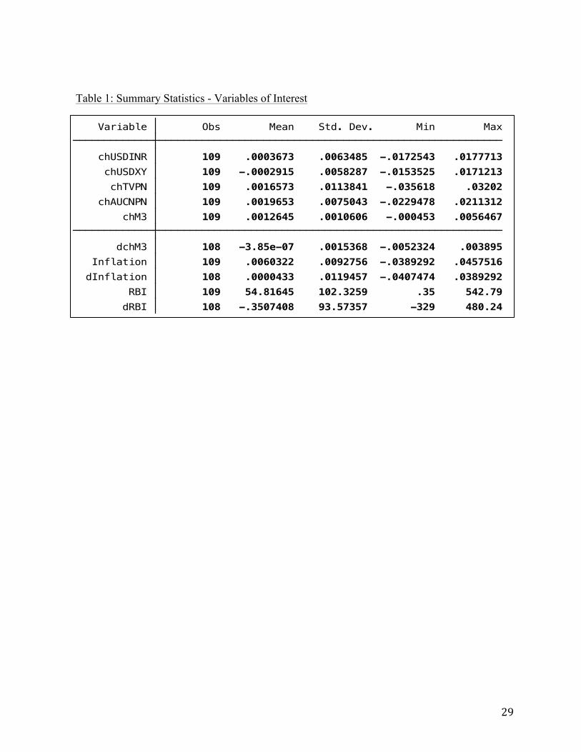
Table 1: Summary Statistics - Variables of Interest

  30  

Analysis

Note: Appendix A is a STATA supplement to the analysis.

One of the first tests that needs to be conducted with time-series data is a test for

stationary data. This kind of test is also called a unit root test. A unit root occurs when a specific

event in history creates a systematic effect on the regressand. If this effect is not controlled for, a

“spurious” regression could occur. This could manifest itself as a high R2, even if the variables

are uncorrelated.

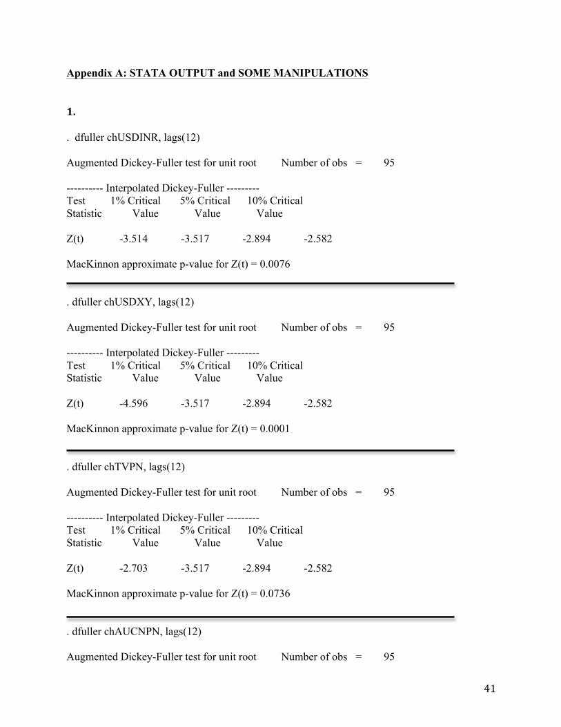
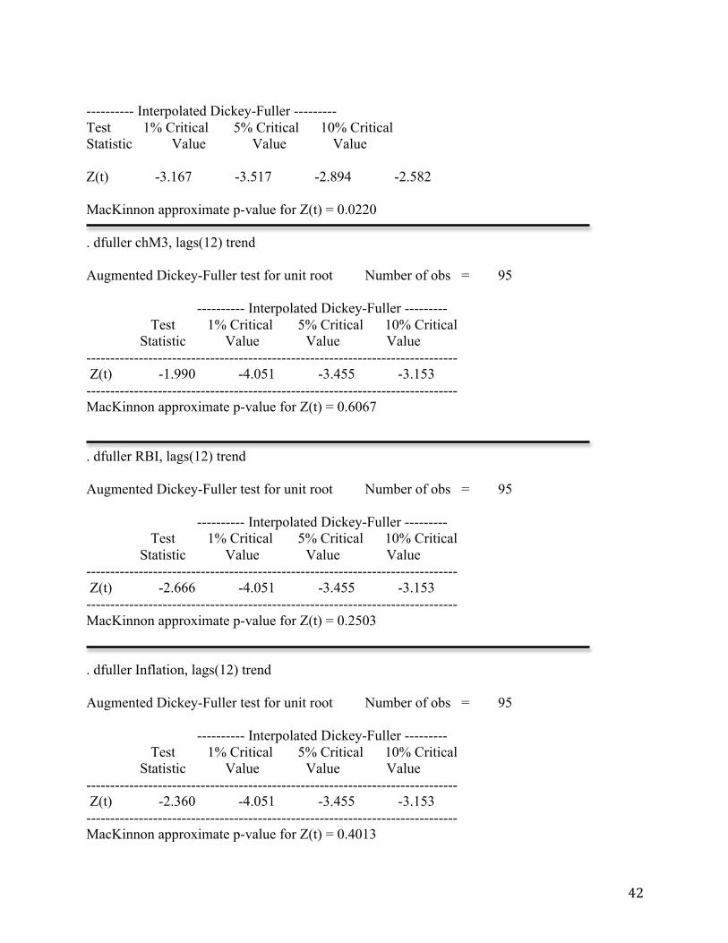
In order to check for this problem, an Augmented Dickey-Fuller test was performed. This

test is preferred to the basic Dickey-Fuller test because it takes into consideration the lagged

changes in in the variable. Since the data had monthly frequency, a lag of 12 periods was used.

The null hypothesis was that a unit root exists, and the alternative hypothesis stated that it didn’t

exist.

Table 2: Augmented Dickey-Fuller Test Results

Number Variable Test Statistic MacKinnon

P-Value

Stationary

1 chUSDINR -3.514 0.0076 Yes

2 chUSDXY -4.596 0.0001 Yes

3 chTVPN -2.703 0.0736 Yes

4 chAUCNPN -3.167 0.0220 Yes

5 chM3 -1.990 0.6067 No

6 RBI -2.666 0.2503 No

7 Inflation -2.360 0.4013 No

  31  

The test was significant at the 5% threshold and thus I rejected the null hypothesis for variables

1-4. However, we failed to reject the null for variables 5-7, and the data was not stationary. In

order to try and obtain stationary data for chM3, RBI, and Inflation, I created first differenced

variables using STATA, for each one. The first difference eliminates the effect of the unit root

because the persisting change between the two numbers is eliminated. The Augmented Dickey-

Fuller test was run again on those differenced variables, and the results were as follows:

Table 3: Augmented Dickey-Fuller Test after First Differencing

Number Variable Test Statistic MacKinnon P-

Value

Stationary

1 dchM3 -6.988 0.0000 Yes

2 dRBI -4.480 0.0002 Yes

3 dInflation -5.852 0.0000 Yes

These first-differenced variables were significantly stationary at the 1% critical level. In order to

try and decide how to proceed, one can try and examine the volatility distribution of the

regressand. To meet this, chUSDINR was regressed against the other six dependent variables

according to the following equation:

𝑐ℎ𝑈𝑆𝐷𝐼𝑁𝑅 =  𝛽! +  𝛽! ∗ 𝑐ℎ𝑈𝑆𝐷𝑋𝑌 + 𝛽! ∗ 𝑐ℎ𝑇𝑉𝑃𝑁 + 𝛽!

∗ 𝑐ℎ𝐴𝑈𝐶𝑁𝑃𝑁 + 𝛽! ∗ 𝑑𝑐ℎ𝑀3+ 𝛽! ∗ 𝑑𝑅𝐵𝐼 + 𝛽!

∗ 𝑑𝐼𝑛𝑓𝑙𝑎𝑡𝑖𝑜𝑛 + 𝑢

and then u was plot against Months.

  32  

From this graph, it didn’t look like error volatility was clustered or conditionally heteroskedastic.

However, this can be evaluated through a post-test. Out of the three vertical separators, the one

on the left is for October 2007, which is when a PN and FII sell-off was triggered when the

Indian Government announced they were going to cap the value of PNs and completely ban the

sale of PNs on derivatives. The middle line represents when the government withdrew the

measures in October 2008, and the one to the right represents the month after the United States

“officially”56 came out of its recession. I expected that the exchange rate volatility would have

been larger between the first two bands as a result of the fragile state of the U.S. economy and

foreign inflows into India. Although there is an increase in volatility, the presence of the

USDXY variable probably mitigated the clustering effect. Therefore I decided against using                                                                                                                56  According  to  the  National  Bureau  of  Economic  Research  

Figure  2:  A  plot  of  the  Residuals  against  their  Months  

  33  

Autoregressive Conditional Hetereoskedasticity (ARCH) or General Autoregressive Conditional

Hetereoskedasticity (GARCH) models to begin to fit my data.

The next logical step was to try and use the Vector Auto Regression (VAR) model. The

VAR model compares each variable and its lags to all the other variables and their lags. This

model is a powerful analytic tool just because it allows observation of multiple interactions.

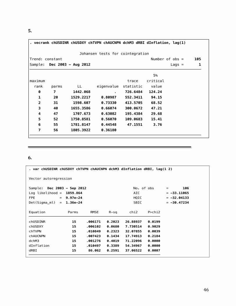
However, before running a VAR, it is important to ensure that there is no co-integration between

any two series over time. Just like non-stationary data, co-integrated time series data could lead

to a “spurious” regression. To prevent this from occurring, a Johansen test was administered, for

which the lag had to be determined. The “varsoc” function was used in STATA to generate

Akaike’s Information Criterion (AIC) and establish the lag as 1. The Johansen test was

subsequently performed, with the null hypothesis stating that the time series’ were not co-

integrated. The resulting trace statistic exceeded 5% for all ranks, and therefore we failed to

reject the null hypothesis. The series’ were not co-integrated, and therefore the unrestricted VAR

model could be implemented using a lag of 1 and 2. STATA created a system of 105 equations,

in which each variable was regressed against 1 lag and 2 lags of all the other variables, and a

constant. The VAR came up with several significant coefficients, some of which stood out. Four

separate variables were correlated with chAUCNPN, which I thought was interesting because it

alludes to the fact that the institutionalized investeor develops his data from multiple sources. I

also found it interesting that as expected, inflation and sometimes lagged inflation correlated

with the change in USDINR and the change in M3. However, both these inferences were

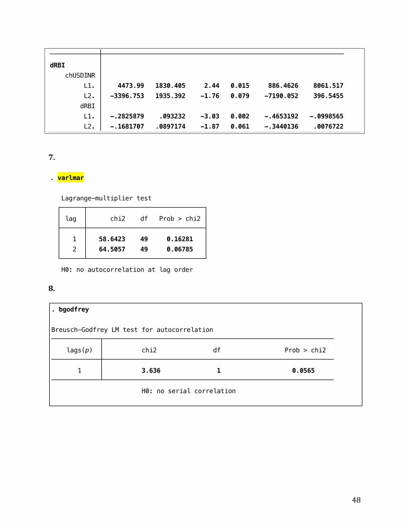
rendered moot by another one. All the lagged variables significantly correlated with their own

variable. This reeked of autocorrelation, and hence I performed a Lagrange Multiplier test of

serial correlation on the VAR. As feared, the statistic turned out to be significant at Lag 2, and I

had to begin again.

  34  

Had the VAR worked without errors, there would have been some interesting

relationships to analyze. The most interesting part about a VAR is that one can also observe the

relationship with lagged variables. The first effect that would have been interesting to identify

would be the relationship between the chTVPN and the chUSDINR variable. I would have

expected the coefficient to be positive and significant at the 5 % level. However, it would have

been more interesting to compare the coefficients on chTVPN and chAUCNPN with respect to

chUSDINR. Assuming chAUCNPN would have been significant, this comparison would have

revealed whether PNs had a greater effect on the USD/INR exchange rate than all other kinds of

FII flows. The lagged variable wouldn’t have revealed very much justifiable information because

of the one-month frequency.

The lagged relationship between Inflation and chUSDINR, as well as RBI and

chUSDINR would have been interesting to note. Assuming the relationships were significant, it

would have been useful to make sure that both the lagged regressors affected the regressand with

a positive coefficient.

  35  

Discussion

One of the limitations that this study had was the monthly frequency of the data.

Exchange rates tend to fluctuate every day. In fact, in Balance of Trade crises, countries like

India have devalued their currencies by over 20% in day. However, the fact that the data was

monthly, helped keep out some of the potential outliers from the daily data.

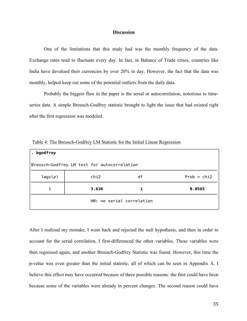
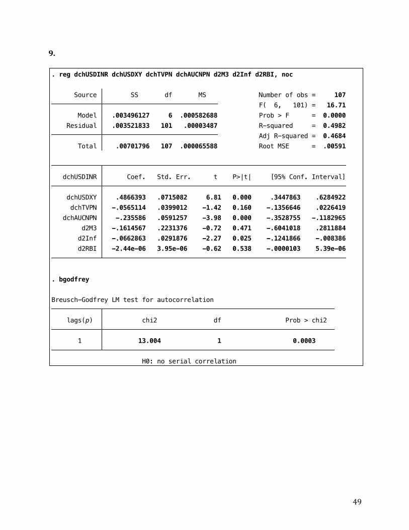
Probably the biggest flaw in the paper is the serial or autocorrelation, notorious to time-

series data. A simple Breusch-Godfrey statistic brought to light the issue that had existed right

after the first regression was modeled.

After I realized my mistake, I went back and rejected the null hypothesis, and then in order to

account for the serial correlation, I first-differenced the other variables. These variables were

then regressed again, and another Breusch-Godfrey Statistic was found. However, this time the

p-value was even greater than the initial statistic, all of which can be seen in Appendix A. I

believe this effect may have occurred because of three possible reasons: the first could have been

because some of the variables were already in percent changes. The second reason could have

. drop chTVPN[1]

H0: no serial correlation 1 3.636 1 0.0565 lags(p) chi2 df Prob > chi2 Breusch-Godfrey LM test for autocorrelation

. bgodfrey

Table 4: The Breusch-Godfrey LM Statistic for the Initial Linear Regression

  36  

been the lower bound on the TVPN and AUCNPN data caused a problem to differencing.

Another possible reason could have been the existence of multicollinearity between the

dependent variables. If it was strong enough, and in a specific direction, it could have thrown off

the standard errors by enough to make the test statistics insignificant.

  37  

Conclusion Although my VAR test failed to provide conclusive data on the experiment, from all the data and

information I have come across, PNs do not seem to have as big as an impact on the exchange

rate as the Indian Media makes it out to have. Initially there was definitely a big reason to be

concerned about PNs. Since the end-user was not known, there were many possible illegal uses

of the instrument, as mentioned in this thesis. Let’s look at the question of illegal money re-

entering the country. Although the government ends up loosing tax gains in the short term, it

repatriates money back into India in the long term. In any case the government of India has set

up charity schemes, through which people can begin to convert their illegal money into legal

money by paying a small fee.

From the many non-empirical analyses that I had to go through before I could write this

thesis, I would like to straw man two of the prominent volatility-related arguments that people

make against PNs. The first is the belief that when PN investors buy stocks, they do it as

speculators and not investors. This means they have an approximate investment horizon of less

than a year and bet on the market moving in a certain direction in that short horizon, instead of

expecting the company they invest in to do well in either case. I have two issues with that. For

the sake of argument, lets assume that all PN users are speculators, the speculation can only be

dangerous to the Rupee in the situation of a fear-driven, or irrational dumping of PNs. This is

still no reason to bar a financial instrument. In the worlds largest democracy (by population) I

pity the people who ascribe to cowardly politics instead of welcoming international competition.

The second problem I have with that claim is the fact that foreigners are stereotyped as

speculators. In some situations, firms may want to increase their risk exposure to India, or they

may want to hedge against their currency. Either way for the most part, these decisions are well

  38  

thought of investment strategies, in riskier countries with higher costs of Capital. The second and

probably biggest problem I have with PN critics is this belief of ‘Herd Mentality’ in foreign

investors. There has been some scientific work linking emotionally driven economic decision-

making being linked to information asymmetry, which many foreign investors in India

experience. Although there might be a financial basis for this potential sell-off in the future, it

does not warrant prejudice against the foreign investment community, or one of its vehicles in

India today. In spite of this, in a follow-up study, if it were found that the PNs do have an

adverse effect on the INR, it would be wise for the Indian government’s finance ministry to pass

laws better limiting the sale and trade of PNs.

  39  

Works Cited Bery, Suman, Bosworth, Barry P. and Panagariya, Arvind. India Policy Forum 2009/10. Volume 6: Editors' Summary. Brookings Institute, July 2009 Bhasin, Niti. Banking and financial markets in India, 1947 to 2007. New Century Publications, 2007. Budget Speech 1991-92. Shri Manmohan Singh, Minister of Finance. 24th July, 1991 http://www.indiabudget.nic.in/bspeech/bs199192.pdf Cerra, Valerie, and Sweta Chaman Saxena. "What caused the 1991 currency crisis in India?." IMF Staff Papers (2002): 395-425. Chandrasekhar, C. P. "Courting Risk: Policy Manoeuvres on FII Inflows." Economic and Political Weekly (2006): 92-95. Dhiman, Rahul. “Impact Of Foreign Institutional Investor On The Stock Market.” International Journal in Research of Finance and Marketing 2.4 (2012):32-46. Indian Securities Market Volume XIV 2011, www.nseindia.com/content/us/ismr_full2011.pdf  India,  1991  Country  Economic  Memorandum.  Vol.  1.  World  Bank,  1991   Lokeshwarri S.K. “The Fading Allure Of P-Notes.” Business Daily. January 28, 2011 Mankiw, Gregory N. "Principles of Macroeconomics, 5th." Ohio: South-Western Cengage Learning (2009). Mohan, TT Ram. "Stock market fall: Managing volatile flows." Economic and Political Weekly (2006): 2411-2413. Mohan, TT Ram. "Neither Dread Nor Encourage Them." Economic and Political Weekly (2006): 95-99. Position Paper on External Assistance Received by India, Government of India, Ministry of Finance, Department of Economic Affairs, New Delhi, March 2008 N., Nikhil Kumar, Implications of Hedge Funds on the Indian Capital Market (August 20, 2007) Rai, Kulwant, and N. R. Bhanumurthy. "Determinants of foreign institutional investment in India: The role of return, risk, and inflation." The Developing Economies 42.4 (2004): 479-493. Report of the Expert Group on Encouraging FII Flows and Checking the Vulnerability of Capital Markets to Speculative Flows, Government of India, Ministry of Finance, Department of Economic Affairs, New Delhi, November 2005 (also, Lahiri Committee)

  40  

Singh, Manmohan. Use of Participatory Notes in Indian Equity Markets and Recent Regulatory Changes. Vol. 7. International Monetary Fund, 2007. Securities And Exchange Board Of India (Foreign Institutional Investors) Regulations, 1995. www.sebi.gov.in/acts/act07a.html The Securities and Exchange Board of India Act (1992), www.sebi.gov.in/acts/act15ac.pdf Vasudevan, A. "A Note on Portfolio Flows into India." Economic and Political Weekly (2006): 90-92. “White Paper on Black Money.” Ministry of Finance, Department of Revenue, India. 2012. Wooldridge, Jeffrey M. Introductory econometrics: A modern approach. South-Western Pub, 2009.

  41  

Appendix A: STATA OUTPUT and SOME MANIPULATIONS    1.    . dfuller chUSDINR, lags(12) Augmented Dickey-Fuller test for unit root Number of obs = 95 ---------- Interpolated Dickey-Fuller --------- Test 1% Critical 5% Critical 10% Critical Statistic Value Value Value Z(t) -3.514 -3.517 -2.894 -2.582 MacKinnon approximate p-value for Z(t) = 0.0076 . dfuller chUSDXY, lags(12) Augmented Dickey-Fuller test for unit root Number of obs = 95 ---------- Interpolated Dickey-Fuller --------- Test 1% Critical 5% Critical 10% Critical Statistic Value Value Value Z(t) -4.596 -3.517 -2.894 -2.582 MacKinnon approximate p-value for Z(t) = 0.0001 . dfuller chTVPN, lags(12) Augmented Dickey-Fuller test for unit root Number of obs = 95 ---------- Interpolated Dickey-Fuller --------- Test 1% Critical 5% Critical 10% Critical Statistic Value Value Value Z(t) -2.703 -3.517 -2.894 -2.582 MacKinnon approximate p-value for Z(t) = 0.0736 . dfuller chAUCNPN, lags(12) Augmented Dickey-Fuller test for unit root Number of obs = 95

  42  

---------- Interpolated Dickey-Fuller --------- Test 1% Critical 5% Critical 10% Critical Statistic Value Value Value Z(t) -3.167 -3.517 -2.894 -2.582 MacKinnon approximate p-value for Z(t) = 0.0220 . dfuller chM3, lags(12) trend Augmented Dickey-Fuller test for unit root Number of obs = 95 ---------- Interpolated Dickey-Fuller --------- Test 1% Critical 5% Critical 10% Critical Statistic Value Value Value ------------------------------------------------------------------------------ Z(t) -1.990 -4.051 -3.455 -3.153 ------------------------------------------------------------------------------ MacKinnon approximate p-value for Z(t) = 0.6067 . dfuller RBI, lags(12) trend Augmented Dickey-Fuller test for unit root Number of obs = 95 ---------- Interpolated Dickey-Fuller --------- Test 1% Critical 5% Critical 10% Critical Statistic Value Value Value ------------------------------------------------------------------------------ Z(t) -2.666 -4.051 -3.455 -3.153 ------------------------------------------------------------------------------ MacKinnon approximate p-value for Z(t) = 0.2503 . dfuller Inflation, lags(12) trend Augmented Dickey-Fuller test for unit root Number of obs = 95 ---------- Interpolated Dickey-Fuller --------- Test 1% Critical 5% Critical 10% Critical Statistic Value Value Value ------------------------------------------------------------------------------ Z(t) -2.360 -4.051 -3.455 -3.153 ------------------------------------------------------------------------------ MacKinnon approximate p-value for Z(t) = 0.4013

  43  

. dfuller dchM3, lags(12) Augmented Dickey-Fuller test for unit root Number of obs = 94 ---------- Interpolated Dickey-Fuller --------- Test 1% Critical 5% Critical 10% Critical Statistic Value Value Value ------------------------------------------------------------------------------ Z(t) -6.988 -3.518 -2.895 -2.582 ------------------------------------------------------------------------------ MacKinnon approximate p-value for Z(t) = 0.0000 . dfuller dRBI, lags(12) Augmented Dickey-Fuller test for unit root Number of obs = 94 ---------- Interpolated Dickey-Fuller --------- Test 1% Critical 5% Critical 10% Critical Statistic Value Value Value ------------------------------------------------------------------------------ Z(t) -4.480 -3.518 -2.895 -2.582 ------------------------------------------------------------------------------ MacKinnon approximate p-value for Z(t) = 0.0002 . dfuller dInflation, lags(12) Augmented Dickey-Fuller test for unit root Number of obs = 94 ---------- Interpolated Dickey-Fuller --------- Test 1% Critical 5% Critical 10% Critical Statistic Value Value Value ------------------------------------------------------------------------------ Z(t) -5.852 -3.518 -2.895 -2.582 ------------------------------------------------------------------------------ MacKinnon approximate p-value for Z(t) = 0.0000        

  44  

2.    

   .  predict  res1,  r  (3  missing  values  generated)    .                                      

_cons .0011491 .0004691 2.45 0.016 .0002185 .0020796 dRBI 3.98e-07 4.93e-06 0.08 0.936 -9.39e-06 .0000102 dInflation -.0549006 .0388463 -1.41 0.161 -.1319612 .0221599 dchM3 -.1968207 .3013988 -0.65 0.515 -.7947148 .4010733 chAUCNPN -.2260905 .0698298 -3.24 0.002 -.364614 -.087567 chTVPN -.1123166 .0447407 -2.51 0.014 -.2010701 -.0235631 chUSDXY .4747286 .0832284 5.70 0.000 .3096259 .6398313 chUSDINR Coef. Std. Err. t P>|t| [95% Conf. Interval]

Total .004352597 107 .000040678 Root MSE = .0047 Adj R-squared = 0.4559 Residual .002235628 101 .000022135 R-squared = 0.4864 Model .002116969 6 .000352828 Prob > F = 0.0000 F( 6, 101) = 15.94 Source SS df MS Number of obs = 108

. reg chUSDINR chUSDXY chTVPN chAUCNPN dchM3 dInflation dRBI

  45  

3.`  graph  twoway  line  res1  Month    

   4.      

       

.

Exogenous: chUSDXY chTVPN chAUCNPN dchM3 dRBI dInflation _cons Endogenous: chUSDINR 4 418.586 2.5433 1 0.111 .000023 -7.83819 -7.72487 -7.55849 3 417.314 .16348 1 0.686 .000023 -7.83296 -7.72995 -7.5787 2 417.232 1.6845 1 0.194 .000023 -7.85062 -7.75791 -7.62178 1 416.39 .45564 1 0.500 .000023 -7.85366 -7.77125 -7.65024 0 416.162 .000022* -7.86851* -7.7964* -7.69052* lag LL LR df p FPE AIC HQIC SBIC Sample: Jan 2004 - Aug 2012 Number of obs = 104 Selection-order criteria

. varsoc chUSDINR, exog(chUSDXY chTVPN chAUCNPN dchM3 dRBI dInflation)

  46  

5.      

       6.    

 

7 56 1805.3922 0.36180 6 55 1781.8147 0.44548 47.1551 3.76 5 52 1750.8581 0.56070 109.0683 15.41 4 47 1707.673 0.63082 195.4384 29.68 3 40 1655.3586 0.66074 300.0672 47.21 2 31 1598.607 0.73330 413.5705 68.52 1 20 1529.2217 0.80987 552.3411 94.15 0 7 1442.068 . 726.6484 124.24 rank parms LL eigenvalue statistic valuemaximum trace critical 5% Sample: Dec 2003 - Aug 2012 Lags = 1Trend: constant Number of obs = 105 Johansen tests for cointegration

. vecrank chUSDINR chUSDXY chTVPN chAUCNPN dchM3 dRBI dInflation, lag(1)

_cons .0001856 .0006273 0.30 0.767 -.0010438 .001415 L2. -6.84e-06 6.43e-06 -1.06 0.287 -.0000195 5.77e-06 L1. -1.52e-06 6.69e-06 -0.23 0.820 -.0000146 .0000116 dRBI L2. .0868708 .0589421 1.47 0.141 -.0286535 .2023951 L1. .1772865 .0546875 3.24 0.001 .0701011 .284472 dInflation L2. .2766459 .4274654 0.65 0.518 -.5611709 1.114463 L1. .6210479 .4468315 1.39 0.165 -.2547257 1.496821 dchM3 L2. .119262 .0911398 1.31 0.191 -.0593687 .2978928 L1. .0763586 .0938955 0.81 0.416 -.1076733 .2603904 chAUCNPN L2. -.074831 .0587907 -1.27 0.203 -.1900586 .0403966 L1. -.0584354 .061371 -0.95 0.341 -.1787204 .0618495 chTVPN L2. .1658357 .1191602 1.39 0.164 -.0677141 .3993855 L1. -.0672624 .1232086 -0.55 0.585 -.3087469 .1742221 chUSDXY L2. -.1783786 .1387755 -1.29 0.199 -.4503737 .0936165 L1. .2460982 .1312475 1.88 0.061 -.0111422 .5033386 chUSDINR chUSDINR Coef. Std. Err. z P>|z| [95% Conf. Interval]

dRBI 15 86.062 0.2591 37.06522 0.0007dInflation 15 .010497 0.3389 54.34967 0.0000dchM3 15 .001276 0.4019 71.22096 0.0000chAUCNPN 15 .007423 0.1434 17.74913 0.2184chTVPN 15 .010849 0.2323 32.07855 0.0039chUSDXY 15 .006102 0.0680 7.730514 0.9029chUSDINR 15 .006171 0.2023 26.88937 0.0199 Equation Parms RMSE R-sq chi2 P>chi2

Det(Sigma_ml) = 1.36e-24 SBIC = -30.47234FPE = 9.97e-24 HQIC = -32.04133Log likelihood = 1859.864 AIC = -33.11065Sample: Dec 2003 - Sep 2012 No. of obs = 106

Vector autoregression

. var chUSDINR chUSDXY chTVPN chAUCNPN dchM3 dInflation dRBI, lag(1 2)

  47  

 

 

 

   

 

 

 

 

L2. -.1783786 .1387755 -1.29 0.199 -.4503737 .0936165 L1. .2460982 .1312475 1.88 0.061 -.0111422 .5033386 chUSDINR chUSDINR Coef. Std. Err. z P>|z| [95% Conf. Interval]

L2. .0868708 .0589421 1.47 0.141 -.0286535 .2023951 L1. .1772865 .0546875 3.24 0.001 .0701011 .284472 dInflation

chUSDINR chUSDXY

L2. -.052197 .0581317 -0.90 0.369 -.1661331 .0617391 L1. -.1132866 .0606831 -1.87 0.062 -.2322233 .00565 chTVPN

L2. -.0200228 .2439804 -0.08 0.935 -.4982156 .45817 L1. -.7192643 .2307454 -3.12 0.002 -1.171517 -.2670116 chUSDINR chTVPN

_cons .0019712 .0011028 1.79 0.074 -.0001902 .0041326

L1. -.175022 .1578714 -1.11 0.268 -.4844441 .1344002 chUSDINR chAUCNPN

L2. .3280637 .1669265 1.97 0.049 .0008939 .6552336

L1. -.0353152 .1482018 -0.24 0.812 -.3257854 .2551549 chUSDXY

L2. -.2620619 .1433322 -1.83 0.067 -.5429878 .0188639

L2. .0964713 .0707165 1.36 0.173 -.0421305 .2350731 L1. .1743466 .0738202 2.36 0.018 .0296617 .3190316 chTVPN

_cons .0016634 .0007545 2.20 0.027 .0001846 .0031422

chUSDINR dchM3

L2. -.0293989 .0121867 -2.41 0.016 -.0532844 -.0055133 L1. -.0382377 .0113071 -3.38 0.001 -.0603992 -.0160763 dInflation L2. -.260749 .088382 -2.95 0.003 -.4339745 -.0875236 L1. -.6366976 .092386 -6.89 0.000 -.8177709 -.4556243 dchM3

chUSDINR dInflation

L2. -.2799954 .1002627 -2.79 0.005 -.4765067 -.083484 L1. -.5587198 .0930255 -6.01 0.000 -.7410464 -.3763932 dInflation

  48  

 

   7.  

   8.    

                 

L2. -3396.753 1935.392 -1.76 0.079 -7190.052 396.5455 L1. 4473.99 1830.405 2.44 0.015 886.4626 8061.517 chUSDINR dRBI

L2. -.1681707 .0897174 -1.87 0.061 -.3440136 .0076722 L1. -.2825879 .093232 -3.03 0.002 -.4653192 -.0998565 dRBI

H0: no autocorrelation at lag order 2 64.5057 49 0.06785 1 58.6423 49 0.16281 lag chi2 df Prob > chi2 Lagrange-multiplier test

. varlmar

. drop chTVPN[1]

H0: no serial correlation 1 3.636 1 0.0565 lags(p) chi2 df Prob > chi2 Breusch-Godfrey LM test for autocorrelation

. bgodfrey

  49  

9.    

  H0: no serial correlation 1 13.004 1 0.0003 lags(p) chi2 df Prob > chi2 Breusch-Godfrey LM test for autocorrelation

. bgodfrey

d2RBI -2.44e-06 3.95e-06 -0.62 0.538 -.0000103 5.39e-06 d2Inf -.0662863 .0291876 -2.27 0.025 -.1241866 -.008386 d2M3 -.1614567 .2231376 -0.72 0.471 -.6041018 .2811884 dchAUCNPN -.235586 .0591257 -3.98 0.000 -.3528755 -.1182965 dchTVPN -.0565114 .0399012 -1.42 0.160 -.1356646 .0226419 dchUSDXY .4866393 .0715082 6.81 0.000 .3447863 .6284922 dchUSDINR Coef. Std. Err. t P>|t| [95% Conf. Interval]

Total .00701796 107 .000065588 Root MSE = .00591 Adj R-squared = 0.4684 Residual .003521833 101 .00003487 R-squared = 0.4982 Model .003496127 6 .000582688 Prob > F = 0.0000 F( 6, 101) = 16.71 Source SS df MS Number of obs = 107

. reg dchUSDINR dchUSDXY dchTVPN dchAUCNPN d2M3 d2Inf d2RBI, noc