The Impact of Regulation on Mortgage Risk: Evidence from India John Y. Campbell, Tarun Ramadorai, and Benjamin Ranish y This version: September 2014 First draft: September 2012 Abstract We employ loan-level data on over a million loans disbursed in India between 1995 and 2010 to understand how fast-changing regulation impacted mortgage lending and risk. Our paper uses changes in regulatory treatment discontinuities associated with loan size and leverage to detect regulation-induced loan delinquencies. We also nd that an acceleration in the classication of assets as non-performing resulted in substantially lower delinquency probabilities and losses given delinquency. We gratefully acknowledge an Indian mortgage provider for providing us with the data, and many em- ployees of the Indian mortgage provider, Santosh Anagol, Amit Bubna, Jishnu Das, Jennifer Huang, Ajay Shah, S. Sridhar, Usha Thorat, R. V. Verma, Vikrant Vig, Alan Auerbach (the editor) and two anonymous referees for useful comments and discussions. We thank seminar participants at the Econometric Soci- ety/European Economics Association Malaga Conference, the NBER Household Finance Summer Institute, IIM Bangalore, the World Bank, the Oxford-Man Institute of Quantitative Finance, Sad Business School, the HKUST Household Finance Symposium, the NUS-IRES Real Estate Symposium, the NHB-CAFRAL Conference, and the NIPFP-DEA Conference on International Capital Flows for comments, the Interna- tional Growth Centre and the Sloan Foundation for nancial support, and Vimal Balasubramaniam, Gaurav Kankanhalli, and Kevin Wang for able research assistance. An earlier version of this paper was circulated under the title How Do Regulators Inuence Mortgage Risks? Evidence from an Emerging Market. y Campbell: Department of Economics, Littauer Center, Harvard University, Cambridge MA 02138, USA, and NBER. Email [email protected]. Ramadorai: Sad Business School, Oxford-Man Institute of Quantitative Finance, University of Oxford, Park End Street, Oxford OX1 1HP, UK, and CEPR. Email [email protected]. Ranish: Board of Governors of the Federal Reserve System, 1850 K Street NW, Mailstop 1800, Washington, DC 20006. Email [email protected]. The views in this paper are solely the responsibility of the authors and should not be interpreted as those of the Board of Governors of the Federal Reserve System, or of other members of their sta/.
Transcript
The Impact of Regulation on Mortgage Risk:
Evidence from India∗
John Y. Campbell, Tarun Ramadorai, and Benjamin Ranish†
This version: September 2014
First draft: September 2012
Abstract
We employ loan-level data on over a million loans disbursed in India between 1995and 2010 to understand how fast-changing regulation impacted mortgage lending andrisk. Our paper uses changes in regulatory treatment discontinuities associated withloan size and leverage to detect regulation-induced loan delinquencies. We also find thatan acceleration in the classification of assets as non-performing resulted in substantiallylower delinquency probabilities and losses given delinquency.
∗We gratefully acknowledge an Indian mortgage provider for providing us with the data, and many em-ployees of the Indian mortgage provider, Santosh Anagol, Amit Bubna, Jishnu Das, Jennifer Huang, AjayShah, S. Sridhar, Usha Thorat, R. V. Verma, Vikrant Vig, Alan Auerbach (the editor) and two anonymousreferees for useful comments and discussions. We thank seminar participants at the Econometric Soci-ety/European Economics Association Malaga Conference, the NBER Household Finance Summer Institute,IIM Bangalore, the World Bank, the Oxford-Man Institute of Quantitative Finance, Saïd Business School,the HKUST Household Finance Symposium, the NUS-IRES Real Estate Symposium, the NHB-CAFRALConference, and the NIPFP-DEA Conference on International Capital Flows for comments, the Interna-tional Growth Centre and the Sloan Foundation for financial support, and Vimal Balasubramaniam, GauravKankanhalli, and Kevin Wang for able research assistance. An earlier version of this paper was circulatedunder the title “How Do Regulators Influence Mortgage Risks? Evidence from an Emerging Market.”†Campbell: Department of Economics, Littauer Center, Harvard University, Cambridge MA 02138, USA,
and NBER. Email [email protected]. Ramadorai: Saïd Business School, Oxford-Man Instituteof Quantitative Finance, University of Oxford, Park End Street, Oxford OX1 1HP, UK, and CEPR. [email protected]. Ranish: Board of Governors of the Federal Reserve System, 1850 K StreetNW, Mailstop 1800, Washington, DC 20006. Email [email protected]. The views in this paper are solelythe responsibility of the authors and should not be interpreted as those of the Board of Governors of theFederal Reserve System, or of other members of their staff.
1 Introduction
How does mortgage regulation influence the structure and performance of housing finance?
This paper answers the question with administrative data on over 1.2 million loans originated
by an Indian mortgage provider. We relate loan pricing and delinquency rates to the
changing details of Indian mortgage regulation.
One way to understand how government involvement affects mortgage markets is to col-
lect evidence from cross-country data, as in International Monetary Fund (2011). This ap-
proach is complicated by the diffi cult to measure and potentially unobservable factors which
may affect household mortgage choice across countries. For example, historical experiences
with interest rate and inflation volatility can have long-lasting effects because consumers can
be slow to adopt new financial instruments (Campbell 2013).
A promising alternative is to trace the effects of changing mortgage regulation over time
within a single country, but this approach is diffi cult to implement in developed countries, as
they tend to have fairly stable systems of financial regulation. This creates few opportunities
to observe the effects of sharp regulatory changes. Slow changes, such as those that occurred
in the US during the early and mid-2000s, may well be important but it is hard to show
this convincingly. For this reason academic writers and public policy commentators have
reached little consensus on the degree to which regulation, rather than other factors, caused
the US mortgage credit boom.1
Mortgages are rapidly becoming important financial instruments in emerging markets.
Here, financial regulation is at least as intrusive and much less stable. In addition, long-
lasting historical influences are likely to be less important in emerging markets because their
rapid growth and financial evolution reduce consumer inertia. For this reason, emerging
markets are ideal laboratories in which to examine the effects of mortgage regulation.
Our study focuses on the mortgage market in India. The provision of housing finance in
1A range of views can be found in Acharya, Richardson, van Nieuwerburgh, and White (2011), Baily(2011), Ellis (2008), International Monetary Fund (2011), and US Treasury and Department of Housingand Urban Development (2011), among other sources. Dahl, Evanoff, and Spivey (2000), Kroszner (2008),Avery and Brevoort (2011), and Agarwal, Benmelech, Bergman, and Seru (2012) debate the importance ofthe Community Reinvestment Act (CRA) in encouraging risky lending to lower-income borrowers.
1
India is evolving particularly rapidly (Tiwari and Debata 2008, Verma 2012). Regulatory
norms have changed frequently, albeit with a continuing emphasis on funding housing for low-
income households. The country has been studied extensively by the economics profession,
mainly to analyze issues of poverty and development (see for example Besley and Burgess
2000 and Banerjee, Cole, Duflo, and Linden 2007), or the impact of the Byzantine system
of laws and regulations on industrial organization and firm output (see for example Aghion,
Burgess, Redding, and Zilibotti 2008 and von Lilienfeld-Toal, Mookherjee, and Visaria 2012).
India underwent an economic liberalization in the early 1990s and subsequently experienced
rapid economic growth that accelerated further in the 2000s. During this time the financial
sector has become much larger and more sophisticated, but remains highly regulated, with a
significantly nationalized banking sector. Recently, authors such as Anagol and Kim (2012)
have begun to study Indian financial regulation and its impacts on fast-changing Indian
capital markets.
Rich microeconomic data are necessary to convincingly answer questions about loan
structure and performance, and we are fortunate to have access to loan-level administrative
data from an Indian mortgage provider.2 While our study is limited by its focus on data from
a single mortgage provider, the large number of loans that we analyze, the broad geographical
distribution of the loans, and the quarter-century over which the data are available provide
some confidence in the broader validity of our results. In addition we note that the Indian
mortgage lending market was highly concentrated early in our sample period, which implies
that data from a single provider can represent a meaningful fraction of total Indian mortgage
lending.3
Our ability to use micro-data is particularly important for our study, because pure time-
series variation in mortgage risk, even if correlated with changing regulation, may also be
2Some recent mortgage studies using US microeconomic data include Adelino, Gerardi, and Willen (2013),Agarwal, Amromin, Ben-David, Chomsisengphet, and Evanoff (2011), Amromin, Huang, Sialm, and Zhong(2011), Bhutta, Dokko, and Shan (2010), Demyanyk and van Hemert (2011), Foote, Gerardi, Goette, andWillen (2010), Johnson and Li (2011), Keys, Mukherjee, Seru, and Vig (2010), Melzer (2011), Mian and Sufi(2009), and Piskorski, Seru, and Vig (2011).
3More recently, however, there has been increasing competition between mortgage lenders, a fact whichmay have contributed to rapidly increasing house prices since 2002.
2
explained by the changing state of the macroeconomy. Instead, our difference-in-difference
approach searches for effects of regulatory changes on loan delinquencies, by focusing on
changes in regulatory treatment discontinuities in loan characteristics such as loan size and
loan-to-value (LTV) ratios.
Our approach yields three main findings on the relation between regulation and mortgage
risk. First, throughout the period of study, small and micro loans are particularly favoured
by the Indian regulatory environment. We show that implicit subsidies to smaller loans
qualifying as “priority sector lending ”(PSL) show up as discontinuities in both the volume
of lending and delinquency rates at the qualifying threshold– with loan delinquency rates
being substantially higher just under the qualifying threshold than just above. These
discontinuities appear even though we control for the initial interest rates charged by the
mortgage lender, implying that the lender is willing to accept a higher delinquency rate for
a similar loan interest rate (or equivalently, is willing to charge a lower interest rate for a
comparable delinquency rate) when a loan is PSL-qualifying. The nominal PSL-qualifying
loan size threshold was reset only four times during our quarter-century sample, despite
rapidly rising nominal home prices over the period. We show that the discontinuities in loan
delinquency rates around the PSL thresholds are larger just prior to threshold resets– times
at which the PSL requirement should bind most tightly.
Our second finding concerns the impact of variation in mortgage lender capital require-
ments, which in India takes the form of changes in risk weights on mortgages with different
LTV ratios. Over the period that we study, the risk weights for mortgages disbursed at LTV
ratios of 75% or below have varied from between 50% and 100% of the risk weights for loans
with higher LTV ratios. We find that when risk weights on mortgages disbursed at LTV
ratios at and just under 75% are relatively lower, the subsequent delinquency rates on these
mortgages are relatively higher, after accounting for interest rates at loan issuance. Fur-
thermore, the size of this discontinuity in delinquency rates tracks the size of the risk weight
advantage given to relatively lower-leverage loans. Once again this implies that the lender
is willing to accept a higher delinquency rate for a similar loan interest rate (or equivalently,
is willing to charge a lower interest rate for a comparable delinquency rate) when a mortgage
3
loan receives a more favorable risk weight. These findings confirm predictions that changes
in risk weights do impact bank lending activity, and ultimately loan delinquencies (see, for
example, Calem and Follain 2007, and Balasubramanyan and Jacques 2011).
Our third finding relates to a regulatory reclassification of “non-performing assets”(NPAs)
from loans that are 180 days delinquent on contracted payments to those that are only 90
days delinquent on payments. Since capital provisioning requirements against delinquen-
cies are tied to this classification, this change incentivizes the mortgage provider to monitor
loans earlier, and potentially to intensify loan screening. We obtain a random subsample
of loans from the lender for which we are given a complete time series of payment histories,
and we show that this regulatory reclassification appears to result in greater effort expended
on monitoring delinquencies approaching the 90-day mark. Specifically, we find that the
lender’s likelihood of experiencing both short-term (90-day) delinquencies and longer-term
defaults falls substantially. We find that the impact of this change on long-term defaults is
even larger than that arising from a 2002 legal change in the ability of mortgage providers
to more easily repossess or restructure non-performing assets. Finally, we also find evidence
that there is more rigorous screening of loan quality prior to issuance following this redef-
inition of NPAs; mortgage cohorts disbursed shortly after the change experience fewer and
less costly delinquencies than those disbursed shortly before.
This evidence from India contributes to the debate on whether incentives for lending to
lower-income borrowers in other countries, such as those created by the U.S. Community
Reinvestment Act (CRA), have affected loan delinquencies (see, for example, Canner and
Passmore 1997, Dahl, Evanoff, and Spivey 2000, Kroszner 2008, Avery and Brevoort, 2011,
and Agarwal, Benmelech, Bergman, and Seru 2012).4 Our results also relate to evidence
that mortgage credit expansion in the U.S., particularly in sub-prime zipcodes, contributed
to the rise in mortgage delinquencies and the broader economic downturn after 2007 (Mian
and Sufi2009, Demyanyk and van Hemert 2011). Finally, our results are consistent with the
4Regulatory loan size thresholds have also been studied in other contexts. For example, DeFusco andPaciorek (2014) and Adelino, Schoar, and Severino (2014) use the conforming loan limit in the U.S. tomeasure interest rate elasticity, and the impact of the implied lending subsidies on home prices, respectively.
4
finding of Keys, Mukherjee, Seru, and Vig (2011) that U.S. regulatory norms have affected
mortgage screening.
It is worth mentioning two caveats about our findings. First, our results do not allow us to
make claims about the potential welfare improvements associated with changes in regulatory
policy. There may be substantial public benefits associated with programs intended to
expand credit to lower-income and potentially less creditworthy borrowers, and we do not
measure these benefits in our paper.
Nevertheless, we believe that paying attention to the details of policy design may yield
significant benefits. Our results suggest that the current form of the PSL policy may be
sub-optimal, with substantial increases in delinquencies in periods when nominal thresholds
remain constant while house prices are rising, and corresponding reductions in these delin-
quencies when nominal thresholds are (infrequently) adjusted. A better-designed policy
might simply index the PSL-qualifying nominal threshold to a commonly available house
price index to avoid this “lumpy adjustment”of delinquency rates. This would be helpful to
allow lenders to better manage their balance sheets, and might reduce the social costs that
can arise from spikes in default rates (Campbell, Giglio, and Pathak 2011).
Second, while we do measure significant benefits from early action on potentially delin-
quent loans, we are unable to measure the costs of improving screening and monitoring,
which include both direct costs to lenders and the impact of screening on access to credit.
While this makes it diffi cult for us to assess the net welfare impact of responding more
quickly to potential delinquencies, more work in this area might be worthwhile given the
large benefits that we identify.
The organization of the paper is as follows. Section 2 describes the Indian macroeco-
nomic environment and the Indian system of mortgage regulation during the quarter century
since 1985, together with the mortgage data we employ. Further details of Indian mortgage
regulation are provided in an online regulatory appendix (Campbell, Ramadorai, and Bala-
subramaniam 2014). Section 3 introduces our model of mortgage delinquencies, which we
use to explore the effects of regulation– specifically, quotas on priority sector lending and risk
weights on lower loan-value mortgages– on the relative delinquency rates of different types
5
of loans. Section 4 discusses the change in the regulatory classification of non-performing
assets in 2004 and its consequences for observed delinquency and repayment patterns. Sec-
tion 5 concludes. Additional empirical evidence on the Indian mortgage market is reported
in an online empirical appendix (Campbell, Ramadorai, and Ranish 2014).
2 The Macroeconomic and Regulatory Environment
2.1 Macroeconomic Trends
Table 1 summarizes the history of several important Indian macroeconomic variables over
the period 1985—2010, including annual real GDP growth, CPI inflation, and government
bond yields. Regulatory and macroeconomic reform in the early 1990s was followed by
growth in the 4-8% range until the early 2000s, when growth accelerated above 8%, briefly
slowed again only by the global financial crisis in 2008. Meanwhile inflation was high and
volatile during the 1990s, with volatility particularly elevated around the reform period and
in 1998—99. A period of more stable inflation followed in the 2000s, but inflation accelerated
at the very end of our sample period.
Indian government bond yields over the same period were correspondingly volatile. The
1-year yield declined from double-digit levels in the mid-1990s, with a brief reversal in the
late 1990s. After a low of about 5% in the early 2000s, the 1-year yield spiked up to
almost 8% in 2008, again related to concerns about inflation. The 10-year yield moved
more smoothly but also declined substantially from the mid-1990s until the early 2000s.
Figure 1 plots real house price indexes, both for India as a whole and for five broad
regions. The real rate of house price appreciation for the country as a whole is also reported
in Table 1. We compute these indexes using the mortgage provider’s own property cost
data, but data from the National Housing Bank (NHB), which are available for only part
of the sample period, show similar patterns. Indian house prices were relatively stable until
the early 2000s and then began to increase rapidly, particularly in the south of the country.
The southern index peaked in 2008 while some other regions peaked in 2009. Thus India
6
took part in the worldwide housing boom despite many differences in other aspects of its
macroeconomic performance.
These house price movements are important for our study because they interact with
government policies favoring smaller loans. As house prices increase and the priority sector
qualifying threshold remains constant, fewer loans naturally qualify for lenders’ priority
sector lending quotas, creating time variation in the tightness of regulatory constraints on
mortgage lending.
2.2 The Regulatory Environment
Mortgages in India are originated by two types of financial institutions, banks and housing
finance companies (HFCs). Banks are regulated by the Reserve Bank of India (RBI), while
housing finance companies are regulated by the National Housing Bank (NHB), but most
regulations apply in fairly similar form to the two types of institution. This fact is important
for our study, as we are unable to publicly identify whether our mortgage provider is a bank
or an HFC.
Figure 2 summarizes the details of mortgage regulation in India. The top half of the
figure shows regulations that applied to banks, and the bottom half shows regulations that
applied to HFCs. The regulations that remained constant throughout the period are listed
in Roman font, whereas the ones that changed over the period are in italic font. In light
of the significant changes that took place from 2001 to 2002, we separate the timeline into
the “first period,” i.e. prior to March 2001, and the “second period”which extends from
April 2001 until the end of 2010. In the middle of the figure, we summarize subsidy schemes
for micro-lending with the bars accompanying these schemes identifying their start and end
dates relative to the timeline.
Regulations can be divided into two types: those that restrict the funding of mortgage
lending in general, and those that incentivize lending to certain borrowers. Until 2001,
mortgage funding was regulated in a fairly traditional manner, using leverage restrictions on
banks and HFCs, and interest-rate ceilings on deposit-taking HFCs. From 2002 onwards,
7
these measures were augmented by capital requirements against risk-weighted assets follow-
ing the internationally standard Basel II framework. The RBI and NHB distinguished small
and very large loans, and loan-to-value (LTV) ratios above and below 75%, and set different
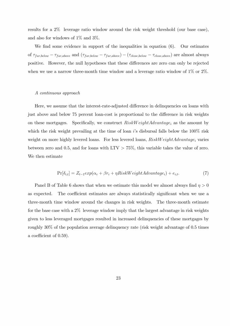
risk weights for these different categories. Figure 3 shows the difference in risk weights on
more and less leveraged loans originated by banks (dotted line) and HFCs (dashed line) over
time. The regulatory preference for less leveraged loans was greatest during the period 2002
to 2004.
It is important to note here that a majority of Indian mortgage providers chose to in-
terpret these LTV regulations as applying to loan-to-cost (LTC) ratios, where transactions
costs such as stamp duty land tax and registration and documentation charges were added
into the property value at the time of purchase. This practice was so widely prevalent that
the RBI issued a circular in February 2012, fourteen months following the end of our sample
period, to discourage this practice (see the online regulatory appendix for details). We are
provided with LTC data, and we use the terms LTC and LTV interchangeably in our analysis
below.
Another noteworthy change in the regulatory environment is highlighted on the timeline
in Figure 2, and occurred on March 31, 2004 for banks, and one year later, i.e., March 31,
2005 for HFCs. At this time the RBI reclassified an asset as a “non-performing asset”
(or NPA) if payments (on interest or principal) remained overdue for a period of ninety
days or more, from the previous 180 day period allowed before assets were so classified. One
important implication of the classification of an asset as an NPA is that it incurs provisioning
requirements, meaning that the capital available to a mortgage lender holding such an asset
reduces as the lender is required to hold precautionary capital to cover expected losses.
Related to this NPA reclassification, an important law which came into force somewhat
earlier (in July 2002), was the Securitization and Reconstruction of Financial Assets and
Enforcement of Security Interest (SARFAESI) Act. This law enabled the easier recovery
of NPAs via securitization, reconstruction, or direct repossession, bypassing the need for
secured creditors to seek permission from debt recovery tribunals (see von Lilienfeld-Toal,
Mookherjee, and Visaria 2012 on the impacts of the establishment of these tribunals in 1993,
8
and Vig 2013 on the impacts of SARFAESI on Indian firms). In our analysis, we separately
evaluate the impact of these two changes, namely the reclassification of NPAs in 2004, and
the introduction of SARFAESI in 2002, on delinquency costs experienced by the mortgage
provider.
Lending to small borrowers is an important political goal in India. Banks are subject to
a quantity target for priority sector lending (PSL), which includes loans to agriculture, small
interest to us– mortgages for low-cost housing. The PSL target is 40% of net bank credit
for domestic banks (32% for foreign banks), and there is a severe financial penalty for failure
to meet the target, namely, compulsory lending to rural agriculture at a haircut to the repo
rate. This regulation does not directly apply to HFCs, but bank lending to an HFC qualifies
for the PSL target to the extent that the HFC makes mortgage loans that qualify, i.e., are
below the nominal PSL threshold shown in Figure 3. The overall effect of the PSL system
is to provide an incentive, directly for banks, and indirectly for HFCs, to originate small
mortgages that (typically) finance low-cost housing purchases.
In addition to the PSL system, other schemes have been introduced at various times to
subsidize new or refinanced micro-lending– i.e., loans of sizes well below the PSL-qualifying
threshold. The mid-section of Figure 2 shows the various schemes that were in place during
our sample period to incentivize mortgage lending in very small loan sizes. These schemes
apply to both banks and HFCs. Most recently, interest rate subventions have been put
in place for the first year of repayments on small loans, payments that are passed through
to the borrower in the form of a reduced interest rate, for housing loans up to a maximum
size. Special subsidy and refinancing schemes in place for very small rural loans (the Golden
Jubilee Rural Housing Finance Scheme or GJRHFS, and the Indira Awaas Yojana) and for
borrowers qualifying for affi rmative action (the Differential Rate of Interest scheme) are also
shown in the figure, over the period for which they applied. Taken together, these schemes
increase the subsidy for tiny loans over and above the standard subsidy to PSL-qualifying
loans.
The online regulatory appendix, Campbell, Ramadorai, and Balasubramaniam (2014),
9
provides further details about the regulatory system, and serves as a comprehensive guide
to Indian mortgage regulation over the period of our study.
2.3 Evolution of the Mortgage Market
Both macroeconomic and regulatory forces have contributed to rapid change in the Indian
mortgage market. Table 2 illustrates the changes in three relevant characteristics of mort-
gages issued by our lender: the shares of variable-rate mortgages, and two categories of loans
relatively favored by the regulatory environment, namely, small PSL-qualifying loans, and
mortgages with loan-cost ratios at or below 75%.
The first two columns of Table 2 report the variable-rate share in the number and value
of mortgages disbursed. There has been a dramatic shift in the Indian mortgage system
away from fixed-rate and towards variable-rate mortgages, with one brief interruption in
2004. Our lender issued very few fixed-rate mortgages after 2007. During the period of
transition through 2002, variable-rate mortgages had somewhat larger principal amounts on
average than fixed-rate mortgages, as shown by their higher share of value in the second
column of the table.
The next two columns of the table report the share of mortgages that are below the
PSL threshold, separately for variable-rate and fixed-rate mortgages. The share below the
PSL threshold peaks in 2000 for both fixed- and variable-rate mortgages, and then declines
precipitously during the 2000s. The PSL-qualifying share is somewhat higher for fixed-rate
mortgages, reflecting their smaller average size.
The final two columns of the table report the share of mortgages with loan-cost ratios at
or below 75%, again separately for variable-rate and fixed-rate mortgages. This share trends
downwards, particularly rapidly in the early 2000s (for variable-rate mortgages) and the late
1990s (for fixed-rate mortgages). Both these trends are driven in part by the increase in
house prices during the mid-1990s and mid-2000s, shown earlier in Table 1 and Figure 1.
Table 3 presents more details on cohorts of loans issued in each year. Panel A reports
equally weighted cross-sectional cohort means of mortgage terms and delinquency rates.
10
Initial interest rates on variable-rate and fixed-rate mortgages track one another very closely
until 2002, and are both close to the Indian prime rate shown in Table 1, despite some
variation in the spread between long-term and short-term government yields. In the period
2003—06, the variable mortgage rate is well above the fixed rate and has an unusually high
spread over the 1-year bond yield, a feature shared with the Indian prime rate. This period
has a generally high market share for variable mortgages, but does include an episode in 2004
when our mortgage lender shifted back towards fixed mortgage issuance. Variable mortgage
rates decline after 2008, a period where our lender made few fixed-rate mortgages.
Panel A also summarizes cohort means of loan maturity, loan-cost ratios, and loan-
income ratios. The previously discussed increase in loan-cost ratios is visible here too, but
loan maturity and loan-income ratios are much more stable. This pattern contrasts with
mortgage trends during the 2000s in the US, where loan-income ratios increased more rapidly
than loan-value ratios (Campbell and Cocco 2014).
The right-hand columns report the cohort 90-day delinquency rate, the annual probability
that an outstanding and not-yet-delinquent loan experiences a 90-day delinquency, calculated
separately for each disbursal-year cohort and calendar year, and then averaged over calendar
years for each cohort. The early 2000s appear unusual in the sense that the cohort default
rate for mortgages disbursed in these years is high relative to the other cohorts in the sample
period, despite loan characteristics such as loan-cost and loan-income ratios not changing
much on average. The 2004 fixed-rate cohort, however, appears to have a significantly lower
default rate.
The top plot of Figure 4 summarizes Indian mortgage delinquency history in a simpler
way. It plots the overall delinquency rate (the fraction of all outstanding mortgages, regard-
less of the date of issue, that are 90 days past due), seasonally adjusted using a regression
on monthly dummies, for both fixed-rate mortgages (solid line) and variable-rate mortgages
(dashed line). The main feature of this figure is the large spike in delinquencies in 2002—03,
particularly for fixed-rate mortgages. Delinquencies decline to quite low levels by 2005, and
remain low to the end of our sample period despite the weak housing market in 2009—10.
Since Indian mortgage rates declined steadily from the mid-1990s to the mid-2000s, it
11
is not surprising that fixed-rate mortgages had higher delinquency rates than variable-rate
mortgages during this period. As Campbell and Cocco (2014) emphasize, variable-rate
borrowers benefit directly from declining rates while fixed-rate borrowers only benefit if they
can refinance their mortgages, a process that requires alert, creditworthy borrowers with
positive home equity. However this does not explain why delinquency rates increased for
both types of borrowers in the early 2000s.
The bottom plot of Figure 4 addresses this question using two different measures of
macroeconomic conditions: real GDP growth, and the average real rate of growth in corporate
sales, firm fixed assets, and firm net worth estimated from the population of Indian firms
available in the Prowess database.5 Both measures are standardized to have a zero mean
and unit standard deviation during the sample period. Figure 4 shows that the elevated
delinquency rates in the early 2000s were preceded by an extended period of below-average
economic conditions.
Panel B of Table 3 shows the cross-sectional standard deviations of loan characteristics
and initial interest rates. In the early 2000s there is a large spike in the cross-sectional
dispersion of variable mortgage rates. This spike coincides with the period of increased
delinquencies documented earlier, and may reflect increased efforts by our mortgage lender
to distinguish among borrowers by estimating their default risk and setting mortgage rates
accordingly. For fixed mortgage rates, while the same pattern is not evident in the cross-
sectional dispersion of initial interest rates, there does seem to be an increase in the early
2000s in the cross-sectional dispersion of loan-cost ratios, which reduces again in 2004.
In the remainder of this paper, we conduct a more detailed exploration of the relation
between mortgage regulation and the movements in mortgage delinquencies reported in Table
3 and illustrated in Figure 4.
5This database comprises the population of listed and large unlisted Indian firms, and is considered tobe the main source of information on Indian corporates (see, for example, von Lilienfeld-Toal, Mookherjee,and Visaria, 2012).
12
3 Regulation and Delinquencies
We use a regression discontinuity approach to measure the impact of regulation on delin-
quencies. Specifically, we measure differences in delinquency rates between loans close to,
but on opposite sides of regulatory thresholds.
Our goal is to understand the impacts of changes in the regulatory regime rather than
the pure static impacts of regulation, which are harder to convincingly identify. For this
reason we focus on regulation-induced discontinuities during small windows of time around
dates when regulatory thresholds are altered, considering only these specific time periods
and loan sizes near regulatory thresholds. We estimate specifications of the form:
Pr[δi,t] = Zt−1exp(αc + βri + τ ′Di) + ei,t. (1)
In equation (1), δi,t is an indicator for an observed delinquency in loan i at time t;6 ri is the
at-issuance interest rate on loan i; and αc are cohort fixed effects, estimated using dummies
constructed according to loan origination dates. In the model, macroeconomic shocks Zt−1
affect loan delinquency rates in a multiplicative fashion. Di is a vector of dummy variables
used to capture discontinuities in delinquency rates associated with regulatory treatments,
and constructed so that only one element of the vector is nonzero for each mortgage i. The
vector τ is a vector of coeffi cients on these dummy variables. We discuss the construction
of the dummy variables at length in the subsections below, as they are the primary focus of
our analysis.
Several points should be noted about the specification of equation (1) and our estimation
strategy.
First, we condition on the interest rate at issuance to ensure that the coeffi cients τ capture
delinquencies in excess of those priced in by the lender when accounting for the normal risk
of the loan. If we did not do this, we might find no variation in the delinquency rate around
the regulatory threshold simply because the lender reduces rates to attract loans favored by
6We follow the regulatory guidelines on the recognition of delinquencies here, defining delinquencies atthe 180-day arrears mark prior to the change in this regulation, and at the 90-day arrears mark subsequently.
13
regulation, accepting a lower rate but not a higher delinquency rate on such loans. Or,
we might find no variation in the interest rate around the regulatory threshold if the lender
keeps rates fixed but offers loans to riskier borrowers if they are favored by regulation. In
both these cases our method will correctly detect a regulatory effect on delinquencies after
controlling for the interest rate at issuance.
Second, we allow for the Zt−1 to be different for fixed and variable rate mortgages, to
account for the possibility that macroeconomic circumstances affect these two types of loans
differently. The subscript t − 1 indicates that macroeconomic shocks are defined so as to
impact delinquencies with a one year lag.
Third, we estimate (1) as a Cox (1972) proportional hazard model, where the macroeco-
nomic shocks Z serve as the baseline hazard rates. As a robustness check, we also re-estimate
a version of the model which is linear in covariates using non-linear least squares, as well as
estimating a version which is linear with year and interest-rate-type fixed effects by ordinary
least squares.7 These results are reported in the online appendix.
Fourth, we use a 2% window around the regulatory threshold and a six-month time
window around the time of a change in the threshold as our baseline bandwidth values to
balance concerns of sample size attenuation with a smaller bandwidth, and blunting of the
discontinuity with a larger one. We check the robustness of our results to variation in the
size of these windows.
Fifth, for each model, we compute standard errors from a cross-sectional correlation con-
sistent bootstrap procedure, in which we draw yearly cross-sections of data with replacement,
and assemble a simulated dataset for each of 500 bootstrap draws. These standard errors
tend to be quite large since our time series contains relatively few episodes of alteration in
regulatory thresholds, and cross-sectional observations are subject to correlated shocks.
Finally, in Table A.1 in the online appendix, we provide estimates from a simple model
relating delinquencies on loans to borrower and loan characteristic controls, to provide more
general insights into the predictors of Indian mortgage delinquency.
7To avoid multicollinearity, we exclude one of the cohort dummies, and further need to exclude one eachof the year and interest rate type dummies in the OLS estimation of this model.
14
In the following two subsections, we describe how we construct the dummy variables
on which we estimate coeffi cients τ in order to measure the impact of PSL and risk-weight
regulation, and discuss the corresponding results.
3.1 Regulation and Delinquencies: PSL Thresholds
Our first exercise is to understand the impact of infrequent adjustment of PSL-qualifying
nominal threshold amounts on loan delinquencies. We begin by assessing the relative delin-
quency rates on loans just below and just above the PSL threshold, which are disbursed at
times just before (denoted by the subscript old) and just after (denoted by the subscript
new) dates at which the nominal value of the PSL threshold is reset. Thus, to assess the
impacts of the nominal PSL threshold resets on the delinquency rates of loans we model
Controlling for disbursal cohort, in the period immediately before a PSL threshold reset,
interest rates at issuance for loans just below the PSL threshold are 69 basis points on
average higher than on loans just above the threshold. However, this difference in initial
interest rates can only explain roughly 20% of the observed difference in delinquency rates
around the threshold. The remaining 80% is the effect we estimate above.
While these results are not particularly sensitive to the size of the time window around
the date of the PSL threshold resets, our results do weaken as we include loans further away
from the PSL-qualifying threshold. Disbursed loans of sizes infinitesimally greater than the
PSL threshold have very low delinquency rates, perhaps because the lender is only willing to
make such loans to especially reliable borrowers, without forcing the borrower into a slightly
smaller PSL-qualifying loan, despite the obvious incentives to do so. In contrast, loans two
to three percent above the PSL threshold experience delinquency rates which are closer to
the average, tempering estimates as these loans enter the sample.
In the appendix we report estimates of a linear model, estimated using NLLS or OLS
and a 2% loan size window. These estimates are broadly consistent with those for the Cox
proportional hazard model reported in Table 5.
An alternative specification
As an alternative approach, using the same sample of loans, we replace the discrete
treatment dummies with a variable PSLTightnessi. This variable proxies for the intensity
of the pressure faced by the lender at loan disbursal under the assumption that PSL threshold
levels are reset to just relax the prevailing constraint.8 Specifically, during the three or six-
month periods prior to the threshold resets, for PSL-qualifying loans, we set PSLTightnessi
equal to the natural logarithm of the ratio of the new nominal PSL threshold to the old
8As before, we restrict the sample to the short window around the reset dates, and to loans just aboveand below the threshold, to generate maximal comparability between loans being compared in the usualRDD fashion.
19
nominal PSL threshold. The variable takes the value of zero for loans disbursed after the
When PSLTightness is higher at the time of disbursing loan i, we expect that the PSL
norm is more diffi cult to meet, consequently raising pressure on the lender to make lower-
quality loans. We therefore expect η > 0. Panel B of Table 5 shows that this approach does
not yield significant results, perhaps owing to noise in the construction of our PSLTightness
proxy.
3.2 Regulation and Delinquencies: Risk Weights
We now turn to analyzing the impact of risk-weight regulations on loan delinquency rates.
In the early part of our sample, all mortgage loans had the same risk weights in India,
100 percent of the issued amount. In early 2002, the Reserve Bank of India decreased risk
weights, and hence capital requirements, on loans with LTV ratios of 75 percent or lower.
Subsequently, the risk weights on these less leveraged loans fluctuated between 50 or 75
percent.9
We test the hypothesis that the impact of these regulatory changes is to change incentives
for lending at different LTV ratios, and hence, to affect delinquency rates on loans issued
at these different LTV levels, conditional on initial interest rates. As an illustration, in
April 2002, each rupee of bank capital would allow the lending of 12.5 rupees to high and
low LTV borrowers given the provisioning requirements against 100% risk weights. As a
consequence, we expect that the interest-rate-adjusted delinquency rates on loans to the two
types of borrowers should be similar for loans issued during this period. However following
the regulatory change, in June 2002, a rupee of capital allows a bank to lend 25 rupees to
9The Reserve Bank of India also applied larger risk weights to mortgage loans above 75 lakh rupees.However, we have very few mortgage loans this large in the sample, and are therefore unable to drawinferences from this source of variation.
20
any borrower who wishes to borrow at an LTV ratio of 75% or lower. All else equal, holding
the less leveraged loans now allows for a greater return on the bank’s capital. The same
story applies to housing finance companies, with slightly adjusted dates and risk weights
(see Figure 3). We expect financial institutions to respond to this regulatory incentive by
extending greater amounts of credit to lower leverage loans following downward adjustments
in their risk weights, with a concomitant increase in excess delinquencies observed on these
lower leverage loans.
To begin with, we plot the simple average of delinquency rates in a window of six months
surrounding the dates on which risk-weights on less-leveraged loans change. In Figure 6, each
plotted point represents the average annualized delinquency rate for loans disbursed at each
percentage point loan-cost ratio shown on the horizontal axis. Again, we do not distinguish
the individual change dates from one another in these pictures. We do, however, separately
average delinquency rates for loans issued when the difference between risk-weights on highly
leveraged and less-leveraged loans is relatively low, at 0 or 25% (represented by diamonds),
from those issued when the difference in risk-weights is substantial, at 50% (squares).
The solid line in the figure, which averages the delinquency rates in a +/- 2% window
around the loan-cost ratio qualifying threshold, shows that loans just under this threshold,
issued when risk weights significantly favour less leveraged loans, are slightly more likely
to be delinquent than loans with slightly higher leverage, immediately above the regulatory
threshold. This is a striking result because delinquencies normally increase with the LTV
ratio (see for example Campbell and Cocco 2014). The dotted line in Figure 6 shows that
when the difference in risk weights is either zero or small, the delinquency rate is indeed
slightly higher for more highly leveraged loans as one would normally expect. As in Figure
5, these results do not control for the initial interest rates on loans.
Next, we adapt the framework outlined in equation (1) to compare delinquencies on loans
disbursed just below/at and just above a 75 percent loan-to-cost ratio (which we measure
at loan disbursal), just before and after the upward or downward adjustment of the risk
weights on less leveraged loans, while controlling for initial interest rates. When the risk
weights on less leveraged loans are adjusted downwards, we denote those disbursed before
21
the adjustment (when risk weights are relatively close together) with the subscript close, and
denote those disbursed after the risk weight adjustment (when risk weights are further apart)
with the subscript far. When the risk weights on less leveraged loans are adjusted upwards,
we denote those disbursed before the adjustment (when risk weights are relatively far apart)
with the subscript far, and denote those disbursed after the risk weight adjustment (when
risk weights are closer together) with the superscript close. Thus, to assess the impacts of
the risk-weight changes on the delinquency rates of loans with different LTVs we model τ ′Di
Panel B of Table 6 shows that when we estimate this model we almost always find η > 0
as expected. The coeffi cient estimates are always statistically significant when we use a
three-month time window around the changes in risk weights. The three-month estimate
for the base case with a 2% leverage window imply that the largest advantage in risk weights
given to less leveraged mortgages resulted in increased delinquencies of these mortgages by
roughly 30% of the population average delinquency rate (risk weight advantage of 0.5 times
a coeffi cient of 0.59).
23
4 Reclassification of Non-Performing Assets
In this section we examine another regulatory change that took place during our sample
period. On March 31, 2004 for banks, and March 31, 2005 for HFCs, the classification of
“non-performing assets”(or NPAs) was changed to 90 days past due from the previous time
period of 180 days past due. This regulatory reclassification of 90-day delinquencies, and its
implications for provisioning requirements, may have contributed to the sharp decline in 90-
day delinquency rates seen in Figure 4. One mechanism by which this might occur is that
the reclassification may have given our mortgage lender the incentive to more intensively
monitor shorter-term delinquencies (say 30 days past due), and to take earlier action to
forestall 90-day delinquency.
To evaluate this, we look at the expected loss given shorter-term delinquency before and
after our lender adopted the regulatory reclassification, which was a short time before it was
offi cially mandatory (March 2004 for banks, April 2005 for housing finance companies).10
Expected loss is the product of the probability of experiencing a longer-term delinquency
and the loss given longer-term delinquency. Table 7 looks at the first of these two elements,
computing transition probabilities of loans that hit the 30-day delinquency threshold to the
90-day delinquency mark, as well as the transition probability of 90-day delinquencies to the
180-day delinquent mark.
The table shows that across the entire sample period, 22.7% (22.8%) of 30-day (90-
day) delinquent loans eventually become 90 days (180 days) delinquent. However, in the
period prior to our lender’s adoption of the NPA reclassification, the 30 to 90 day delinquent
transition probability was 29.2%, almost twice the post-adoption transition probability of
16.0%. The reduction, of 13.3% is highly statistically significant. The lender may have
substantially reduced this transition probability by exerting effort to pursue borrowers more
aggressively to avoid the build up of non-performing assets. The 90-day to 180-day transition
10While we are unable to identify the precise date when the lender adopted the regulation in the interests ofpreserving anonymity, this occurred not too distant from when the change in regulation became mandatoryfor banks. It does not make much difference to our results when we use the offi cial date rather than thedate at which the lender implemented the change internally.
24
probability falls by a negligible 1.3% following the adoption of the reclassification. This
suggests there are relatively fewer incentives to take action in the post adoption period
once the loan has already been classified as a non-performing asset (and as the 180 day
definition looms in the pre-adoption period). Another possibility is that loans past the 90-
day delinquency mark are simply very diffi cult to collect on despite the lender’s exertions.11
To better understand the magnitude of loss given delinquency, we acquire a sample
of 10,000 loans from the total population of loans. As our focus is to understand the
determinants of mortgage risk, we randomly sample 2,500 fixed-rate and 2,500 variable-
rate loans from the set of 90-day delinquent loans, and a further 2,500 fixed-rate and 2,500
variable-rate loans from the set of loans that do not experience a 90-day delinquency. In
each sub-sample of 2,500 loans, we further ensure that we sample an equal number (1,250)
from the early period in the data (disbursed prior to January 2000) and the later period
(disbursed between January 2000 and December 2004). We have verified that this 10,000
loan sample has statistically indistinguishable characteristics from the population of loans
from which we draw. For each one of these 10,000 loans, we are able to track the full payment
history over time, as well as deviations from contracted repayments. We can compute the
latter as we are also given the equated monthly installment (EMI) for each of these loans in
each month, which is the expected monthly principal repayment plus interest amount. We
ensure that we weight any measures constructed using this sample, so that they are reflective
of the larger population of loans from which the sampling occurred.
For each loan in the sample, we construct a measure of losses accrued over time. To do
so, we accumulate payments and EMI over time, and compute the “cumulative installment
deficit”(or CID) as Min(0, cumulative payment-cumulative EMI)/EMI. This measure takes
the value of zero if monthly payments exceed or equal the EMI, and is negative otherwise,
indicating when borrowers are in arrears. The cumulation ensures that if overpayments are
11The 2002 implementation of SARFAESI, described above, allowed for easier restructuring and reposses-sion of delinquent loans. However the small change in the 90-180 day transition probability despite thisregulatory change mirrors the insignificant post-SARFAESI change in the ∆CID debt collection rate that wedefine and analyze below. These results suggest that at least for housing loans, this particular regulatorychange may not have had very large effects.
25
made to redress arrears, these are allowed to push the measure towards zero. The division
by EMI puts the cumulative installment deficit into units of required monthly payments.
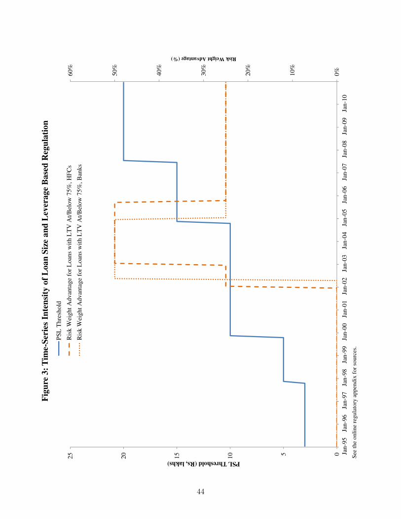
Figure 7 plots the CID measure around 30-day delinquencies, before and after our lender
adopted the reclassification of NPAs. The measure is cross-sectionally demeaned by both
cohort-year and calendar-year, to ensure that we are not picking up cohort or macroeconomic
effects. In both panels of Figure 7, date 0 is the first date that the loan is declared 30-days
delinquent (values below 1 are possible because of the cross-sectional demeaning). The top
panel shows that prior to the change in the regulatory definition of NPAs, loans declared
30-days delinquent on average inflicted a cost on the mortgage provider of roughly 1.1 EMIs
after a year. Post-March 2004, there is a substantial recovery in this number, with such
30-delinquent loans roughly 0.4 EMIs delinquent 12 months later. The bottom panel of the
figure shows that this change in the behavior of the CID after the regulatory redefinition of
NPAs is highly statistically significant.
We undertake this analysis more formally by estimating how changes in the CID vary
following a 30-day delinquency, but prior to hitting the 90-day threshold, both before and
after the regulatory redefinition of the NPA period. To do so, we estimate expected debt
collection rates– changes in the CID– as a polynomial function of the level of the CID prior
to the 90-day delinquency mark (i.e., a CID level of −3), allowing for a jump in the rate at
the 90-day delinquency mark, and modelled as a linear function of the CID beyond the 90-
day delinquency mark. As before, we include time- and cohort-specific fixed effects during
estimation to ensure that we are not merely picking up some of the broader changes detected
earlier in the regulatory and macroeconomic environment.
Figure 8 shows how the estimated debt collection rate varies before and after the 90-day
delinquency threshold, before and after the regulatory reclassification of NPAs was adopted.
The figure reveals that following the adoption of the reclassification, the debt collection
rate prior to hitting the 90-day mark increased substantially relative to the pre-adoption
period, with a significant discontinuity at the 90-day threshold, where the debt collection
rate falls sharply.12 We also consider whether the introduction of SARFAESI had any
12The increase in the debt collection rate prior to the 90-day delinquency mark, and the discontinuity
26
significant impacts on the ability to collect on debts, and find that differences are minimal
and statistically insignificant.
While these changes to debt collection rates are evident in the data, one potential inter-
pretation is that the redefinition of NPAs from 180 to 90 days simply shifted the inevitable
recovery of cash from delinquent borrowers by the 90-day difference between these two dates.
In other words, perhaps the change merely provided a time-value improvement in the net
cash flows of the mortgage provider, but no more substantial impacts.
To address this question, Figure 9 shows the cumulative distribution function (CDF) of
the change in the CID (time- and cohort-demeaned) in the year following the first 30 day
delinquency. This CDF is plotted for three time periods, namely, January 1995 to June
2002, when SARFAESI was first implemented; July 2002 to the date our lender adopted a
reclassification of NPAs; and from this adoption date until the end of the sample period in
2010. We plot the figure on a log scale to focus attention on the very worst cases (i.e., those
loans with the greatest degradation in CID over the year following the date of first 30-day
delinquency), as these loans are the most likely candidates for a complete write-off.
The figure shows that the post-NPA redefinition CDF first-order stochastically dominates
both the pre- and post-SARFAESI CDFs, showing a substantial reduction in the incidence
of high degradation in the CID. While SARFAESI appears to have had some beneficial
impacts for the very worst cases, this is dwarfed by the large impact of the NPA redefinition.
These substantial impacts on eventual bad debts of this regulatory redefinition are striking,
as it appears that there are important benefits to incentivizing mortgage providers to detect
and take early action on delinquencies.
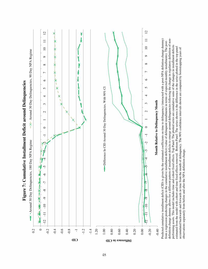
In Figure 10 we document some evidence that the change in the regulatory classification
of NPAs affected screening at mortgage origination as well as mortgage monitoring practices.
This figure reports the same curve as in Figure 9, separately for loans originated in six-month
windows before and after the NPA reclassification was adopted by our lender. The left tail
at that mark are both economically and statistically significant. The online empirical appendix plots thedifference between the pre- and post-adoption debt collection rates with associated bootstrap confidenceintervals.
27
of the distribution is noticeably thicker for loans originated before the reclassification. Since
we are observing delinquency experiences for both cohorts of loans over the same post-
reclassification period (with presumably enhanced monitoring), the reduced probability of
very bad outcomes for loans issued post-adoption is evidence that mortgage screening at
origination was heightened as well.
In summary, a simple change in the regulatory definition of NPAs appears to have signif-
icantly moderated mortgage delinquencies. The impacts are visible in both the probability
of delinquency and the eventual loss given delinquency.
A natural question that arises here is why the lender did not implement such changes
to monitoring voluntarily, earlier than the regulatory imposition of the change, given the
significant impacts on short- and long-term delinquency rates. The issue here is that loan
screening and monitoring are costly, and we do not measure the costs. Given that we do
not (and cannot feasibly) assess these costs, we are unable to assess the net impact on the
lender of implementing quicker action on potentially delinquent loans, despite documenting
that the benefits of such monitoring are large. It is also possible that tougher screening, by
reducing credit extended to lower quality borrowers, conflicts with the lender’s incentives to
lend to the priority sector and may incur political or public relations costs.
5 Conclusion
The Indian regulatory and macroeconomic environment has changed dramatically during
the last two decades. A fast-developing housing finance system has coped with significant
variation in default rates and interest rates, and regulatory changes in the incentives to
originate mortgages in general, and small loans in particular. In this paper we have explored
the effects of such regulatory changes on mortgage risk using an empirical strategy that
links time variation in regulation with expected cross-sectional impacts on different types of
mortgages.
We have presented evidence that regulatory subsidies for low-cost housing and less lever-
aged loans are associated with higher delinquencies, controlling for interest rates at loan
28
issuance, and that changes to the definition of non-performing assets impacted behavior in
response to early evidence of payment delinquencies. While it is diffi cult to generalize find-
ings from one country, or to make welfare statements in the absence of a full estimation of
both costs and benefits, our findings on the infrequent adjustment of PSL-thresholds suggest
that paying attention to the design of policies may yield rewards, and the estimated effect of
the regulatory redefinition of NPAs suggests that even seemingly minor regulatory changes
can have important impacts on mortgage monitoring and origination practices, and hence
on mortgage risk.
29
References
Acharya, Viral V., Matthew Richardson, Stijn van Nieuwerburgh, and Lawrence J. White,
2011, Guaranteed to Fail: Fannie Mae, Freddie Mac, and the Debacle of Mortgage
Finance, Princeton University Press, Princeton, NJ.
Adelino, Manuel, Kristopher Gerardi, and Paul S. Willen, 2013, “Why Don’t Lenders Rene-
gotiate More Home Mortgages? Redefaults, Self-Cures, and Securitization”, Journal
of Monetary Economics 60, 835—853.
Adelino, Manuel, Antoinette Schoar, and Felipe Severino, 2014, “Credit Supply and House
Prices: Evidence from Mortgage Market Segmentation”, unpublished paper, Duke
University and MIT.
Agarwal, Sumit, Gene Amromin, Itzhak Ben-David, Souphala Chomsisengphet, and Dou-
glas D. Evanoff, 2011, “The Role of Securitization in Mortgage Renegotiation”, Journal
of Financial Economics 102, 559—578.
Agarwal, Sumit, Efraim Benmelech, Nittai Bergman, and Amit Seru, 2012, “Did the Com-
munity Reinvestment Act (CRA) Lead to Risky Lending?”, NBERWorking Paper No.
18609.
Aghion, Philippe, Robin Burgess, Stephen J. Redding, and Fabrizio Zilibotti, 2008, “The
Unequal Effects of Liberalization: Evidence from Dismantling the License Raj in In-
dia”, American Economic Review, 98(4), 1397—1412.
Amromin, Gene, Jennifer Huang, Clemens Sialm, and Edward Zhong, 2011, “Complex
Mortgages,”NBER Working Paper No. 17315.
Anagol, Santosh, and Hugh Kim, 2012, “The Impact of Shrouded Fees: Evidence from a
Natural Experiment in the Indian Mutual Funds Market”, American Economic Review,
102(1), 576-593.
30
Avery, Robert, and Ken Brevoort, 2011, “The Subprime Crisis: Is Government Housing
Policy to Blame?,”FEDS Working Paper 2011-36, Federal Reserve Board.
Baily, Martin N., 2011, ed., The Future of Housing Finance: Restructuring the U.S. Resi-
Table 3: Summary Statistics on Loan Characteristics by Disbursal Year
Loan Term (Years)Initial Interest Rate Loan-Cost Ratio Loan-Income Ratio
Loan Term (Years)Initial Interest Rate Loan-Cost Ratio Loan-Income Ratio Cohort 90-Day Delinquency Rate
This table provides equal-weighted yearly means (Panel A) and standard deviations (Panel B) of important characteristics for the more than 1.2
million mortgage loans disbursed by the lender. Cohort delinquency rates are computed as the annual probability that an outstanding and not-yet-90-
day-delinquent loan experiences a 90 day delinquency. This probability is computed separately for each disbursal-year cohort and calendar year. The
delinquency rate below represents the time-series average across calendar year estimates for each disbursal-year cohort. Statistics for fixed rate
disbursals are removed for the years 2008 through 2010, as fixed rate disbursals account for well under one percent of disbursals (by count or value) in
each of these years. Similarly, cohort 90-day delinquency rate is omitted for loans disbursed after 2007 as these loans have not been around long
Using a Three-month Time Window Around Risk Weight Changes
Table 6: Impact of Risk Weight Regulation on Abnormal Delinquency Rate
This table provides parameters of interest from the combination of Equations 1 (in section A) and Equation
8 (in section B) in the paper estimated as Cox hazard models on the population of loans disbursed around a
75% loan-cost ratio around the time of risk weight changes for loans below 75% loan-to-value. In section
A, the reported values are differences in abnormal delinquency rates on loans disbursed below and above a
75% loan-cost ratio under regimes where risk weights on loans disbursed around that threshold are [i]
relatively far and [ii] relatively close. In section B, the coefficient η represents the impact of the risk weight
advantage carried on less leveraged loans (100% minus the risk weight on these loans) on abnormal
delinquency rates. Coefficients and standard errors are scaled to reflect the impact relative to the average
delinquency rate in the full loan sample. Standard errors (reported in parentheses) are computed by
bootstrapping years of the panel data, with bold and italicized type representing statistical significance at
the five and ten percent level respectively.
Using a Six-month Time Window Around Risk Weight Changes
B. Abnormal Delinquencies as a Function of Risk Weight Advantage (Equation 8)
Using a Three-month Time Window Around Risk Weight Changes
A. Difference-in-Difference Specification (Equation 1)
Using a Six-month Time Window Around Risk Weight Changes
Using a Three-month Time Window Around Risk Weight Changes
Using a Six-month Time Window Around Risk Weight Changes
[i]: τ���,��� − τ���,����
[ii]: τ ���,��� − τ ���,����
[i]: τ���,��� − τ���,����
[ii]: τ ���,��� − τ ���,����
40
Month Relative
Probability of 30 day
Delinquency Transitioning to
90 day Delinquency
Probability of 90 day
Delinquency Transitioning to
180 day Delinquency
For Initial Delinquencies Occurring:
All Months (Jan 1996-Dec 2010) 22.7% 22.8%
(0.3%) (0.4%)
Lender Under 180day NPA Regime 29.2% 23.5%
(0.5%) (0.6%)
Lender Under 90day NPA Regime 16.0% 22.2%
(0.5%) (0.6%)
Difference -13.3% -1.3%
(0.7%) (0.9%)
Table 7: Probability of Transition to Later Stage of DelinquencyThis table presents the probability that initial 30 and 90 day mortgage delinquencies become 90 and 180
day mortgage delinquencies respectively within six months following the initial delinquency. This
transition probability is first computed for all loans with initial delinquencies in a given month, and the
probabilities shown below are the time-series average of these monthly cross-sectional estimates, where
the average is taken over the indicated time periods. Standard errors are reported in parentheses below
estimates and are constructed by bootstrapping from the population of monthly cross-sectional estimates
from each time period indicated. All coefficients except the differences in 90 to 180 day default transition
probabilities are highly statistically significant.