Remote Sens. 2014, 6, 12866-12884; doi:10.3390/rs61212866

remote sensing ISSN 2072-4292

www.mdpi.com/journal/remotesensing

Article

The Impact of Time Difference between Satellite Overpass and Ground Observation on Cloud Cover Performance Statistics

Jędrzej S. Bojanowski *, Reto Stöckli, Anke Tetzlaff and Heike Kunz

Federal Office of Meteorology and Climatology MeteoSwiss, Climate Services, Operation Center 1,

P.O. Box 257, CH-8058 Zürich-Flughafen, Switzerland; E-Mails: reto.stoeckli@meteoswiss.ch (R.S.);

anke.tetzlaff@meteoswiss.ch (A.T.); heike.kunz@meteoswiss.ch (H.K.)

* Author to whom correspondence should be addressed; E-Mail: jedrzej.bojanowski@meteoswiss.ch;

Tel.: +41-58-460-93-56.

External Editors: Alexander Kokhanovsky and Prasad S. Thenkabail

Received: 20 October 2014; in revised form: 8 December 2014 / Accepted: 15 December 2014 /

Published: 22 December 2014

Abstract: Cloud property data sets derived from passive sensors onboard the polar orbiting

satellites (such as the NOAA’s Advanced Very High Resolution Radiometer) have global

coverage and now span a climatological time period. Synoptic surface observations

(SYNOP) are often used to characterize the accuracy of satellite-based cloud cover.

Infrequent overpasses of polar orbiting satellites combined with the 3- or 6-h SYNOP

frequency lead to collocation time differences of up to 3 h. The associated collocation error

degrades the cloud cover performance statistics such as the Hanssen-Kuiper’s discriminant

(HK) by up to 45%. Limiting the time difference to 10 min, on the other hand, introduces

a sampling error due to a lower number of corresponding satellite and SYNOP observations.

This error depends on both the length of the validated time series and the SYNOP frequency.

The trade-off between collocation and sampling error call for an optimum collocation time

difference. It however depends on cloud cover characteristics and SYNOP frequency, and

cannot be generalized. Instead, a method is presented to reconstruct the unbiased (true) HK

from HK affected by the collocation differences, which significantly (t-test p < 0.01)

improves the validation results.

Keywords: validation; collocation; SYNOP; AVHRR; sampling error; cloud retrieval;

ESA-Cloud-CCI; APCADA; skill score; Hanssen-Kuiper’s discriminant

OPEN ACCESS

Remote Sens. 2014, 6 12867

1. Introduction

Clouds have a major impact on the Earth’s radiation budget, and, thus, play a crucial role in the

terrestrial climate system [1]. They cool the atmosphere by reflecting the incoming solar radiation.

Concurrently, they warm the atmosphere by intercepting and radiating back the radiation emitted by the

Earth’s surface. The net radiative effect of a cloud depends on its physical properties [2], and cloud

feedbacks are among the most uncertain components of the climate models. Consistent and continuous

cloud observations are required to better understand the cloud-climate interactions. Therefore, as part of

the United Nations Framework Convention on Climate Change (UNFCCC), the Global Climate Observing

System (GCOS) has included cloud properties in the set of essential climate variables (ECVs) [3] with a

special emphasis on satellite-based retrievals [4].

Polar-orbiting satellites provide a global coverage of cloud information at sub-daily time resolution.

This feature has been exploited for deriving cloud climatologies by, for example, the International Satellite

Cloud Climatology Project (ISCCP) [5], Pathfinder Atmospheres Extended (PATMOS-x) [6,7], and the

EUMETSAT Satellite Application Facility on Climate Monitoring (CM SAF) [8] to produce the CLoud,

Albedo and RAdiation dataset (CLARA-A1) [9]. Recently, the European Space Agency (ESA) has

initiated the ESA-Cloud-CCI project focused on cloud studies in the frame of its Climate Change

Initiative (CCI) running over the time period of 2010 to 2016 [10]. The ESA-Cloud-CCI aims at adapting

and developing the state-of-the-art cloud retrieval schemes [11] to be applied to the longest existing time

series of the cloud observations available from polar orbiting satellites with AVHRR and AVHRR-like

sensors [12]. The cloud properties (i.e., cloud cover, cloud top height and temperature, cloud optical

thickness, cloud effective radius, and liquid and ice water paths) are derived by means of an

optimal-estimation-based retrieval framework [13] for: (1) the Advanced Very High Resolution

Radiometer (AVHRR) heritage product (1982–2014) comprising (Advanced) Along Track Scanning

Radiometer (A)ATSR, AVHRR and Moderate-Resolution Imaging Spectroradiometer (MODIS), and

(2) the (A)ATSR-Medium Resolution Imaging Spectrometer (MERIS) product (2002–2012) [14].

In order to be useful for the climate studies, the satellite-based cloud datasets must fulfil quality

requirements defined by GCOS [4]. The quality assessment is based on a comparison with the

ground-based observations or other satellite-based datasets. The active sensors onboard CloudSat [15]

and CALIPSO [16] have proved beneficial for the validation of passive radiometers with their ability to

reveal the vertical cloud structure [17]. However, their scarce spatio-temporal coverage limits the number of

possible collocations, thus, the active sensor data is more useful for cloud retrieval algorithm development

than as a reference for cloud climatology datasets. The conventional surface observations (SYNOP) still

remain a common reference for the validation of cloud cover from passive sensors [18–24].

There are several sources of uncertainty when validating satellite-derived cloud cover with

ground-based synoptic observations [25]. A different viewing perspective (the uppermost cloud layer

seen by the satellite versus the lowest layer observed from the ground) can cause significant discrepancy

in case of multi-layer clouds [26–28]. Further uncertainty can be caused by a different spatial footprint

(the passive sensor’s spatial resolution of 1–5 km versus synoptic observations limited by the typical

range of vision of 30–50 km [29]), as well as by a different sensitivity of a satellite sensor and the human

eye (a cloud of certain optical thickness may be visible for the observer but remain transparent for the

sensor, and vice versa). Moreover, the uncertainty increases towards the edges of the field of view for

Remote Sens. 2014, 6 12868

satellite observation, and towards the horizon for visual observation. Further, satellite-based cloud

retrieval algorithms usually provide binary information (cloudy or cloudless), while ground observations

report the part of the visible sky covered by clouds with an accuracy of 1/8 (okta). In addition, the okta

scale is not linearly related to cloud cover. As soon as a cloud is visible, even covering less than 1/8 of

the sky, at least 1 okta is reported. Similarly, a small discontinuity in the cloud cover (clear sky of less

than 1/8 of the sky) is reported as 7 okta [30–32]. Between 2 and 6 okta, the synoptic observations should

reflect the part of the sky covered by clouds. All the mentioned different features of the spaceborne and

ground cloud cover observations can affect the validation results, even if both observations match

perfectly in time.

However, satellite-based measurements and reference ground-based cloud cover observations are discrete

and usually not performed at the same time. Particularly, the observation time difference occurs when

comparing cloud retrievals from polar orbiting satellite data with irregular overpass times to 3- or 6-h

SYNOP observations. A maximum collocation time difference between these two types of observations

has to be chosen. It strongly varies among the validation activities: e.g., 15 min [33], 1 h [18], or 4 h [24].

Fontana et al. [20] used an average of the synoptic observations at 9UTC and 12UTC, and of 12UTC

and 15UTC to validate cloud cover from the Terra-MODIS morning acquisition and the Aqua-MODIS

afternoon acquisition, respectively. Kotarba [22] set the maximum time difference between the MODIS

cloud mask and SYNOP to 30 min, but, in addition, normalized the SYNOP observations to MODIS

overpass times using a linear interpolation. To avoid this discrepancy some authors perform the

validation only based on the daily or monthly averages [19].

The choice of a small time difference (e.g., 10 min) ensures that both observations (satellite and

SYNOP) reflect the same cloud state. However, such a choice strongly limits the number of satellite

overpasses, which have a corresponding SYNOP observation. As a consequence only a subsample of all

satellite observations can be used for the validation, which introduces a sampling error. On the other

hand, the maximum time shift of 90 min for 3-h SYNOP (180 min for 6-h SYNOP) allows the use of all

satellite overpasses and minimizes the sampling error, but at the expense of introducing an error due to

the incomparability of the cloud states separated by up to 90 (or 180) min. In this context, defining the

optimal maximum time difference between satellite and ground observations requires the compromise

between sampling and incomparability errors.

The main objective of this paper is to quantify and demonstrate the impact of this time difference on

validation results of satellite-derived cloud cover. This could be studied on the actual satellite-derived

cloud cover data (such as the ESA-Cloud-CCI). Then, however, the assessment would be limited to the

accuracy of the chosen satellite-based cloud cover; the validation of the ESA-Cloud-CCI is not the scope

of this paper. In order to assess the impact for the range of possible accuracies (from perfect to low skill)

an idealized study is performed. The validation dataset is composed of 10-min cloud amount estimates,

time of ground observations (SYNOP), and real NOAA/AVHRR overpass times. It allows to analyze

the impact of the time difference with a 10-min step, which would not be possible using 3-h SYNOP

instead. After quantifying the sampling and incomparability errors on validation results, we introduce

and evaluate a method for modeling the unbiased (true) validation results, as they would be derived

without any time shift between satellite overpass and reference ground observation.

Remote Sens. 2014, 6 12869

2. Data

2.1. Ground-Based Cloud Cover Observations

The ground-based data were obtained from the Baseline Surface Radiation Network (BSRN) [34]. BSRN

is a project of the World Climate Research Programme (WCRP) and the Global Energy and Water

Experiment (GEWEX). The project objective is to provide high-quality measurements of short-wave and

long-wave surface radiation fluxes with a 10-min interval at stations located in the various climatic

zones. These measurements are accompanied by measurements of air temperature, relative humidity and

air pressure.

Long-wave downward radiation, air temperature and humidity measurements allow to determine the

so-called partial cloud amount based on the Automatic Partial Cloud Amount Detection Algorithm

(APCADA). APCADA was developed by Marty and Philipona [35] and further enhanced by Dürr and

Philipona [36]. It derives cloud amount from the ratio of the all- and clear-sky long-wave emittance.

Since most of the long-wave emittance measured at the surface originates from the first kilometer of the

atmosphere [37,38], high clouds have a limited effect on the down-welling long-wave radiation.

Therefore, APCADA cloud amount, similar to most passive satellite datasets, may underestimate the

amount of thin high clouds. Dürr and Philipona [36] estimated that in 82%–87% (for six high-latitude

and mid-latitude sites) and 77% (for one tropical site) of the observations the maximum difference

between the APCADA and SYNOP observations was smaller or equal to 1 okta.

APCADA was employed in this study to estimate cloud amount at 10 BSRN sites at a 10-min

resolution (Table 1). The sites covered the range of different climatic zones (Figure 1). The cloud regime

at each site was characterized by the annual average and temporal variability of cloudiness. The latter

was calculated as the percent of changes in cloudiness (cloudy-cloudless) in the total number of

observations. The mean cloudiness and cloudiness variability depend on the APCADA accuracy and

cloud cover classification. Therefore, they are provided herein to assist the interpretation of the results,

but they should not be treated as climate indices.

Table 1. The Baseline Surface radiation Network (BSRN) sites used in the study. The

cloudiness temporal variability indicates the percent of changes in cloudiness (from cloudy

to cloudless and vice versa) in the total number of observations.

Site Name Country Lat (Deg) Lon (Deg)Elevation

(m a.s.l.)

Mean

Cloudiness (%)

Cloudiness Temporal

Variability (%)

Bermuda Bermuda 32.27 N 64.68 W 8 67 24

Cabauw Netherlands 51.97 N 4.93 E 0 68 20

De-Aar South-Africa 30.66 S 23.99 E 1287 29 16

Lindenberg Germany 52.21 N 14.12 E 125 70 17

Ny-Ålesund Norway 78.93 N 11.93 E 11 74 13

Palaiseau France 48.71 N 2.20 E 156 63 18

Payerne Switzerland 46.81 N 6.94 E 491 66 17

Sede-Boqer Israel 30.90 N 34.78 E 500 40 28

Solar Village Saudi Arabia 24.91 N 46.41 E 650 23 14

South-Pole Antarctica 89.98 S 24.79 W 2800 73 10

Remote Sens. 2014, 6 12870

Figure 1. The Baseline Surface Radiation Network (BSRN) sites overlaid on the

Köppen-Geiger map of climate zones [36]: 1-Bermuda, 2-Cabauw, 3-De-Aar, 4-Lindenberg,

5-Ny-Ålesund, 6-Palaiseau, 7-Payerne, 8-Sede-Boqer, 9-Solar-Village, and 10-South-Pole.

2.2. Satellite Overpass Times

The satellite data were obtained from the ESA-Cloud-CCI 3-year (2007–2009) [39,40] prototype

cloud properties dataset derived from the AVHRR global area coverage (GAC) [41] in the first project

phase. The Level 2G AVHRR GAC data is gridded from the Level 2 swath data by taking only the

most-nadir observation in polar regions, where Level 2 swaths overlap. Using separate day- and

night-time Level 2G grids for four NOAA polar satellite platforms (NOAA 15–18) result in eight

observations per day and per grid point. Thus, the time series for every site contained 8768 image

acquisition times (three years × eight overpasses). The cloud cover and properties were not extracted,

but only the exact overpass times (in seconds) at each BSRN site.

3. Methods

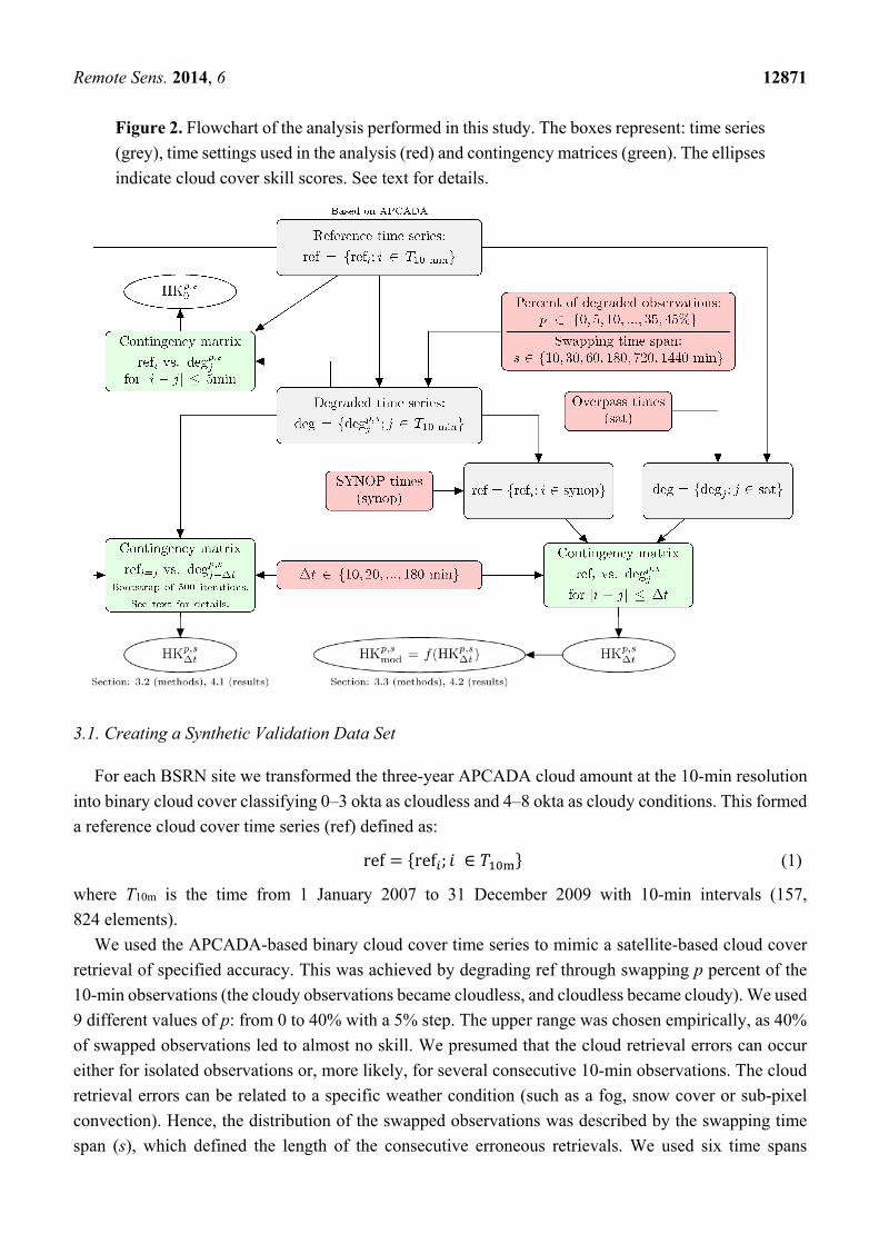
In this section we describe the main steps of the analysis following the flowchart shown in Figure 2.

Remote Sens. 2014, 6 12871

Figure 2. Flowchart of the analysis performed in this study. The boxes represent: time series

(grey), time settings used in the analysis (red) and contingency matrices (green). The ellipses

indicate cloud cover skill scores. See text for details.

3.1. Creating a Synthetic Validation Data Set

For each BSRN site we transformed the three-year APCADA cloud amount at the 10-min resolution

into binary cloud cover classifying 0–3 okta as cloudless and 4–8 okta as cloudy conditions. This formed

a reference cloud cover time series (ref) defined as: ref = ref ; ∈ (1)

where T10m is the time from 1 January 2007 to 31 December 2009 with 10-min intervals (157,

824 elements).

We used the APCADA-based binary cloud cover time series to mimic a satellite-based cloud cover

retrieval of specified accuracy. This was achieved by degrading ref through swapping p percent of the

10-min observations (the cloudy observations became cloudless, and cloudless became cloudy). We used

9 different values of p: from 0 to 40% with a 5% step. The upper range was chosen empirically, as 40%

of swapped observations led to almost no skill. We presumed that the cloud retrieval errors can occur

either for isolated observations or, more likely, for several consecutive 10-min observations. The cloud

retrieval errors can be related to a specific weather condition (such as a fog, snow cover or sub-pixel

convection). Hence, the distribution of the swapped observations was described by the swapping time

span (s), which defined the length of the consecutive erroneous retrievals. We used six time spans

Remote Sens. 2014, 6 12872

(for p > 0%): 10, 30, and 60 min, and 3, 12 and 24 h. The swapping blocks were then randomly distributed

along the ref time series. We defined the degraded time series as: deg , = deg , ; ∈ (2)

Thus, for instance, deg %, indicates a degraded reference time series where 5% of the

observations in 3-h blocks were swapped.

For each of the 10 sites one reference time series (ref) and 49 degraded time series (deg) were generated: they combined 8 p’s greater than 0% with 6 s’s and were extended by deg % (equal to ref),

which was the artificial cloud retrieval of a perfect skill. The lowest skill was represented by deg %.

3.2. Validation Procedure

The reference (ref) and degraded (deg) time series were used to analyze the theoretical impact of time

difference between satellite overpass and ground observation on the satellite-derived cloud cover

performance. The exact times of the NOAA 15–18 overpasses were used, and the SYNOP observations

were assumed to be carried out routinely every 3 or 6 h.

The performance of each deg was measured by a skill score commonly referred to as the

Hanssen-Kuiper’s Discriminant formulated as [42]: HK = −( + )( + ) = − (3)

where a (correct detections), b (false alarms), c (misses) and d (correct no-detection) build a contingency

matrix (Table 2). HK can be also formulated as a difference between the hit rate: H = a/(a + c), and the

false alarm rate: F = b/(b + d). We derived HK only for a contingency matrix of the number of samples

(a + b + c + d) equal or greater than 10. A perfect cloud detection receives the score of one, random

retrieval the score of zero, and inferior to random a negative score. HK equals zero for the constant

detection of the cloudy or cloudless conditions. Furthermore the contribution made by a correct miss or

a correct detection increases as the event is more or less likely, respectively [42]. Thus, HK also reflects

the skill of detecting rare events, which makes it more robust than, e.g., the H and F alone.

Table 2. A contingency matrix for the evaluation of the satellite-based cloud cover against

reference observations.

Ground Observation

Cloudy Cloud-Free

Satellite Cloudy a b

Cloud-free c d

The validation procedure was performed for each station and degraded time series (deg). First the

unbiased (true) skill score (HK0) was calculated assuming no time difference between deg (simulating

the satellite image acquisition) and ref (simulating the reference SYNOP observation). Only a subset of

the 10-min time steps, closest to the actual satellite overpass times during three years, were used to derive

HK0. We notate “HK0” for simplicity, however the time difference for HK0 was not exactly equal zero,

but did not exceed 5 min.

Remote Sens. 2014, 6 12873

Next we performed the validation of each deg assuming a time difference (Δt) between satellite

overpass and SYNOP from 10 to 90 min (for 3-h SYNOP) or 10 to 180 min (for 6-h SYNOP) with a 10-min

step. To assess the impact of Δt on HK we validated degj=i against refi+Δt: both the satellite-derived and

reference observations were shifted by Δt. For each Δt the number of satellite overpasses (n) corresponding

to the SYNOP observations with a time difference below or equal Δt were determined. The sampling

error for n being lower than the total number of overpasses (N) was estimated with the bootstrap

technique [43]: HKΔt was derived 500 times from n observations randomly chosen from all satellite

overpasses. As a result for each site: SYNOP frequency, percent of swapped observations (p), swapping

time span (s), and time difference (Δt) 500 HK’s were derived. They were compared with HK0 to assess

the impact of the time difference, sampling size and cloud regime of the site on the validated HK.

3.3. Modeling the Unbiased Skill Score

To examine how accurately the unbiased HK0 can be reconstructed from the HK’s affected by Δt, the

validation procedure was modified and performed based on the actual collocations between the satellite

overpasses and ground observations for certain Δt’s (while previously only the number of collocations n

was used, and ref and deg where shifted by Δt). APCADA-based cloud cover was extracted for each

degp,s only at the satellite overpass times, and for each ref only at the SYNOP observation times. Then,

HKΔt was calculated for the range of different maximum Δt. This way the sampling error was not assessed

(unlike before by the bootstrap), but it impacted each HK derived with a given Δt. HK0 was derived with

the method described in the previous section.

Next, we modeled the unbiased skill score (HKmod) from the 9 (for 3-h SYNOP) or 18 (for 6-h

SYNOP) HKΔt’s. First, using a least square regression we fitted a linear function f to the HKΔt’s: HK∆ = (∆ ), ∆ ∈ 10,20,… ,90/180 min (4)

Then HKmod was calculated as: HKmod = (∆ = 0) (5)

To evaluate HKmod the commonly used performance statistics such as the mean bias error, mean

absolute error, and root mean square error were calculated against the unbiased skill score HK0.

The significance of the differences between performances of the validation methods was tested with

a two-sided t-test for unpaired samples.

4. Results

4.1. Characterizing the Skill Score Uncertainty

The maximum time difference (Δt) between satellite overpass and SYNOP observation has a twofold

effect on the obtained skill score. An increase of Δt causes: (1) an increase in the absolute bias of HKΔt

as compared to HK0, and (2) a decrease in spread of the retrieved HKΔt. An example for Payerne shown

in Figure 3 illustrates these two effects. The bias increasing with Δt is represented by the difference

between the median HKΔt (i.e., the horizontal line within each box) and HK0 marked as ×. The spread in

HKΔt is represented by the box height and its whiskers range. The upper axis gives the number of samples

(n) used for calculating HKΔt selected from all overpasses (N).

Remote Sens. 2014, 6 12874

Figure 3. An example of the validation results at Payerne for the degraded time series

(degp = 1°%,s = 3h) for a different maximum time difference between the NOAA/AVHRR

overpass and reference SYNOP observation (Δt). Each boxplot contains 500 values derived

from the random selection of n samples from the total number of overpasses (N = 7589). The

unbiased skill score (HK0) is marked with ×. The boxes contain the median (thick line), their

bottom and top identify the 1st and 3rd quartiles, and the whiskers extend to the data extremes.

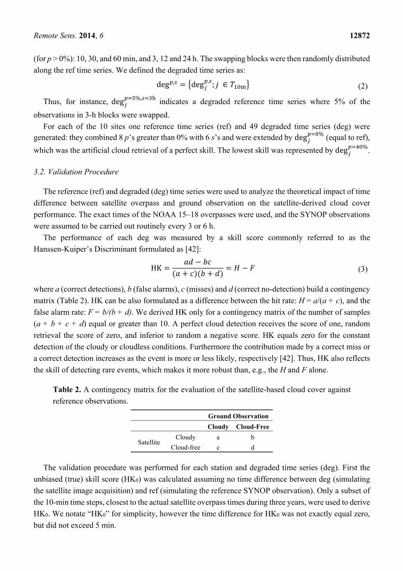
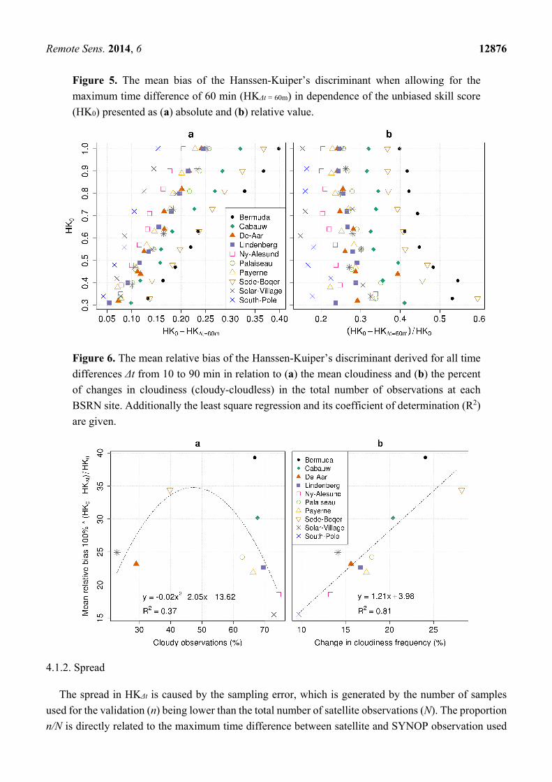
4.1.1. Bias

Figure 4 illustrates how the bias of HK (HK0 − HKΔt) increases with an increase of Δt, and more

rapidly for high skill scores (e.g., the red boxes representing the time series of a perfect skill) than for

low skill scores (e.g., the magenta boxes representing the time series of HK0 of around 0.35). For instance

(Figure 5a), at Bermuda the mean bias at the 60-min time difference is 0.39 for the perfect skill

(HK0 = 1) and only 0.13 for the lowest skill analysed (HK0 ≈ 0.3). Yet, this range in the bias of HK

differs among the sites. Bermuda reveals the biggest difference of 0.26 (0.39 − 0.13) and the South Pole

has the lowest one of 0.11 (from 0.15 for HK0 = 1 to 0.04 for HK0 ≈ 0.35). However, the bias calculated

in relation to the unbiased skill score (relative bias) is nearly constant for HK0 greater than 0.5 at each

site and for a given time difference (i.e., 60 min in Figure 5): it ranges from around 0.1 for the South

Pole to around 0.42 for Bermuda (Figure 5b).

The sites with medium cloudiness are more sensitive to the time difference (Δt) than sites of high and

low cloudiness. Figure 6 shows the mean relative bias calculated for all analyzed time differences Δt at

each site. Again, the extreme cases are: Bermuda of 67% of cloudiness, where the time difference causes

the underestimation of the unbiased skill score by nearly 40%, and the South Pole, of 73% of cloudy

observations, where the underestimation is only 15%. Among the analyzed sites the South Pole has the

highest persistence of cloudiness with only 10% change in the cloudiness frequency, while Bermuda

reveals a high change of cloudiness frequency of 24%. The relation of mean cloudiness and cloud

variability with the relative bias in HK can be explained by the fact that, for sites with constant cloudy

or clear-sky conditions, it is unlikely that time difference introduces a bias in the skill score. However the

correlation between the cloudiness (and the frequency of change in cloudiness) and the relative bias is too

low (Figure 6) for allowing the cloudiness characteristics to be a generalized predictor of the HK bias.

Remote Sens. 2014, 6 12875

Figure 4. The validation results for the degraded time series with a varying maximum time

difference between NOAA/AVHRR overpass and reference SYNOP observation (Δt). The

degraded time series (degp,s) are of the swapped time span (s) equal 12 h, and the percent of

swapped observations (p) of: 0% (red), 10% (green), 20% (blue), 30% (cyan), and 40%

(magenta). Each boxplot contains 500 values derived from the random selection of n samples

from the total number of overpasses (N = 7589). The unbiased skill score (HK0) is marked

with ×. The boxes identify the first and third quartiles, and the whiskers extend to the

data extremes.

Remote Sens. 2014, 6 12876

Figure 5. The mean bias of the Hanssen-Kuiper’s discriminant when allowing for the

maximum time difference of 60 min (HKΔt = 60m) in dependence of the unbiased skill score

(HK0) presented as (a) absolute and (b) relative value.

Figure 6. The mean relative bias of the Hanssen-Kuiper’s discriminant derived for all time

differences Δt from 10 to 90 min in relation to (a) the mean cloudiness and (b) the percent

of changes in cloudiness (cloudy-cloudless) in the total number of observations at each

BSRN site. Additionally the least square regression and its coefficient of determination (R2)

are given.

4.1.2. Spread

The spread in HKΔt is caused by the sampling error, which is generated by the number of samples

used for the validation (n) being lower than the total number of satellite observations (N). The proportion

n/N is directly related to the maximum time difference between satellite and SYNOP observation used

Remote Sens. 2014, 6 12877

for validation. Therefore, a higher Δt increases n and consequently lowers the spread in HKΔt (Figure 4).

Figure 4 reveals that the spread in HKΔt also depends on its own mean: the greater the mean HK, the

lower the spread. Moreover, sites of low cloudiness variability such as, e.g., the South Pole, are

characterized by the overall lower spread of HK than sites of high cloudiness variability, such as

Sede-Boqer or Bermuda (Figure 4).

Figure 7. Validation results for artificial 3-year time series degp,s of NOAA/AVHRR with

eight overpasses per day against 3-h SYNOP at 10 BSRN sites. HK0 stands for the unbiased

skill score. The blue crosses represent the modeled skill score (HKmod). The red circles

represent the skill score derived by a standard validation, for which the closest SYNOP

observation is used to validate the satellite-derived data (equal HKΔt=90m as for 3-h SYNOP).

4.2. Retrieving the Unbiased Skill Score

The modeled Hanssen-Kuiper’s discriminant (HKmod) was linearly extrapolated from HKΔt’s derived

for Δt from 10 min to 90 or 180 min for 3-h and 6-h SYNOP respectively. When 3 years of NOAA/AVHRR

data with eight overpasses a day are validated against 3-h SYNOP (Figure 7), HKmod is significantly (t-test

p < 0.01) more accurate than the one derived by the standard validation (HKΔt = 90 m). The mean bias error

Remote Sens. 2014, 6 12878

and root mean square error are both improved for all the stations. The underestimation of HKΔt = 90m is

stronger for the time series of higher accuracy (higher HK0), while HKmod remains unbiased over the full

accuracy range. HKmod has the average mean absolute error of 0.03, which is significantly

(t-test p < 0.01) lower than 0.12 for HKΔt = 90 m (Table 3, first row). However, the validation performed

with the maximum time difference of 10 min (HKΔt = 10m) is equally accurate to HKmod (0.01 difference

between the two methods is not significant).

Table 3. The mean absolute bias (MAE) in the Hanssen-Kuiper’s discriminant measured

against the unbiased skill score (HK0) at 10 BSRN sites depending on SYNOP observations

frequency, time series length, and number of satellite overpasses per day. The validation

methods are: four using different maximum time differences between the satellite observation

and SYNOP (HKΔt = 10m, HKΔt = 30m, HKΔt = 60m, and HKΔt = 90m), and the modeled skill score

(HKmod). The values highlighted in bold font indicate the best performance. N gives the

number of satellite observations per station, and n gives the number used for the validation

depending on the validation method.

Time Series

Length

Overpasses

Per Day

SYNOP

Frequency N HKΔt=10m HKΔt=30m HKΔt=60m HKΔt=90m HKmod

n MAE n MAE n MAE n MAE n MAE

3 years 8 3-h 7589 815 0.04 2433 0.07 4962 0.10 7589 0.12 7589 0.03

3 years 8 6-h 7589 399 0.05 1076 0.07 2050 0.10 3302 0.13 3302 0.04

1 year 2 3-h 646 69 0.09 191 0.08 410 0.10 646 0.12 646 0.07

1 month 2 3-h 53 6 - * 15 0.24 34 0.19 53 0.19 53 0.34

* not available because HK is calculated only for n ≥ 10.

The above results were based on the validation of three-year time series with eight overpasses a day

against 3-h SYNOP. The size of both the validated and reference data sets can vary with, e.g., the period

covered, number of satellite overpasses per day and SYNOP observation frequency. The length of the

satellite-based time series (days covered × number of overpasses) defines the number of satellite

observations to be validated (N). The frequency of satellite and SYNOP observations and their

co-distribution in time determine the number of observations used for the validation (n) in dependence

of the maximum time difference between the observations of satellite and SYNOP (Δt).

The performance of both HKmod and HKΔt depends on the temporal coverage and frequency

characteristics of the employed satellite and ground data set (Table 3). HKmod outperforms HKΔt

(according to the MAE) for three out of four analyzed settings. Only for the shortest time series covering

one month the standard validation using a 30-min maximum time difference between the satellite and

SYNOP observations (HKΔt=30m) provides the most accurate HK. For such short validation time series

HKmod cannot be reconstructed from HKΔt. Also, the example for Payerne (Figure 8) shows the

concurrent high uncertainty of HK. It is caused by the greater sampling error for few collocations

(as explained in Section 4.1.2). This example suggests that the validation of cloud cover data from a

single polar orbiter and using SYNOP as a reference should encompass at least one year.

Remote Sens. 2014, 6 12879

Figure 8. The bias in Hanssen-Kuiper’s discriminant measured against the unbiased skill

score (HK0) at Payerne depending on the SYNOP observation frequency, time series length,

and number of satellite overpasses per day. The bias is reported for four different maximum

time differences between the satellite observation and SYNOP (HKΔt=10m, HKΔt=30m, HKΔt=60m,

and HKΔt=90m), and for the modeled skill score (HKmod, orange). The missing box is due to

n < 10 for which HK is not calculated. The boxes contain a median (thick line), their bottom

and top identify the 1st and 3rd quartiles, and the whiskers extend to the data extremes.

5. Discussion

5.1. Validation Inaccuracy

The choice of a maximum time difference between the satellite observation and reference SYNOP

used for the validation has a significant impact on the validation accuracy. Limiting the time difference

to, e.g., 10 min increases the comparability of both datasets and has a positive impact on the validation

accuracy. On the other hand, a low maximum time difference significantly lowers the number of possible

collocations. For a maximum time difference of 10 min, only 10% of satellite observations can be used

for validation. The resulting increase of the sampling error has a negative impact on the validation accuracy.

The decrease of comparability between the validated and reference data with an increasing time

difference introduces a negative bias, as the derived skill score is underestimated. This bias is stronger

for the time series of higher accuracy, and becomes less important for the time series of low skill.

Remote Sens. 2014, 6 12880

Our findings demonstrate that the very high skill scores (with a HK close to 1.0) cannot be reported with

the traditional validation employing a single fixed maximum time shift.

Since the maximum time difference has two opposing (positive and negative) effects, a compromise

has to be found. However, our analysis reveals the complexity of this impact on the validation accuracy:

it depends on the accuracy, temporal characteristics and extent of the satellite data set, on the cloudiness

and its variability, as well as on the frequency of the reference SYNOP observations. We were not able

to find a generalized function to define the optimal time difference for the standard validation. Instead

we propose a method to reconstruct the unbiased skill score.

5.2. Modeling Unbiased Skill Score

The parametric model for the unbiased skill score (calculated without time difference between the

satellite and SYNOP observations) is based on the extrapolation of a linear curve fitted to the HK’s

derived with several time differences. This method does not require any auxiliary data. It only employs

the satellite observations and SYNOP. We demonstrate that the modeled skill score is more accurate

than the one derived by the standard validation procedures unless the sampling error becomes very large

at small sample sizes. In this particular case, however, none of the validation methods yields satisfactory

results. The method presented here can reduce the validation error caused only by the incomparability

of the observations due to the shift in time.

6. Conclusions

This study reveals the often-disregarded impact of time difference between satellite image acquisition

and reference SYNOP observation on the validation accuracy of satellite-based cloud cover.

Furthermore a method is presented for reconstructing the unbiased skill score, as it would be derived

from the perfectly collocated satellite and reference data sets.

An increase of the maximum time difference between satellite observations and reference SYNOP

introduces a collocation error due to the increasing incomparability of the two types of observations.

The collocation error can degrade the cloud cover performance statistics, such as Hanssen-Kuiper’s

discriminant (HK), by up to 45%. Concurrently, a decrease of this maximum time difference results in

less satellite observations having a corresponding SYNOP observation and consequently being used for

the validation. This introduces a sampling error, which depends on the length of the validated time series

and SYNOP frequency. The combination of the collocation and sampling errors with the increasing

maximum time difference can both increase or decrease the validation accuracy.

We present a novel method for reconstructing the unbiased Hanssen-Kuiper’s skill score with the

perfect temporal correspondence between the satellite and reference observations. The improvement in

the validation accuracy is statistically significant. Since this reconstruction only requires the satellite

observations and SYNOP, it can easily be applied to any validation of the cloud climatology data sets

from the polar orbiting satellites. The method should further increase comparability of validation results

utilizing reference data with different time frequency (e.g., APCADA and 3- or 6-h SYNOP). The R

implementation of the method is available from the authors upon request.

We conclude that there is no generally applicable optimal time difference, which guarantees the most

realistic validation accuracy compared to SYNOP data. The validation error depends on the length of

Remote Sens. 2014, 6 12881

the validated time series, the SYNOP frequency, as well as on site dependent cloudiness variability.

Validation of cloud climatologies derived from polar orbiting satellites should ideally use cloud cover

estimates of a high temporal resolution (such as APCADA) in order to minimize both sampling error

and collocation difference. The availability of these estimates are currently limited, but for instance the

BSRN sites cover a wide range of the global climatic zones, and thus are suitable for global-scale cloud

climatology validation. Alternatively, when the SYNOP observations are used, the reconstruction

method introduced in this paper can be employed to minimize validation uncertainty.

We have not yet applied the proposed method to real satellite-derived cloud cover estimates. This is

planned for the validation of the long-term ESA-Cloud-CCI cloud climatology dataset, which will

become available at the end of the project’s second phase (www.esa-cloud-cci.org).

Acknowledgments

This work was funded by the European Space Agency within the framework of the Climate Change

Initiative’s Cloud project (ESA-Cloud-CCI). We would like to thank for the contributions of the

radiation data from the various measuring sites to the BSRN archive and for its maintenance at the Alfred

Wegener Institute (AWI). The authors would like to thank the three anonymous reviewers for their

valuable comments and suggestions, which helped to improve the article.

Author Contributions

Jędrzej S. Bojanowski and Reto Stöckli conceived and designed the experiments; Jędrzej S. Bojanowski

performed the experiments; Jędrzej S. Bojanowski and Reto Stöckli analyzed the data and wrote majority

of the paper; Anke Tetzlaff and Heike Kunz helped with discussions and contributed to paper writing.

Conflicts of Interest

The authors declare no conflict of interest.

References

1. Stephens, G.L. Cloud feedbacks in the climate system: A critical review. J. Clim. 2005, 18, 237–273.

2. Boucher, O.; Randall, D.; Artaxo, P.; Bretherton, C.; Feingold, G.; Forster, P.; Kerminen, V.-M.;

Kondo, Y.; Liao, H.; Lohmann, U.; et al. Clouds and aerosols. In Climate Change 2013: The

Physical Science Basis. Contribution of Working Group I to the Fifth Assessment Report of the

Intergovernmental Panel on Climate Change; Stocker, T.F., Qin, D., Plattner, G.-K., Tignor, M.,

Allen, S.K., Boschung, J., Nauels, A., Xia, Y., Bex, V., Midgley, P.M., Eds.; Cambridge University

Press: Cambridge, UK/New York, NY, USA, 2013; pp. 571–658.

3. Global Climate Observing System. Implementation Plan for the Global Observing System for

Climate in Support of the UNFCCC; GCOS-138; Global Climate Observing System: Geneva,

Switzerland, 2010.

Remote Sens. 2014, 6 12882

4. Global Climate Observing System. Systematic Observation Requirements for Satellite-Based

Products for Climate, 2011 Update: Supplemental Details to the Satellite-Based Component of the

Implementation Plan for the Global Observing System for Climate in Support of the UNFCCC;

GCOS-154; Global Climate Observing System: Geneva, Switzerland, 2011.

5. Rossow, W.B.; Schiffer, R.A. Advances in understanding clouds from ISCCP. Bull. Am. Meteorol.

Soc. 1999, 80, 2261–2287.

6. Heidinger, A.K.; Pavolonis, M.J. Gazing at cirrus clouds for 25 years through a split window. Part I:

Methodology. J. Appl. Meteorol. Climatol. 2009, 48, 1100–1116.

7. Heidinger, A.K.; Evan, A.T.; Foster, M.J.; Walther, A. A naïve bayesian cloud-detection scheme

derived from CALIPSO and applied within PATMOS-x. J. Appl. Meteorol. Climatol. 2012, 51,

1129–1144.

8. Schulz, J.; Albert, P.; Behr, H.-D.; Caprion, D.; Deneke, H.; Dewitte, S.; Dürr, B.; Fuchs, P.;

Gratzki, A.; Hechler, P.; et al. Operational climate monitoring from space: The EUMETSAT

Satellite Application Facility on Climate Monitoring (CM-SAF). Atmos. Chem. Phys. 2009, 9,

1687–1709.

9. Karlsson, K.-G.; Riihelä, A.; Müller, R.; Meirink, J.F.; Sedlar, J.; Stengel, M.; Lockhoff, M.;

Trentmann, J.; Kaspar, F.; Hollmann, R.; et al. CLARA-A1: A cloud, albedo, and radiation dataset

from 28 yr of global AVHRR data. Atmos. Chem. Phys. 2013, 13, 5351–5367.

10. Hollmann, R.; Merchant, C.J.; Saunders, R.; Downy, C.; Buchwitz, M.; Cazenave, A.; Chuvieco, E.;

Defourny, P.; de Leeuw, G.; Forsberg, R.; et al. The ESA climate change initiative: Satellite data

records for essential climate variables. Bull. Am. Meteorol. Soc. 2013, 94, 1541–1552.

11. Stengel, M.; Mieruch, S.; Jerg, M.; Karlsson, K.-G.; Scheirer, R.; Maddux, B.; Meirink, J.F.;

Poulsen, C.; Siddans, R.; Walther, A.; et al. The clouds climate change initiative: Assessment of

state-of-the-art cloud property retrieval schemes applied to AVHRR heritage measurements. Remote

Sens. Environ. 2013, doi:10.1016/j.rse.2013.10.035.

12. Karlsson, K.-G.; Johansson, E. Multi-Sensor calibration studies of AVHRR-heritage channel

radiances using the simultaneous nadir observation approach. Remote Sens. 2014, 6, 1845–1862.

13. Poulsen, C.A.; Watts, P.D.; Thomas, G.E.; Sayer, A.M.; Siddans, R.; Grainger, R.G.; Lawrence, B.N.;

Campmany, E.; Dean, S.M.; Arnold, C. Cloud retrievals from satellite data using optimal estimation:

Evaluation and application to ATSR. Atmos. Meas. Tech. Discuss. 2011, 4, 2389–2431.

14. Carbajal Henken, C.K.; Lindstrot, R.; Preusker, R.; Fischer, J. FAME-C: Cloud property retrieval

using synergistic AATSR and MERIS observations. Atmos. Meas. Tech. Discuss. 2014, 7, 4909–4947.

15. Stephens, G.L.; Vane, D.G.; Boain, R.J.; Mace, G.G.; Sassen, K.; Wang, Z.; Illingworth, A.J.;

O’Connor, E.J.; Rossow, W.B.; Durden, S.L.; et al. The CloudSat mission and the A-TRAIN. Bull.

Am. Meteorol. Soc. 2002, 83, 1771–1790.

16. Winker, D.M.; Vaughan, M.A.; Omar, A.; Hu, Y.; Powell, K.A.; Liu, Z.; Hunt, W.H.; Young, S.A.

Overview of the CALIPSO mission and CALIOP data processing algorithms. J. Atmos. Ocean.

Technol. 2009, 26, 2310–2323.

17. Karlsson, K.-G.; Johansson, E. On the optimal method for evaluating cloud products from passive

satellite imagery using CALIPSO-CALIOP data: Example investigating the CM SAF CLARA-A1

dataset. Atmos. Meas. Tech. 2013, 6, 1271–1286.

Remote Sens. 2014, 6 12883

18. Dybbroe, A.; Karlsson, K.-G.; Thoss, A. NWCSAF AVHRR cloud detection and analysis using

dynamic thresholds and radiative transfer modeling. Part II: Tuning and validation. J. Appl.

Meteorol. 2005, 44, 55–71.

19. Eastman, R.; Warren, S.G. Arctic cloud changes from surface and satellite observations. J. Clim.

2010, 23, 4233–4242.

20. Fontana, F.; Lugrin, D.; Seiz, G.; Meier, M.; Foppa, N. Intercomparison of satellite- and ground-based

cloud fraction over Switzerland (2000–2012). Atmos. Res. 2013, 128, 1–12.

21. Karlsson, K.-G. A 10 year cloud climatology over Scandinavia derived from NOAA advanced very

high resolution radiometer imagery. Int. J. Climatol. 2003, 23, 1023–1044.

22. Kotarba, A.Z. A comparison of MODIS-derived cloud amount with visual surface observations.

Atmos. Res. 2009, 92, 522–530.

23. Ma, J.; Wu, H.; Wang, C.; Zhang, X.; Li, Z.; Wang, X. Multiyear satellite and surface observations

of cloud fraction over China. J. Geophys. Res. Atmos. 2014, 119, 7655–7666.

24. Meerkötter, R.; König, C.; Bissolli, P.; Gesell, G.; Mannstein, H. A 14-year European cloud

climatology from NOAA/AVHRR data in comparison to surface observations. Geophys. Res. Lett.

2004, 31, doi:10.1029/2004GL020098.

25. Henderson-Sellers, A.; Séze, G.; Drake, F.; Desbois, M. Surface-observed and satellite-retrieved

cloudiness compared for the 1983 ISCCP special study area in Europe. J. Geophys. Res. Atmos.

1987, 92, 4019–4033.

26. Rossow, W.B.; Garder, L.C. Validation of ISCCP cloud detections. J. Clim. 1993, 6, 2370–2393.

27. Goodman, A.H.; Henderson-Sellers, A. Cloud detection and analysis: A review of recent progress.

Atmos. Res. 1988, 21, 203–228.

28. Musial, J.P.; Hüsler, F.; Sütterlin, M.; Neuhaus, C.; Wunderle, S. Daytime low stratiform cloud

detection on AVHRR imagery. Remote Sens. 2014, 6, 5124–5150.

29. Henderson-Sellers, A.; McGuffie, K. Are cloud amounts estimated from satellite sensor and

conventional surface-based observations related? Int. J. Remote Sens. 1990, 11, 543–550.

30. Mittermaier, M. A critical assessment of surface cloud observations and their use for verifying cloud

forecasts. Q. J. R. Meteorol. Soc. 2012, 138, 1794–1807.

31. Town, M.S.; Walden, V.P.; Warren, S.G. Cloud cover over the South Pole from visual observations,

satellite retrievals, and surface-based infrared radiation measurements. J. Clim. 2007, 20, 544–559.

32. World Meteorological Organization. Guide to Meteorological Instruments and Methods of

Observation, 7th ed.; World Meteorological Organization: Geneva, Switzerland, 2008.

33. Musial, J.P.; Hüsler, F.; Sütterlin, M.; Neuhaus, C.; Wunderle, S. Probabilistic approach to cloud

and snow detection on Advanced Very High Resolution Radiometer (AVHRR) imagery. Atmos. Meas.

Tech. 2014, 7, 799–822.

34. Ohmura, A. Baseline Surface Radiation Network (BSRN/WCRP), a new precision radiometry for

climate research. Bull. Am. Meteorol. Soc. 1998, 79, 2115–2136.

35. Marty, C.; Philipona, R. The clear-sky index to separate clear-sky from cloudy-sky situations in

climate research. Geophys. Res. Lett. 2000, 27, 2649–2652.

36. Dürr, B.; Philipona, R. Automatic cloud amount detection by surface longwave downward radiation

measurements. J. Geophys. Res. Atmos. 2004, 109, doi:10.1029/2003JD004182.

Remote Sens. 2014, 6 12884

37. Ohmura, A. Physical basis for the temperature-based melt-index method. J. Appl. Meteorol. 2001,

40, 753–761.

38. Philipona, R.; Dürr, B.; Marty, C. Greenhouse effect and altitude gradients over the Alps—By

surface longwave radiation measurements and model calculated LOR. Theor. Appl. Climatol. 2004,

77, 1–7.

39. Jerg, M.; Stengel, M.; Hollmann, R.; Poulsen, C. The ESA cloud CCI project: Generation of multi

sensor consistent cloud properties with an optimal estimation based retrieval algorithm. In Proceedings

of the 2012 EGU General Assembly Conference Abstracts, Vienna, Austria, 22–27 April 2012.

40. Stapelberg, S.; Jerg, M.; Stengel, M.; Hollmann, R.; Lindstrot, R.; Poulsen, C. ESA Cloud CCI:

Generation of optimal estimation based, multi-sensor cloud property data set from AVHRR heritage

measurements. In Proceedings of the 2013 EGU General Assembly Conference Abstracts, Vienna,

Austria, 7–12 April 2013.

41. Foster, M.J.; Heidinger, A. PATMOS-x: Results from a diurnally corrected 30-yr satellite cloud

climatology. J. Clim. 2013, 26, 414–425.

42. Wilks, D.S. Statistical Methods in the Atmospheric Sciences, 2nd ed.; Elsevier: Amsterdam,

The Netherlands, 2006.

43. Efron, B. Bootstrap methods: Another look at the Jackknife. Ann. Stat. 1979, 7, 1–26.

© 2014 by the authors; licensee MDPI, Basel, Switzerland. This article is an open access article

distributed under the terms and conditions of the Creative Commons Attribution license

(http://creativecommons.org/licenses/by/4.0/).