The Impact of Trade on Intra-IndustryReallocation and Aggregate Industry

ProductivityMarc Melitz, Econometrica, 2003

presented by Tomas Rodrıguez Martınez

Universidad Carlos 3 de Madrid

1 / 20

IntroductionMotivation

Empirical facts:• More productive establishments are much more likely to

export.

• Exposure to trade enhances growth opportunities of somefirms while contribute to the downfall of others.

• Therefore, it reallocates market shares toward larger firms.

• Protection from trade shelter inefficient firms.

2 / 20

IntroductionObjective

• Main Objective: To build a dynamic industry model withheterogenous firm to analyze the intra-industry effects ofinternational trade.

• Krugman’s model (1979, 1980) meets Hopenhayn’s (1992).

• Contribution: The model can summarize the mainempirical facts under reasonable assumptions.

• Also, even though it is general equilibrium setting withfirm heterogeneity, it remains highly tractable because asingle sufficient statistic can summarize aggregates.

3 / 20

IntroductionResults

Results:• The model predicts that exposure to trade will induce

only the more productive firms to export.

• General equilibrium effects will expel the least productivefirms.

• It will reallocate market shares to the most productivefirms increasing aggregate productivity.

• Reduction of trade costs increase exports in the extensivemargin (↑ # of firms exporting).

4 / 20

Agents

• Preferences are given by the Dixit-Stiglitz C.E.S utilityover a continuum of goods ω:

U =

[∫ω∈Ω

q(ω)ρdω

]1/ρ

, 0 < ρ < 1

• Which implies the elasticity of substitution:σ = 1/(1− ρ) > 1.

• Defining an aggregate price: P =[∫ω∈Ω p(ω)1−σdω

] 11−σ ,

we have the demand and expenditure:

q(ω) = Q

[p(ω)

P

]−σ, r(ω) = R

[p(ω)P

]1−σ

5 / 20

Production• Continuum of firms producing a variety ω with

technology: l = f + q/ϕ.

• They share the same fixed cost f but have differentproductivity ϕ.

• Since each monopolistic firm faces a residual demandwith constant elasticity σ, they all have the same pricingrule:

p(ϕ) =w

ρϕ(1)

• where w is the wage (further normalized to 1), 1/ρ themarkup and ϕ the MPL.

• Then, firms revenues and profits are:

r(ϕ) = R(Pρϕ)σ−1, π(ϕ) = Rσ (Pρϕ)σ−1 − f

6 / 20

Equilibrium and AggregationAn equilibrium is characterized by a mass M of firms and adistribution µ(ϕ) of productivity levels.• In equilibrium the aggregate price level is:

P =

[∫ ∞0

p(ϕ)1−σMµ(ϕ)dϕ

] 11−σ

• We can rewrite as P = M1/(1−σ)p(ϕ), where:

ϕ =

[∫ ∞0

ϕσ−1µ(ϕ)dϕ

] 11−σ

(2)

• Where ϕ is a weighted average of the firm productivitylevel. It also represents aggregate productivity because itcompletely summarizes the relevant information in µ(ϕ)for the aggregate variables:

Q = M1/ρq(ϕ), R = PQ = Mr(ϕ), Π = Mπ(ϕ)

7 / 20

Firm Entry and Exit

• Enter: Firms pay a fixed entry cost fe > 0. Then, drawtheir productivity ϕ from a common pdf g(ϕ) withsupport (0,∞)

• Exit: Endogenous exit→ if they draw a low ϕ so π < 0.Exogenous exit→ die with probability δ.

• We can define the value function of a firm as:

v(ϕ) = max

0,

∞∑t=0

(1− δ)tπ(ϕ)

= max

0,

1

δπ(ϕ)

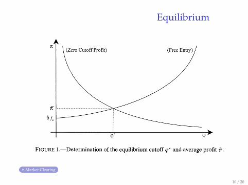
• Thus, there exist a ϕ∗ s.t. π(ϕ∗) = 0→ zero cutoff profit

condition (ZCP).

8 / 20

Firm Entry and Exit• Given µ(ϕ) µ(ϕ) , we can define aggregate productivity

as function of the cutoff:

ϕ(ϕ∗) =

[1

1−G(ϕ∗)

∫ ∞ϕ∗

ϕσ−1g(ϕ)dϕ

] 11−σ

• Moreover, the ZCP implies a relationship between averageprofit and ϕ∗ details :

π(ϕ∗) = 0⇔ r(ϕ∗) = σf ⇔ π = f[(ϕ(ϕ∗)/ϕ∗)σ−1 − 1

](3)

• Free Entry: The net value of entry is equal to the averageprofits minus the entry cost and must be 0 in equilibrium:

ve = (1−G(ϕ∗))π

δ− fe ⇒ π =

δfe1−G(ϕ∗)

(4)

9 / 20

Equilibrium

Market Clearing

10 / 20

Conclusion: Closed Economy

• Welfare per worker: Welfare is given by the real wage:W = P−1 = M

11−σ ρϕ

• Welfare only is higher in a larger country due to productvariety.

• A representative firm model with productivity ϕ andprofit π yields the same results.

• However, the R.F. model cannot induce changes inaggregate productivity due to exposure of trade. Melitzmodel can do it because of the reallocation effect.

11 / 20

Open Economy

• If there is no costs of trade, then the world is just a bigcountry.

• Therefore, we add two types of cost: Per unit iceberg costτ > 1 and a fixed entry cost to sell in a foreign marketfex > 0.

• We assume that there are n symmetric countries and thefirms decide to enter in a foreign market after they knowtheir ϕ.

• For simplicity assume the firm pays an amortizedper-period version of the entry cost: fx = δfex.

12 / 20

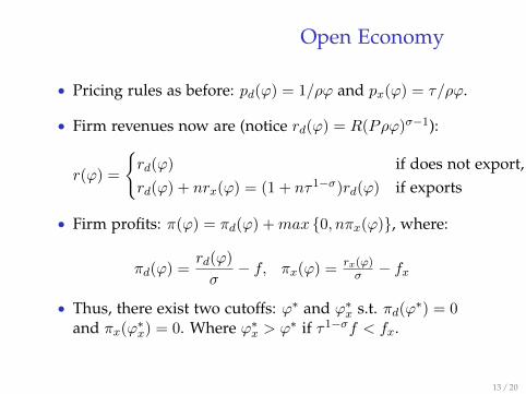
Open Economy

• Pricing rules as before: pd(ϕ) = 1/ρϕ and px(ϕ) = τ/ρϕ.

• Firm revenues now are (notice rd(ϕ) = R(Pρϕ)σ−1):

r(ϕ) =

rd(ϕ) if does not export,rd(ϕ) + nrx(ϕ) = (1 + nτ1−σ)rd(ϕ) if exports

(5)

• Firm profits: π(ϕ) = πd(ϕ) +max 0, nπx(ϕ), where:

πd(ϕ) =rd(ϕ)

σ− f, πx(ϕ) = rx(ϕ)

σ − fx

• Thus, there exist two cutoffs: ϕ∗ and ϕ∗x s.t. πd(ϕ∗) = 0and πx(ϕ∗x) = 0. Where ϕ∗x > ϕ∗ if τ1−σf < fx.

13 / 20

Aggregation• Let M denote the mass of incumbents firms in any

country and define the ex-ante probability of export:px ≡ [1−G(ϕ∗x)]/[1−G(ϕ∗)].

• Mx = pxM then represents the mass of exporting firms.Also, Mt = M + nMx represents the total mass of varietiesavailable.

• Using the same weighted average function defined in (2),the weighted average productivity of all firms:

ϕt =

1

Mt[Mϕ(ϕ∗)σ−1 + nMx(τ−1ϕ(ϕ∗x))σ−1]

1σ−1

(6)

• Again, the aggregate variables: P = M1

1−σt p(ϕt) and

R = Mtrd(ϕt) are easily traceable by ϕt.

14 / 20

Equilibrium

• The free entry condition does not change:π = δfe/[1−G(ϕ∗)].

• However, the ZCP curve shifts up! Notice:

π = πd(ϕ) + pxnπx(ϕx)

= f

[(ϕ(ϕ∗)

ϕ∗

)σ−1

− 1

]+ pxnfx

[(ϕ(ϕ∗x)

ϕ∗x

)σ−1

− 1

]

• The ZCP also implies that: ϕ∗x = ϕ∗τ(fxf

) 1σ−1 .

• Since FE and ZCP defines a unique ϕ∗ and π, once wehave ϕ∗, we can backup ϕ, ϕx, ϕt and all the othervariables.

15 / 20

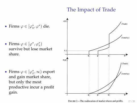
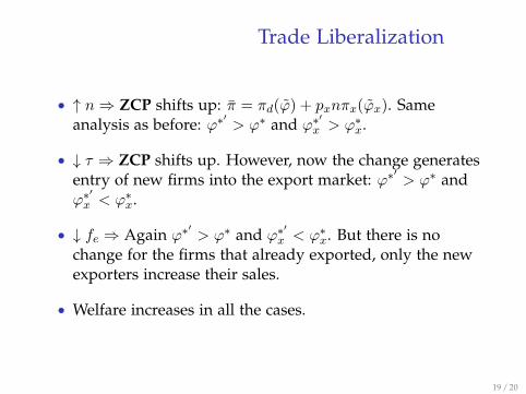
The Impact of Trade

• Using this framework we can compare the SS equilibriumin autarky vs. trade and study the impact of a tradeliberalization: ↑ n, ↓ τ and ↓ fe.

• Autarky vs. trade SS: Since the ZCP shifts up⇒↑ ϕ∗ and↑ π. But the effect is not uniform across firms.

• The open economy decrease the firm’s share of thedomestic market, but the exporters make up for its loss.Market share reallocation→ exporters!

rd(ϕ) < ra(ϕ) < rd(ϕ) + nrx(ϕ) ∀ϕ ≥ ϕ∗ (7)

• Nevertheless, not all the exporters increase their profits.E.g. the firm with ϕ∗x has πx(ϕ∗x) = 0 but πd(ϕ∗x) < πa(ϕ

∗x) .

16 / 20

The Impact of Trade

• Firms ϕ ∈ [ϕ∗a, ϕ∗) die.

• Firms ϕ ∈ [ϕ∗, ϕ∗x)survive but lose marketshare.

• Firms ϕ ∈ [ϕ∗x,∞) exportand gain market share,but only the mostproductive incur a profitgain.

17 / 20

The Impact of Trade• How the reallocation mechanism really works? Because

of the monopolistic competition and the CES utility, firmsdo not really compete against each other.

• However, they compete for the same source of labor! →The increase in labor demand by both the moreproductive firms and the new entrants rises the realwage!

• Remember the aggregate price level: Pa = M1

1−σa /ρϕa and

Pt = M1

1−σt /ρϕt.

• Usually (but not always!) Mt > Ma, but the aggregateproductivity always increase ϕt > ϕa ⇒ P < Pa.

• Even if the number of varieties decrease, welfare alwaysimprove with trade!

18 / 20

Trade Liberalization

• ↑ n⇒ ZCP shifts up: π = πd(ϕ) + pxnπx(ϕx). Sameanalysis as before: ϕ∗

′> ϕ∗ and ϕ∗

′x > ϕ∗x.

• ↓ τ ⇒ ZCP shifts up. However, now the change generatesentry of new firms into the export market: ϕ∗

′> ϕ∗ and

ϕ∗′x < ϕ∗x.

• ↓ fe ⇒ Again ϕ∗′> ϕ∗ and ϕ∗

′x < ϕ∗x. But there is no

change for the firms that already exported, only the newexporters increase their sales.

• Welfare increases in all the cases.

19 / 20

Conclusion

• This paper has described and analyzed a newtransmission channel for the impact of trade on industrystructure and performance.

• It shows that the induced reallocation between differentfirms generate changes in the aggregate environment thatcannot be explained by a representative model.

• The model concludes that the exposure to trade inducereallocation toward the more efficient firms.

• Also, it provides evidence that any trade-enhance policy iswelfare improving.

20 / 20

Appendix

• The conditional distribution of productivity:

µ(ϕ) =

g(ϕ)

1−G(ϕ∗) if ϕ ≥ ϕ∗

0 otherwiseBack (8)

• Average profit and revenues are also tied to ϕ∗:

r = r(ϕ) =

[ϕ(ϕ∗)

ϕ∗

]σ−1

r(ϕ∗), π = π(ϕ) =[ϕ(ϕ∗)ϕ∗

]σ−1r(ϕ∗)σ − f

• Market clearing:

(1−G(ϕ∗))Me = δM, Lp = R−Π, Le = Mefe = Mπ = Π

Back

21 / 20