1 The Impact of Unit Cost Reductions on Gross Profit: Increasing or Decreasing Returns? # Ely Dahan * and V. Srinivasan ** October 10, 2005 * Assistant Professor of Marketing, UCLA Anderson School of Business, 110 Westwood Plaza, B-5.14, Los Angeles, CA 90095-1481 ** Adams Distinguished Professor of Management, Graduate School of Business, Stanford University, Stanford, CA 94305-5015 # Comments on the research from Professors John R. Hauser and Birger Wernerfelt have been most helpful.
Transcript
1
The Impact of Unit Cost Reductions on Gross Profit:
Increasing or Decreasing Returns? #
Ely Dahan* and V. Srinivasan**
October 10, 2005
* Assistant Professor of Marketing, UCLA Anderson School of Business, 110 Westwood Plaza, B-5.14, Los Angeles, CA 90095-1481
** Adams Distinguished Professor of Management, Graduate School of Business, Stanford University, Stanford, CA 94305-5015
# Comments on the research from Professors John R. Hauser and Birger Wernerfelt have been most helpful.
2
Abstract
When asked about the impact of unit manufacturing cost reductions on gross profit, many
managers and academics assume that returns will be diminishing, i.e., that the first cent of unit
cost reduction will generate more incremental gross profit than the last cent of unit cost savings,
consistent with the economic intuition about diminishing returns. (The product’s appeal to the
market is assumed to remain constant.) The present paper shows why gross profits actually
increase in a convex fashion under typical demand assumptions, providing increasing returns
with each additional cent of reduction in unit manufacturing cost. The intuition is that if q units
are sold at the current price, the first cent of unit cost reduction increases the gross profits by q
cents (keeping the price at the current level). But further cost reductions bring about greater
pricing flexibility so that the optimal price decreases, thereby increasing the quantity to q’. Thus,
the last cent of cost reduction produces an incremental profit of q’ cents, where q’ > q. The
convex returns are captured graphically in the “profit saddle,” a simple plot of gross profit as a
function of unit cost and unit price. Decreasing unit costs produce additional returns from
learning curve effects, reduced per unit channel costs, quality improvements, and strategic
considerations. Of course, the fixed investment entailed in reducing unit-manufacturing costs
must be weighed against the returns from doing so, suggesting some optimal level of unit cost
reduction efforts.
Cost reduction has traditionally been the purview of the manufacturing function within
the firm, and has been emphasized in the later phases of the product-process life cycle.
Marketing managers, on the other hand, have focused on generating sales revenues through
pricing, product positioning, promotion, and channel placement. The present paper suggests that
the traditional view be questioned. The marketing function, and new product planning in
particular, may want to consider unit manufacturing cost reduction a potent tool in pricing new
products for marketing success.
1
The Impact of Unit Cost Reductions on Gross Profit: Increasing or Decreasing Returns?
How important are unit manufacturing costs in the design and development of new
products? Many questions arise in determining the optimal cost reduction strategy during new
product development (NPD). For example, should the marketing members of multifunctional
NPD teams be concerned with cost-related decisions even though these issues have traditionally
been the purview of the engineering and manufacturing functions of the firm? Our analysis
shows that, in many cases, marketers should be involved in these decisions from the outset,
consistent with prior research on the need for integration between marketing and manufacturing
during NPD (Wheelwright and Clark 1992, Griffin and Hauser 1996, Kahn 1996). What is the
profit impact of reducing unit manufacturing cost - do incremental cost reductions yield
increasing or diminishing returns? We show that, contrary to the economic intuition of
(Imai 1986, Lee 1996), and the use of postponement (Feitzinger and Lee 1997), modularity
(Baldwin and Clark 2000), and platforms (Meyer and Lehnerd 1997, Ulrich and Eppinger 2000)
2
can all contribute. These approaches complement the direct benefits of investing in unit cost
reduction achieved through clever design.
In this paper, we focus on the nature of the impact of unit cost reduction on gross profits.
Our findings regarding the profit impact of cost reduction efforts run counter to many managers’
and academics’ intuitions. We find that early and effective cost savings efforts may improve the
chances of new product success to a greater extent than is commonly believed, and that the
payoff from unit cost reduction justify significant investment in “smarter” design during the
NPD process (Ulrich and Pearson 1998). In fact, the potential for unit cost reduction may be an
important criterion when selecting a new product concept from amongst competing ideas.
1 Increasing, Linear or Decreasing Returns?
Consider the three possibilities depicted in Figure 1. In all cases, the product in question
is assumed to remain constant in the perceptions of customers. That is, any changes required to
achieve unit cost reductions are assumed to have no effect on the desirability of, willingness-to-
pay for, or probability of purchase of the product at any given price. For instance, cost
reductions may be brought about by design for manufacturability and assembly (Boothroyd,
Dewhurst and Knight 1994) or by sourcing through lower cost suppliers, neither of which alter
the functionality or appearance of the product.
In the lower (dotted) curve, investments in unit cost reduction improve gross profit,
defined as revenues minus variable direct costs, exhibit diminishing returns. That is, the first
cent of unit cost reduction has a greater impact on gross profit than the next cent of cost
reduction. This fits the general economic intuition of diminishing returns. The middle (solid)
line depicts a linear relationship between cost reduction and profit, consistent with the idea that
3
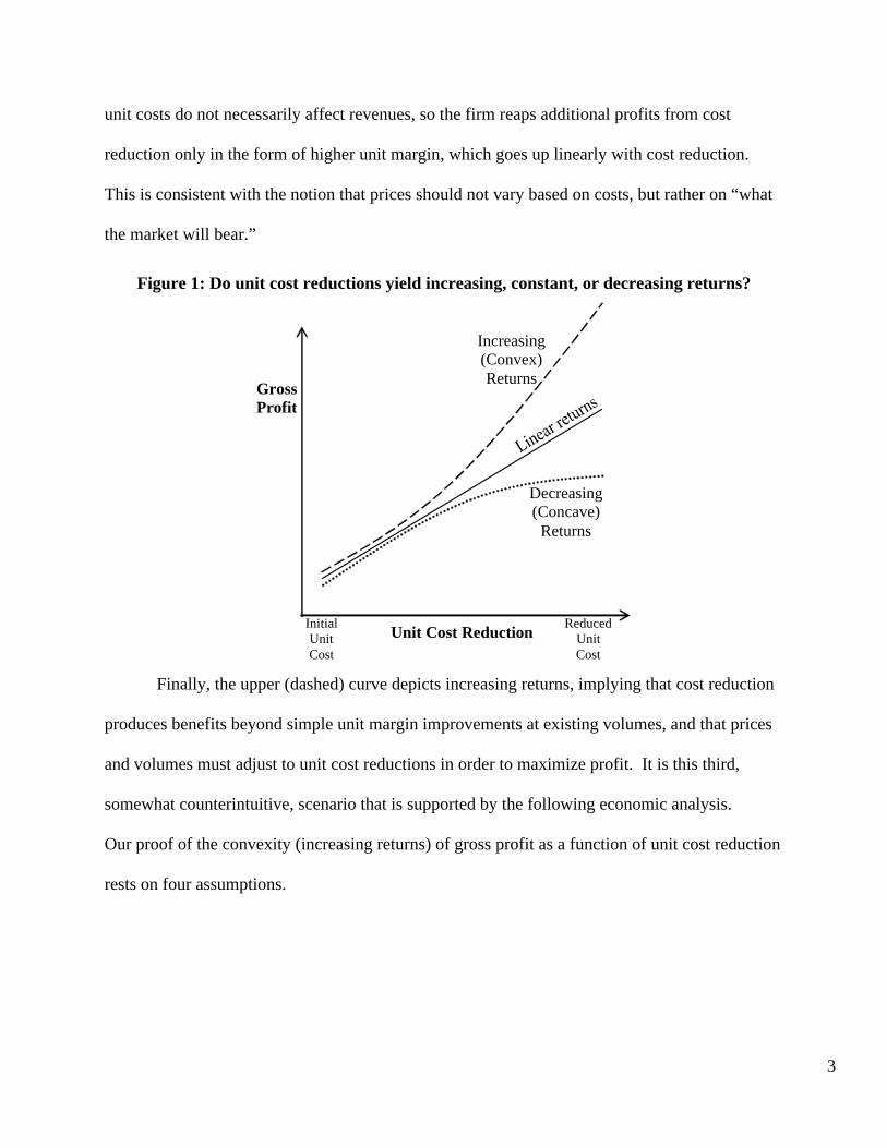
unit costs do not necessarily affect revenues, so the firm reaps additional profits from cost
reduction only in the form of higher unit margin, which goes up linearly with cost reduction.
This is consistent with the notion that prices should not vary based on costs, but rather on “what
the market will bear.”
Figure 1: Do unit cost reductions yield increasing, constant, or decreasing returns?
Unit Cost Reduction
GrossProfit
Initial Unit Cost
Reduced Unit Cost
Decreasing (Concave)
Returns
Increasing (Convex) Returns
Finally, the upper (dashed) curve depicts increasing returns, implying that cost reduction
produces benefits beyond simple unit margin improvements at existing volumes, and that prices
and volumes must adjust to unit cost reductions in order to maximize profit. It is this third,
somewhat counterintuitive, scenario that is supported by the following economic analysis.
Our proof of the convexity (increasing returns) of gross profit as a function of unit cost reduction
rests on four assumptions.
4
Assumptions: • [A1] Proportional Costs: Total Variable Cost (TVC ) is proportional to
quantity (q), so that qcqTVC ⋅=)( , where c denotes the unit (variable) cost.
• [A2] Downward Sloping Demand: The quantity demanded, ( )pq , is a
monotonically decreasing function of price (p): i.e., 0<∂∂
pq p∀ .1
• [A3] Unique Profit-maximizing price: For any given unit cost c, the gross profit function, ( )[ ] )(qTVCpqp −×=π , is strictly quasi-concave and smooth in p, and therefore has a unique, profit-maximizing price, p*, at which point the
function is locally strictly concave, i.e., 02
2<
∂∂
pπ at p*. (cf., Figure 2).
• [A4] Positive Gross Profit: Unit cost, c, is such that the optimal gross profit is strictly positive, i.e., cp >* and ( ) 0* >pq .
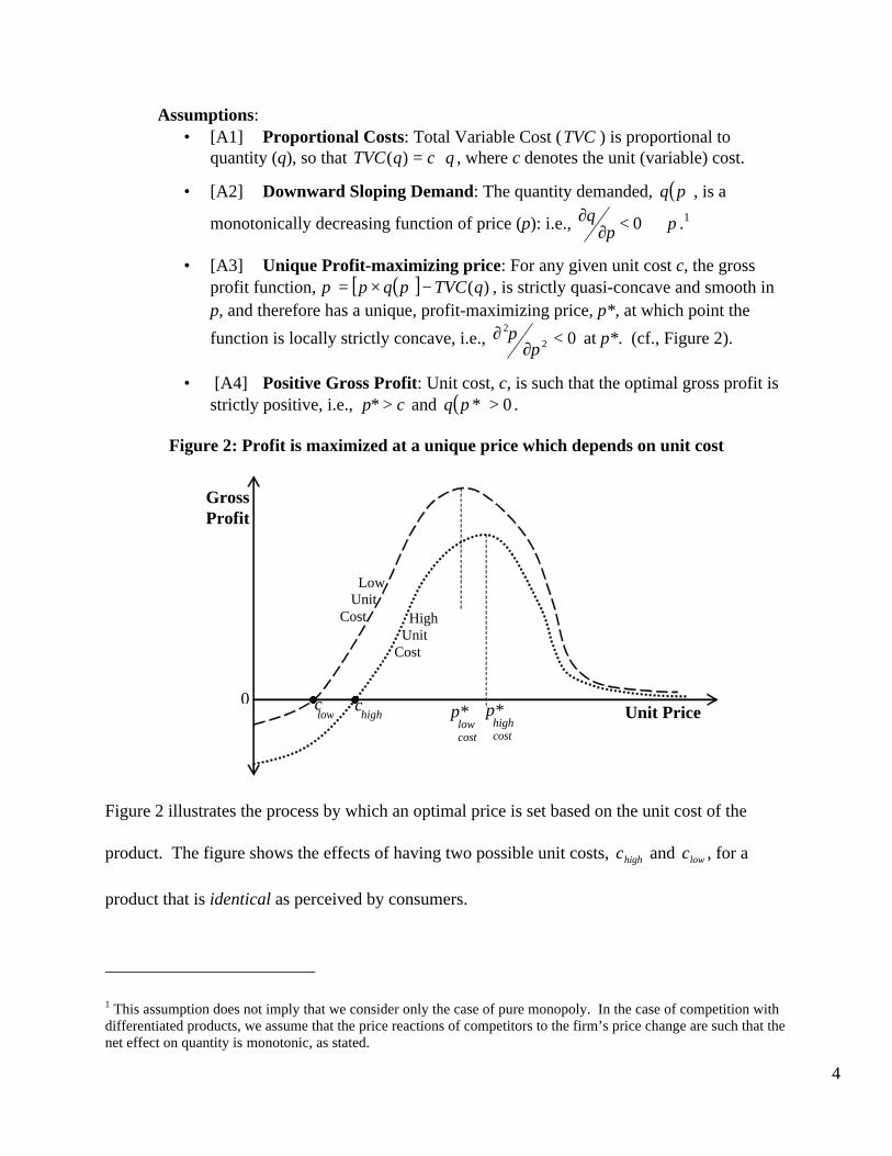
Figure 2: Profit is maximized at a unique price which depends on unit cost
Unit Price
Gross Profit
p* high cost
p* low cost
High Unit Cost
Low Unit Cost
c high
c low
0
Figure 2 illustrates the process by which an optimal price is set based on the unit cost of the
product. The figure shows the effects of having two possible unit costs, highc and lowc , for a
product that is identical as perceived by consumers.
1 This assumption does not imply that we consider only the case of pure monopoly. In the case of competition with differentiated products, we assume that the price reactions of competitors to the firm’s price change are such that the net effect on quantity is monotonic, as stated.
5
Note that gross profits are consistently higher under the lowc regime as would be expected. Note
also that the gross-profit-maximizing price, *p , differs between the two scenarios, and is lower
under the lower-cost regime. For a given unit cost, gross profit declines to the left of *p since
the unit margin is reduced too much, and declines to the right of *p because the sales volume is
reduced too much. Thus, *p represents the point at which the tension between unit gross
margin and total volume is optimized.
Using the above four assumptions, we first show that optimal prices strictly decrease when cost
reductions are achieved. That is, it is optimal to pass on unit cost reductions to consumers to at
least some extent.
Lemma: The optimal price is increasing in cost, i.e., 0* >dcdp .
Proof: The first order condition (FOC) for maximizing the gross profit function shown in
[A3] by setting price optimally is:
(1) ( ) ( )[ ] ( ) 0)( =+
∂∂
−=∂
×−∂=
∂∂
= pqpq
cpp
pqcpp
FOCπ
.
By invoking the Implicit Function Theorem at p*, we see that:
(2) 0*
2
2 >
∂∂
∂∂
=∂
∂∂
∂−=
p
pq
pFOC
cFOC
dcdp
π,
since 0<∂∂
pq by [A2] and 02
2<
∂∂
pπ at p* by [A3]. #
6
Thus when pricing optimally, and given our assumptions, unit cost reductions lead to
strictly lower prices.
Employing the Lemma, we now show that gross profits exhibit increasing returns to cost
reduction. That is, π is convex in c.
Theorem: For any demand function, ( )pq , meeting assumptions [A1] - [A4], the optimal
gross profit, ( ) ( ) ( )***, pqcpcp ×−=π is strictly decreasing and strictly convex in unit cost, c.
That is, ( )
0*,
2
2
>dc
cpd π. Consequently, gross profit returns to unit cost reductions are strictly
increasing and strictly convex.
Proof: Differentiating ( ) ( ) ( )***, pqcpcp ×−=π with respect to c, we have
(3) ( )
dcdp
pcdccpd *
**,
∂∂
+∂∂
=πππ
*)(
**
*)(
pqdc
dpp
pq
−=
⋅∂∂
+−=π
since, by the first order condition (1), 0*
=∂∂pπ
. From the fact that ( ) 0* >pq in [A4] it follows that
profit is strictly decreasing in c, i.e. that profit is strictly increasing with cost reductions. Differentiating
(3) one additional time, we get
(4) ( )
dcdp
pq
dccpd *
**,
2
2
⋅∂∂
−=π
.
Since 0*
<∂∂pq
by [A2] and 0*
>dc
dp by the Lemma,
( )0
*,2
2
>dc
cpd π. #
7
The profit convexity result of Theorem 1 is intuitively explained by Figure 3.
Figure 3: Intuition Underlying Profit Convexity
Unit Cost Reduction
π GrossProfit
Initial Unit Cost
Reduced Unit Cost
clow
chigh
1¢ 1¢
∆π (chigh
)
∆π (clow
)
When unit cost is high before cost reduction efforts, as at chigh
, the optimal price is
correspondingly high (Lemma 1) and the sales volume is therefore low. Thus, reducing a high
unit cost by 1 cent has a small effect on gross profit since the volume being sold is small. When
unit cost is much lower after significant cost reduction, as at clow
, the impact is greater since the
same 1-cent saving applies to a higher volume of units sold since the optimal price will now be
lower. The higher volumes resulting from lower prices may derive from both greater per
customer consumption and a greater number of customers when price is lowered.
Another way of intuitively seeing the convexity result is to observe that if the price is
held constant, gross profit increases linearly with the amount of unit cost reduction. Beyond this
direct benefit of cost reduction, the firm has the flexibility to change its price with any reduction
in cost, and garner an indirect benefit from pricing flexibility. Because this added flexibility, if
optimally exercised, can only increase gross profits over and above the direct linear
improvement, the profit curve will be higher than the tangent to the curve. Because this
8
phenomenon holds true for every value of unit cost, the profit curve is a convex-increasing
function of the amount of unit cost reduction.
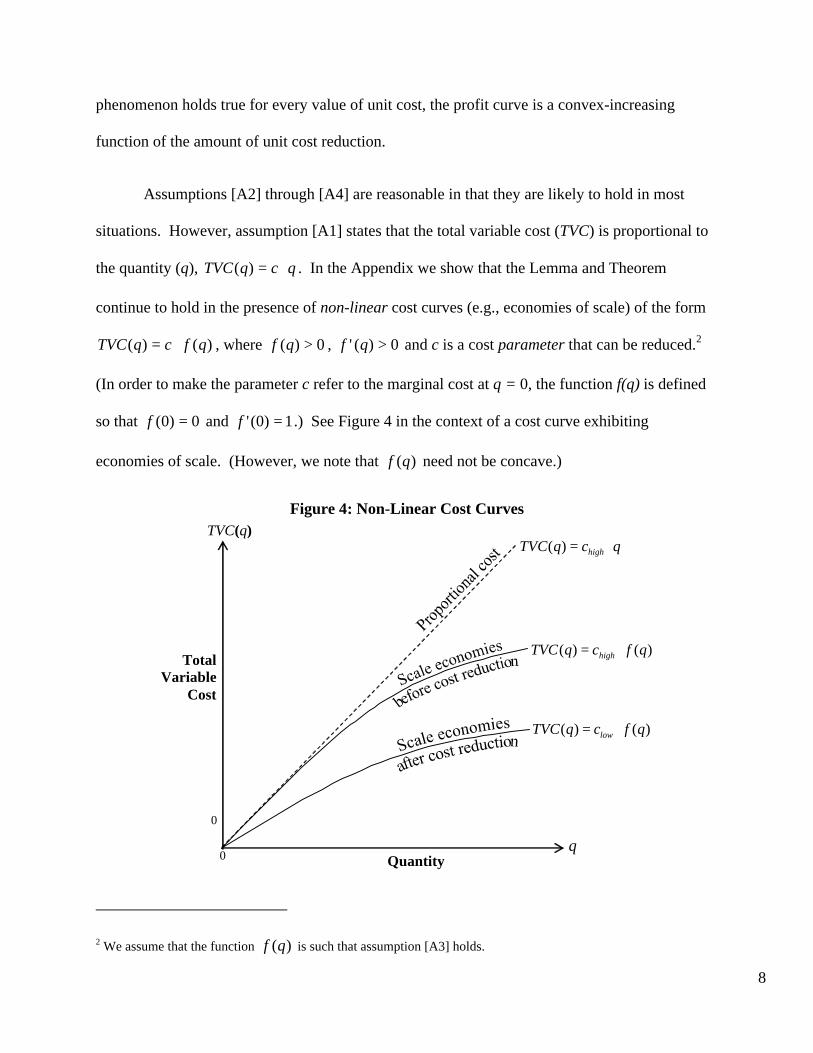
Assumptions [A2] through [A4] are reasonable in that they are likely to hold in most
situations. However, assumption [A1] states that the total variable cost (TVC) is proportional to
the quantity (q), qcqTVC ⋅=)( . In the Appendix we show that the Lemma and Theorem
continue to hold in the presence of non-linear cost curves (e.g., economies of scale) of the form
)()( qfcqTVC ⋅= , where 0)( >qf , 0)(' >qf and c is a cost parameter that can be reduced.2
(In order to make the parameter c refer to the marginal cost at q = 0, the function f(q) is defined
so that 0)0( =f and 1)0(' =f .) See Figure 4 in the context of a cost curve exhibiting
economies of scale. (However, we note that )(qf need not be concave.)
Figure 4: Non-Linear Cost Curves
Quantity
TVC(q)
0 q
Total Variable
Cost
0
qcqTVC high ⋅=)(
)()( qfcqTVC high ⋅=
)()( qfcqTVC low ⋅=
2 We assume that the function )(qf is such that assumption [A3] holds.
9
We now analyze two well-known demand functions, linear demand and constant
elasticity, to illustrate the result.
Example 1: Linear Demand
As a simple example of increasing returns, consider a monopolist facing a demand curve
that is linear in price, 10 <≤ p , with m− being the slope of the demand curve, c being the
constant marginal cost of production ( pc <≤0 , consistent with [A4]), and q the quantity sold.
)1()( :Profit)1( :Function DemandLinear
pmcppmq
−××−=−×=
π
To maximize profit, π, the firm sets its price at 2
1*
+=
cp and realizes profits of
4)1(
)(*2c
mc−
×=π at 2
)1(*
cmq
−×= . Thus, ) inconvex is (i.e.0
2)(
2
2
cm
dccd
ππ
>= . The
second derivative of profit with respect to unit cost is positive for the negatively sloped linear
demand function, thus confirming increasing returns to unit cost reductions. As expected, cost
reductions lead to price reductions
> 0
*dc
dp, and volume increases
< 0
*dc
dq.
Example 2: Constant Elasticity Demand
Similarly, the firm may face demand with constant price elasticity, ε.
ε
ε
π −
−
×−=
=
kpcp
kpq
)( :Profit
, : FunctionDemand
10
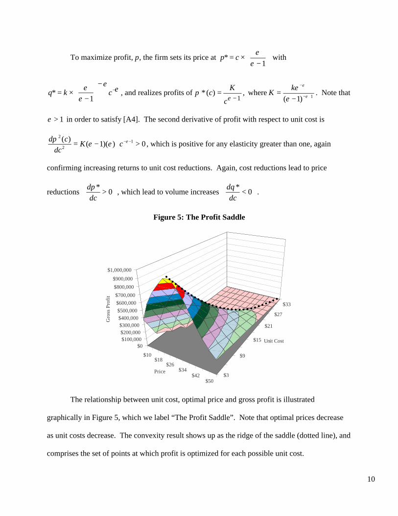
To maximize profit, π, the firm sets its price at
−×=
1*
εε
cp with
εε
εε −
−
−×= ckq
1* , and realizes profits of 1
)(*−
=ε
πc
Kc , 1)1(
where +−
−
−= ε
ε
εεk
K . Note that
1>ε in order to satisfy [A4]. The second derivative of profit with respect to unit cost is
0))(1()( 1
2
2
>⋅−= −−εεεπ
cKdc
cd, which is positive for any elasticity greater than one, again
confirming increasing returns to unit cost reductions. Again, cost reductions lead to price
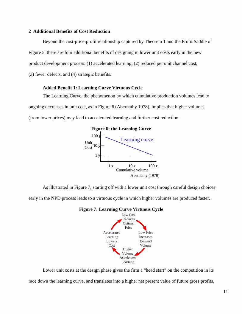
Lower unit costs at the design phase gives the firm a “head start” on the competition in its
race down the learning curve, and translates into a higher net present value of future gross profits.
12
Added Benefit 2: Reduced Unit Channel Cost
Unit cost reduction may reduce unit channel cost by virtue of increased volume.
Wholesalers and retailers, a significant portion of whose costs does not vary directly with
volume, may now amortize their fixed costs over a larger volume of the product, thereby
reducing the per unit cost of distribution. The channel may pass on some of these savings to
consumers, further stimulating sales volume.
Added Benefit 3: Reduction in Defects
Unit cost reduction may, ironically, improve product quality. While intuition might
dictate that lower unit cost implies lower quality, research (Barkan and Hinkley 1994, Mizuno
1988, Taguchi 1987) has demonstrated that cost reduction efforts aimed at reducing the number
of parts and making assembly more efficient also reduce the number of failure modes of the
product, thereby reducing defects. See Figure 8.
Figure 8: Cost Reduction Produces Fewer Defects
Effect of Assembly Efficiency on Quality
1
10
100
1,000
10,000
100,000
0% 10% 20% 30% 40% 50% 60%
Assembly efficiency
Def
ects
mill
ion
parts
From Barkan and Hinkley (1994)
Figure 9 provides data from the leaders in design for manufacturing and assembly,
Boothroyd and Dewhurst, claiming that efforts at reducing unit costs through design for
manufacturing and assembly (DFMA) not only reduce costs through faster assembly and fewer
13
parts, but also reduce assembly defects and the need for service calls, consistent with the
improved quality argument above.
Figure 9: Improvements from Design for Manufacturability and Assembly (DFMA)
From Boothroyd & Dewhurst, www.dfma.com (2004)
They further make the claim that time-to-market may also be halved since the process of
ramping up production becomes much easier when the product design has been simplified for
manufacturability (Smith and Reinertsen 1998). Clearly, if product quality and reliability are
improved and time-to-market is shortened, profits should improve as well.
Added Benefit 4: Keeping Competitors Out of the Market
Unit cost reduction provides potential strategic benefits as depicted in Figure 10, based
on research by Schmidt and Porteus (2001).
Figure 10: The Strategic Benefit of Cost Reduction
0
100
200
300
400
500
InnovativeCompetence, R
Cost Competence, C
Incu
mbe
nt's
expe
cted
pro
fit
ContingentRetrenchment
Domination
ContingentDomination
0%
CH1%
2%3%
1.6 1.4
1.0
1.2
Retrenchment
Ver
tical
clif
f
Incumbent's Expected Profit
0
100
200
300
400
500
InnovativeCompetence, R
Cost Competence, C
Incu
mbe
nt's
expe
cted
pro
fit
ContingentRetrenchment
Domination
ContingentDomination
0%
CH1%
2%3%
1.6 1.4
1.0
1.2
Retrenchment
Ver
tical
clif
f
Incumbent's Expected Profit
From Schmidt and Porteus (2001)
Before DFMA Reductions
14
When the firm establishes itself as the low cost manufacturer, it dissuades competitors
from entering the market, leading to significantly higher profits. The ability to develop and
manufacture products at lower unit costs than competitors, here captured by the cost competence
factor, C, may be as important as the ability to develop more innovative products, captured by R.
By being competent at unit cost reduction, incumbent market leaders are able to keep potential
entrants at bay.
3 Optimal Cost Reduction
Having established the increasing returns to unit cost reduction, one must weigh this
against the “costs of cost reduction,” which take the form of investments that are independent of
the volume of products sold. These investments take many forms, each of which may contribute
to the overall reduction in unit cost. For example, design for manufacturing and assembly
(DFMA), process automation, operational efficiency and variance reduction, and improved
purchasing have cumulative effects on unit cost reduction. Analytically, these potential
investments can be summarized by a function as depicted by the dashed curve in Figure 11.
Figure 11: Profit is Optimized When Marginal Gross Profit Equals Marginal Investment
Dollars
Unit Cost Reduction
Parallel slopes (Marginal gross profit
equals Marginal investment)
OptimalInvestment
in Cost Reduction
Optimal Cost Reduction
15
The dashed curve relates the level of investment in cost reduction efforts, amortized to coincide
with the time frame used in the unit gross profit contribution analysis, to their effect on unit
costs. We assume that such investments are made optimally to achieve the greatest amount of
cost reduction for the least amount of investment, making the function convex (i.e. earlier
investments have higher payoffs). We further assume that the degree of convexity of the
investment function is greater than that of the gross profit returns to unit cost reduction, the
dotted line in Figure 11.
Under the above conditions, there exists a unique level of investment in unit cost
reduction at which net profits, that is gross profit contribution minus the (amortized) investment
in cost reduction, is maximized. This occurs at the point where the marginal benefit of reducing
the unit cost is equal to the marginal (amortized) investment required to achieve that unit cost.
Of course, a richer analysis factoring in the added benefits of unit cost reduction and more richly
detailed investment function might produce a less “clean” result, but the analysis would proceed
along much the same lines.
In summary, unit cost reduction has been shown to have increasing returns due to the
attendant price reductions and increased volume, and additional benefits due to the virtuous cycle
of the learning curve, reduced channel costs, potential quality improvements, and strategic
effects. These benefits should be carefully evaluated and traded off against the investment
required to achieve unit cost reductions. While unit cost reduction efforts during NPD have
traditionally been the purview of manufacturing personnel in the firm, these analyses suggest that
their impact offers a pricing advantage when developing new products for future marketing
success.
16
Appendix
Lemma (Non-linear Cost function): Given the Total Variable Cost Function, )()( qfcqTVC ⋅= ,
with 0)( >qf and 0)(' >qf , the optimal price p* is increasing in the cost parameter c, i.e., 0* >dcdp .
Proof: The gross profit ( ))()( pqfcpqp ⋅−⋅=π . The first order condition (FOC) for maximizing π
by setting price optimally is:
0)(')(')()(' =×−+=∂∂
= pqqfcpqpqpp
FOCπ
.
By invoking the Implicit Function Theorem at p*, we see that:
0)(')('*
2
2 >
∂∂
=∂
∂∂
∂−=
p
pqqf
pFOC
cFOC
dcdp
π,
since 0)(' >qf , 0)(' <pq by Assumption [A2], and 02
2<
∂∂
pπ at p* by [A3]. Thus 0* >dc
dp . #
Theorem (Non-linear Cost function): Given the Total Variable Cost Function, )()( qfcqTVC ⋅= ,
with 0)( >qf and 0)(' >qf , the profit function is convex in the cost parameter c, i.e., ( )
0*,
2
2
>dc
cpd π.
Proof: ( )*)(*)(*)*,( pqfcpqpcp ⋅−⋅=π .
( )cdc
dppcdc
cpd∂∂
=∂∂
+∂∂
=ππππ *
**,
, because 0*
=∂∂pπ
by the FOC.
[ ] 0*)( <−= pqf
[ ]dc
dppqpqf
dccpd *
*)('*)(')*,(
2
2
−=π
Because 0)(' >qf , 0)(' <pq (Assumption [A2]), and, 0* >dcdp (Lemma), it follows that
( )0
*,2
2
>dc
cpd π, i.e., that π is convex in c. #
17
References Abernathy, William J., (1978), The Productivity Dilemma. Baltimore, MD: Johns Hopkins Press.
Altschuler, Genrich, (1996), And Suddenly the Inventor Appeared. Worcester, MA: Technical Innovation Center, Inc.
Baldwin, Carliss Y. and Kim B. Clark (2000). Design Rules: The Power of Modularity. Cambridge, MA: MIT Press.
Barkan, Philip and Martin Hinckley (1994). “Benefits and Limitations of Structured Methodologies in Product Design,” in Management of Design: Engineering and Management Perspectives, Sriram Dasu and Charles Eastman (eds.), Boston: Kluwer Academic, 163-177.
Boothroyd, Geoffrey, Peter Dewhurst, and Winston Knight (1994), Product Design for Manufacturability and Assembly. New York, NY: Marcel Dekker.
Chew, Bruce and Robin Cooper (1996). “Control Tomorrow's Costs Through Today's Designs,” Harvard Business Review, (January), 88-97.
Dahan, Ely and Haim Mendelson (2001), “An Extreme Value Model of Concept Testing,” Management Science, 47 (January), 102-116.
______ and V. Srinivasan (2000), “The Predictive Power of Internet-Based Product Concept Testing Using Visual Depiction and Animation,” Journal of Product Innovation Management, 17, 2 (March), 99-109.
Feitzinger, Edward and Hau L. Lee (1997), “Mass Customization at Hewlett-Packard: The Power of Postponement.” Harvard Business Review, (January-February), 116-121.
Griffin, Abbie and John R. Hauser (1996), “Integrating Mechanisms for Marketing and R&D," Journal of Product Innovation Management, 13, 3 (May), 191-215.
Imai, Masaaki (1986), Kaizen: The Key to Japan’s Competitive Success. New York, NY: Random House.
Kahn, Kenneth B. (1996), “Interdepartmental Integration: A Definition with Implications for Product Development Performance,” Journal of Product Innovation Management, 13, 2 (March), 137-151.
Lee, Hau L., (1996), “Effective Inventory and Service Management Through Product and Process Redesign,” Operations Research, 44, 1 (January-February), 151-159.
Meyer, Mark and Alvin Lehnerd (1997), The Power of Product Platforms. New York, NY: The Free Press.
Mizuno, S. (1988), Management for Quality Improvement. Cambridge, MA: Productivity Press, 116-128.
Pugh, Stuart. (1996), Creating Innovative Products Using Total Design. Reading, MA: Addison-Wesley.
Schmidt, Glen L. and Evan Porteus (2001), “Sustaining Technology Leadership Can Require Both Cost Competence and Innovative Competence”, Manufacturing and Service Operations Management, 2, 1 (Winter), 1-18.
Smith, Preston G. and Donald G. Reinertsen (1998), Developing Products in Half the Time, 2E. New York, NY: John Wiley & Sons, Inc.
Srinivasan, V., William S. Lovejoy, and David Beach (1997), “Integrated Product Design for Marketability and Manufacturing,” Journal of Marketing Research, 34 (February), 154-163.
Taguchi, Genichi (1987), Introduction to Quality Engineering: Designing Quality into Products and Processes. White Plains, NY: Kraus International Publications.
Ulrich, Karl T. and Scott Pearson (1998), “Assessing the Importance of Design Through Product Archaeology,” Management Science, 44, 3 (March), 352-369.
______ and Steven D. Eppinger (2000), Product Design and Development, 2E. New York, NY: McGraw-Hill, Inc.
Urban, Glen L. and John R. Hauser (1993), Design and Marketing of New Products, 2E. Englewood Cliffs, NJ: Prentice Hall.
Ward, Allen C., Jeffrey K. Liker, John J. Cristiano, Durward K. Sobek II (1995), “The Second Toyota Paradox: How Delaying Decisions Can Make Better Cars Faster,” Sloan Management Review, 36, 3 (Spring), 43-61.
Wheelwright, Steven C. and Kim B. Clark (1992), Revolutionizing Product Development. New York, NY: The Free Press.