The Implications of Cash Flow Forecasts for Investors’ Pricing and Managers’ Reporting of Earnings Andrew C. Call* University of Washington January 24, 2007 Abstract: I examine the role of analysts’ cash flow forecasts on both investors’ pricing and managers’ reporting of earnings. I find that when setting stock prices, investors place more (less) weight on the cash (accrual) component of earnings for firms with a cash flow forecast, and that this weighting is a function of firm-specific factors predicted to affect the usefulness of the underlying cash flow information. Additionally, even when cash flow information is expected to be particularly useful to investors, only in the presence of a cash flow forecast do investors increase the weight they place on the cash component of earnings. I also find that for firms with a cash flow forecast, the cash (accrual) component of earnings is more (less) predictive of future firm prospects, consistent with analysts successfully choosing firms for which to issue a cash flow forecast. Lastly, I document that managers are more likely to opportunistically boost operating cash flows if the firm has a cash flow forecast, suggesting that the nature of the capital market pressure affects the mechanism through which earnings are managed. _________________________ *I am grateful for the support and guidance of my dissertation committee: Terry Shevlin (chair), Yu-chin Chen, Dawn Matsumoto, Terry Mitchell, Shiva Rajgopal, and Eugene Silberberg. I also thank Bob Bowen, Shuping Chen, Max Hewitt, Steve Stubben, Ryan Wilson and workshop participants at the University of Washington for their valuable comments.
Transcript
The Implications of Cash Flow Forecasts for Investors’ Pricing and Managers’ Reporting of Earnings
Andrew C. Call*University of Washington
January 24, 2007
Abstract: I examine the role of analysts’ cash flow forecasts on both investors’ pricing and managers’ reporting of earnings. I find that when setting stock prices, investors place more (less) weight on the cash (accrual) component of earnings for firms with a cash flow forecast, and that this weighting is a function of firm-specific factors predicted to affect the usefulness of the underlying cash flow information. Additionally, even when cash flow information is expected to be particularly useful to investors, only in the presence of a cash flow forecast do investors increase the weight they place on the cash component of earnings. I also find that for firms with a cash flow forecast, the cash (accrual) component of earnings is more (less) predictive of future firm prospects, consistent with analysts successfully choosing firms for which to issue a cash flow forecast. Lastly, I document that managers are more likely to opportunistically boost operating cash flows if the firm has a cash flow forecast, suggesting that the nature of the capital market pressure affects the mechanism through which earnings are managed.
_________________________
*I am grateful for the support and guidance of my dissertation committee: Terry Shevlin (chair), Yu-chin Chen, Dawn Matsumoto, Terry Mitchell, Shiva Rajgopal, and Eugene Silberberg. I also thank Bob Bowen, Shuping Chen, Max Hewitt, Steve Stubben, Ryan Wilson and workshop participants at the University of Washington for their valuable comments.
1
The Implications of Cash Flow Forecasts for Investors’ Pricing and Managers’ Reporting of Earnings
1. Introduction
One of the primary inputs to firm value is earnings (Ohlson 1995). Earnings represents
the most widely-used measure of firm performance, and is the sum of operating cash flows and
accounting accruals. In this paper, I study the effect of analysts’ cash flow forecasts on the
weight investors place on the accrual and cash components of earnings when valuing firms.
Specifically, I examine whether the mere presence of a cash flow forecast impacts investors’
pricing decisions, and whether the impact of a cash flow forecast is independent of the effect of
firm-specific factors that likely affect the usefulness of the underlying cash flow information. I
also explore the impact of analysts’ cash flow forecasts on managers’ reporting of cash flow
information.1
Financial analysts play an important role in collecting and disseminating information
about the future prospects of the firms they follow. In recent years, analysts’ forecasts of cash
from operations have become increasingly common (from 4% of firms with an earnings forecast
in 1993 to 54% in 2005). Cash flow forecasts provide an additional source of information about
the cash component of earnings, and the presence of a cash flow forecast can be viewed by
investors as a signal of the importance of the firm’s underlying cash flow information.
Consistent with this notion, I find that investors incorporate more (less) cash flow (accrual)
information into stock prices for firms with a cash flow forecast. Additionally, investors
decrease the weight they place on the accrual component of earnings immediately following
analysts’ initial cash flow forecast, suggesting that the presence of a cash flow forecast changes
investors’ perceptions of the relative importance of these two earnings components. 1 Throughout this paper, all references to “cash” or “cash flow information” refer to operating cash flows.
2
I also argue that firm-specific earnings and operating characteristics are relevant to the
weight investors place on accrual and cash flow information. Consistent with prior research
(Dechow 1994; DeFond and Hung 2003), I contend that in certain settings, cash flow
information is more useful in assessing firm performance than in other settings. For example, I
conjecture that cash flow information is more useful to investors when earnings are less
informative (e.g., when earnings contain a large accrual component, when accounting method
choices are heterogeneous relative to peer firms, and when earnings are volatile). I also contend
that cash flow information is more useful to investors for firms with short trade cycles and when
the firm relies on internally-generated cash flows (e.g., capital intensive firms and firms in
financial distress). I examine whether investors place more (less) weight on the cash (accrual)
component of earnings when assessing firm value for firms exhibiting these characteristics.
In assessing the usefulness of the underlying cash flow information, I perform factor
analysis to combine these six cross-sectional variables (absolute value of accruals, earnings
volatility, heterogeneity of accounting choice, trade cycle, capital intensity, and financial
distress) into a parsimonious measure that captures the overall usefulness of the firm’s operating
cash flows. I refer to this composite measure as ‘CFUSE’ as it captures the usefulness of the
underlying cash flow information. I find that investors incorporate more (less) cash flow
(accrual) information into stock prices for firms with a high CFUSE score, consistent with the
notion that investors assess the valuation relevance of accrual and cash flow information based
on firm-specific earnings and operating characteristics. Moreover, I find that the usefulness of
the underlying cash flow information (CFUSE) strengthens the effect of a cash flow forecast on
investors’ weighting of the earnings components.
3
Furthermore, the effect of a cash flow forecast on investors’ pricing of earnings is
incremental to the effect of the usefulness of the underlying cash flow information. This finding
has important implications for the role of analysts in the capital markets. It is widely known that
investors incorporate analysts’ forecasted information into their valuation judgments (Skinner
and Sloan 2002). However, this study further suggests that investors view analysts’ decisions to
issue cash flow forecasts as a credible signal of the relative valuation usefulness of the firm’s
accrual and cash components of earnings.
I also examine whether investors’ differential weighting of the cash and accrual
components of earnings is consistent with the ability of these earnings components to predict
future cash flows. Given that stock prices reflect the present value of expected future cash flows,
investors should put more (less) weight on the cash (accrual) component of earnings only when
such information is more (less) useful in predicting future cash flows. I find that current cash
flows are more useful in predicting future cash flows for firms with cash flow forecasts. I also
find that current cash flows (accruals) are more (less) useful in predicting future cash flows for
firms with a high CFUSE score. These results imply that investors are justified in increasing
(decreasing) the weight they place on the cash (accrual) component of earnings in the presence
of a cash flow forecast or when firm characteristics indicate the firm’s cash flow information is
relatively useful.
Finally, I examine the effect of cash flow forecasts on managers’ financial reporting
decisions. Relying on the framework outlined in Dechow et al. (1998) to model normal levels of
operating cash flows, I find that firms with cash flow forecasts report abnormally high operating
cash flows. To further investigate this issue, I find that among firms with a cash flow forecast,
firms that meet or barely beat analysts’ earnings forecasts are more likely to have abnormally
4
high cash from operations than are firms that either miss analysts’ earnings forecasts or beat
analysts’ earnings forecasts by a wide margin. Furthermore, relative to other firms that meet or
barely beat analysts’ earnings forecasts, firms with a cash flow forecast that meet or barely beat
analysts’ earnings forecasts are more likely to do so with abnormally high operating cash flows.
These findings are consistent with the notion that managers of firms with cash flow forecasts
respond to heightened investor and analyst attention to cash flow information by artificially
boosting cash from operations.
This paper adds to the accounting literature in several ways. First, I add to the literature
that examines the role of financial analysts in the capital markets. Numerous studies have
examined how investors incorporate analysts’ forecasts into stock prices (Bartov et al. 2002;
Skinner and Sloan 2002). These studies typically identify a sample of firms, all of which have
an analyst forecast, and examine the impact of these forecasts on stock prices. I, however,
examine a different aspect in which analyst behavior influences investors’ use of accounting
information. Rather than focusing on how investors use analysts’ forecasts themselves, I
examine the impact of analysts’ decisions to issue a forecast on investors’ pricing decisions and
find that analysts’ coverage decisions have valuation implications.
Second, I show that the cash (accrual) component of earnings is more (less) informative
about future cash flows for firms with a cash flow forecast. This finding suggests that analysts
are successfully able to identify firms with highly predictive cash flow information, and that they
issue cash flow forecasts for these firms. Additionally, it suggests investors are successfully able
to incorporate to a greater (lesser) degree accounting information that has more (less) association
with future firm prospects.
5
Finally, I add to the earnings management literature by showing that analysts’ decisions
to issue cash flow forecasts affect managers’ reporting of operating cash flows. I find that
managers of firms with a cash flow forecast are more likely to artificially boost cash from
operations, particularly to avoid reporting a negative earnings surprise. Given that the cash flow
information of firms with a cash flow forecast is under increased scrutiny from investors and
analysts, these results suggest that cash flow forecasts impose market pressures on managers, and
that these pressures impact managers’ decision to artificially boost operating cash flows.
Additionally, this finding suggests that the nature of the capital market pressure can impact the
mechanism through which earnings are managed.
The remainder of this paper is organized as follows. In Section 2, I develop and motivate
the hypotheses. I describe the sample and define the variables of interest in Section 3. Section 4
reports the results related to the pricing of the earnings components and in Section 5 I present my
findings related to managers’ reporting of abnormal operating cash flows. Section 6 concludes.
2. Hypotheses Development
Prior research has examined both the relative and incremental information content of
earnings (accrual) and cash flow information (Biddle et al. 1995; Dechow 1994; Bowen et al.
1987). While earnings are generally considered to be relatively more informative than operating
cash flows, cash flow information contributes information incrementally useful to investors in
valuing firms. However, the degree to which investors incorporate cash flow (accrual)
information into stock prices is not likely to be a cross-sectional constant. I examine situations
in which cash flow (accrual) information is expected to receive relatively more (less) weight by
capital market participants in security valuation.
6
Specifically, I outline two factors that I predict will impact the degree to which investors
incorporate cash flow and accrual information into stock prices. In Section 2.1, I examine the
role that analysts’ cash flow forecasts play in the degree to which investors incorporate the
earnings components into prices. In Section 2.2, I outline earnings and operating characteristics
that likely impact investors’ use of the earnings components. I discuss the correlation between
cash flow forecasts and these earnings and operating characteristics in Section 2.3. In Section
2.4, I outline in more detail my tests concerning the joint impact of cash flow forecasts and firm-
specific characteristics on investor behavior. Finally, in Section 2.5, I discuss the effect of cash
flow forecasts on managers’ propensity to manage earnings by artificially inflating operating
cash flows.
2.1 Cash flow forecasts as a signal
There are several reasons why investors might place more (less) weight on cash flow
(accrual) information in the presence of a cash flow forecast. First, issuing a cash flow forecast
requires additional effort on the part of the analyst, over and above the effort required to issue an
earnings forecast. Given that analysts are among the most sophisticated participants in the
capital markets, investors may view this additional effort and attention to operating cash flows as
a credible signal of the usefulness and importance of the underlying cash flow information.
Accordingly, I expect investors to increase (decrease) the weight they place on the cash (accrual)
component of earnings when analysts issue a cash flow forecast.
Second, analysts’ forecasts provide investors with a richer information set with which to
evaluate firms. If investors have more information with which to estimate, evaluate, and forecast
the cash component of earnings, it is natural that this component of earnings would receive
relatively more weight in firm valuation. As a result, I make the following prediction:
7
H1: Investors place relatively more (less) weight on the cash (accrual) component of earnings when analysts issue a cash flow forecast.
2.2 Earnings and operating characteristics
2.2.1 Earnings characteristics
Magnitude of accruals
Accruals are one of the key outputs of the accounting process. Accrual-based earnings
are generally superior to cash-based earnings because accruals smooth out the timing and
matching problems inherent with cash flows (Dechow 1994). However, there are at least two
drawbacks to accrual-based earnings. First, even in the absence of earnings management,
accruals are estimated with error. These estimation errors add noise to earnings and garble the
information that would otherwise be communicated by earnings (Dechow and Dichev 2002).
The larger the accrual component of earnings, the greater the potential for estimation errors that
distort the information in earnings. Second, accruals are subject to managerial manipulation.
Because of capital market, compensation, and other contracting incentives, managers may distort
accrual numbers in order to report a more favorable earnings figure (Teoh et al. 1998; Healy
1985; DeFond and Jiambalvo 1994). Such managerial intervention, however, results in further
estimation errors that potentially mask the information otherwise inherent in earnings. As a
result, investors have the incentive to decrease (increase) the weight they place on the accrual
(cash) component of earnings when accruals are large in magnitude. Furthermore, large accruals
result in a wide gap between reported earnings and reported operating cash flows. Such a gap
likely gives investors pause and encourages them to interpret earnings with caution.
Earnings volatility
Volatile earnings are generally perceived as being of low quality and diminished
usefulness to investors (Chaney and Lewis 1995; Tucker and Zarowin 2006). Highly volatile
8
earnings are difficult to forecast, as they are less persistent and less predictable. As a result,
investors’ forecasts of earnings are less accurate when earnings are volatile.
In the presence of earnings volatility, investors are likely to rely on more predictable
information sources when interpreting earnings in order to better assess firm value, more
precisely evaluate current firm performance, and more accurately predict future firm
performance. I posit that when earnings (accruals) are volatile, relative to the volatility of cash
from operations, investors will assign more (less) weight the cash (accrual) component of
earnings when valuing the firm.
Accounting choice heterogeneity
When assessing firm performance, capital market participants frequently assess not only
the level of performance reported by the firm, but also the relative performance of the firm when
compared to a set of peer firms (Christie and Zimmerman 1994). Peer-to-peer comparisons are
helpful because they remove the effect of any industry-wide shocks on firm performance.
Peer comparisons are relatively common in the capital markets. For example, Standard
& Poor’s makes peer-to-peer comparisons when assigning credit ratings. Standard & Poor’s
states that it evaluates a “company’s performance and position relative to…its peer group.”
They further explain that their process is “one of comparisons, so it is important to have a
common frame of reference” (Standard & Poor’s 2002). Peer firms are frequently defined as
those firms within the same industry.
Part of the flexibility afforded by GAAP allows managers the ability to choose among
various accounting methods. When managers report earnings reflecting the use of different
accounting methods, it becomes more difficult for investors to compare earnings across firms.
As a result, investors have the incentive to place greater emphasis on the cash component of
9
earnings, as the cash component of earnings is less affected by these accounting choices than is
the accrual component of earnings.
2.2.2 Operating characteristics
Trade cycle
Dechow (1994) finds that operating cash flows is a relatively poor measure of firm
performance for firms with long trade cycles. The intuition is that long trade cycles are
consistent with lumpy cash flows, which impair the ability of cash from operations to accurately
measure economic performance. Earnings, on the other hand, incorporate working capital
accruals which help smooth the lumpiness and produce a more informative measure of
performance. I therefore expect the weight investors place on the cash (accrual) component of
earnings to decrease (increase) with the length of the firm’s trade cycle.
Capital intensity
Capital intensive firms are those with a high degree of fixed assets in place. For these
firms, maintaining and replacing these fixed assets is critical to remaining a profitable enterprise.
However, considerable amounts of cash are required for routine maintenance and replacement of
fixed assets. While capital intensive firms can turn to various sources for the necessary cash
(operating, investing, financing), evidence of internally-generated cash flows (operating cash
flows) is likely to be of interest to investors. This notion is consistent with Standard & Poor’s
increased emphasis on cash flow information when evaluating the credit worthiness of capital
intensive firms (Standard & Poor’s 2002). While external sources of cash can also serve as a
short-term supply of cash for capital intensive firms, investors are likely to demand evidence that
these firms are able to meet their cash flow obligations through internal sources. Accordingly,
10
the cash (accrual) component of earnings is more (less) relevant to firm value for capital-
intensive firms.
Financial health
Firms in financial distress are under particular pressure to demonstrate solvency and the
ability to continue as a going concern. For these firms, the ability to generate operating cash
flows is of particular importance. Ohlson (1980) finds that internally-generated cash flows are
significantly negative in the year prior to bankruptcy. Beaver (1966) reports similar results in the
years preceding “failure.” In general, firms that are unable to generate positive operating cash
flows will not be able to continue as a going concern. For firms in financial distress, the ability
to demonstrate positive operating cash flows is of principal importance.
Furthermore, financially-distressed firms are less able to generate cash flows from
external sources. Not only is the cost of equity higher for financially-distressed firms, but also
there are fewer sources of external capital. This difficulty in raising external capital further
increases the reliance on internal sources of cash flows for financially-distressed firms.
Therefore, for firms in financial distress, I expect investors to assign more (less) weight to the
cash (accrual) component of earnings.
2.2.3 Factor analysis
I perform factor analysis to combine each of the above cross-sectional variables into one
composite measure of the usefulness of cash from operations. Combining these variables into
one summary variable is important for two reasons. First, in the empirical tests that follow,
using a single, parsimonious measure to assess the usefulness of cash flow information simplifies
the research agenda.
11
Second, while each of the above cross-sectional variables is expected to be related to the
usefulness of cash flow information (for the reasons outlined above), they likely capture other
aspects of the firm that are unrelated to the usefulness of cash flow information. For example, as
discussed above, large accruals increase the likelihood of estimation errors being incorporated
into earnings. The result is a relatively less (more) informative accrual (cash) component of
earnings. However, a large accrual component is also consistent with accruals reducing the
timing and matching problems inherent in cash flows, resulting in a superior measure of firm
performance (Dechow 1994). While large accruals can, in one respect, impair the usefulness of
earnings, they can, in another respect, enhance the usefulness of earnings.
As a result, I use factor analysis to capture the common component of each variable.
While each variable likely reflects various aspects of the firm, the common portion of each
variable is the portion that reflects the usefulness of cash flow information. Factor analysis
captures this common portion. The resulting factor score, CFUSE, provides a more reliable
measure of the usefulness of cash flow information than any one variable, and consequently,
increases the power of the empirical tests that follow. This leads to my second hypothesis:
H2: Investors place relatively more (less) weight on the cash (accrual) component of earnings when the underlying cash flow information is relatively useful.
2.3 Relation between the presence of a cash flow forecast and useful cash flow information
DeFond and Hung (2003) examine the determinants of cash flow forecasts, and argue that
analysts respond to investor demand by issuing cash flow forecasts when such forecasts would
be useful to investors. They identify a set of variables predicted to drive investor demand for
cash flow information (some of the variables used above) and find that analysts are more likely
to issue cash flow forecasts for firms exhibiting these characteristics.
12
I, however, show that the set of firms that have a cash flow forecast is not the same as the
set of firms with useful cash flow information. Specifically, more than one-third of all firms
with a cash flow forecast have a factor score that is lower than the median factor score.
Furthermore, two-thirds of all firms with a factor score above the median do not have a cash flow
forecast. These results suggest that the presence of a cash flow forecast does not fully capture
the usefulness of cash flow information.
The fact that the presence of a cash flow forecast is not the same as a high factor score is
not surprising for at least two reasons. First, if the firms with useful cash flow information were
the same firms that had a cash flow forecast, it would imply that (a) analysts are perfectly able to
identify investor demand for cash flow information, and (b) analysts are able to perfectly meet
such demand. This is an unlikely proposition.
Second, analysts’ decision to issue cash flow forecasts is not driven entirely by investors’
demand for such information. Ertimur and Stubben (2006) model analysts’ willingness to
provide cash flow forecasts and find that the presence of a cash flow forecast is at least partially
driven by analyst/brokerage characteristics. They find that analysts who issue inaccurate and/or
frequent earnings forecasts are more likely to issue cash flow forecasts. They also find that
analysts from large brokerages are more likely to issue cash flow forecasts, likely due to the
additional external resources available to analysts at large brokerages (Clement 1999). These
determinants of a cash flow forecast are independent of the valuation usefulness of the
underlying cash flow information, and support the idea that some firms with (without) relatively
useful cash flow information would not (would) have a cash flow forecast.
In summary, there are a large number of firms for which investors would demand cash
flow forecasts that do not actually have a cash flow forecast. Similarly, some firms have a cash
13
flow forecast even though the underlying firm characteristics suggest investors do not demand
one. I report evidence consistent with this notion in Section 4.
2.4 Cash flow forecasts and firm-specific characteristics – incremental and conditional analyses
In addition to individually examining the effect of cash flow forecasts and CFUSE on
investors’ pricing of the earnings components, I also examine how these two factors jointly
determine investors’ pricing behavior. That is, I examine whether cash flow forecasts have an
effect on investors’ pricing of earnings incremental to the effect of CFUSE, and vice versa. This
analysis addresses the question of whether investors’ pricing decisions are based on (a) analyst
behavior, (b) the underlying cash flow information, or (c) both.
I also examine the interaction between these two phenomena. Specifically, I test whether
the impact of a cash flow forecast on investors’ pricing decisions is conditional upon the firm’s
underlying cash flow information. Similarly, I test whether the impact of the usefulness of the
firm’s underlying cash flow information (CFUSE) is conditional upon whether analysts have
issued a cash flow forecast.
How investors jointly process (a) the usefulness of cash flow information and (b) the
presence (or absence) of a cash flow forecast is ultimately an empirical question. As such, I do
not make formal predictions concerning these tests.
2.5 Managers’ reporting decisions
The notion that managers have incentives to manage earnings to reach certain targets has
been widely established. Managers who fail to meet these targets can suffer negative
consequences, including a drop in the firm’s stock price (Bartov et al. 2002), lower
compensation (Matsunaga and Park 2001), and potential termination.
14
When managers want to boost earnings to meet certain targets, they can do so either by
manipulating accruals or by manipulating cash from operations. To boost accruals, managers
can alter the assumptions used to calculate depreciation expense, change estimates of
uncollectible accounts receivable, alter the income tax expense (Dhaliwal et al. 2004), or classify
operating expenses as special items (McVay 2006). To boost cash from operations, managers
can engage in real activities at year-end (e.g., reducing discretionary expenditures like R&D,
advertising, and maintenance) to increase cash from operations (Roychowdhury 2006).2 In
addition, managers can alter the classification of cash flows on the statement of cash flows to
report higher operating cash flows.
Dynegy Inc. provides a recent example of a firm opportunistically classifying cash
inflows as operating cash flows on the statement of cash flows. In a series of complex
transactions in 2001, Dynegy effectively borrowed $300 million from a special-purpose entity in
which Dynegy had a controlling interest. This $300 million cash inflow should have been
treated as a financing cash flow, but was improperly classified as an operating cash flow on
Dynegy’s 2001 financial statements. The result was a 58% increase in Dynegy’s operating cash
flows. Ultimately, after an SEC investigation, Dynegy was forced to restate its 2001 financial
statements. Dynegy’s CFO later acknowledged that the principal purpose of the scheme was to
minimize the gap between reported net income and reported operating cash flows (SEC vs.
Dynegy 2002).
I posit that managers are more likely to manage operating cash flows if analysts issue
cash flow forecasts for the firm. If cash flow forecasts are associated with investors placing
relatively more weight on the cash (accrual) component of earnings when setting stock prices
2 Real activities that boost operating cash flows include: (i) factoring accounts receivable, (ii) delaying payment to suppliers, and (iii) the investing in trading securities (which allow for the opportunistic sale of the trading securities, which are classified as operating cash flows).
15
(H1), these firms have added incentive to increase reported operating cash flows rather than to
increase reported accruals. All else equal, a $1 increase in cash (accrual) earnings will have a
larger (smaller) stock price impact for firms with a cash flow forecast than for firms without a
analysts’ earnings forecast) has the added benefit of simultaneously helping the firm meet its
cash flow forecast. Accrual management, on the other hand, is associated with a relatively
smaller stock price effect and does not alter the probability of meeting or beating the cash flow
forecast. Therefore, I make the following prediction:
H3: Managers of firms with a cash flow forecast are more likely to artificially increase operating cash flows than are managers of firms without a cash flow forecast.
3. Sample selection
3.1 Sample selection criteria
I begin by identifying all firms with one-year ahead annual earnings forecasts in the
I/B/E/S Detail History US Edition database for the period 1993 to 2005. The proportion of these
earnings forecasts that is accompanied by a cash flow forecast has been rapidly increasing over
the past decade. In 1993, the first year I/B/E/S has any record of a cash flow forecast, 4% of the
firms with an earnings forecast also had a cash flow forecast. By 2005, that figure had reached
54%. Table 1, Panel A provides more detail on the increasing prevalence of cash flow forecasts
over the sample period.
I restrict my analysis to observations with a one-year ahead earnings forecast, provided
the firm has sufficient Compustat and CRSP data with which to calculate the variables used in
the empirical tests. Additionally, for tests of investors’ pricing of the accrual and cash
components of earnings, I restrict my attention to firm-years with non-negative earnings. Hayn
16
(1995) finds that for firms with negative earnings, the earnings response coefficient (ERC) and
R2 from a regression of returns on earnings are both close to zero. This finding is due to the fact
that investors consider losses to be temporary, and therefore of limited valuation relevance.
Similarly, Burgstahler and Dichev (1997) find that when firms near their adaptation option,
investors rely on the firm’s book value (rather than earnings) to value the firm. Barth et al.
(1998) also find that the value relevance of book value (earnings) increases (decreases) as
financial health decreases. Given that earnings are largely irrelevant to firm value for loss firms,
I do not consider these firms in my tests that consider the pricing implications of cash flow
forecasts (factor score) on the accrual and cash components of earnings. For firms where
earnings are largely valuation irrelevant, I do not expect the presence of a cash flow forecast
(factor score) to impact the pricing of the earnings components. Including these observations in
the sample would reduce the power of my tests.
Table 1, Panel B outlines the frequency of cash flow forecasts in each year for firms with
sufficient Compustat and CRSP data and with non-negative earnings. There are 8,238 firm-year
observations with a cash flow forecast and sufficient Compustat and CRSP data. Eliminating
loss firms reduces this sample to 6,373 firm-year observations across 13 years.
3.2 Variable definitions and descriptive statistics
Appendix A provides detailed definitions of each variable used in the empirical analyses
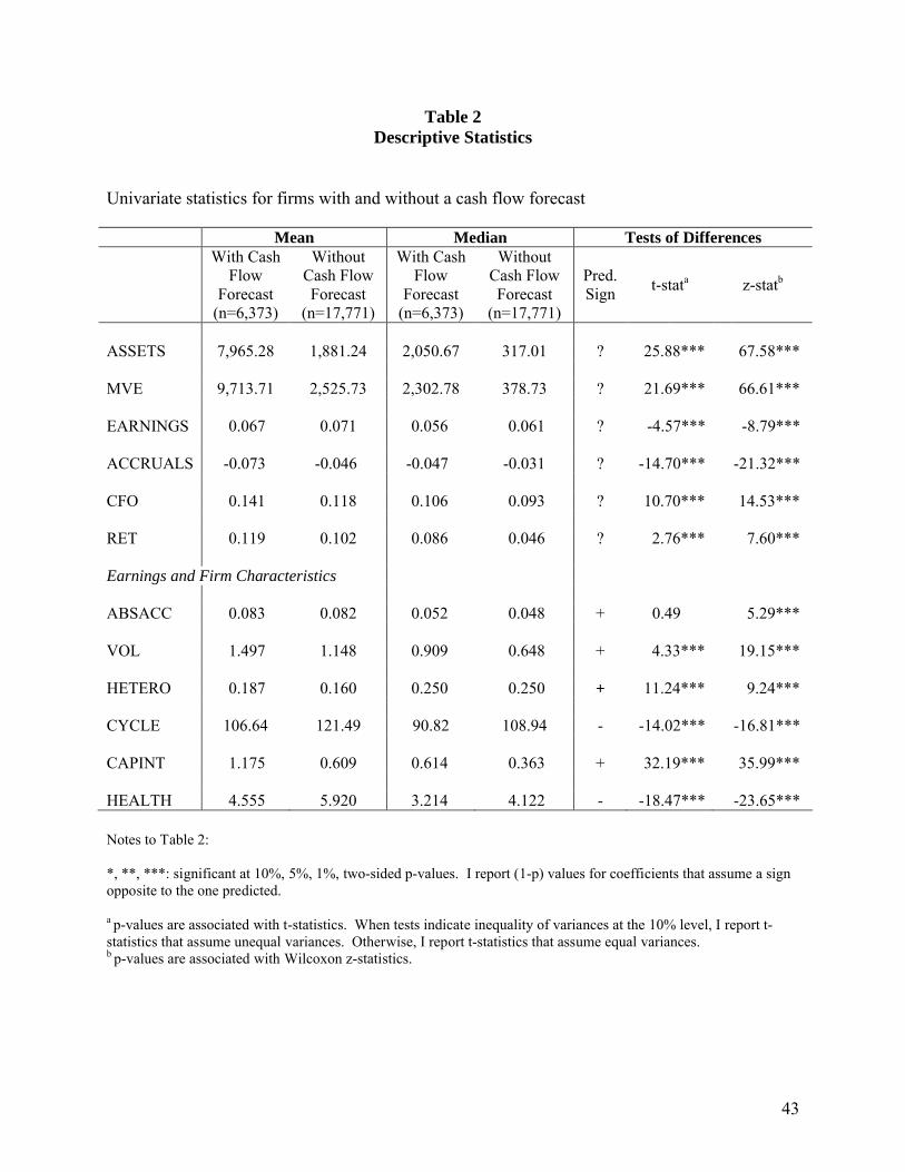
that follow. Table 2 reports the descriptive statistics for these variables, as well as other
variables of interest (total assets and market value of equity). To mitigate the effect of outliers,
all continuous variables are winsorized at the 1% and 99% levels.
Table 2 reveals that firms with a cash flow forecast are larger than firms without a cash
flow forecast, both in terms of total assets and market value. These firms also report earnings
17
that are slightly lower than firms without a cash flow forecast. Firms with cash flow forecasts
also report slightly lower (higher) accruals (operating cash flows). I investigate this difference in
more detail in Section 5.
Consistent with DeFond and Hung (2003), I find that firms with a cash flow forecast
display characteristics consistent with operating cash flows being relatively useful. These firms
exhibit accruals that are larger in absolute value, report more volatile earnings, are more likely to
use different accounting methods than their industry peers, are more capital intensive, and have
worse financial health. Furthermore, firms with a cash flow forecast have shorter trade cycles.
4. Empirical analyses
4.1 Factor analysis
The purpose of the factor analysis procedure is to (a) combine the six cross-sectional
determinants of the usefulness of cash flow information into one parsimonious variable, and (b)
extract the common portion of each of these variables. The resulting factor score presumably
incorporates the portion of each of these six variables that represents “usefulness of cash flow
information.”3
Panel A of Table 3 reports the factor loadings of the six cross-sectional variables. The
highest loadings correspond with HEALTH, CAPINT, and ABSACC (loadings of 0.700, 0,657,
and 0.633, respectively). CYCLE and HETERO also load relatively strongly with factor
loadings of 0.410 and 0.248, respectively. The only variable that does not have a strong loading
3 An alternative method of capturing CFUSE would be to regress the cash flow forecast indicator variable on all of the cross-sectional determinants of cash flow usefulness and use the predicted values that result from the model as my CFUSE measure. Such a procedure, however, would yield a variable measuring the likelihood that analysts issue a cash flow forecast for that particular firm-year, rather than a measure capturing the usefulness of the firm’s underlying cash flow data. For purposes of this study, I want a measure that captures the usefulness of the underlying cash flow information. Such a measure should be independent of analysts’ behavior and/or willingness to issue a cash flow forecast. Factor analysis is well-suited for this purpose.
18
is VOL (0.092). Overall, the factor score accounts for 26% of the variance in these six cross-
sectional variables.
Given that VOL has such a low correlation with the resulting factor score (CFUSE), I
also report the factor loadings when VOL is excluded from the analysis. When only the
remaining five variables are considered, the factor score accounts for 31% of the variance
associated with these variables. In the tests that follow, I use the original factor score (including
VOL), and refer to this score as ‘CFUSE.’4
To validate the success of the factor analysis procedure, I first replicate the results in
DeFond and Hung (2003). They find that cash flow forecasts are more common for firms with
large accruals, volatile earnings, heterogeneous accounting choices relative to industry peers,
capital-intensive firms, and firms in distress. I add trade cycle (CYCLE) to the model and run
where Fit is an indicator variable equal to 1 if analysts issued a cash flow forecast for firm i in
year t, and 0 otherwise, and all other variables are as defined in Appendix A. Table 3, Panel B
reports the results from this regression. Consistent with DeFond and Hung (2003), I find that
ACCRUALS, CYCLE, CAPINT, and HEALTH are significant determinants of a cash flow
forecast. These variables explain 18.8% of the variation in the presence of a cash flow forecast.5
When I replace the six cross-sectional determinants of a cash flow forecast with CFUSE, I find
that this model explains 18.1% of the variation in the presence of a cash flow forecast. The fact
that the explanatory power of the model is essentially the same when CFUSE is used in place of
4 All results are qualitatively unchanged when the five-variable factor score (excluding VOL) is used. 5 In DeFond and Hung (2003), they report pseudo-R2 values ranging from 12% and 25%, depending on the year.
19
the cross-sectional determinants suggests that the factor analysis procedure does a reasonable job
of summarizing and extracting the relevant portion of these variables.6
In Table 3, Panel C, I report the descriptive statistics of CFUSE across firms with
(without) a cash flow forecast. As expected, firms with a cash flow forecast have significantly
higher factor loadings (CFUSE values) than do firms without a cash flow forecast (t-stat =
28.34).
Given that DeFond and Hung (2003) find that many of the cross-sectional variables that
comprise the factor score are highly associated with the presence of a cash flow forecast, it is
reasonable to question whether F and CFUSE are truly unique variables. In Table 3, Panel D, I
examine the degree to which the presence of a cash flow forecast is associated with the factor
score. To examine this issue, each year I rank firm-year observations by CFUSE, and classify
firm-years as having a “low” (“high”) factor score if its factor score is below (above) the median
factor score for that year. Similarly, I identify firm-years that have (“yes”) or do not have (“no”)
a cash flow forecast. This results in the 2x2 table displayed in Panel D of Table 3.
Of the 6,373 firm-years with a cash flow forecast, 38% of them are classified as having a
“low” factor score. Additionally, of the firm-years classified as having a “high” factor score,
only 33% of them have a cash flow forecast. Therefore, while F and CFUSE are certainly
related, many firm-years with a cash flow forecast are not identified as having useful cash flow
information. Similarly, many firm-years without a cash flow forecast are identified as having
useful cash flow information.
These figures are consistent with the previous discussion in Section 2.3 of the small
likelihood that the variables identified by DeFond and Hung (2003) fully explain analysts’
6 The inclusion of size accounts for substantial explanatory power in Equation 1. When size is excluded, the pseudo-R2 of Equation 1 is 5.4%. When size is excluded and CFUSE is used in place of the six cross-sectional variables, the pseudo-R2 is 3.2%.
20
decisions to issue a cash flow forecast. As previously discussed, brokerage and analyst
characteristics (which are independent of the usefulness of the underlying cash flow information)
partially determine whether a firm has a cash flow forecast (Ertimur and Stubben 2006).
Specifically, analysts employed by large brokerage firms are more likely to issue cash flow
forecasts simply because these analysts have more resources available to them. Consistent with
this notion, in untabulated results I find that cash flow forecasts for firms with a low CFUSE
score are more likely to be issued by analysts employed by large brokerage firms than are cash
flow forecasts for firms with a high CFUSE score. This is consistent with firms (particularly
firms without relatively useful cash flow information) receiving cash flow forecasts for reasons
other than their accounting and economic characteristics. More generally, these results motivate
an investigation into the effect of a cash flow forecast (F) and the effect of useful cash flow
information (CFUSE) on the pricing of the accrual and cash components of earnings.
4.2 The effect of a cash flow forecast on the pricing of earnings components
My first hypothesis predicts that investors place more (less) weight on the cash (accrual)
component of earnings for firms with a cash flow forecast. I test this hypothesis in two ways.
where Fit is an indicator variable equal to 1 if analysts issued a cash flow forecast for firm i in
year t, and 0 otherwise, EARNINGSit is earnings before extraordinary items for firm i in year t,
and CFOit is operating cash flows for firm i in year t. Given that earnings is the sum of accruals
7 Prior literature documents that earnings response coefficients are a function of firm characteristics (Collins and Kothari 1989; Easton and Zmijewski 1989). I do not control for these factors because I am testing for the differential market response to the accrual and cash components of earnings. As such, there is no reason to suspect the relative accrual and cash flow response coefficients vary with these firm characteristics.
21
and operating cash flows, the coefficient on EARNINGS (β1) can be interpreted as the weight
investors place on both the accrual and cash components of earnings, and the coefficient on CFO
(β3) can be interpreted as the incremental weight placed on the cash component of earnings. As a
result, H1 predicts that β2 will be negative and that β4 will be positive, consistent with investors
placing relatively less (more) weight on the accrual (cash) component of earnings for firms with
a cash flow forecast.
I report the results from estimating Equation 2 in Panel A of Table 4. As a baseline, I
first estimate Equation 2 without the interacted terms as Model 1 in Table 4. Consistent with
prior research, the earnings response coefficient (ERC) is between 2 and 3 (2.42). The
coefficient on operating cash flows is 0.20. This implies that on average, each dollar of earnings
(accruals plus cash) is associated with a $2.42 stock price reaction, and that each dollar of cash
earnings is incrementally associated with a $0.20 stock price reaction.
I test H1 by estimating Equation 2 (Table 4, Model 2). Consistent with H1, I find that
investors place relatively less weight on the accrual component of earnings and relatively more
weight on the cash component of earnings for firms with a cash flow forecast. This finding
implies that investors behave as if cash (accrual) earnings are more (less) relevant to firm value
for firms with a cash flow forecast. In fact, the accrual component of earnings of firms without a
cash flow forecast receives approximately 75% more weight than the accrual component of
earnings of firms with a cash flow forecast. Additionally, the weight on the cash component of
earnings more than doubles for firms with a cash flow forecast. These results are consistent with
DeFond and Hung (2003, Table 5, Panel B).
However, the results from estimating Equation 2 alone are not sufficient to conclude that
the cash flow forecast itself is the cause of the increased (decreased) weight associated with the
22
cash (accrual) components of earnings. While it is possible that these results are consistent with
H1, it is also possible that investors are responding to the firms’ accounting and economic
characteristics that drove analysts to issue the cash flow forecast (rather than responding to the
cash flow forecast itself).
Accordingly, to more completely test H1, I examine whether the weights investors place
on the cash and accrual components of earnings change after the initiation of cash flow coverage.
For each firm, I identify the first year in which cash flow forecasts appear on I/B/E/S, and label
this year the “initial” year. The three years before this initial year are labeled the “pre” period,
while the initial year and the two years following the initial year are the “post” period. I require
that each firm has at least one valid observation in both the “pre” and “post” periods to be
included in the analysis. Choosing three-year windows allows investors enough time to
incorporate the presence of a cash flow forecast into their valuation judgments, while limiting the
possibility of a fundamental shift in the firm’s environment that caused analysts to begin issuing
cash flow forecasts and investors to alter the weight they assign to the earnings components. I
where CFUSEit is the factor score (representing the usefulness of cash flow information) for firm
i in year t, and all other variables are as defined previously. H2 predicts investors place more
(less) weight on the cash (accrual) component of earnings when the factor score is relatively
high. In particular, I predict that β2 (β4) will be negative (positive).
The results of testing H2 are reported in Panel A of Table 4 as Model 4. Consistent with
H2, I find that investors place relatively less weight on the accrual component of earnings for
firms with relatively useful cash flow information (β2 = -0.76). I find a slight differential in the
weighting of the cash component of earnings for firms with a high factor score (β4 = 0.03), but
this difference is only marginally statistically and economically significant.
As discussed previously, one concern is whether F and CFUSE are truly unique variables.
To provide further evidence on this issue, I run Equation 4 separately for firms with and without
a cash flow forecast. If CFUSE is nothing more than a substitute for F, I would not expect it to
successfully load among firms without a cash flow forecast. In untabulated results, I find that
8 One alternative explanation for this result is that there is an economy-wide shift in the weight investors assign to the cash and accrual components of earnings, potentially because of the Enron and WorldCom scandals. As a result, I also run Equation 2 separately for firms that received their first cash flow forecast before (after) January 1, 2002. The results from estimating the model over both sub-periods yields qualitatively similar results.
24
among firms without a cash flow forecast, CFUSE performs well in identifying firms for which
investors assign a differential weighting to the earnings components. In fact, the results across
both sub-samples (firms with a cash flow forecast and firms without a cash flow forecast) are
qualitatively similar, with the magnitude of the differential weighting actually stronger for firms
without a cash flow forecast. These results substantiate the success of CFUSE in capturing
factors affecting the usefulness of the underlying cash flow information. Additionally, this result
further suggests that F and CFUSE are indeed unique variables.
4.4 Cash flow forecasts and cash flow usefulness – Incremental and conditional analyses
Incremental analysis
The results reported in section 4.2 offer support for the notion that that the presence of a
cash flow forecast affects the weight investors assign to the cash and accrual components of
earnings (H1). Additionally, I find support in section 4.3 for the idea that the usefulness of the
underlying cash flow information is associated with increased (decreased) weight on the cash
(accrual) components of earnings (H2). The question remains, however, as to whether these two
results are incremental to each other. I examine whether the impact of a cash flow forecast on
investors’ pricing of earnings is incremental to the impact of the underlying cash flow
information, and vice versa. To empirically address this issue, I estimate the following
where CFOit is cash from operations for firm i in year t, TAit-1 is total assets for firm i in year t-1,
and Salesit is total sales revenue for firm i in year t. I estimate this model for each year and
9 See Appendix B for a more detailed description of this model.
29
industry grouping.10 For each firm-year, abnormal cash from operations (ABN_CFO) is the
difference between reported cash from operations and the predicted value of cash from
operations that results from the estimation of Equation 9. This method of estimating abnormal
operating cash flows is consistent with the methodology employed by Roychowdhury (2006).11
In Table 6, I report the mean coefficients across industry-years from estimating Equation
9. The coefficients are consistent with the predictions made by Dechow et al. (1998). The
coefficient on Salesit/TAit-1 is significantly positive, consistent with operating cash flows being
an increasing function of current sales revenue. The mean coefficient on ∆Salesit/TAit-1 is
marginally different from zero.
5.2 Abnormal operating cash flows
My purpose is to assess the degree to which firms with cash flow forecasts report
abnormally high operating cash flows. H3 predicts that because of the increased emphasis
investors and analysts place on operating cash flows, firms with a cash flow forecast will report
abnormally high operating cash flows.
To test this hypothesis, I first evaluate the mean level of ABN_CFO for firms with a cash
flow forecast relative to firms without a cash flow forecast. Table 7, Panel A reveals that firms
with a cash flow forecast report mean (median) abnormal operating cash flows of 5.4% (4.1%) of
total assets. Given that the mean (median) level of operating cash flows for firms with a cash
flow forecast is 10.4% (10.2%) of total assets (untabulated), this is an economically large level of
abnormal cash flows. Firms without a cash flow forecast, on the other hand, report mean
(median) abnormal operating cash flows of -1.4% (1.8%) of total assets. The difference between
10 I use the two-digit SIC code to identify industries. A minimum of 10 observations in each industry-year grouping is required. 11 Note that because this model is estimated separately for each industry, it controls for any determinants of normal operating cash flows that are clustered by industry.
30
both the mean and median levels of ABN_CFO between firms with and without a cash flow
forecast is both statistically and economically significant. This result provides initial support for
my hypothesis that firms with cash flow forecasts report artificially high operating cash flows.
One alternative explanation for the difference in ABN_CFO reported in Panel A of Table
7 is that analysts are able to identify firms with abnormally large operating cash flows and
choose to issue cash flow forecasts for these firms. In such a scenario, abnormal levels of
operating cash flows would not be consistent with managers boosting operating cash flows
because of the cash flow forecast, but rather would imply that firms have a cash flow forecast
because of their abnormally high cash from operations.
To investigate this possibility, I perform two tests. First, I compare the abnormal
operating cash flows for the three years before the initial cash flow forecast to the abnormal
operating cash flows for the year of the initial cash flow forecast and the following two years.12 I
find that after the initiation of cash flow forecasts, firms report significantly higher abnormal
operating cash flows (untabulated). On average, abnormal cash flows are 1.2% of total assets
higher after analysts issue the first cash flow forecast.
Second, I isolate all firms with a cash flow forecast, and examine whether the level of
abnormal cash flows varies as a function of the degree to which firms meet or beat analysts’
earnings expectations.13 If managers of firms with a cash flow forecast are managing cash flows
for opportunistic reasons, I would expect to find firms that meet or barely beat analysts’ earnings
forecasts to have higher abnormal cash flows than firms in other regions of the meet/beat
distribution.
12 I again impose the constraint that to be included in this analysis, a firm must have at least one valid observation before a cash flow forecast was issued and at least one valid observation in the three years beginning with the first year a cash flow forecast was issued.13 As a proxy for analysts’ earnings expectations, I use the last earnings forecast issued prior to the firm’s earnings announcement.
31
I divide all firms with a cash flow forecast into four groups, based on the difference
between reported EPS and analysts’ expectation of EPS. MISS corresponds to all firm-years
with reported EPS below forecasted EPS. SMALL corresponds to all firm-years with forecast
errors between $0.00 and $0.02, inclusive. MEDIUM corresponds to all firm-years with forecast
errors between $0.02 and $0.04, and LARGE corresponds to all firm-years with forecast errors
larger than $0.04. Panel B of Table 7 reveals that the mean (median) values of abnormal
operating cash flows vary as one would expect if managers are managing operating cash flows
flow values are highest for firms in the SMALL group (7.3% of total assets), with lower values
of ABN_CFO as the earnings forecast error diverges from zero.
I find that the mean (median) values of abnormal operating cash flows are significantly
different across all groups, as expected, with one exception. The mean abnormal operating cash
flow for firms in the SMALL group is not significantly higher than it is for firms in the
MEDIUM group. The median values across these two groups, are, however, statistically
different (p=0.033). Additionally, I find abnormal cash flow values for the SMALL group are
significantly higher than the abnormal cash flow values for a group comprised of both MEDIUM
and LARGE firms. This finding supports the notion that firms with a cash flow forecast report
artificially high to meet or beat analysts’ earnings forecasts. In addition, given that the abnormal
cash flow values of firms in the SMALL group are higher than those of firms in either the
MEDIUM or LARGE groups, this result does not appear to be driven by performance.
Interestingly, this pattern of abnormal operating cash flows around the earnings forecast
error is not apparent when evaluated relative to the cash flow forecast error. Firms that beat the
cash flow forecast by a wide margin report higher abnormal cash flows than do firms that meet
32
or barely beat the cash flow forecast (untabulated). This result suggests that the cash flow
forecast is not a key target even for firms with a cash flow forecast and that analysts’ earnings
forecasts remain the primary benchmark. This finding is consistent with recent survey evidence
suggesting that executives rank earnings as the most important performance metric reported to
outsiders (Graham et al. 2005).
Lastly, I investigate whether the propensity to meet/beat analysts’ forecasts with
abnormally high operating cash flows is greater for firms with a cash flow forecast. To do this, I
isolate all firms (with and without a cash flow forecast) in the SMALL group, and compare
ABN_CFO values between firms with and without a cash flow forecast. These results are
reported in Panel C of Table 7. I find that while firms in the SMALL group that do not have a
cash flow forecast also appear to employ abnormal operating cash flows to meet analysts’
earnings forecasts (mean = 0.053), firms in the SMALL group that have a cash flow forecast
report relatively higher abnormal operating cash flows (mean = 0.073). This result supports H3
and suggests that firms with a cash flow forecast are more likely to opportunistically boost
abnormal cash flows to meat/beat analysts’ earnings forecasts.
This finding complements the findings of McInnis and Collins (2006). They report that
firms with a cash flow forecast are less likely to use discretionary accruals to meet/beat analysts’
earnings expectations. They argue that because both an earnings forecast and a cash flow
forecast result in an implicit accrual forecast, firms with a cash flow forecast have more
transparent accruals and will be less likely to manage accruals. They find results supporting their
prediction. Consistent with their finding, I find that firms with a cash flow forecast are more
likely to use abnormal cash flows to meet earnings targets. The results of this paper suggest,
33
however, that capital market pressures (a higher (lower) weight on the cash (accrual) component
of earnings) are a potential source of this behavior.
6. Conclusion
I examine the effect of cash flow forecasts on investors’ pricing and managers’ reporting
of the cash and accrual components of earnings. Analysts’ cash flow forecasts are becoming an
increasingly common fixture in the current information environment. This paper adds to our
understanding of the impact of these forecasts on both investors’ pricing behavior and managers’
reporting decisions.
I find that the cash (accrual) component of earnings is more (less) associated with
contemporaneous stock returns for firms with a cash flow forecast, and that this relation is even
stronger for firms with relatively useful cash flow information. Additionally, I find that investors
place relatively less weight on the accrual component of earnings immediately following
analysts’ initial cash flow forecast. Overall, the mere presence of a cash flow forecast affects
investors’ pricing of earnings, and this effect is incremental to the effect of the usefulness of the
underlying cash flow information. These findings add to the literature on the role of analysts in
investors’ use of accounting information, and imply that even analysts’ decisions to issue cash
flow forecasts have valuation implications.
Furthermore, for firms with a cash flow forecast, the cash (accrual) components of
earnings is more (less) predictive of future firm prospects. This implies that (a) when valuing
firms with a cash flow forecast, investors are justified in assigning more (less) weight to the cash
(accrual) components of earnings, and (b) analysts successfully identify firms with more
predictive cash flow information and issue cash flow forecasts for these firms. Firms deemed to
34
have useful cash flow information also report cash flows information that is more predictive of
future cash flows.
Lastly, I find that managers of firms with a cash flow forecast are more likely to
artificially boost reported cash flows than are managers of firms without a cash flow forecast.
While a considerable body of research has analyzed earnings management through the
manipulation of accruals, I document a setting where the management of operating cash flows is
likely to be a concern. In doing so, I further highlight the impact of capital market pressures on
managers’ propensity to artificially boost earnings. These results suggest that the nature of the
capital market pressure can impact the mechanism through which earnings are managed.
This paper has important implications for the role of analysts in the capital markets. I
document that while investors alter their assessments of accounting information based upon
analysts’ decisions to issue a cash flow forecast, managers also react by artificially boosting
reported operating cash flows. Future studies can focus on other performance metrics (e.g., sales
revenue) and the valuation and reporting implications of analysts’ revenue forecasts. Such an
inquiry would indicate whether the results reported in this paper are unique to cash flow
information or whether these findings are generalizable to all accounting metrics forecasted by
analysts. Additionally, future work can investigate the contracting (e.g., compensation)
implications of having a cash flow forecast, and whether contracts reflect an increased focus on
performance measures that are forecast by analysts.
35
References
Altman, E. 1968. Financial rations, discriminant analysis, and the prediction of corporate bankruptcy. The Journal of Finance 23: 589-609.
Barth, M., W. Beaver, and W. Landsman. 1998. Relative valuation roles of equity book value and net income as a function of financial health. Journal of Accounting and Economics25: 1-34.
Barth, M., D. Cram, and K. Nelson. 2001. Accruals and the prediction of future cash flows. The Accounting Review 76: 27-58.
Bartov, E., D. Givoly, and C. Hayn. 2002. The rewards to meeting or beating earnings expectations. Journal of Accounting and Economics 33: 173-204.
Beaver, W. 1966. Financial ratios as predictor of failure. Journal of Accounting Research 4: 71-111.
Biddle, G., C. Seow, and A. Siegel. 1995. Relative versus Incremental Information Content. Contemporary Accounting Research 12: 1-23.
Bowen, R., D. Burgstahler, and L. Daley. 1987. The incremental information content of accrual versus cash flows. The Accounting Review 61: 723-747.
Burgstahler, D., and I. Dichev. 1997. Earnings, adaptation, and book value. The Accounting Review 72: 187-215.
Chaney, P., and C. Lewis. 1995. Income smoothing and underperformance in initial public offerings. Journal of Corporate Finance 4: 1-29.
Christie, A., and J. Zimmerman. 1994. Efficient and opportunistic choices of accounting procedures: Corporate control contests. The Accounting Review 69: 539-566.
Clement, M. 1999. Analyst forecast accuracy: Do ability, resources, and portfolio complexity matter? Journal of Accounting and Economics 27, 285-303.
Collins, D., and S. Kothari. 1989. An analysis of the intertemporal and cross-sectional determinants of the earnings response coefficients. Journal of Accounting and Economics 11:143-181.
Dechow, P. 1994. Accounting earnings and cash flows as measures of firm performance: The role of accounting accruals. Journal of Accounting and Economics 18: 3-42.
Dechow, P., and I. Dichev. 2002. The quality of accruals and earnings: The role of accrual estimation errors. The Accounting Review 77: 35-59.
36
Dechow, P., S. Kothari, and R. Watts. 1998. The relation between earnings and cash flows. Journal of Accounting and Economics 25: 133-168.
DeFond, M., and M. Hung. 2003. An empirical analysis of analysts’ cash flow forecasts. Journal of Accounting and Economics 35: 73-100.
DeFond, M., and J. Jiambalvo. 1994. Debt covenant violation and manipulation of accruals: accounting choice in troubled companies. Journal of Accounting and Economics 17: 145-176.
Dhaliwal, D., C. Gleason, and L. Mills. 2004. Last chance earnings management: Using the tax expense to achieve earnings targets. Contemporary Accounting Research 24: 433-459.
Easton, P., and M. Zmijewski. 1989. Cross-sectional variation in the stock market response to the announcement of accounting earnings. Journal of Accounting and Economics 11: 117-141.
Ertimur, Y., and S. Stubben. 2006. Analysts’ incentives to issue revenue and cash flow forecasts. Working paper, Duke University and University of North Carolina, Chapel Hill.
Graham, J., C. Harvey, and S. Rajgopal. 2005. The economic implications of corporate financial reporting. Journal of Accounting and Economics 40: 3-73.
Hayn, C. 1995. The information content of losses. Journal of Accounting and Economics 20: 125-153.
Healy, P. 1985. The effect of bonus schemes on accounting decisions. Journal of Accounting and Economics 7: 85-107.
Matsunaga, S., and C. Park. 2001. The effect of missing a quarterly earnings benchmark on the CEO’s annual bonus. The Accounting Review 76: 313-332.
McInnis, J., and D. Collins. 2006. Do cash flow forecasts deter earnings management? Working paper, University of Iowa.
McVay, S. 2006. Earnings management using classification shifting: an examination of core earnings and special items. The Accounting Review 81: 501-531.
Ohlson, J. 1980. Financial ratios and the probabilistic prediction of bankruptcy. Journal of Accounting Research 18: 109-131.
Ohlson, J. 1995. Earnings, book values, and dividends in equity valuation. Contemporary Accounting Research 11: 661-687.
37
Roychowdhury, S. 2006. Earnings management through real activities manipulation. Journal of Accounting and Economics 42: 335-370.
Securities and Exchange Commission v. Dynegy Inc. 2002. Civil Action No. H-02-3623, U.S.D.C./Southern District of Texas (Houston Division).
Skinner, D., and R. Sloan. 2002. Earnings surprises, growth expectations, and stock returns or don’t let and earnings torpedo sink your portfolio. Review of Accounting Studies 7: 289-312.
Standard & Poor’s. 2002. Corporate ratings criteria.
Teoh, S., I. Welch, and T. Wong. 1998. Earnings management and the long-run underperformance of seasoned equity offerings. Journal of Financial Economics 50: 63-100.
Tucker, J., and P. Zarowin. 2006. Does income smoothing improve earnings informativeness? The Accounting Review 81: 251-270.
38
Appendix AVariable Definitions
ABSACC: |Income before extraordinary items minus cash from operations|, scaled by total assets. This variable is calculated as of year t.
VOL: The coefficient of variation of earnings measured over year t and the previous 4 years scaled by the coefficient of variation of operating cash flows measured over the same period. This variable is calculated as (|standard deviation of earnings / mean of earnings|) / (|standard deviation of operating cash flows / mean of operating cash flows|).
HETERO: An index ranging from 0 to 1 that captures the similarity of a firm’s accounting choices in year t relative to other firms in the same industry. In each year, I examine five accounting choices, and for each accounting choice, assign the firm a value of one if its chosen method differs from the most frequently chosen method in its industry group, and zero otherwise. The five accounting choices are: (1) inventory valuation, (2) investment tax credit, (3) depreciation, (4) successful-efforts vs. full-cost for companies with extraction activities, and (5) purchase vs. pooling. The five scores are summed and divided by the number of accounting choices in the industry (which for some industries is less than five). Higher (lower) index values are consistent with heterogeneous (homogeneous) accounting choices. This calculation is consistent with DeFond and Hung (2003).
CYCLE: The trade cycle of the firm, calculated as (Dechow 1994):
where AR is accounts receivable (Compustat annual #2), INV is inventory (Compustat annual #3), AP is accounts payable (Compustat annual #70), Sales is total sales revenue (Compustat annual #12), COGS is cost of goods sold (Compustat annual #41), and Purchases is calculated as INVt – INVt-1 + COGS. In the empirical tests that follow, I multiply the CYCLE by negative one, such that higher values are consistent with cash flow information being a more useful performance metric. This variable is calculated as of year t.
CAPINT: The ratio of gross property, plant, and equipment (Compustat annual #7) divided by sales revenue (Compustat annual #12). This variable is calculated as of year t.
39
Appendix A (cont.)Variable Definitions
HEALTH: I estimate Altman’s Z-score in year t as a proxy for financial health. Consistent with Altman (1968), the Z score equals 1.2*(Net working capital / Total assets) + 1.4*(Retained earnings / Total assets) + 3.3*(Earnings before interest and taxes / Total assets) + 0.6*(Market value of equity / Book value of liabilities) + 1.0*(Sales / Total assets). Lower Altman’s Z-scores indicate poorer financial health. In the empirical tests that follow, I multiply the Altman’s Z-scores by negative one, such that higher values are consistent with cash flow information being a more useful performance metric.
F: An indicator variable equal to 1 if the firm has a cash flow forecast in year t, and 0 otherwise.
CFUSE: The factor score in year t from a factor analysis performed on the following six variables: ACCRUALS, VOL, HETERO, CYCLE, CAPINT, and HEALTH.
CFO: Cash from operations (Compustat annual #308) in year t, scaled by beginning-of-period price (Compustat #199).
EARNINGS: Income before extraordinary items (Compustat annual #18) in year t, scaled by beginning-of-period-price (Compustat #199).
RET: 12-month CRSP buy-and-hold stock returns for beginning 3 months after fiscal-year end.
40
Appendix BModeling “normal” operating cash flows
I use the model outlined in Dechow et al. (1998) to derive estimates of normal cash from operations for each firm-year. In their model, they relate a firm’s operating cash flows to its earnings and accruals. In doing so, they make the following simplifying assumptions about the accounting process: (i) sales follow a random walk, (ii) there are no fixed costs, (iii) the proportion of sales that remains uncollected at the end of the period is constant, (iv) target inventories is a constant proportion of next period’s sales, and (v) a constant proportion of the firm’s purchases remain unpaid at the end of the period.
They begin by expressing earnings as a percentage of total sales.
Et = πSt,
where π is the net profit margin. Consequently, total expenses vary with sales and are (1- π)St.
Accounts receivable is as constant fraction, α, of current sales.
ARt = αSt.
Inventory consists of a target level and a deviation from that target. Target inventory is a constant fraction, γ1, of next period’s cost of sales. Since sales are assumed to follow a random walk, target inventory is γ1(1-π)St, where γ1>0. If the firm is able to successfully change inventory levels in response to changes in sales, inventory will increase by γ1(1-π)∆St, where ∆St = St – St-1 = εt. However, as actual sales in period t differ from expected sales levels, inventory will not always be at the target level. This deviation from target inventory can be expressed as γ2γ1(1-π)(εt), where γ2 is a constant that captures the speed with which a firm adjusts its inventory to its target level. As a result, actual inventory levels at the end of the period are expressed as follows:
INVt = γ1(1 – π)St - γ2γ1(1 – π)εt.
Accounts payable are a constant fraction, β, of the period’s purchases, where purchases are (cost of goods sold + ending inventory – beginning inventory). Purchases can be expressed as:
Pt = (1 – π)St + γ1(1 – π)εt - γ2γ1(1 – π)∆εt.
The first term represents the purchases necessary for the current period sales. The second term consists of the purchases necessary to adjust inventory for the change in target inventory due to changes in sales, and the third term represents the deviation from target inventory. As a result, accounts payable is
Dechow et al. (1998) simplify this expression by noting that the second and third terms are close to zero and likely to be negligible in practice. The remaining term represents the firm’s accruals and is the firm’s operating cash cycle, [α + (1 – π)γ1 – β(1 – π)], multiplied by the sales shock for the period, εt. If the operating cash cycle is denoted by δ, earnings can be expressed as
Et = CFOt + δεt.
It then follows that cash from operating is
CFOt = Et – At = πSt – δεt = πSt – δ(St – St-1).
This equation expresses operating cash flows as a function of current period sales (St) and the change in sales from the prior period (St – St-1). This is the equation I use to estimate “normal” cash from operations.
42
Table 1Sample Description
Panel A: Number (%) of firms with a cash flow forecast – all firms
HEALTH 4.555 5.920 3.214 4.122 - -18.47*** -23.65***
Notes to Table 2:
*, **, ***: significant at 10%, 5%, 1%, two-sided p-values. I report (1-p) values for coefficients that assume a sign opposite to the one predicted.
a p-values are associated with t-statistics. When tests indicate inequality of variances at the 10% level, I report t-statistics that assume unequal variances. Otherwise, I report t-statistics that assume equal variances. b p-values are associated with Wilcoxon z-statistics.
44
Table 2 (cont.)Descriptive Statistics
Notes to Table 2 (cont.):
Definition of variables:ASSETS = total assets (Compustat #6) in year t.MVE = market capitalization in year t, defined as stock price times the number of shares outstanding
(Compustat #199 * Compustat #25). EARNINGS = net income before extraordinary items (Compustat #18) in year t, scaled by beginning-of-period
price (Compustat #199).ACCRUALS = total accruals in year t, calculated as net income before extraordinary items (Compustat #18)
minus cash from operations (Compustat #308), scaled by beginning-of-period price (Compustat #199).
CFO = cash from operations (Compustat #308) in year t, scaled by beginning-of-period price (Compustat #199).
RET = the twelve-month buy-and-hold stock return beginning three months after fiscal year end. ABSACC = the absolute value of total accruals in year t, measured as |income before extra-ordinary items
minus cash from operations|, scaled by total assets.VOL = the volatility of earnings in year t, measured as (|standard deviation of earnings / mean of
earnings|) / (|standard deviation of operating cash flows / mean of operating cash flows|), measured over year t and the previous 4 years.
HETERO = an index ranging from 0 to 1 that captures the similarity of a firm’s accounting choices in year trelative to other firms in the same industry. For each of the following five accounting choices, I assign the firm a value of one if its chosen method differs from the most frequently chosen method in its industry group, and zero otherwise. The five accounting choices are: (1) inventory valuation, (2) investment tax credit, (3) depreciation, (4) successful-efforts vs. full-cost for companies with extraction activities, and (5) purchase vs. pooling. The five scores are summed and divided by the number of accounting choices in the industry (which for some industries is less than five). Higher (lower) index values are consistent with heterogeneous (homogeneous) accounting choices.
CYCLE = trade cycle of the firm, calculated as (Dechow 1994):(ARt + ARt-1)/2 + (INVt + INVt-1)/2 – (APt + APt-1)/2
Sales/360 COGS/360 Purchases/360where AR is accounts receivable (Compustat annual #2), INV is inventory (Compustat annual #3),AP is accounts payable (Compustat annual #70), Sales is total sales revenue (Compustat annual #12), COGS is cost of goods sold (Compustat annual #41), and Purchases is calculated as INVt –INVt-1 + COGS.
CAPINT = the ratio of gross property, plant, and equipment (Compustat #7) divided by sales revenue (Compustat #12) in year t.
HEALTH = Altman’s Z-score as a proxy for financial health. Consistent with Altman (1968), the Z-score in year t equals 1.2*(Net working capital / Total assets) + 1.4*(Retained earnings / Total assets) + 3.3*(Earnings before interest and taxes / Total assets) + 0.6*(Market value of equity / Book value of liabilities) + 1.0*(Sales / Total assets). Lower Altman’s Z-scores indicate poorer financial health.
45
Table 3Factor Analysis for Determinants of the Usefulness of Operating Cash Flow Information
Panel A: Factor loadings using principal components analysis
Panel C: Univariate statistics for the factor score (CFUSE)
Mean Median Std. Dev. t-stata z-statb
With Cash Flow Forecast
0.320 0.160 1.086
Without Cash Flow Forecast
-0.115 -0.171 0.94128.34*** 28.56***
46
Table 3 (cont.)Factor Analysis for Determinants of Usefulness of Operating Cash Flow Information
Panel D: Relation between cash flow forecast and factor score (CFUSE)
Cash Flow ForecastNo Yes TOTAL
Low 9,649 2,420 12,069Factor Score (CFUSE) High 8,122 3,953 12,075
TOTAL 17,771 6,373 24,144
Notes to Table 3:
*, **, ***: significant at 10%, 5%, 1%, two-sided p-values. I report (1-p) values for coefficients that assume a sign opposite to the one predicted.
a p-value is associated with the t-statistic. b p-value is associated with Wilcoxon z-statistics.
Definition of Variables: MVE = market capitalization in year t, defined as stock price times the number of shares outstanding
(Compustat annual #199 * Compustat annual #25). ABSACC = the absolute value of total accruals in year t, measured as |income before extra-ordinary items
minus cash from operations|, scaled by total assets.VOL = the volatility of earnings in year t, measured as (|standard deviation of earnings / mean of
earnings|) / (|standard deviation of operating cash flows / mean of operating cash flows|), measured over year t and the previous 4 years.
HETERO = an index ranging from 0 to 1 that captures the similarity of a firm’s accounting choices in year trelative to other firms in the same industry. For each of the following five accounting choices, I assign the firm a value of one if its chosen method differs from the most frequently chosen method in its industry group, and zero otherwise. The five accounting choices are: (1) inventory valuation, (2) investment tax credit, (3) depreciation, (4) successful-efforts vs. full-cost for companies with extraction activities, and (5) purchase vs. pooling. The five scores are summed and divided by the number of accounting choices in the industry (which for some industries is less than five). Higher (lower) index values are consistent with heterogeneous (homogeneous) accounting choices.
CYCLE = trade cycle of the firm, calculated as (Dechow 1994):(ARt + ARt-1)/2 + (INVt + INVt-1)/2 – (APt + APt-1)/2
Sales/360 COGS/360 Purchases/360where AR is accounts receivable (Compustat annual #2), INV is inventory (Compustat annual #3), AP is accounts payable (Compustat annual #70), Sales is total sales revenue (Compustat annual #12), COGS is cost of goods sold (Compustat annual #41), and Purchases is calculated as INVt –INVt-1 + COGS.
CAPINT = the ratio of gross property, plant, and equipment (Compustat #7) divided by sales revenue (Compustat #12) in year t.
HEALTH = Altman’s Z-score as a proxy for financial health. Consistent with Altman (1968), the Z-score in year t equals 1.2*(Net working capital / Total assets) + 1.4*(Retained earnings / Total assets) + 3.3*(Earnings before interest and taxes / Total assets) + 0.6*(Market value of equity / Book value of liabilities) + 1.0*(Sales / Total assets). Lower Altman’s Z-scores indicate poorer financial health.
47
Table 4Multivariate Regressions
Panel A: The effect of a cash flow forecast and CFUSE on the pricing of the earnings components – Primary analyses
Coefficients (top) and t-statistics (bottom) are reported. *, **, ***: significant at 10%, 5%, 1%, two-sided p-values. I report (1-p) values for coefficients that assume a sign opposite to the one predicted
Definition of Variables:RET = the twelve-month buy-and-hold stock return for firm i beginning three months after fiscal year
end. EARNINGS = net income before extraordinary items (Compustat #18) for firm i in year t, scaled by beginning-
of-period price (Compustat #199).CFO = cash from operations (Compustat #308) for firm i in year t, scaled by beginning-of-period price
(Compustat #199).F = an indicator variable equal to 1 if an analyst has issued a forecast of operating cash flows for
firm i in year t, and 0 otherwise.POST = an indicator variable equal to 1 for the first year and the two years following analysts’ initial
cash flow forecast for the firm, and 0 otherwise.CFUSE = a measure of the informativeness of operating cash flow information, measured as the factor
score for firm i in year t, where the factor score is based on the following variables: ABSACC, VOL, HETERO, CYCLE, CAPINT, and HEALTH.
50
Table 5The Predictive Ability of Accrual and Cash Components of Earnings
Table 5 (cont.)The Predictive Ability of Accrual and Cash Components of Earnings
Notes to Table 5:
Coefficients (top) and t-statistics (bottom) are reported. *, **, ***: significant at 10%, 5%, 1%, two-sided p-values.
Definition of Variables:RET = the twelve-month buy-and-hold stock return for firm i beginning three months after fiscal year end. EARNINGS = net income before extraordinary items (Compustat #18) for firm i in year t, scaled by beginning-of-period price (Compustat #199).CFO = cash from operations (Compustat #308) for firm i in year t, scaled by beginning-of-period price (Compustat #199).F = an indicator equal to 1 if an analyst has issued a forecast of operating cash flows for firm i in year t, and 0 otherwise.D_CFUSE = a dummy variable equal to one if firm i's CFUSE (cash flow usefulness) score is in the highest quintile in year t, and 0 otherwise.
Coefficients (top) and t-statistics (bottom) are reported. *, **, ***: significant at 10%, 5%, 1%, two-sided p-values.
Equation 9 is estimated for every industry (2-digit SIC code) every year. There are 894 separate industry-years from 1993-2005. I report the mean (median) coefficients across all industry-years. I use the standard error of the mean (median) to calculate t-statistics. I also report the mean (median) adjusted-R2 across all industry-years.
Definition of Variables:CFO = cash from operations (Compustat #308) for firm i in year t, scaled by beginning-of-period price
(Compustat #199).TA = total assets for firm i in year t-1.SALES = total sales revenue (Compustat annual #12) for firm i in year t.∆SALES = the change in total sales revenue from year t-1 to year t for firm i.
53
Table 7Abnormal Operating Cash Flows
Panel A: Abnormal operating cash flows – firms with (without) a cash flow forecast
Group N Mean Median Std. Dev. t-stata z-statb
With Cash Flow
Forecast9,874 0.054 0.041 0.182
Without Cash Flow Forecast
73,020 -0.014 0.018 0.335
30.71*** 21.28***
Panel B: Abnormal operating cash flows across the meet/beat distribution– firms with a cash flow forecast
Group Nc Mean Median Std. Dev.MISS 3,446 0.036 0.027 0.189SMALL 2,940 0.073 0.061 0.176MEDIUM 1,018 0.066 0.049 0.194LARGE 2,280 0.053 0.037 0.166
Comparison t-stata z-statb
MISS vs. SMALL 8.06*** 12.46***SMALL vs. MEDIUM -0.98 -1.84**MEDIUM vs. LARGE -1.79** -3.46***SMALL vs. (MEDIUM + LARGE) -3.46*** -6.30***
Panel C: Abnormal operating cash flows – firms with (without) a cash flow forecast – SMALL only
Group N Mean Median Std. Dev. t-stata z-statb
With Cash Flow
Forecast2,940 0.073 0.061 0.176
Without Cash Flow Forecast
10,109 0.053 0.058 0.265
4.61*** 2.01**
54
Table 7 (cont.)Abnormal Operating Cash Flows
Notes to Table 7:
*, **, ***: significant at 10%, 5%, 1%, two-sided p-values. I report (1-p) values for coefficients that assume a sign opposite to the one predicted.
a p-value is associated with the t-statistic. b p-value is associated with Wilcoxon z-statistics.c The number of observations in Panel B is slightly less than the number of observations in Panel A because for some firms, there is not enough data to calculate the earnings forecast error.
Definition of Variables:ABN_CFO = abnormal operating cash flows for firm i in year t, calculated as the difference between reported
operating cash flows (Compustat #308) and an estimate of normal operating cash flows. Normal operating cash flows are estimated as the predicted value of operating cash flows that results from estimating the following regression: CFOit/TAit-1= α0 + α1(1/TAit-1) + β1(Salesit/TAit-1) + β2(∆Salesit/TAit-1) + εit. This regression is estimated for each industry-year group from 1993-2005 that has a minimum of 10 observations.
MISS = firm-years that reported earnings below analysts’ forecast of earnings.SMALL = firm-years with an earnings forecast error between $0.00 and $0.02, inclusive.MEDIUM = firm-years with an earnings forecast error larger than $0.02 and no larger than $0.04.LARGE = firm-years with an earnings forecast error larger than $0.04.