- 27 -

http://www.ivypub.org/RSS/

Remote Sensing Science November 2013, Volume 1, Issue 3, PP.27-40

The Improved Calibration Method and Retrieval

Models Using Advanced Ground-based

Multi-frequency Microwave Sounder Jieying He†, Shengwei Zhang

Key Laboratory of Microwave Remote Sensing, Center for Space Science and Applied Research, Chinese Academy of Sciences,

Beijing 100190, China

†Email: peggy.hejieying@163.com

Abstract

The paper presents an improved ground-based atmospheric microwave sounder with multi-frequency channels. Compared to

international used atmospheric microwave sounder, the merits of the instrument is described. To derive more accurate brightness

temperature from microwave sounder observation, the paper presents 4 calibration processes in different process to perfect the

calibration, including LN2 calibration, tipping curve calibration, nonlinear correction and quasi real time calibration. Since the

close relationship between cloud and integrated water vapor and liquid water content, the paper describes several cloud-judgment

models, and presents an improved cloud modal considering all the characteristics of all cloud models. Furthermore, the objective

of this study is to test ANN (Artificial Neural Network) methodology for the problems of integrated water vapor and liquid water

path derivation, using the improved ground-based atmospheric microwave sounder brightness temperatures and surface

information such as temperature, humidity, pressure and so on. Compared to the commonly used method linear regression, this

paper built a better retrieval model using ANN theory which can be high nonlinear and provide a tool to fit function to data. The

present model gave an average RMS（Root Mean Square）error of integrated water vapor and liquid water content are less than

0.05cm and 0.5mm dependent on the actual atmospheric situation.

Keywords: Calibration; Artificial Neural Network; Integrated Water Vapor; Liquid Water Path; Root Mean Square

1 INTRODUCTION

Atmospheric integrated water vapor and liquid water content are important meteorological parameters. Water vapor

varies significantly from time to time and from space to space. The vertically integrated water vapor as well as

integrated cloud liquid water plays a key role in the study of global atmospheric circulation and evolution of clouds,

also helps one to understand the global hydrologic cycle and the earth‟s radiative balance. The amount of water

vapor in the air varies considerably, from practically none at all up to about 4 percent by volume which includes

water vapor, ozone, nitrogen, carbon dioxide argon and others. Certainly the fact is that water vapor is the source of

all clouds and precipitation which would be enough to explain its importance.

There are two traditional sounding instruments to retrieve them: radiosonde (radar) working on the ground and

remote sensing satellite working on the high spatial orbit. The former one is bulky and costly which is perplexing to

install and operate and having lower spatial and temporal resolution. The latter one has higher spatial resolution and

wider coverage. However, due to the shelter and strong absorption of cloud, as well as atmospheric opacity for

electromagnetic wave in the millimeter-wave band, satellite instrument with limitation of remote sensing technology

has a lower vertical resolution at the bottom of troposphere.

By far, ground-based atmospheric microwave sounder has been considered the best accurate and lowest-cost

instrument to retrieve integrated water vapor and liquid water content. It can be operated in a long-term unattended

- 28 -

http://www.ivypub.org/RSS/

mode under almost all weather conditions with reliable results and has a low maintenance cost. Also it has a high

resolution at the bottom of lower troposphere. With the long-term development of theory and laboratory

measurements, it has been widely used in meteorological observations and forecasting, communications, geodesy

and long-baseline interferometry, satellite validation, climate and fundamental molecular physics.

The paper mainly introduces a prototype of ground-based atmospheric microwave sounder which operates in K-band

from 22 GHz to 31 GHz and V-band from 51 GHz to 59 GHz, respectively [1]. Different from the MP3000A [2] and

RPG [3], the sounder adopts independent dual-band reflectors instead of sharing a dual-band reflector. The direct detect

type receiver is applied which is of smaller size, higher sensitivity, efficient data observing and lower nonlinear error

than the widely used superheterodyne receiver. The observing brightness temperatures from this prototype agree well

with simulated brightness temperatures according to the ground-based radiative transfer theory [4].

2 DESCRIPTION OF GROUND-BASED MULTI-CHANNEL ATMOSPHERIC MICROWAVE

SOUNDER

2.1 The design of atmospheric microwave sounder

In this paper, we mainly introduce a prototype of advanced ground based atmospheric sounder with improvements.

In this prototype, different from international commonly used microwave radiometers, the receiver system adopts

direct detect type rather than superheterodyne type which is used in almost all the microwave radiometers recently.

For the reflector-configuration, it adopts two independent reflectors in each band rather than sharing one reflector in

dual band. The description in detail has been shown in reference [1].

Microwave radiometer receiver with direct detect type mainly consists of directional coupler, RF amplifier, power

divider, band-pass filter, square law detector, integrator and video frequency amplifier. The signal accepted by

antenna is amplified and distributed into several RF channels without mixers. It uses band-pass filter to decide the

frequency for each channel. Here the bandwidths in different channels can be different. In the system, the number of

sounding-channel depends on power divider network. Different from superheterodyne type, it‟s easy to control and

operate without mixer and frequency synthesizer. The most importance, it can detect all the channels simultaneously,

therefore it has long integrated time and high scanning efficiency. Adopting independent reflectors, we design and

optimize them independently and also make the width of antenna as small as possible. With a smaller height value

and a similar width value, the whole size and whole device expense can be decreased feasible. In this configuration

mode, we can easily release the low sidelode and design the antenna in dual-band independently without frequency

segregation. The prototype has high calibration accuracy because it use independent blackbody in each band and

need not consider the dual band requirements. Furthermore, it decreases the wave loss through radome and has high

expansibility to release multi-polarization measurements.

TABLE 1 THE SPECIFICATIONS OF THE PROTOTYPE

(Ground-based multi-frequency atmospheric microwave sounder)

specification Prototype of design

Calibration resolution 1.5k

Long-term stability <1.0k/year

BT resolution 0.1-1k

BT coverage 0-400 K

Antenna resolution and side lobe

22-30 GHz

51-59 GHz

4.9 - 6.3° -24 dB

2.4 - 2.5° -27 dB

International time 0.01-2.5s

Water vapor channel 22-30 GHz(7 channels)

Oxygen channel 51-59 GHz (7 channels)

Bandwidth 300M

- 29 -

http://www.ivypub.org/RSS/

Digital control unit

Host computer

Anten

na

unit

infrared

Rainfall

GPS

220V/24V

Temperature control and humidity detain

DC/DC

CAL.

BB

Temperature control and humidity detain

N N

CAL.

BB

filterdetectorintegratorAmp Amp Amp Amp Amp Ampfilter detector integratorfeed feed

Noise diode Noise diode

devider devider

filterdetectorintegratorAmp Amp filter detector integrator Amp

FIG.1 THE DIAGRAM OF GROUND-BASED MULTI-FREQUENCY ATMOSPHERIC MICROWAVE SOUNDER

2.2 Calibration of atmospheric microwave sounder

Calibration errors are the major source of inaccuracies in radiometric measurements. The standard calibration

procedure is to terminate the radiometer inputs with two absolute calibration targets which are assumed to be ideal

targets. So adopting proper calibration method will ensure a high sounding resolution. Also, based on the advanced

design, calibration unit has significant characteristics. It uses two calibrated methods like LN2 (22-31 GHz and

51-59GHz) calibration and sky tipping (tipping curve) calibration [5-7] (22-31GHz) to realize absolute calibration

mainly to correct the nonlinear factor and uses two-point relationship to realize quasi real-time calibration where the

nonlinear factor are determined by four-point nonlinear correction.

2.2.1 Nonlinear correction

A problematic simplification occurring in the design of calibration systems for total power receivers is the

assumption of a linear detector input power response. Even in the well defined square law regime (about -25 dBm

maximum input power) where these devices are usually operated, the detector diode is not an ideal element with

perfect linearity. Noise injection measurements performed at our prototype have clearly confirmed that a simple two

point calibration with precision absolute calibration standards (ambient temperature and liquid nitrogen cooled loads)

leads to brightness temperature errors of several K in a signal range of 0−400 K. The new noise injection calibration

algorithm corrects for these nonlinearity effects.

The most common procedure to calibrate a radiometer is to terminate the receiver input with two absolute

radiometric standards and to calculate the system gain simply from the slope of a straight line given by the two

receiver responses to the different standards. The more accurate approximation to the real system response is

GTU (1)

Where U is the detector voltage, G is the receiver gain coefficient; T is the total noise power expressed in brightness

temperature and α is a nonlinearity factor. T includes the system noise temperature Tsys and the scene temperature Tsc.

The nonlinearity becomes more significant for a receiver with a low system noise temperature Tsys. If Tsys is in the

order of a few hundred K, its magnitude is comparable to the scene temperature range (0 - 400 K) which occupies

about half of the detector curve. For Tsys values several times as high as the scene range, the later is only a small

fraction of the curve and can be fitted by a more linear function (α close to 1).

The problem is how to determine G, α and Tsys, experimentally (three unknowns cannot be calculated from a

measurement on two standards). A solution is to generate four temperature points for calibration by additional noise

injection of temperature Tn which leads to four independent equations with four unknowns.

The initial calibration is performed with absolute standards which lead to the voltages U1 and U3. By injection of

additional noise to the detector input signal the voltages U2 and U4 are measured. For example U2 is given by

- 30 -

http://www.ivypub.org/RSS/

)(2 ncoldSYS TTTGU (2)

Where, Tcold is the radiometric temperature of the cold load (Tc = Tsys + Tcold). The evaluation of the

corresponding equations for U1, U2, U3 and U4 results in the determination of Tsys, G, α and Tn. It is important to

notice that the knowledge of the equivalent noise injection temperature Tn is not needed for the calibration algorithm.

It is only assumed that Tn is constant during the measurement of U1 to U4.

Through 4 calibration points we can know 3 calibration parameters and noise injection and then decide the nonlinear

factor.

FIG.2 THE COMPARISON OF CALIBRATION CURVE BETWEEN REAL AND ACTUAL SITUATION

The process only uses noise injection and in-built blackbody to realize nonlinear correction. The nonlinear error

mainly depends on nonlinear power of detect diode, so in long time, the character of nonlinearity is stable and

nonlinear factor is stable, too.

The diagram of nonlinear calibration can be shown as in Fig. 3.

FIG.3 THE DIAGRAM OF MULTI-POINT NONLINEAR CORRECTION

2.2.2 Sky tipping calibration

Sky tipping is a calibration procedure suitable for those frequencies where the earth‟s atmosphere opacity is low

(high transparency) which means that the observed sky brightness temperature is influenced by the cosmic

background radiation temperature of 2.7 K. The humidity profiler channels are candidates for this calibration mode.

High opacity channels like all temperature profiler channels >53 GHz are saturated in the atmosphere and must be

calibrated by other methods such as the following method: LN2 calibration method. Sky tipping assumes a

homogeneous, stratified atmosphere without clouds or variations in the water vapor distribution. If these

requirements are fulfilled the following method is applicable: The radiometer scans the atmosphere from zenith to

around 30° in elevation and records the corresponding detector readings for each frequency. The path length for a

given elevation angle α is 1/cos(α) times the zenith path length (often referred to as “air mass”), thus the

corresponding optical thickness should also be multiplied by this factor (if the atmosphere is stratified).

Tobservation Tcold Thot

Vobservation

Vcold

Vhot

Real curve

acural curve

T

V

- 31 -

http://www.ivypub.org/RSS/

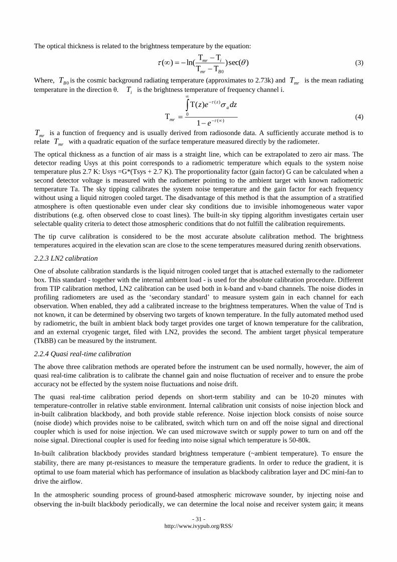
The optical thickness is related to the brightness temperature by the equation:

)sec()ln()(0

Bmr

imr

(3)

Where, 0BT is the cosmic background radiating temperature (approximates to 2.73k) and mrT is the mean radiating

temperature in the direction θ. iT is the brightness temperature of frequency channel i.

)(

0

)(

1

)(

e

dzez a

z

mr (4)

mrT is a function of frequency and is usually derived from radiosonde data. A sufficiently accurate method is to

relate mrT with a quadratic equation of the surface temperature measured directly by the radiometer.

The optical thickness as a function of air mass is a straight line, which can be extrapolated to zero air mass. The

detector reading Usys at this point corresponds to a radiometric temperature which equals to the system noise

temperature plus 2.7 K: Usys =G*(Tsys + 2.7 K). The proportionality factor (gain factor) G can be calculated when a

second detector voltage is measured with the radiometer pointing to the ambient target with known radiometric

temperature Ta. The sky tipping calibrates the system noise temperature and the gain factor for each frequency

without using a liquid nitrogen cooled target. The disadvantage of this method is that the assumption of a stratified

atmosphere is often questionable even under clear sky conditions due to invisible inhomogeneous water vapor

distributions (e.g. often observed close to coast lines). The built-in sky tipping algorithm investigates certain user

selectable quality criteria to detect those atmospheric conditions that do not fulfill the calibration requirements.

The tip curve calibration is considered to be the most accurate absolute calibration method. The brightness

temperatures acquired in the elevation scan are close to the scene temperatures measured during zenith observations.

2.2.3 LN2 calibration

One of absolute calibration standards is the liquid nitrogen cooled target that is attached externally to the radiometer

box. This standard - together with the internal ambient load - is used for the absolute calibration procedure. Different

from TIP calibration method, LN2 calibration can be used both in k-band and v-band channels. The noise diodes in

profiling radiometers are used as the „secondary standard‟ to measure system gain in each channel for each

observation. When enabled, they add a calibrated increase to the brightness temperatures. When the value of Tnd is

not known, it can be determined by observing two targets of known temperature. In the fully automated method used

by radiometric, the built in ambient black body target provides one target of known temperature for the calibration,

and an external cryogenic target, filed with LN2, provides the second. The ambient target physical temperature

(TkBB) can be measured by the instrument.

2.2.4 Quasi real-time calibration

The above three calibration methods are operated before the instrument can be used normally, however, the aim of

quasi real-time calibration is to calibrate the channel gain and noise fluctuation of receiver and to ensure the probe

accuracy not be effected by the system noise fluctuations and noise drift.

The quasi real-time calibration period depends on short-term stability and can be 10-20 minutes with

temperature-controller in relative stable environment. Internal calibration unit consists of noise injection block and

in-built calibration blackbody, and both provide stable reference. Noise injection block consists of noise source

(noise diode) which provides noise to be calibrated, switch which turn on and off the noise signal and directional

coupler which is used for noise injection. We can used microwave switch or supply power to turn on and off the

noise signal. Directional coupler is used for feeding into noise signal which temperature is 50-80k.

In-built calibration blackbody provides standard brightness temperature (~ambient temperature). To ensure the

stability, there are many pt-resistances to measure the temperature gradients. In order to reduce the gradient, it is

optimal to use foam material which has performance of insulation as blackbody calibration layer and DC mini-fan to

drive the airflow.

In the atmospheric sounding process of ground-based atmospheric microwave sounder, by injecting noise and

observing the in-built blackbody periodically, we can determine the local noise and receiver system gain; it means

- 32 -

http://www.ivypub.org/RSS/

that we can determine the calibration equation which will be used to the retrievals of atmospheric brightness

temperatures. In quasi real-time calibration, we use two-point calibration method using nonlinear correction factor,

given the observing voltages, the observing brightness temperatures can be derived using the nonlinear relationship

between in-built blackbody and blackbody with an noise injected by noise injection module.

3 SOUNDING PRINCIPLES

The integrated water vapor and liquid water content can be achieved by two-channel radiometers was demonstrated

more than two decades ago [8-9]. Typically, the atmospheric brightness temperature is measured at one frequency on

the wing of water vapor line at 23.834GHz and at a second frequency in the window region around 30GHz. The first

frequency is chose so that the water vapor absorption coefficient is nearly independent of altitude. Because the

emission of cloud liquid water increases with the frequency squared, the signal at the second frequency is dominated

by liquid water contribution. From measurements at both frequencies integrated water vapor and liquid water content

can be retrieved simultaneously [10, 11].

Recently, it has been suggested that cloud liquid water content retrievals can be improved by adding a

temperature-dependent frequency around 50 GHz [Bosisio and Mallet, 1998] or an additional frequency sensitive to

cloud liquid water at 85GHz [Bobak and Ruf, 2000]. Within this study, we will be compare the cloud liquid water

content retrieval accuracies obtained with different frequency combination obtained from ground-based

multi-frequency atmospheric microwave sounder. The chosen frequencies in this paper are 23.84GHz, 30GHz and

51.25GHz.

MPM 89 model is a broadband model for complex refractivity which is presented to predict propagation effects of

loss and delay for the neural atmosphere at frequencies up to 1000GHz. The contributions are accounted from dry air,

water vapor, suspended water droplets (haze, fog, cloud), and rain are addressed. For clear air, the local line base (44

oxygen lines and 30 water vapor lines) is complemented by an empirical water vapor continuum. Input variables are

barometric pressure, temperature, relative humidity, suspended water droplet concentration and rainfall rate.

Cruz et al. simplified MPM87 model [12] for water vapor absorption together with the improved oxygen absorption

model by Rosenkranz [13]. Refinements to the water vapor absorption model are accomplished by the addition of

three adjustable parameters, LC , WC and cC , which account for scaling of the line strength, line width and

continuum term, respectively. The oxygen absorption model is refined with the addition of the adjustable scaling

factor XC [14].

According to the comparison between MPM 89 and CRUZ model, for the chosen frequencies 23.834GHz, 30GHz

and 51.248GHz, we use CRUZ model for the first and MPM 89 model for the left two.

Figure 4 shows the atmospheric attenuation and absorption coefficients from 1 to 200 GHz, including water line

spectrum absorption, oxygen line spectrum absorption, dry-air absorption and water continuum absorption.

0 20 40 60 80 100 120 140 160 180 20010

-6

10-5

10-4

10-3

10-2

10-1

100

101

102

frequency (GHz)

abso

rptio

n（dB

/km）

US standard atmosphere, 1976

absorption-waterlines

absorption-continum

absorption-dryair

absorption-oxygen

FIG.4 THE ATMOSPHERIC ABSORPTION MODEL FROM 0-200GGHZ

- 33 -

http://www.ivypub.org/RSS/

Fig.5-6 shows the weighting function distributions for all channels of advanced multi-channel advanced

ground-based microwave radiometer calculated for a U.S. standard arctic at nadir using an atmospheric absorption

model (MPM model). The weighting functions indicate the radiative contribution of each atmospheric layer to the

measured radiance. For a given atmosphere and frequency, the peak altitude in the weighting function increases with

increasing zenith angle. This is due to increasing optical path length between the zenith and the earth when the

instruments scan from zenith to higher angles. In window channels the weighting function peaks have their

maximum closer to the surface. Most of the radiance measured by these window channels comes from the surface

and the boundary layer and these channels can be used to derive total precipitable water, precipitable rate or cloud

liquid water over ocean [15-16].

0.5 1 1.5 2 2.5 3 3.50

1

2

3

4

5

6

7

8

9

10water vapor weighting functions

weight values

heig

ht(

km

)

22.235

23.035

23.835

26.235

30.00

0 0.5 1 1.5 2 2.50

1

2

3

4

5

6

7

8

9

10temperature weighting functions

weight values

heig

ht(

km

)

51.25

52.28

53.85

54.94

56.66

57.29

58.80

FIG.5 THE WEIGHTING FUNCTIONS OF GROUND-BASED MULTI-FREQUENCY MICROWAVE SOUNDER

In Fig.6, the weighting functions of 12 channels are calculated for a U.S standard arctic atmosphere at zenith,

assuming a surface temperature of 290k, surface pressure of 1013 mbar and surface relative humidity of 70%) (a:

20-30GHz b: 50-60GHz)

FIG.6 THE WEIGHTING FUNCTIONS OF GROUND-BASED MULTI-FREQUENCY MICROWAVE SOUNDER FOR DIFFERENT ANGLES

In Fig.6, the weighting functions are calculated for a U.S standard arctic atmosphere at zenith, assuming a surface

temperature of 290k, surface pressure of 1013 mbar and surface relative humidity of 70%. The weighting functions

in different angles at 23.84GHz and 51.25 GHz, respectively.

4 CLOUD MODEL DETERMINATION

A common approach is to place clouds in a radiosonde profile, where the relative humidity exceeds a threshold of

0 0.1 0.2 0.3 0.4 0.5 0.6 0.7 0.8 0.9 10

1

2

3

4

5

6

7

8

9

10

normalized weighting functions

altitude (

km

)

54.94GHz

0 degree

20 degree

30 degree

40 degree

50 degree

60 degree

70 degree

80 degree

0 0.1 0.2 0.3 0.4 0.5 0.6 0.7 0.8 0.9 10

1

2

3

4

5

6

7

8

9

1022.235GHz

normalized weighting functions

altitude (

km

)

0 degree

20 degree

30 degree

40 degree

50 degree

60 degree

70 degree

80 degree

- 34 -

http://www.ivypub.org/RSS/

95%. Within the development of retrieval algorithms brightness temperatures based on these cloud liquid water

profiles are simulated to obtain relations between the brightness temperatures and cloud liquid water path. Generally

radiative transfer is drop size distribution dependent in the microwave region, although the drop size distribution will

only be significant at higher frequencies like 90GHz or in rainy calculations in this study, therefore the scattering is

calculated according to the MIE theory for all clouds.

4.1 Salonen cloud liquid water content model (salonen, 1991)

The following model is illustrated for a standard atmospheric profile in Fig.7 and 8.

The critical humidity Function [17]

, cU , is calculated at each altitude with the formula

)]5.0(1)[1(1 cU (5)

Where =1, 3 ,

is the ratio of the atmospheric pressure at each height to surface pressure.

Cloud is assumed to occur at each altitude where the relative humidity is greater than cU . This method is illustrated

using a simulation of a standard atmospheric profile.

FIG.7 THE CRITICAL HUMIDITY FUNCTION CALCULATED USING US STANDARD ATMOSPHERE, 1976.

FIG.8 THE CLOUD DETERMINATION USING STANDARD CRITICAL HUMIDITY FUNCTION.

4.2 Three cloud models proposed by Ulrich et al.

Ulrich Lohnert et al. presented 3 models to estimate cloud drop size distribution, like TH mode, CE method and

Dynamic cloud mode in 2003 [18]. TH method is to diagnose cloud liquid water from radiosonde measurements use

a threshold on relative humidity (RH). In Ulrich‟s study, the threshold is set by 90% or 95% thresholds, cloud layers

are taken to exist in a profile when RH exceeds the corresponding value. CE method is an alternative approach for

deriving cloud boundaries from radiosonde ascents which is a gradient method proposed by Chernykh and Eskride in

1996. A cloud is modeled into layers when it satisfies the determined conditions. Dynamic cloud model calculates

the cloud liquid water in 40 logarithmic radius classes every 250m from ground to 10km height. This convective

model was initialized with the modeling of TH mode and CE method. The disadvantage of this model is that it is

always generates clouds, and hence clear sky cases are not well represented.

4.3 The improved cloud model

In this paper, the authors combined Salonen model and TH method from Ulrich Lohnert model to detect the real

conditions happened in the train datasets and validation datasets based on the radiosonde observations. The improved

cloud model can be described as follows:

According to the humidity profiles from radiosonde datasets, first, we use equation of Salonen model to derive the

0.1 0.2 0.3 0.4 0.5 0.6 0.7 0.8 0.9 10

1

2

3

4

5

6

7

8

9

10

relative humidity

altitude (

km

)critical humidity function

RH profile

0.7 0.75 0.8 0.85 0.9 0.95 10

1

2

3

4

5

6

7

8

9

10

relative humidity

altitude (

km

)

US standard atmosphere ,1976

critical cloud function

- 35 -

http://www.ivypub.org/RSS/

critical humidity function at each discrete altitude and judge the height value where relative humidity value is larger

than critical humidity function value, then record the relative humidity value of cloud base and cloud top and judge

the relationship among them and humidity threshold from TH model. Second, using TH model and Salonen model to

derive cloud distribution, respectively. Where cloud occurs, the cloud liquid water content, w (g/m3), as a function of

temperature t (degree), and height from cloud base, is given by

)())(1(0 tPh

hctww w

r

c (6)

Whrer, a=1.4 is the parameter for height dependence. c=0.041/oC is the parameter for temperature

dependence. 0w =0.14 g/m3 is the liquid water content, if rc hh =1.5km at 0

oC. (i.e. at cloud base), )(tPw is the

liquid water fraction, approximated by

)(tPw =1 if 0 oC<t (7)

)(tPw =1+20/t if -20 o

C<t<0 oC (8)

)(tPw =0 if t< -20

oC (9)

Third, according to different cloud liquid water content calculated by different cloud estimated models, calculate

atmospheric absorption coefficients and then using microwave radiative transfer equation to simulate brightness

temperatures, comparing the simulations and observation brightness temperature from ground-based atmospheric

microwave sounder, we can judge the better model which the brightness temperatures are well agreement with the

observations. At last, in the same station, using the better cloud model, this paper calculates all the radiosonde

datasets which will be used in training, testing and validating process of ANN retrievals.

4.4 Determine the cloud layers using the infrared sensor

Although the mean cloud liquid temperature is difficult to measure directly, it may be approximated by the cloud

base temperature and measured with an infrared sensor (HBIR5816) which is operated on the top platform of

ground-based multi-frequency microwave radiometer. Its distance coefficient ratio is 50 to 1; measuring range is -32

to 50oC. This approximation works well for single-layer clouds that are sufficiently thin that their average

temperature is close to the base temperature.

For thin clouds conditions, the mean temperature is close to the base temperature, for sufficiently thick clouds, its

average temperature is significantly less than its base temperature, so the integrated cloud liquid water will be

over-estimated. The situation is worse when there are multiple cloud layers are happened and significant liquid water

exists in the upper layers. Then we need a correction model which assuming an adiabatic liquid water distribution

and pseudo-adiabatic temperature distribution within the cloud. Through this, the model reduces the effect of

multiple cloud layers and the effect of finite cloud thickness. For large amount water vapor, the infrared temperature

will be warmer than the actual cloud base temperature due to a contribution of water vapor emission.

5 INTEGRATED WATER VAPOR AND CLOUD LIQUID WATER CONTENT

Integrated water vapor and cloud liquid water content in the atmosphere can cause microwave refraction, scattering

and attenuation. Therefore, the retrieval of integrated water vapor and cloud liquid water content play a key role in

the detection of radar, aviation security and mobile satellite communications and other fields. Also it can be used in

artificial rainfall, weather forecast and number weather modification.

The atmospheric opacity, , at the measured microwave frequencies is due to the sum of a dry contribution, dry ,

from far wing of the 60GHz oxygen band, a contribution, vap , from the water vapor resonance centered at 22GHz,

and (from cloudy conditions) a contribution, liq from liquid water:

liqvapdry (10)

Vkv a pv a p (11)

Lkliqliq (12)

- 36 -

http://www.ivypub.org/RSS/

vapk , liqk are the frequency-dependent path averaged mass absorption coefficients.

Integrated water vapor content dsV v

0 2/ mg (13)

0

VVmm (cm) (14)

Integrated Liquid water content dsLr

rl

2

1

2/ mg (15)

0

LLmm (mm) (16)

Where, 0 denotes the water vapor density，in the unit of3/ mg , 1r and 2r are heights of cloud base and cloud top,

maybe there is more than one cloud layer, so the integrated Liquid water content can be the sum of several integrants.

v and l are the water vapor density and cloud liquid water density in atmosphere at height z, the unit of

parameter ds is m, and V and L are the integrated content of water vapor and liquid water in unit valume of the

cylinder.

6 RETRIEVAL METHOD

6.1 Regression method

If the dry contribution is determined separately, it can be subtracted such that

d r y * (17)

And the three equations can be solved for the estimations of V and L:

3322110 aaaaV (18)

3322110 bbbbL (19)

Where, 1 , 2 and 3 are the opacity in three channel, 0a , 1a , 2a , 3a , 0b , 1b , 2b and 3b are the retrieval

coefficients. The subscripts 1, 2 and 3 refer to the vapor, liquid water and oxygen-sensitive frequencies 22.235GHz,

30GHz and 51.25GHz. At each frequency, the opacity is calculated from the measured sky brightness Tsky derived

from equation 17.

The water vapor coefficients, 0a , 1a , 2a , 3a , exhibit a weak dependence on surface pressure and surface temperature

and humidity. The linear relationship between opacity (brightness temperature) and water vapor density profile is

evident. So using the above three equations, we can derive the water vapor density profiles using linear regression

method.

Retrieval of the cloud liquid water content is complicated by the fact that liqk decreases exponentially as liquid

water temperature increases, and thus depends strongly on the height and thickness of the cloud. Consequently, the

liquid water retrieval coefficients, 0b , 1b , 2b and 3b , also exist a strong dependence on cloud water temperature.

Also, the nonlinear regression method can be expressed as follows:

2

24

2

1322110 aaaaaV 080706215 UaTaPaa (20)

2

24

2

1322110 bbbbbL 080706215 UbTbPbb (21)

In the above two equations, the surface temperature, humidity and pressure are added, also the square terms and

cross-terms are added.

In this paper, here we use brightness temperature in chose channels instead of atmospheric opacity to construct linear

regression model and derive the regression coefficients.

6.2. Artificial neural network

- 37 -

http://www.ivypub.org/RSS/

In recent years, back propagation artificial neural network (ANN) has been used widely and retrieved temperature

profiles with high accuracy [19, 20]

. This paper presents this method to retrieve integrated water vapor and liquid water

content to demonstrate that it‟s useful and relable compared to commonly used method: regression method. ANN is

essentially a nonlinear statistical regression between a set of predictors-in this case the observation vectors X and a

set of predictands -in this case profiles of atmospheric temperature Z. The structure of ANN shows in Fig.6. The

layers 1, 2, and 3 represent the input layer, the hidden layer, and the output layer, respectively. The neurons of the

input layer are represented by vector iX ( LX,...,XX,X 321 ), where L is the number of the input neurons. The

neurons of the middle layer are represented by vector iY ( MYYYY ,...,, 321 ), where M is the number of the hidden

neurons. The neurons of the output layer are represented by vector iZ ( NZZZZ ,...,, 321 ), where N is the number of

the output neurons.

For the thj node in the hidden layer, this can be expressed as

)(1

L

i

jiijj bxwSY (22)

Where, S denotes the sigmoid function,

)e xp (1

1)(

S (23)

Where, ijw is the weighting of the connection between the thj hidden neuron and the thi input neuron and

jb denotes the bias in the thj neuron of the hidden layer. The Purelin linear function is applied between the output

layer and the hidden layer. As a result, the output values can be arbitrary in the range [0, 1]. The neuron of the output

layer can be expressed as:

kj

M

j

jkk bYw 1

Z (24)

Where jkw is the weight of the connection between the thj hidden neuron and the thk output neuron; kb is the

bias in the thk neuron of the output layer.

7 RADIOSONDE DATASETS AND EXPERIMENT

In this paper, the authors chose one year (2008) of radiosonde profiles in Beijing (54511, 116.28o in longitude and

39.93o in latitude) at 00z and 12z. For the radiosonde datasets, they provide the profiles of temperature, pressure,

height and relative humidity and do on. Then these profiles are processed at discrete levels every 50m up to 0.5km,

every 100m up to 2km, and every 250m up tp 10km. Although the number of independent measurements is only 58

levels output, this sampling ensures the retrieval profiles can accurately represented on the fixed levels. The profiles

are then put into the radiative transfer model to synthesis the brightness temperatures as simulate values and derive

the opacity for chose channels. We calculate the oxygen absorption and water vapor absorption coefficients

according to CRUZ model and MPM 89 model. Here, the surface temperature, surface pressure and relative

humidity can be directly measured by temperature, pressure and relative humidity sensor with a bias of 0.50C, 0.3mb

and 2%. The Gaussian noises of 0.5k is added in the temperature profiles. This extends the training datasets slightly

and reduces the sensitivity of the network to noise in the data and can represent all the errors affecting the

observations.

8 RETRIEVALS OF INTEGRATED WATER VAPOR AND LIQUID WATER CONTENT

Using the above linear regression equations, according to the measurements and simulations, we can derive the

regression coefficients, and can be expressed as follows:

0 1 1 2 2( ) ( )v AP APh a a T v a T v (25)

0 1 1 2 2( ) ( )L AP APh b bT v b T v (26)

And then calculate the coefficients:

- 38 -

http://www.ivypub.org/RSS/

)(049329.0)(045409.066426.0 21 vTvTh APAPv

)(046047.0)(01074.040282.0 21 vTvTh APAPL

Using the other channel at 51.248GHz, the coefficients are:

)(035278.0)(00131.0)(012167.0459.3 321 vTvTvTh APAPAPL

)(04462.0)(11658.0)(10276.01865.4 321 vTvTvTh APAPAPV

The following retrievals are derived using three channels, which are 23.835GHz, 30GHz and 51.25GHz. From the

retrievals it can been seen that using liner regression method can have accurate integrated water vapor content

compared to radiosonde datasets, however, using ANN method the retrievals are more agreement with the

radiosonde content, like shows in Fig.10. and compared the retrievals there is a good agreement between from

regression method and from MP3000A. Based on same method, this paper compared cloud liquid water content

among regression method, ANN method and from MP3000A. Also, Fig.13 shows that compared to regression

method, ANN method can get the retrievals more agreement with retrievals form MP3000A rather than regression

method. Because there is no accurate cloud liquid water content observed by radiosonde or other instruments, so in

this paper, MP3000A liquid water retrievals are considered as standard. Therefore, the retrieval root mean square

errors between MP3000A and ANN model is only a relative value. Therefore, further comparison need to do in

future.

0 50 100 150 200 2500

1

2

3

4

5

6

7

data 0800 (2008.5-2008.12)

IWV

(cm

)

0 5 10 15 20 250

0.5

1

1.5

2

2.5

3

3.5

4

4.5

5

datasets(from 2008.5 to 2008.12)

inte

gra

ted w

ate

r vapor

(cm

)

RAOB

linear regression

ANN

FIG. 9 THE ACTUAL ATMOSPHERIC INTEGRATED WATER VAPOR CONTENT FROM 2008.5 TO 2008.12

FIG.10 THE COMPARISON OF INTEGRATED WATER VAPOR CONTENT AMONG LINEAR REGRESSION, ANN AND MP3000

INSTRUMENT IN WINTER FROM 2008.10 TO 2008.12.

0 5 10 15 20 250

1

2

3

4

5

6

24 dataset (2008.5-2008.12:0800)

inte

grat

ed w

ater

vap

or c

onte

nt （

cm）

linear regression

MP3000

FIG.11 THE COMPARISON OF INTEGRATED WATER VAPOR CONTENT RETRIEVALS BETWEEN LINEAR REGRESSION METHOD AND

MP3000 INSTRUMENT IN WINTER FROM 2008.5 TO 2008.12.

- 39 -

http://www.ivypub.org/RSS/

0 50 100 150 200 2500

0.2

0.4

0.6

0.8

1

1.2

1.4

1.6

1.8

2

data 0800 (2008.5-2008.12)

CLW

(m

m)

0 2 4 6 8 10 12 14 16 18 20-0.05

0

0.05

0.1

0.15

0.2

0.25

0.3

0.35

0.4

0.45

datasets (from 2008.5 to 2008.12)

inte

gra

ted liq

uid

wate

r vapor

conte

nt

(mm

)

MP3000

linear regression

ANN

FIG.12 THE LIQUID WATER CONTENT FROM 2008.5 TO 2008.12

FIG.13 THE COMPARISON OF LIQUID WATER CONTENT AMONG LINEAR REGRESSION METHOD, ANN METHOD AND MP3000

INSTRUMENT FROM 2008.5 TO 2008.12.

9 CONCLUSION AND ANALYSIS

The performance of the advanced multi-channel ground-based microwave radiometer has the facility to provide

approximated time series measurements of integrated water vapor content and liquid water content. The instrument

has proven to be durable and reliable in continuous field observation. Also, this paper demonstrates that nonlinear

correction process is also very important to get brightness temperatures which are more agreement with the actual

theory values. Tipping and liquid nitrogen calibration in 20-30 and 50-60GHz are proper and can ensure that system

resolution and noise are in the acceptable level. Using regression method and artificial neural network, the retrievals

are reflect the various of integrated water vapor and liquid water content in time series. And compared to regression

method, ANN retrievals are more agreement with the radiosonde or MP3000A with smaller root mean square error

(the retrieval root mean square error of integrated water vapor and liquid water content are 0.0475 cm and 0.5mm,

respectively).

ACKNOWLEDGEMENTS

The work presented in this paper was sponsored by the China Meteorological Administration nonprofit sector

(meteorology) special research and grant Nos. GYHY200906035 and grant Nos. 863 High-Techs 2007AA120701.

REFERENCES

[1] HE Jieying, ZHANG Shengwei，ZhangYu. The Primary Design of Advanced Ground-based Atmospheric Microwave Sounder and

Retrieval of Physical Parameters[J], Journal Quantitative Spectroscopy & Radiative Transfer (JQSRT), volume 112, 2011,

pp:236-246

[2] MP-Series Microwave Profilers, Operating Manual, Radiometrics Corporation; 2008. http://www.radiometrics.com/MP_

Specifications_7-3-07.pdf

[3] RPG-150-90 / RPG-DP150-90 High Sensitivity LWP Radiometers. RPG‟s Atmospheric Remote Sensing Radiometers, Operating

Manual. Radiometer Physics GmbH, Version 7.50; 2008. http://www.radiometer-physics.com.

[4] Jansssen Michael A. Atmospheric remote sensing by microwave radiometry. A Wiley-interscience publication; 1995.

[5] HAN Yong and Ed R. Westwater. Analysis and improvement of tipping calibration for ground-based microwave radiometers, IEEE

transactions on geoscience and remote sensing, vol. 38, No. 3, 2000

[6] D. S. Song, K. Zhao and Z. Guan. Tipping calibration for digital gain compensative microwave radiometer and correction on antenna

sidelobe influences [J], RADIO SCIENCE, vol. 43, 2008

[7] Decker, M.T. and J.A. Schroeder. Calibration of ground-based microwave radiometers for atmospheric remote sensing. NOAA tech

momo ERL EPL-197, 1991

[8] Microwave radiometer measurements at Chilbolton liquid water path algorithm development and accuracy

- 40 -

http://www.ivypub.org/RSS/

[9] J.C. Liljegren. Two channel microwave radiometer for observations of total column precipitable water vapor and cloud liquid water

path. Fifth symposium on global change studies, Nashville, 1994, pp:262-269

[10] Westerwater, E.R. Ground-based microwave remote sensing of meteorological variables. Remote sensing by microwave radiometry,

M.A.Janssen, ed. John willy &sons, 1993

[11] Hogg, D.C., F.O. Guiraud, J.B. Snider, M.T. Decker and E.R. Westwater. A seerable dual-channel microwave radiometer for

measurement of water vapor and and liquid in the troposphere. Journal of applied meteorology, 22, 1983, pp: 789-806

[12] H. J. Liebe. MPM -- An atmospheric millimeter-wave propagation model. International Journal of Infrared and Millimeter Waves

1989; 10( 6): 631-650

[13] Rosenkranz, P. W. Absorption of Microwaves by Atmospheric Gases. Atmospheric Remote Sensing by Microwave Radiometry,

Chapter 2, Janssen MA editor, Wiley, New York, 1993

[14] Standra L. Cruz Pol, Christopher S. Ruf. Improved 20-32GHz atmospheric microwave absorption [J], Radio science, 22, 1998,

pp:1393-1333

[15] F. Ulaby, R. Moore, A Fung. Microwave remote sensing: active and passive-volume III: passive microwave sensing of the

atmosphere. Arench house,1986, pp:1282-1378

[16] Rosenkranz, P. W., Komichak M.J. and Staelin D.H. A method for estimation of atmospheric water vapor profiles by microwave

radiometry. Journal of applied meteorology, volume 21, 1982, pp: 1364-1370

[17] Salonen, E. New prediction method of cloud attenuation. Electronics letters, vol. 27, No.12, 1991, pp: 1108-1108

[18] Ulrich Lohnert and Susanne Crewell. Accuracy of cloud liquid water path from ground-based microwave radiometer [J]. Radio

science, Vol 38, No. 3, 8041.2003.5

[19] Yao Zhigang, CHEN Hongbin and LIN Longfu. Retrieving Atmospheric Temperature Profiles from AMSU-A data with Neural

Networks. Advances in Atmospheric Sciences 2005, 22(4): 606-616.

[20] Lei Shi. Retrieval of Atmospheric Temperature Profiles from AMSU-A Measurement Using Neural Network Approach. Journal of

Atmospheric and Oceanic Technology 2001, 18(3):340-347

AUTHORS

Jieying HE Research Assistant of CAS key laboratory of microwave remote sensing, National space science

center, Chinese Academy of Sciences (CAS), and get Doctor degree of philosophy (CAS key laboratory of

microwave remote sensing, National space science center, Chinese Academy of Sciences, Beijing) in 2012, now

the researching fields are microwave Remote Sensing, Atmospheric radiative transfer theory, Ground-based

microwave radiometer calibration theory and Temperature and humidity retrievals based on Satellite-based and

ground-based microwave radiometer.