1 THE INCOME ELASTICITY GAP AND ITS IMPLICATIONS FOR ECONOMIC GROWTH AND TOURISM DEVELOPMENT: THE BALEARIC VS THE CANARY ISLANDS Federico Inchausti-Sintes Universidad de Las Palmas de Gran Canaria Facultad de Economía, Empresa y Turismo. D.2.15 35017 Las Palmas de Gran Canaria, Spain. [email protected]Augusto Voltes-Dorta University of Edinburgh Business School Management Science and Business Economics Group EH8 9JS Edin burgh, United Kingdom [email protected]Pere Suau-Sanchez Universitat Oberta de Catalunya, School of Business and Economics, Av. Tibidabo, 39-43, 08035 Barcelona, Spain and Cranfield University, Centre for Air Transport Management, Martell House, University Way, Cranfield, MK43 0TR, UK [email protected]Inchausti-Sintes, F.; Voltes-Dorta, A.; Suau-Sánchez, P. (2020): "The income elasticity gap and its implications for economic growth and tourism development: the Balearic vs the Canary Islands". Current Issues in Tourism [10.1080/13683500.2020.1722618] ABSTRACT The Balearic and the Canary Islands are two well-known tourism-led economies. They both experienced a tourism boom during the same decades, and, hence, they developed a similar productive-mix. Nevertheless, there are strong economic differences between the two regions. While the Balearic Islands enjoy a high GDP per capita, the Canary Islands show a more modest performance. The results of a panel data regression confirm our hypothesis that they differ substantially in terms of income elasticity of tourism. It is two times higher in the Balearic Islands than in the Canaries, which indicates the first is perceived as a more luxurious destination. Furthermore, the results of a dynamic computable general equilibrium model show that the Canaries would converge in GDP per capita with the Balearic Islands if they attracted tourists with a similar profile as the latter. Keywords: Income elasticity; economic growth; tourism-led economies; dynamic computable general equilibrium.
Transcript
1
THE INCOME ELASTICITY GAP AND ITS IMPLICATIONS FOR ECONOMIC
GROWTH AND TOURISM DEVELOPMENT: THE BALEARIC VS THE CANARY
ISLANDS
Federico Inchausti-Sintes Universidad de Las Palmas de Gran Canaria
Facultad de Economía, Empresa y Turismo. D.2.15 35017 Las Palmas de Gran Canaria, Spain.
Universitat Oberta de Catalunya, School of Business and Economics, Av. Tibidabo, 39-43, 08035 Barcelona, Spain and
Cranfield University, Centre for Air Transport Management, Martell House, University Way, Cranfield, MK43 0TR, UK [email protected]
Inchausti-Sintes, F.; Voltes-Dorta, A.; Suau-Sánchez, P. (2020): "The income elasticity gap and its implications for economic growth and tourism development: the Balearic vs the Canary Islands". Current Issues in Tourism [10.1080/13683500.2020.1722618]
ABSTRACT
The Balearic and the Canary Islands are two well-known tourism-led economies. They both
experienced a tourism boom during the same decades, and, hence, they developed a similar
productive-mix. Nevertheless, there are strong economic differences between the two regions. While
the Balearic Islands enjoy a high GDP per capita, the Canary Islands show a more modest
performance. The results of a panel data regression confirm our hypothesis that they differ
substantially in terms of income elasticity of tourism. It is two times higher in the Balearic Islands
than in the Canaries, which indicates the first is perceived as a more luxurious destination.
Furthermore, the results of a dynamic computable general equilibrium model show that the Canaries
would converge in GDP per capita with the Balearic Islands if they attracted tourists with a similar
profile as the latter.
Keywords: Income elasticity; economic growth; tourism-led economies; dynamic computable general equilibrium.
e805814
Text Box
Current Issues in Tourism, Volume 24, Issue 1, 2021, pp. 98-116 DOI:10.1080/13683500.2020.1722618
e805814
Text Box
Published by Taylor and Francis. This is the Author Accepted Manuscript issued with: Creative Commons Attribution Non-Commercial License (CC:BY:NC 4.0). The final published version (version of record) is available online at DOI:10.1080/13683500.2020.1722618. Please refer to any applicable publisher terms of use.
2
1. INTRODUCTION
Before the 1960s, the Canary and the Balearic Islands had different economic patterns. The former
was an agriculture-led economy with a strong export orientation (Millares, Millares, Quintana &
Suárez, 2011). In 1852, the the ‘free port law’ was approved, which sought to promote the
industrialization of the Canary Islands. The law helped to boost both trade and the economy; but the
industrialization never happened (Bergasa & González-Viéitez, 1969). On the contrary, the Balearic
Islands has historicaly shown better economic performance. By 1800, the archipelago already
enjoyed a high literacy rate and a GDP per capita comparable with the richest Spanish regions
(Manera, 2006). The industrial sector represented an important share of the regional economy (24%)
during the XIX century, even though it was mainly focused on low value-added products with low
salaries and technological development (Manera & Parejo, 2012; and Manera, 2006). However, the
advent of tourism during the 1960s and ‘70s led to a strong change in the productive mix of both
archipelagos. Since that time, tourism has been, by far, the real motor of economic growth. For
instance, by 1975, the service sector represented 68.1% of the Balearic economy (Alcaide, 2003).
Indeed, the rise in tourism activity has produced a redistribution of resources from industry to
services (Copeland, 1991). According to Capó, Riera, and Rosselló (2007) and Inchausti-Sintes
(2015), this ‘de-industrialization’ is a consequence of the nature of tourism, which erodes traditional
exporting sectors. The first study distinguishes two key periods that explain this trend: first, the
tourism boom between 1965 and 1974, when the GDP grew 6.4% and 7.3% for the Balearic and the
Canary Islands, respectively, and with capital accumulation explaining more than a half of this
growth. The second key period took place between 1995 and 2000, as the trend reversed and
employment became the main source of economic growth. The consequent reduction in capital
intensity lead to a productivity drop in both archipelagos.
3
Nowadays, both regions are major sun-and-beach destinations in Europe. According to the Spanish
National Statistics Institute (INE), 81 million tourists visited Spain in 2019, 14 million of which
(17%) went to the Canary and Balearic Islands. Both archipelagos have shown similar levels of
human development in the last decades (Herrero, Soler & Villar, 2012). However, the differences in
economic performance still remain (see Figure 1 left). While the Balearics enjoy above-average
levels of GDP per capita, the Canary Islands are 18% below the national average in 2017. The
unemployment rate also differs (Figure 1 middle). The Balearics have an unemployment rate with
strong seasonal variation, yet still around the national average. On the contrary, the Canary Islands
are always above the national average. In terms of productivity, between 2008 and 2014, the tourism
sector and its associated employment in the Balearic Islands represent 42% and 29% of the GDP,
respectively. The same measures for the Canary Islands are 29% and 33% (Exceltur, 2015). Thus,
the Balearics obtain a higher tourism outcome with less labor. A possible reason is that, while the
Canaries experience a higher expenditure per international visitor, stays in the Balearics are, on
average, shorter in duration and this translates into higher average daily expenditure in peak season
(Figure 1, right). Further evidence of the strength of the Balearic tourism sector can be found when
looking at the level of foreign investment. According to the Spanish Institute for Foreign Trade
(ICEX), between 1993 and 2018, companies based in the Balearics accumulate 2.2 billion euro in
global investments in the accommodation sector, which is 8.41 times higher than the ones made by
Canarian firms. The income generated by such investments also contributes to the economic gap
between both tourism-led economies.
[Table 1 about here]
[Figure 1 about here]
4
We hypothesize that a difference in the income elasticity of inbound tourism must exist in order to
explain the broad gap in economic performance between the two regions. This intuition is supported
by past studies that have established a positive correlation between income per capita, income
elasticity and exports (Bahmani-Oskooee & Kara, 2005; Fieler, 2011; Weldemicael, 2014; or Cherif,
Hasanov & Zhu, 2016). In economic terms, a higher income elasticity implies a higher willingness to
pay as income grows, which, in turn, increases the possibilities of higher valued-added gains,
especially in service-based sectors, like tourism, with a traditional lack of productivity
improvements. However, no previous study has carried out a comparative analysis of tourism income
elasticities between different regions within the same country and its consequences in term of GDP
and employment.
In order to fill this gap, we estimate the income elasticities of inbound tourism in both regions and
quantify their economic impact. To that end, we first carry out a panel data regression on a dataset of
international tourist arrivals to the Canary and Balearic Islands, disaggregated by country of origin
and island of destination, between 2012 and 2016. As expected, we find that income elasticity is
significantly higher in the Balearic Islands. Then, a dynamic computable general equilibrium (CGE)
model is used to quantify the economic differences generated by the elasticity gap. The results show
that the Canaries would converge in GDP per capita with the Balearic Islands if assuming the income
elasticity of the latter. This conclusion has direct implications in regards to the development and
promotion of the Canary Islands as a tourism destination in the future.
The remainder of this paper is structured as follows: Section 2 reviews the literature on the
estimation of income elasticities in tourism studies. Section 3 covers the process of data collection,
the panel data regression and CGE methodology. Section 4 presents the results and discusses their
main implications. Section 5 concludes with a summary of the main findings.
5
2.LITERATURE REVIEW
2.1 Income elasticity and economic growth
Sectoral differences in productivity, alongside with an income elasticity gap, have been linked to the
transition of economic activity from low value-added sectors (e.g. agriculture) toward high value-
added, technological ones (Matsuyama, 1992). This economic progress is mainly triggered by the
rise in costs (especially salaries) as a consequence of economic growth. In the long term, the
economies embarked in this transition see how the less productive labour-intensive sectors tend to be
outsourced in cheaper economies, while focusing on more productive capital-intensive ones which
allow firms to sustain higher salaries (Hoffman, 1969; Hausmann, Hwang & Rodrick, 2007 or
Ricardo, 1821). This economic transition also affects the quantity and quality of the goods traded
internationally. According to Fieler (2011), the production technologies are more diverse in goods
with higher income elasticity, which also generate a large dispersion in prices. Thus, richer countries
that are prone to produce and consume these goods, also have an incentive to trade with them. On the
contrary, developing countries focus more on goods whose technology is similar across countries. As
a result, rich countries trade among them with differentiated goods, whereas the trade with
developing countries occurs primarily with homogeneous goods. Thus, wealthy countries tend to
enjoy an export income elasticity greater, and above one, than those of developing countries
(Bahmani-Oskooee & Kara, 2005). The former also show an import income elasticity lower than the
export one. In the long term, exports will grow faster than imports, which benefits the trade balance,
reduces the potential foreign debt imbalances, and strengthens economic growth (Houthakker &
Magee, 1969; Johnson, 1958).
In term of tourism-led economies, both the strong de-industrialization and tertiarization of their
economies limit the development of highly technological sectors, meaning that the economic
6
evolution described above does not occur. Moreover, tourism, as a service-based activity, tends to
show lower productivity compared to other industrial activities (Acelus & Arozena, 1999; Fixler &
Siegel, 1999; or Nordhaus, 2001). Hence, its capacity to sustain higher salaries is seriously limited.
Finally, these economies are usually small islands located far away from their biggest markets, and
with a strong dependence on imports. Hence, the objective of achieving a favorable export-import
income elasticity ratio, as in most developed economies, is more relevant for tourism-led economies.
2.2 Income elasticity in tourism
There is broad consensus in the literature that international tourism is a luxury good (i.e. income
elasticity higher than one). This was the main result of most studies between the 60s and 80s
(reviewed by Crouch, 1992), and more recent publications (with different geographical scopes, data
sources, and methodological approaches) have confirmed this (See e.g. Algieri & Kanellopoulou,
Model closure is ensured with several additional assumptions (Hosoe, Gazawa & Hashimoto, 2010),
such as investment being driven by savings, zero government deficit, fixed global prices and foreign
savings. We also account for unemployment by means of a minimum wage constraint: 𝑤# = 𝑃BC!,#, which implies that unemployed individuals will only work if salaries (𝑤#) compensate the
opportunity cost represented by the consumer price index (𝑃BC!,#). Both models were calibrated
assuming an unemployment rate of 29% and 11.67%, for the Canary and Balearic Islands,
respectively (according to ISTAC and IBESTAT figures).
The dynamic nature of our model also requires us to define annual rates of economic growth (g),
depreciation of capital ( ), and an interest rate ( ). Economic growth is assumed at 1.6% according
to IMF (2019) and the annual depreciation rate is 5% (Escribá-Pérez, Murgui-García & Ruiz-
Tamarit, 2017). Therefore, the initial stock of capital (K0) and the interest rate are determined as
follows: K0 = Inv/(g+δ) and ir =(VK/K0)−δ. Where Inv denotes total investment and VK refers to
the total gross operating surplus.
ttourism
iv
e
d ir
19
The government and the household’s capital endowment change over time as follows:
(15)
(16) ,
where and denote the gross operating surpluses accrued by the household and the
government, respectively. And, and , denote the initial endowment of investment for
the household and the government, respectively.
Finally, we assume an annual increase of 2% in arrivals (this is the shock to be modelled), which is
the forecast established by the World Tourism Organization for Southern Europe in the following 30
years (2010-2030) (UNWTO, 2011). Therefore, we use a time horizon of 21 years in the dynamic
model (2019-2030).
4. RESULTS AND DISCUSSION
4.1 Panel-data regression
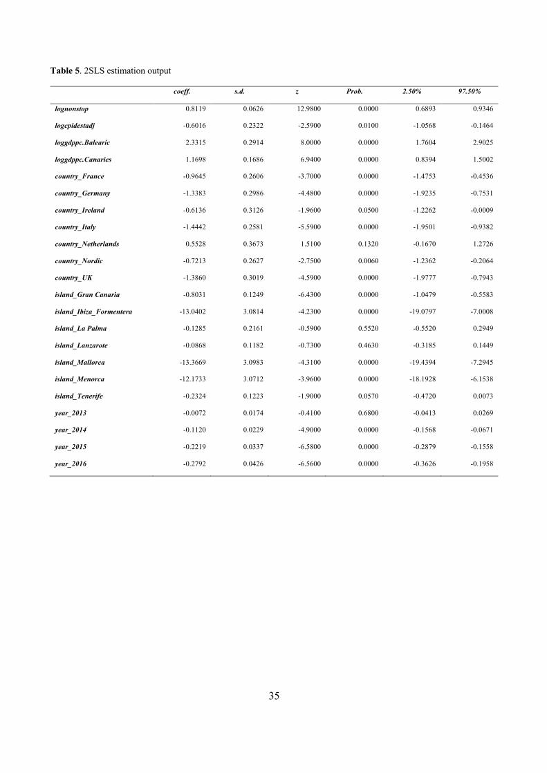
Table 5 shows the estimation results for the 2SLS regression. The coefficients of loggdppc.Balearic
and loggdppc.Canaries clearly support our working hypothesis: the Balearic Islands show a tourism
income elasticity of 2.33 which is two times higher than the respective elasticity in the Canary
Islands (1.16). This indicates the first is perceived as a more luxurious destination. According to
Peng et al (2015), the average tourism income elasticity in Europe is 2.4. The Balearic income
elasticity is around the same magnitude than the one estimated for winter tourism in Switzerland
(Falk, 2014) or Japanese tourists in New Zealand (Lim et al, 2008). On the other hand, the income
,, , 1 , 1(1 ) ( )H tH t H t H t tK K VK inv inv ird d
- -= - + + +
, 0, , 1 , 1(1 ) ( )G tG t G t G t tK K VK inv inv ird d=- -
= - + + +
,H tVK
,G tVK
, 0H tinv = , 0G tinv =
20
elasticity in the Canary Islands is closer in value to the Chinese tourist demand to Thailand (Untong
et al, 2015). Still, both values are more optimistic than the global elasticities reported by Gunter and
Smeral (2016) for the period 2004-2013, with a tourism income elasticity well below one (0.2) for
Southern Europe.
We find inbound tourism demand to be price-inelastic: a 1% increase in relative prices decreases
demand by 0.6%. This result is opposite to Crouch (1995), Garín-Muñoz (2006) and Garín-Muñoz &
Montero-Martín (2007), who all argue that sun-and-beach destinations tend to be price-elastic.
According to Peng et al. (2015), the price is also elastic for tourism in Europe (-1.20). On the other
hand, Gunter and Smeral (2016) obtained an inelastic price sensitivity, with some few exceptions, for
the period 1977-2013. For instance, price elasticity is -0.61 at world level, whereas is -0.50 for
Southern Europe.
[Table 5 about here]
[Table 5 (continue) about here]
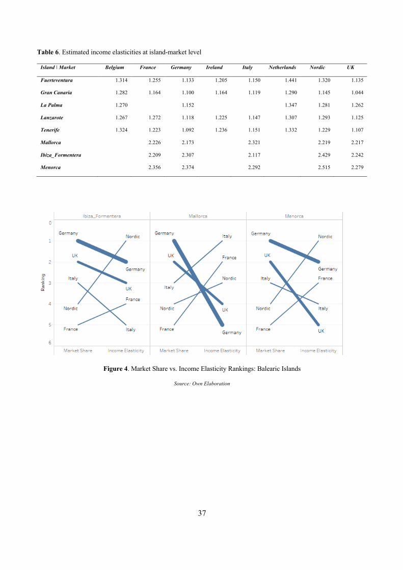
We can also disaggregate the income elasticities according to geographical market. The estimates are
shown in Table 6, and, as expected, all the Canary Islands show an income elasticity lower than the
Balearic Islands in all cases. The regional-level differences in income elasticity remain statistically
significant at 5% level. There are also differences in the central estimates of income elasticity across
the major origin countries within each region. Thus, our results point to a similar conclusion than that
of Jensen, (1998), Smeral (2003) or Smeral (2014) about the existence of different segments for
inbound tourism demand according to nationality and, hence, to the different preferences and income
levels of these visitors.
21
[Table 6 about here]
In accordance with the established interpretation of income elasticities in relation to product
positioning and market segmentation, it is possible to investigate whether the differences between the
Canary and Balearic Islands can be traced to their current market mixes. The slope graphs provided
in Figures 4 to 6 show the differences in the relative ranking of origin markets according to income
elasticity and share of visitors. Countries with a higher ranking in terms of income elasticity will
perceive the destination as more luxurious and hence, they can be considered as very attractive, non-
saturated, high-yield markets. This ranking can be compared to the actual country market shares in
each island to evaluate whether the islands are currently serving their most attractive inbound
markets. Results show that the minor Balearic Islands of Menorca, Ibiza, and Formentera have the
most distinctive visitor profiles, because their top market (Germany) is also among their most
income-elastic. This suggests a better market positioning as a luxury destination, which is seen very
clearly in the respective branding strategies developed by the local tourism boards (e.g.
www.ibizaluxurydestination.com) that reinforce aspects such as exclusivity that are highly appealing
to these visitors. The other islands, including Mallorca and all the Canaries show a different, more
traditional profile, with income elasticities and market shares showing an inverse rank correlation,
which signals a specialization on massive tourism markets with a higher degree of saturation. Thus, a
second conclusion is that the Balearics achieve better tourism outcomes because they have been able
to offer visitors a more diversified choice of destinations, with minor islands focusing on a luxury
experience while the main island retains its high-end massive appeal. In spite of that, most islands
have room for improvement by growing their most income-elastic market segments. Indeed, the
German and UK visitors to the Canary Islands show evident signs of being a mature market, while
the Netherlands, Belgium, and the Nordic Countries appear to be the best targets for further
development.
22
[Figure 4 about here]
[Figure 5 about here]
[Figure 6 about here]
4.2 CGE model
The economic consequences of the elasticity gap are quantified with a dynamic CGE model, in
which we simulate the Canaries experiencing the same tourism income elasticity than the Balearics
between 2019 and 2030. Two scenarios are presented: in Scenario A, the income elasticity affects
key tourism-related goods (“accommodation”, “catering services”, “real estate”, “rent a car”, “travel
agencies” and “entertainment”). In Scenario B, the income elasticity affects all goods. Both scenarios
are shocked by a 2% annual increase in tourism arrivals. For comparability, we simulated the same
scenarios but for the opposite case: the Balearics having the same elasticity than the Canaries
(Scenarios A* and B*).
According to Table 7, the Canaries would grow between 20% and 40% over the period in Scenarios
A and B, respectively. In total, there would be 82,596 new jobs (3,933 new annual jobs) which
would imply a reduction in the unemployment rate from 20% to 12.75% by 2030 in Scenario A. This
value is similar to the current unemployment rate in the Balearic Islands (11.67%). The estimate of
new jobs created is slightly worse in Scenario B, which can be explained by the higher prices (due to
higher GDP) that reduces the willingness to work. With their own income elasticity, the Baleric
Islands are predicted to grow between 22% and 29%, without a significant reduction in
unemploymentii.
23
[Table 7 about here]
These results can be better contextualized when translating the multiplicative GDP effects into real
values. Table 8 shows the ranking of the Spanish Autonomous Communities by GDP per capita in
2018. The Balearic Islands enjoy a GDP per capita slightly above the national average. On the
contrary, the Canary Islands are located in the lower half with a GDP per capita that is 1.22 and 1.27
times lower than the national average and the Balearic Islands, respectively. However, the
differences in GDP per capita between both archipelagos would reduce from the actual 27% to 4% in
Scenario A, and to -9% in Scenario B as the Canaries would converge in GDP per capita with the
wealthiest Spanish regions. In the opposite situation (Scenarios A* and B*), the Balearics would fall
to the lower half, closer to the Canaries’ current satiation. Thus, it is clear that, ceteris paribus, the
tourism income elasticity plays a key role in the economic performance of both insular regions. This
illustrates the benefits of transitioning towards a higher-end “luxury” destination to tap the more
income-elastic traveller segments.
[Table 8 about here]
4.3 Policy implications
Policymakers and the overall tourism sector in the Canaries should wonder about whether there is a
lack of market identification and/or service quality that prevent high-income tourists from travelling
to their destinations. At first sight, increasing the ability of tourism destinations to achieve better
outcomes clashes with the lower potential for productivity gains traditionally associated to service
activities. However, improvements can still be achieved by means of enhancing quality, which
should be a strategic cornerstone in tourism-led economies. First, local authorities can promote the
investment in better tourism infrastructure as well as in the preservation of the islands’ natural
24
resources. In relation to this, during the last decades, both regional governments have been approving
tourism moratoria laws to restrict the development of tourism accommodation supply while granting
exceptions to hotels upgrading their facilities (Hernández-Martín, Álvarez-Albelo & Padrón-Fumero,
2015).
Secondly, a detailed market analysis and segmentation based on income elasticities seems a suitable
way to identify attractive market segments and guide strategic decisions about where to invest in
destination marketing campaigns and what to advertise. In line with the more diversified choice
presented by the Balearics, these can include promotional actions at the main origin airports of the
target countries that attempt to re-brand some of the minor islands (such as Lanzarote or La Palma)
as places suitable for luxury visitors, while the major islands (Gran Canaria and Tenerife) can
continue their transition towards the high-end massive tourism market. Focusing the development of
the luxury market in the minor islands has the advantage of reduced investments and better chances
of developing a differentiated brand image with respect to the massive tourism offer in the major
islands.
5. SUMMARY
Despite the many similarities between the Balearic and the Canary Islands, a strong economic gap
exists between the two regions. We hypothesize that this gap is linked to a different market
positioning, and thus income elasticities, of the respective tourism products. In order to prove this
intuition, we carried out a panel data regression on international tourism arrivals to the Balearic and
Canary Islands between 2012 and 2016 and we estimate the economic consequences of the elasticity
gap with a CGE model.
25
The results of a panel data regression confirm our hypothesis that income elasticities differ
significantly between both regions. It is two times higher in the Balearic Islands than in the Canary
Islands, which indicates the first is perceived as a more luxurious destination. Overall, the Balearics
offer a more diversified choice of destinations, with minor islands focusing on a luxury experience
while the main island retains its high-end massive appeal. The conclusions of the GCE modelling
indicate that, if the Canaries experienced the tourism income elasticity of the Balearics, the region
will increase its GDP per capita in 22%, thus eliminating the income gap between the insular regions.
These results emphasize the importance of focusing on higher value-added tourist activities. In
tourist terms, this means investing in quality and service innovation by e.g. upgrading tourism
infrastructure while preserving the islands’ natural attributes. Such improvements can be more
effective if they are targeted to the markets with a higher perception of the tourism product on offer,
which can be identified by means of a detailed market segmentation. In the Canaries, marketing
efforts could consider re-branding some of the minor islands as luxury destinations, while the major
islands continue their transition towards high-end massive markets.
Our conclusions, however, should be interpreted with caution, as there are some limitations to our
empirical estimates. First, the sample period (2012-2016) is relatively short and inevitably impacted
by extraordinary events like the global recession, which can compromise the generalizability of our
policy implications to other periods. Unfortunately, the time-series dimension of the dataset is
defined by the availability of MIDT data that is necessary to disaggregate passenger arrivals
according to origin markets. Still, expanding the sample period further back would not have
mitigated the problem since the recession started in 2008, and the beginning of the Arab Spring in
the early 2010s can also be expected to affect the number of passenger arrivals to both regions. A
more recent time series would have allowed us to better capture the impact of the Brexit vote on UK
inbound demand, which is one of the islands’ key markets. Secondly, it is not possible to obtain
26
monthly income data for the travellers, which does not allow us to fully disaggregate the income
elasticity between peak and off-peak periods in the Balearics. This would have been of interest as
travellers’ profiles can be different across the year. Third, there is also a shortcoming in the lack of
socioeconomic indicators in the analysis (e.g. age, group size), that could also serve to illustrate the
differences between the tourism markets served by both regions. All these limitations can be
overcome as data becomes available. Further research can also investigate how and whether the
emergence of low-cost carriers in the Spanish island airports has affected the income elasticities of
inbound tourism over time, by making travel more affordable and perhaps increasing the proportion
of lower-income visitors. In view of the results of this paper, confirming that hypothesis would have
implications on the dilemma faced by local authorities between investing in service quality to attract
more high-end visitors and granting subsidies to low-cost operators to boost inbound traffic. Other
interesting areas to cover relate to how the Balearics seem to benefit from extreme seasonality,
despite the challenges traditionally associated to that characteristic of inbound traffic in the areas of
planning and management of tourism resources.
27
REFERENCES
Acelus F.J. and Arozena, P. 1999. “Measuring sectoral productivity across time and across countries”. European Journal
of Operational Research 1119 (2): 254-266.
Alcaide, J., 2003. “Evolución económica de las regiones y provincias españolas en el siglo XX”. Bilbao: Fundación BBVA.
Alegre, J., and Pou, L., 2004. “Micro-economic determinants of the probability of tourism consumption”. Tourism
Economics 10(2): 125-144.
Alegre, J., Mateo, S., and Pou, L., 2009. “Participation in tourism consumption and the intensity of participation: An
analysis of their socio-demographic and economic determinants”. Tourism Economics 15(3): 531-546.
Algieri, B., and Kanellopoulou, S., 2009. “Determinants of Demand for Exports of Tourism: An Unobserved Component
Model”. Tourism and Hospitality Research 9(1): 9-19.
Álvarez-Díaz, M., González-Gómez, M., and Otero-Giráldez, M.S., 2015. “Research note: Estimating price and income
demand elasticities for Spain separately by the major source markets”. Tourism Economics 21(5): 1103-1110.
Armington, P., S., 1969. “A theory of demand for products distinguished by place of production”. International Monetary
Fund (Staff Papers), 16(1): 159-178. Washington DC, US.
Bahmani-Oskooee, M., and Kara, O., 2005. “Income and price elasticities of trade: some new estimates”. The International
Trade Journal 19 (2): 165-178.
Bergasa. O., and González-Viéitez. A., 1969. “Desarrollo y subdesarrollo de la economía canaria”. 1ª ed. Madrid:
Guadiana.
Bernini, C., and Cracolici, M.F., 2016. “Is participation in the tourism market an opportunity for everyone? Some evidence
from Italy”. Tourism Economics 22(1): 57-79.
Blake, A., Durbarry, R., Eugenio-Martin, J. L., Gooroochurn, N., Hay, B., Lennon, J., & Yeoman, I., 2006. “Integrating
forecasting and CGE models: The case of tourism in Scotland”. Tourism Management, 27(2): 292-305.
Breusch, T. S., and Pagan, A. R., 1980. “The Lagrange multiplier test and its applications to model specification in
econometrics”. The Review of Economic Studies, 47(1): 239-253.
Cherif, R., Hasanov, F., and Zhu. M., 2016. “Breaking the oil spell: the gulf falcons´path to diversification”. Washington
DC: International Monetary Fund.
Copeland, B. R., 1991. “Tourism, welfare and de-industrialization in a small open economy”. Economica, 515-529.
Crouch, G.I., 1992. “Effect of income and price on international tourism”. Annals of Tourism Research 19(4): 643-664.
28
Dougan, J.W., 2007. “Analysis of Japanese tourist demand to Guam”. Asia Pacific Journal of Tourism Research 12(2: 79-
88.
Eugenio-Martin, J.L., and Campos-Soria, J.A., 2011. “Income and the substitution pattern between domestic and
international tourism demand”. Applied Economics 43(20): 2519-2531.
Escribá-Pérez, J., Murgui-García, M.J., & Ruiz-Tamarit, J.R., 2017. “Medición económica del capital y depreciación
endógena: una aplicación a la economía española y sus regions”. Investigaciones regionales- Journal of Regional
Research, 38: 153-180.
Exceltur., 2015. “Estudios del impacto económico del turismo sobre la economía y el empleo de las Illes Balears”.
Available at: https://www.exceltur.org/impactur/#
Falk, M., 2014. “The sensitivity of winter tourism to exchange rate changes: Evidence for the Swiss Alps”. Tourism and
Hospitality Research 13(2): 101-112.
Falk, M., and Lin, X., 2018. “Income elasticity of overnight stays over seven decades”. Tourism Economics 24(8): 1015-
1028.
Fieler, A. C., 2011. “Nonhomotheticity and bilateral trade: Evidence and a quantitative explanation”. Econometrica 79 (4):
1069-1101.
Fixler D. J., and Siegel, D., 1999. “Outsourcing and productivity growth in services”. Structural Change and Economic
Dynamics 10 (2): 177-194.
Fredman, P., and Wikström, D., 2018. “Income elasticity of demand for tourism at Fulufjället National Park”. Tourism
Economics 24(1): 51-63.
Garin-Muñoz, T., 2006. “Inbound international tourism to Canary Islands: A dynamic panel data model”. Tourism
Management, 27(2): 281-291.
Garin-Munoz, T., and Montero-Martín, L. F., 2007. “Tourism in the Balearic Islands: A dynamic model for international
demand using panel data”. Tourism Management, 28(5): 1224-1235.
González A., and Matés, J. M., 2007. “Historia económica de Esapaña”. Barcelona: Ariel.
Gunter, U., and Smeral, E., 2016. “The decline of tourism income elasticities in a global context”. Tourism Economics
22(3): 466-483.
Hausman, J., 1978. “Specification tests in econometrics”. Econometrica 46: 1251-1271.
Hausmann, R., Hwang, J., and Rodrik, D., 2007. “What you export matters”. Journal of Economic Growth, 12 (1): 1-25.
29
Hernández-Martín, R., Álvarez-Albelo, C., & Padrón-Fumero, N. 2015. “The economics and implications of moratoria on
tourism accommodation development as a rejuvenation tool in mature tourism destinations”. Journal of Sustainable
Tourism, 23 (6), 881-899.
Herrero, C., Soler, A., and Villar, A., 2013. “Desarrollo humano en España: 1980-2011”. Valencia: Ivie, 54. Available at:
http://dx.doi.org/10.12842/HDI_2012
Hoffmann, W. G., 1968. “The growth of industrial economies”. Manchester: Manchester University Press.
Hosoe, N., Gasawa, K., and Hashimoto, H., 2010. “Textbook of Computable General Equilibrium Modelling:
Programming and Simulations”. Hampshire, UK: Palgrave Macmillan.
Houthakker, H. S., and Magee, S. P., 1969. “Income and price elasticities in world trade”. The review of Economics and
Statistics, 111-125.
Inchausti-Sintes, F., 2015. “Tourism: Economic growth, employment and Dutch disease”. Annals of Tourism Research,
Figure 4. Market Share vs. Income Elasticity Rankings: Balearic Islands
Source: Own Elaboration
38
Figure 5. Market Share vs. Income Elasticity Rankings: Eastern Canary Islands
Source: Own Elaboration
Figure 6. Market Share vs. Income Elasticity Rankings: Western Canary Islands
Source: Own Elaboration
39
Table 7. Annual change in GDP, Unemployment and inflation in the Canary Islands (2019-2030).
Scenario A Scenario B
Canaries Balearics Canaries Balearics
GDP multiplier (GDP2.33/ GDP1.66) 1.22 1.22 1.40 1.29
Unemployment (%) 1.70% - 1.58% -
New Jobs 3,933 - 3,625 -
40
Table 8. Ranking of the Spanish autonomous communities by GPD per capita (euros), 2018.
Autonomous Community GDP per capita
Community of Madrid 34,916
Basque Country 34,079
Navarre 31,809
Catalonia 30,769
Canary Islands (Scenario B) 29,443
Aragon 28,640
La Rioja 26,833
Balearic Islands 26,764
National average 25,854
Canary Islands (Scenario A) 25,657
Castile y Leon 24,397
Cantabria 23,817
Galicia 23,294
Asturias 23,087
Valencian community 22,659
Balearic Islands (Scenario A*) 21,937
Region of Murcia 21,134
Canary Islands 21,031
Balearic Islands (Scenario B*) 20,747
Castile-La Mancha 20,645
Ceuta 20,032
Andalusia 19,132
Melilla 18,482
Extremadura 18,174
Source: INE.es, Own elaboration
i Historical exchange rates are sourced from http://xe.com. ii According to our model, the Balearics require an annual increase in arrivals of 4% to reduce unemployment.