Brigham Young University Brigham Young University BYU ScholarsArchive BYU ScholarsArchive Theses and Dissertations 2016-02-01 The Influence of Season, Heating Mode and Slope Angle on The Influence of Season, Heating Mode and Slope Angle on Wildland Fire Behavior Wildland Fire Behavior Jonathan R. Gallacher Brigham Young University - Provo Follow this and additional works at: https://scholarsarchive.byu.edu/etd BYU ScholarsArchive Citation BYU ScholarsArchive Citation Gallacher, Jonathan R., "The Influence of Season, Heating Mode and Slope Angle on Wildland Fire Behavior" (2016). Theses and Dissertations. 5691. https://scholarsarchive.byu.edu/etd/5691 This Dissertation is brought to you for free and open access by BYU ScholarsArchive. It has been accepted for inclusion in Theses and Dissertations by an authorized administrator of BYU ScholarsArchive. For more information, please contact [email protected], [email protected].
Transcript
Brigham Young University Brigham Young University
BYU ScholarsArchive BYU ScholarsArchive
Theses and Dissertations
2016-02-01
The Influence of Season, Heating Mode and Slope Angle on The Influence of Season, Heating Mode and Slope Angle on
Wildland Fire Behavior Wildland Fire Behavior
Jonathan R. Gallacher Brigham Young University - Provo
Follow this and additional works at: https://scholarsarchive.byu.edu/etd
BYU ScholarsArchive Citation BYU ScholarsArchive Citation Gallacher, Jonathan R., "The Influence of Season, Heating Mode and Slope Angle on Wildland Fire Behavior" (2016). Theses and Dissertations. 5691. https://scholarsarchive.byu.edu/etd/5691
This Dissertation is brought to you for free and open access by BYU ScholarsArchive. It has been accepted for inclusion in Theses and Dissertations by an authorized administrator of BYU ScholarsArchive. For more information, please contact [email protected], [email protected].
The Influence of Season, Heating Mode and Slope Angle on Wildland Fire Behavior
Jonathan Ray Gallacher Department of Chemical Engineering, BYU
Doctor of Philosophy
Wildland fire behavior research in the last 100 years has largely focused on understanding the physical phenomena behind fire spread and on developing models that can predict fire behavior. Research advances in the areas of live-fuel combustion and combustion modeling have highlighted several weaknesses in the current approach to fire research. Some of those areas include poor characterization of solid fuels in combustion modeling, a lack of understanding of the dominant heat transfer mechanisms in fire spread, a lack of understanding regarding the theory of live-fuel combustion, and a lack of understanding regarding the behavior of flames near slopes.
In this work, the physical properties, chemical properties and burning behavior of the foliage from ten live shrub and conifer fuels were measured throughout a one-year period. Burn experiments were performed using different heating modes, namely convection-only, radiation-only and combined convection and radiation. Models to predict the physical properties and burning behavior were developed and reported. The flame behavior and associated heat flux from fires near slopes were also measured. Several important conclusions are evident from analysis of the data, namely (1) seasonal variability of the measured physical properties was found to be adequately explained without the use of a seasonal parameter. (2) ignition and burning behavior cannot be described using single-parameter correlations similar to those used for dead fuels, (3) moisture content, sample mass, apparent density (broad-leaf species), surface area (broad-leaf), sample width (needle species) and stem diameter (needle) were identified as the most important predictors of fire behavior in live fuels, (4) volatiles content, ether extractives, and ash content were not significant predictors of fire behavior under the conditions studied, (5) broadleaf species experienced a significant increase in burning rate when convection and radiation were used together compared to convection alone while needle species showed no significant difference between convection-only and convection combined with radiation, (6) there is no practical difference between heating modes from the perspective of the solid—it is only the amount of energy absorbed and the resulting solid temperature that matter, and (7) a radiant flux of 50 kW m-2 alone was not sufficient to ignite the fuel sample under experimental conditions used in this research, (8) the average flame tilt angle at which the behavior of a flame near a slope deviated from the behavior of a flame on flat ground was between 20° and 40°, depending on the criteria used, and (9) the traditional view of safe separation distance for a safety zone as the distance from the flame base is inadequate for fires near slopes.
Keywords: physical properties, live fuels, fuel growth patterns, ignition, fire behavior, seasonal burning behavior, radiation, convection, Coanda effect, fire attachment on slopes, safe separation distance, firefighter safety zone
ACKNOWLEDGEMENTS
I thank my research advisor, Tom Fletcher, for his guidance, mentorship, motivation and
support while completing this project. I acknowledge his effort in walking the line between
teaching effective research skills and allowing me to grow through experience. I am thankful for
his help and friendship on a personal and professional level. I am grateful to David Weise for his
mentorship and for his willingness to share his vast knowledge in all areas of wildland fire, all
while continuing his work at the Pacific Southwest Research Station in Riverside, CA. I thank
the other members of my graduate committee, David Lignell, Vince Wilding and Brad Bundy,
for their feedback and support.
I am grateful for the efforts of those who collected samples and sent them to our lab: Joey
Chong, Gloria Burke and Bonni Corcoran from Riverside, CA; Scott Pokswinski from Newton,
GA; and Sara McAllister, Matt Jolly and Rachael Kropp from Missoula, MT. I am grateful for
the collaboration with faculty and students from the University of Alabama – Huntsville: Babak
Shotorban, Bangalore Yashwanth, Shankar Mahalingam and Selina Ferguson. I am grateful to
the many undergraduate students from BYU who helped with this project: Victoria Lansinger,
Sydney Hansen, Samantha Smith, Kelly Wilson, Ashley Doll, Taylor Ellsworth, Kristen
Nicholes, Marianne Fletcher, Aaron Bush, Timothy Snow and Colton Hickman. This project
would not have been possible without the work of all the people mentioned herein. I note with
special thanks the contributions of Victoria Lansinger and Sydney Hansen for the work they put
in while I was busy with course work and the department qualifying exam. I also acknowledge
the work of Devin Kimball and Brad Ripa in performing experiments to study the Coanda
Effect.
I am grateful for the collaboration and friendship of other graduate students, namely
Dallan Prince, Chen Shen, Robert Laycock, Aaron Lewis, He Yang and Dan Jack. I am also
grateful for mentoring from other experts in the field of fire research, specifically Sara
McAllister, Bret Butler and Mark Finney from the Missoula Fire Lab in Missoula, MT.
I acknowledge the support and encouragement I received from my family, particularly
from my parents and my wife’s parents. I thank my children, Rachel, Caleb and Spencer, whose
happiness and excitement brightened many weary days. I especially thank my wife, Kiera, for
being a rock of support, comfort and love. I also thank her for her patience in following me
across the country to complete graduate school. Lastly, I thank my Heavenly Father and His
son, Jesus Christ, for guidance from the Holy Ghost and for the chance to repent and change for
the better.
This work was supported by Joint Fire Sciences Program (JFSP) Grant 11-1-4-14 through
United States Department of Agriculture (USDA) Forest Service Pacific Southwest (PSW)
Research Station agreement 11-JV-11272167-044 and Brigham Young University. Any opinions,
findings, and conclusions or recommendations expressed in this dissertation are those of the
graduate student and advisor and do not necessarily reflect the views of the JFSP or any other
government funding agency.
v
TABLE OF CONTENTS
List of Tables viii
List of Figures x
1 Introduction 1
2 Literature Review 4
Fuel Element Property Measurements and Modeling 4
Ignition and Burning of Wildland Fuels 8
2.2.1 Ignition Time and Temperature 8
2.2.2 Effect of Moisture on Ignition Characteristics and the Differences between Live and Dead Fuels 10
2.2.3 Effect of Heat Transfer Mode on Ignition 13
2.2.4 Ignition Summary 15
Wildland Fire Modeling 16
2.3.1 Statistical Models 17
2.3.2 Physical Models 17
2.3.3 Empirical Models 19
2.3.4 Simulation Models 21
2.3.5 Modeling Summary 22
Fire Fighter Safety Considerations 23
2.4.1 Current Safety Zone Models 24
2.4.2 The Coanda Effect and its Influence on Fire Behavior near Solid Surfaces 25
2.4.3 The Coanda Effect and Safety Zones 26
Summary 27
3 Objective and Tasks 28
Objective 28
Tasks 28
4 Physical Properties and Dimensions for Ten Shrub and Confier Fuels to Predict Fire Behavior 30
Methods 30
4.1.1 Measurements 30
4.1.2 Physical Properties Model Development 37
Results and Discussion 41
vi
4.2.1 Size and Shape Measurements 41
4.2.2 Chemical Composition Measurements 46
4.2.3 Dry Mass Distribution 48
4.2.4 Prediction Models 50
4.2.5 Uncertainty Analysis 54
Summary and Conclusions 58
5 The Effect of Heating Mode on Ignition and Burning of Ten Live Fuel Species 60
Methods 60
5.1.1 Experiment Description 60
5.1.2 Analysis of Heat Transfer Conditions 64
Results and Discussion 66
Summary and Conclusions 73
6 Seasonal Changes in Ignition and Burning of Live Fuels using Natural Variation in Fuel Characteristics 75
Methods 75
6.1.1 Experimental Setup 75
6.1.2 Model Development 76
Results and Discussion 77
6.2.1 Effects of Sample Condition, Season, Moisture Content and Species 77
6.2.2 Single Variable Regressions 82
6.2.3 Multi-variable Regressions 85
6.2.4 Uncertainty Analysis 98
Summary and Conclusions 100
7 The Influence of the Coanda Effect on Flame Attachment to Slopes and Firefighter Safety Zone Considerations 102
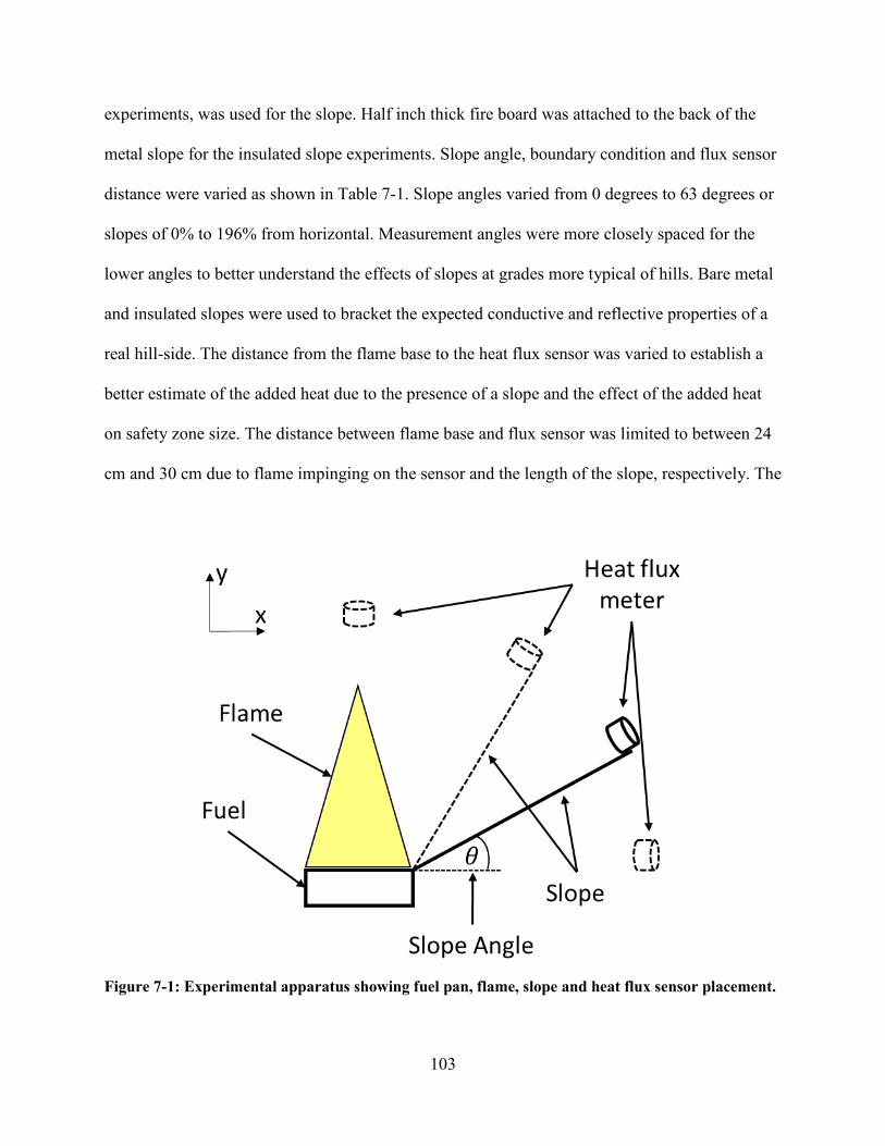
Methods 102
Results 107
7.2.1 Flame Behavior Measurement Results 108
7.2.2 Heat Flux Measurement Results 111
7.2.3 Dimensional Analysis 116
Discussion 124
Summary and Conclusions 126
8 Summary and Conclusions 128
vii
Physical and Chemical Properties 128
The Effects of Heating Mode on Ignition 128
Seasonal Variations in Ignition and Burning Behavior 129
The Effect of Slope Angle on Fire Behavior 130
Recommended Future Work 132
References 134
Appendix 151
A. Preliminary Riverside Results 152
1 Introduction 152
2 Experimental Methods 153
A. 2.1 Shrub Combustion Experiment 153
A. 2.2 Individual Leaf Combustion Experiment 155
3 Shrub Combustion Modeling 156
4 Results and Discussion 159
A. 4.1 Shrub Combustion Experiments 159
A. 4.2 Shrub Combustion Modeling 162
5 Future Work 164
6 Conclusions 164
7 Acknowledgements 165
B. Prediction Model Parity Plots 166
Physical Properties Models 166
Ignition and Burning Behavior Models—Best Overall Models 173
Ignition and Burning Behavior Models—Models Using Most Common Parameters 181
C. Experimental Data 189
Physical and Chemical Properties Data 189
Ignition and Burning Data 189
Temperature Plateau Data 190
Data for Flame Behavior near Slopes 191
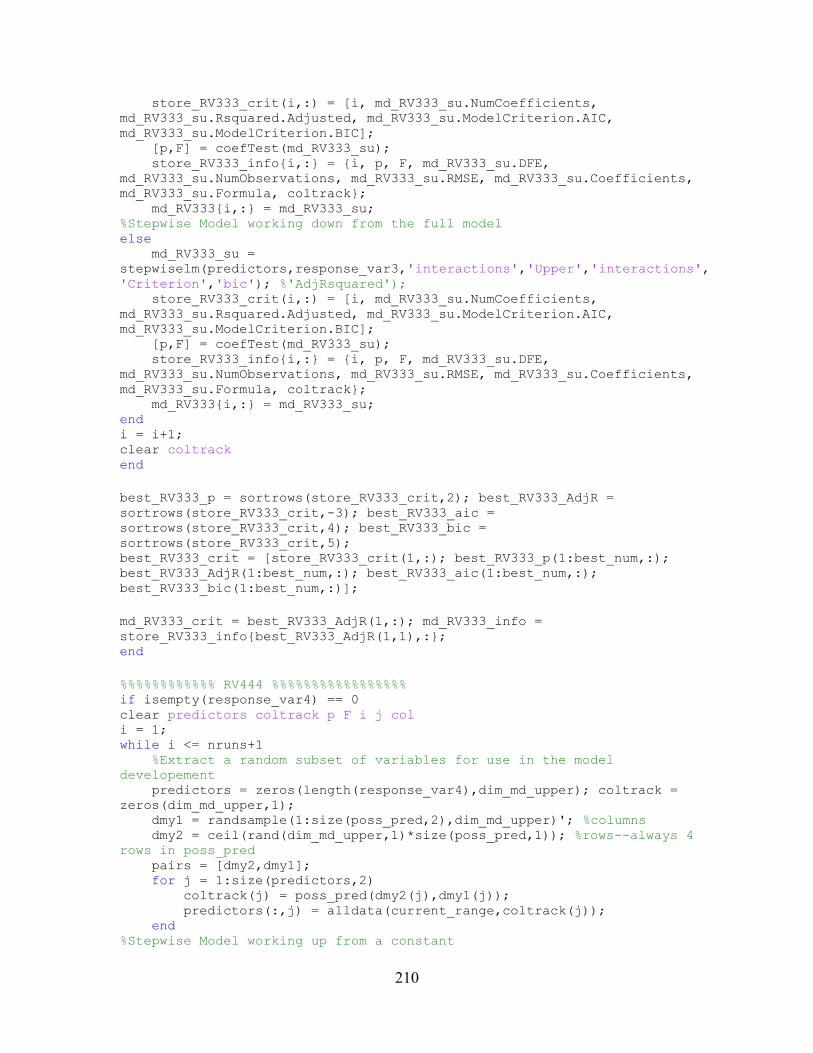
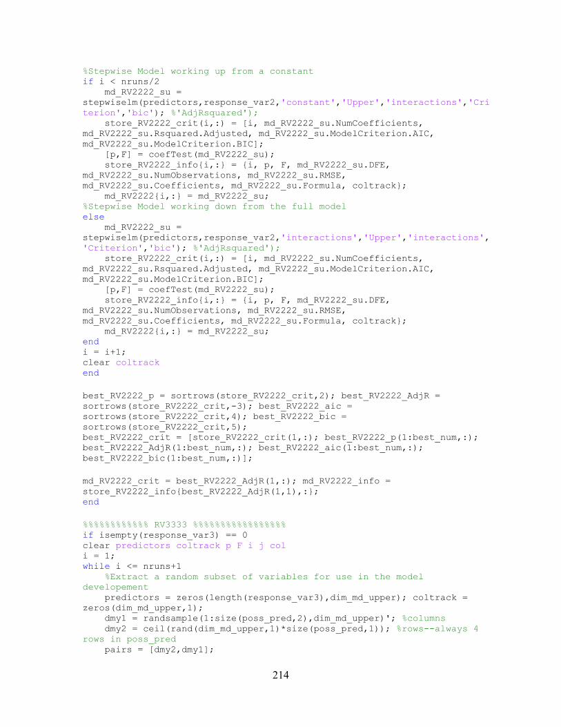
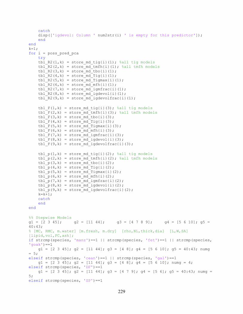
D. Data Processing and Model Development Algorithms 192
Surface Area Measurement Algorithm 192
Physical Properties Model Development Algorithm 193
Ignition and Burning Model Development Algorithm 217
viii
LIST OF TABLES
Table 4-1: Measurement definitions 32 Table 4-2: Species tested. 33 Table 4-3: Yearly average and standard deviation for measured foliage characteristics—
broadleaf species. 43 Table 4-4: Yearly average and standard deviation for measured foliage characteristics—
needle species. 43 Table 4-5: Yearly average values of volatiles content, fixed carbon content, ash content and
lipid content for manzanita, ceanothus, Douglas-fir, Gambel oak, fetterbush, 48 Table 4-6: Weibull distribution parameters for measured dry mass calculated using 50 Table 4-7: Fuel element property models for broadleaf species. 52 Table 4-8: Fuel element property models for needle species. 53 Table 4-9: Relative uncertainty and sources of measurement error for all the pre-burn
measurements. 56 Table 4-10: Estimated model prediction error due to measurement uncertainty normalized
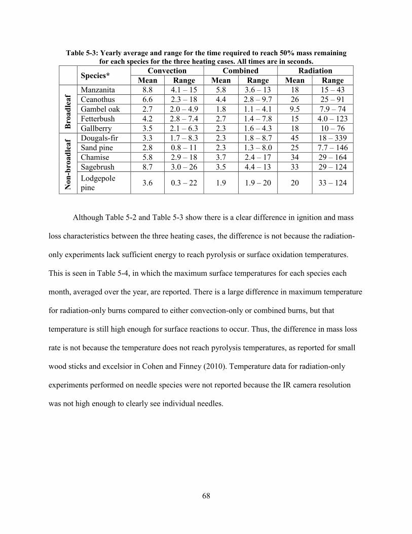
by the root mean squared error (RMSE) for each model. RMC = relative moisture 57 Table 5-1: Flame characteristics derived from video data. 62 Table 5-2. Effect of heating mode on ignition variables. Table entries indicate the 67 Table 5-3: Yearly average and range for the time required to reach 50% mass remaining for
each species for the three heating cases. All times are in seconds. 68 Table 5-4: Maximum surface temperature (°C) for each species averaged over the year. 69 Table 6-1: Ignition time order listed from shortest to longest. Ignition times are averaged as
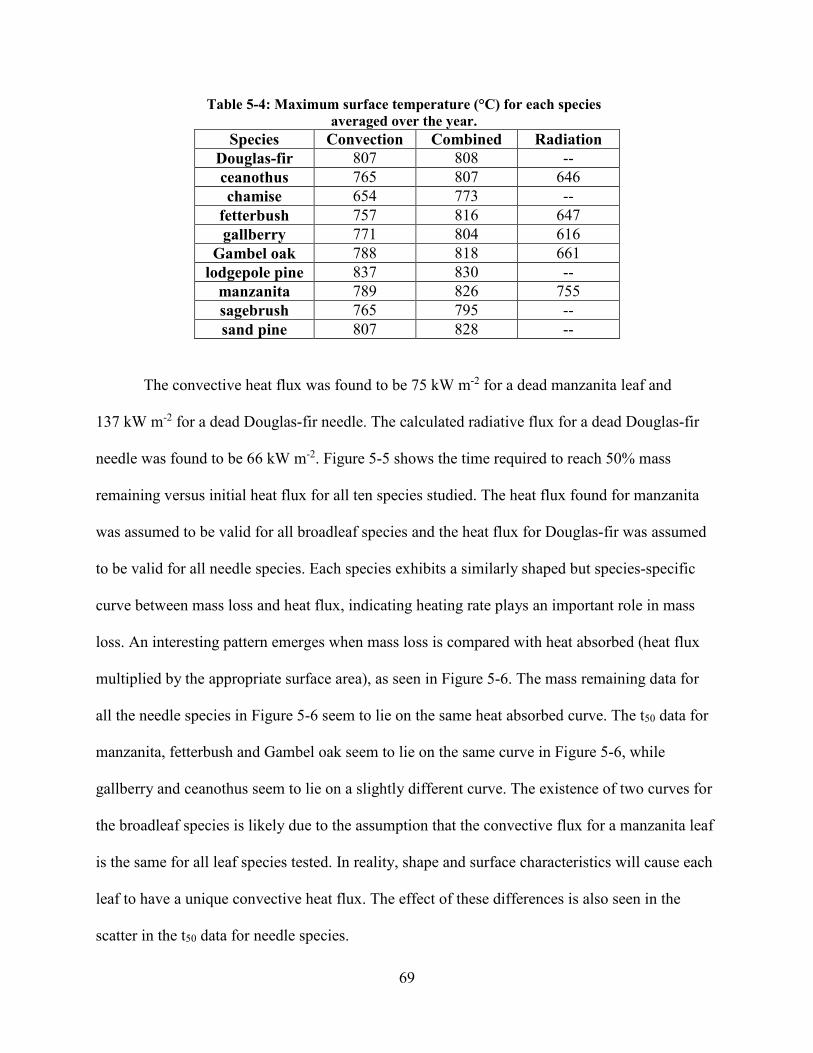
indicated by the column headings. 81 Table 6-2: Order of strongest average correlation to weakest average correlation for needle
species for each of the six listed burning characteristics. MC = moisture content; 83 Table 6-3: Order of strongest average correlation to weakest average correlation for
broadleaf species for each of the six listed burning characteristics. MC = moisture content; 84
Table 6-4. Significance of yearly trends by species. 85 Table 6-5: Adjusted R2 values when regressing flame characteristics for (a) the best overall
model and (b) the model using the most frequent parameters. C means there was no significant model beyond a constant. 86
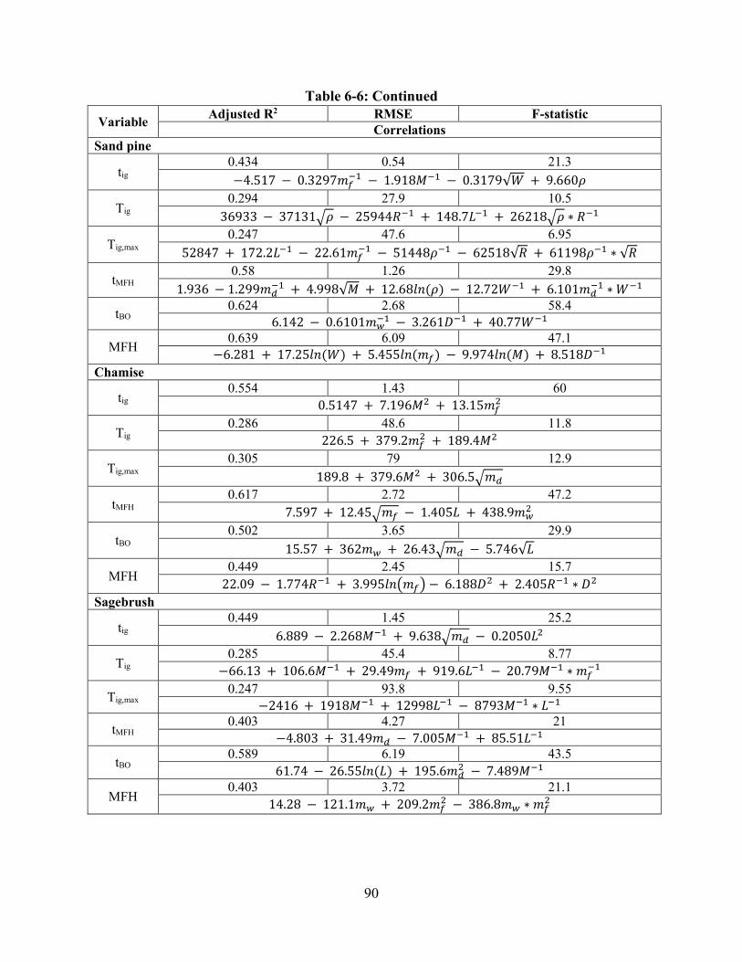
Table 6-6: Best overall correlations for flame characteristics of ten species. 88 Table 6-7: Correlations for flame characteristics for ten species using most frequent
parameters from best-fit correlationss shown in Table 6-6. 92 Table 6-8: Relative uncertainty and sources of measurement error for all the burn
experiment measurements. 99 Table 6-9: Estimated model prediction error due to measurement uncertainty normalized by
the root mean squared error (RMSE) for each 100 Table 6-10: Estimated model prediction error due to measurement uncertainty normalized
by the root mean squared error (RMSE) for 100
ix
Table 7-1: Table of run conditions for all experiments. 104 Table 7-2: Measurement definitions. 105 Table 7-3: Dimensionless numbers relevant to fire behavior near slopes. 118 Table 7-4: Variable definitions for use in dimensionless group calculations and experiment
characterization. 118 Table 7-5: Measured conditions for five documented wildland fires plus the control burns
from the experiments presented in this work. 121 Table 7-6: Conditions for five documented wildland fires estimated from measured data,
plus the control burns from the experiments presented in this work. 121 Table 7-7: Estimates of the dimensionless flame length and heat 122 Table A-1: Experimental data for 16 big sagebrush shrub combustion experiments. 159
x
LIST OF FIGURES
Figure 4-1: Diagram of measurements for broadleaf species. 31 Figure 4-2: Diagram of measurements for needle species, including sagebrush and chamise. 32 Figure 4-3: Apparatus used to measure foliage density. 35 Figure 4-4: Panel showing processing steps for surface area calculations. The left panel is
the normal image, the middle panel is the binary image, and the right panel is the leaf perimeter. 36
Figure 4-5: Ether extractives apparatus showing soxhlet, sampling-containing thimble, condenser, round-bottom flask, solvent, stir bar and heater. 38
Figure 4-6: Flow chart for fuel element property model development 40 Figure 4-7: Yearly patterns for foliage moisture content (MC) and relative moisture content
(RMC) for fetterbush (Fet), gallberry (Gal), sand pine (SP), sagebrush (Sage), lodgepole pine (LP), Gambel oak (Goak), Douglas-fir (DF), chamise, (Cham), manzanita (Manz) and ceanothus (Cean). 42
Figure 4-8: Monthly surface area and width values for gallberry. Error bars indicate the standard deviation in the data. 44
Figure 4-9: Monthly density values for manzanita and Gambel oak. Error bars indicate the standard deviation in the data. 45
Figure 4-10: Monthly thickness values for manzanita, Gambel oak and fetterbush. Error bars indicate the standard deviation in the data. 45
Figure 4-11: Surface area to volume (SA:V) ratio measurements for Gambel oak, fetterbush, gallberry, ceanothus and manzanita. Values shown are in units of inverse centimeters. Error bars indicate the standard deviation in the data. 46
Figure 4-12: Volatiles content, fixed carbon content, ash content and lipid content for manzanita, ceanothus, Douglas-fir, Gambel oak, fetterbush, sand pine and gallberry. Reported values are mass fractions on a dry basis. California species are on the left, Southern in the middle, and Rocky Mountain on the right. 47
Figure 4-13: Dry mass data, probability distribution function (pdf), cumulative distribution function (cdf) and empirical distribution function (edf) for species from the California region (left panel) and Southern region (right panel). 49
Figure 4-14: Dry mass data, probability distribution function (pdf), cumulative distribution function (cdf) and empirical distribution function (edf) for species from the Rocky Mountain region. 50
Figure 4-15: Physical property predictions for manzanita. 54 Figure 4-16: Physical property predictions for Douglas-fir. 55 Figure 5-1: Schematic of flat-flame burner. 61 Figure 5-2: Flame height versus time curve for a single fetterbush run. Points in time
identified by red circles include ignition time, time to maximum flame height, burnout time and maximum flame height. All times were measured relative to the start time (t = 0). 62
xi
Figure 5-3: Example of image processing. The visual image is on the left, the binary image with the flame perimeter identified is on the right. Only contiguous pixels containing flame were categorized as part of the flame. 63
Figure 5-4: Infrared image for a convection-only manzanita run. The leaf is in the middle of the image, glowing red. 63
Figure 5-5: Time required to reach 50% mass remaining versus heat flux for all three heating cases for all ten species. 70
Figure 5-6: Time required to reach 50% mass remaining versus heat absorbed for all three heating cases for all ten species. 70
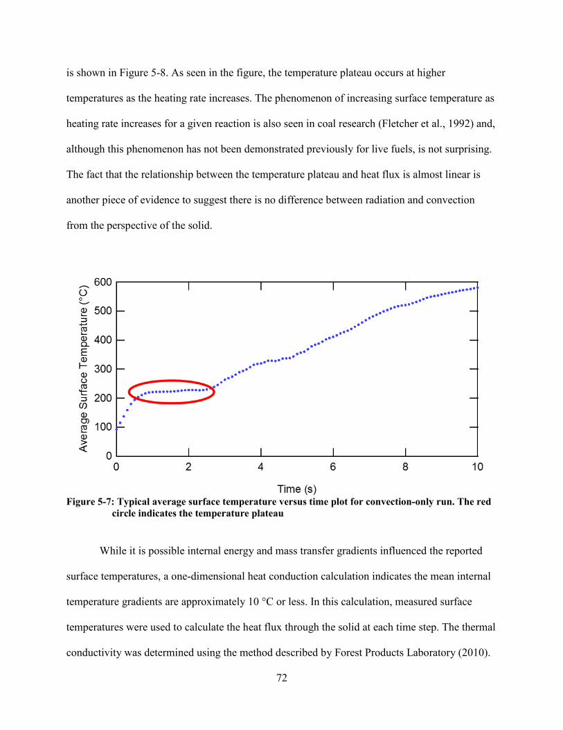
Figure 5-7: Typical average surface temperature versus time plot for convection-only run. The red circle indicates the temperature plateau 72
Figure 5-8: Plateau temperature versus heat flux for five boradleaf species for the three heating cases. 73
Figure 6-1: Results of sample condition experiments for chamise branch segments. The left pane shows the time required to reach 50% mass reamining (t50); the right pane shows the t-test results for the different comparisons. Error bars represent one standard deviation. SDAN=slow drying, all needles; NDAN=no drying, all needles; NDHN=no drying, half needles; QDAN=quick drying, all needles; QDHN=quick drying, half needles. 78
Figure 6-2: Ignition time versus month (left column) and moisture content (right column). Manz = manzanita, Cean = ceanothus, Cham = chamise, Fet = fetterbush, Gal = gallberry, SP = sand pine, DF = Douglas-fir, Goak = Gambel oak, Sage = sagebrush, LP = lodgepole pine. 79
Figure 6-3: Ignition temperature versus month (left column) and moisture content (right column). Manz = manzanita, Cean = ceanothus, Cham = chamise, Fet = fetterbush, Gal = gallberry, SP = sand pine, DF = Douglas-fir, Goak = Gambel oak, Sage = sagebrush, LP =lodgepole pine. 80
Figure 6-4: Parity plots for ignition temperatures for manzanita. Best overall models are shown in the left column, models using the most common predictors are shown in the right column. 95
Figure 6-5: Parity plots for burning characteristics for manzanita. Best overall models are shown in the left column, models using the most common predictors are shown in the right column. 96
Figure 6-6: Parity plots for burning characteristics for Douglas-fir. Best overall models are shown in the left column, models using the most common predictors are shown in the right column. 97
Figure 6-7: Parity plots for ignition temperatures for Douglas-fir. Best overall models are shown in the left column, models using the most common predictors are shown in the right column. 98
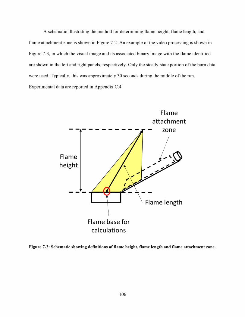
Figure 7-2: Schematic showing definitions of flame height, flame length and flame attachment zone. 106
xii
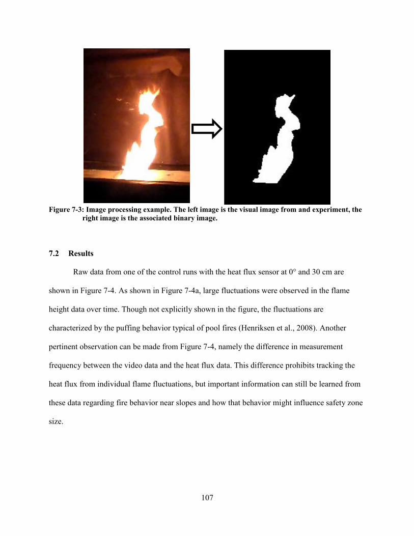
Figure 7-3: Image processing example. The left image is the visual image from and experiment, the right image is the associated binary image. 107
Figure 7-4: Transient flame height data in centimeters (a) and radiative heat flux data in kilowatts per square meter (b) for a control run at 0° and 30 cm. 108
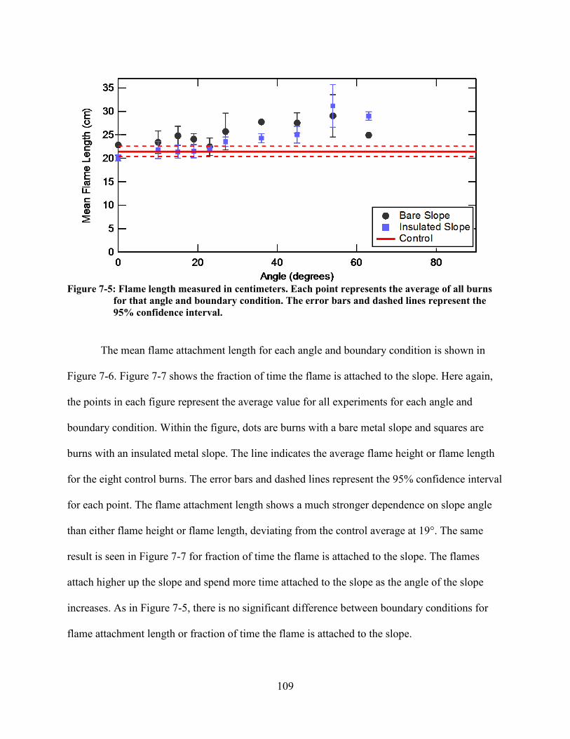
Figure 7-5: Flame length measured in centimeters. Each point represents the average of all burns for that angle and boundary condition. The error bars and dashed lines represent the 95% confidence interval. 109
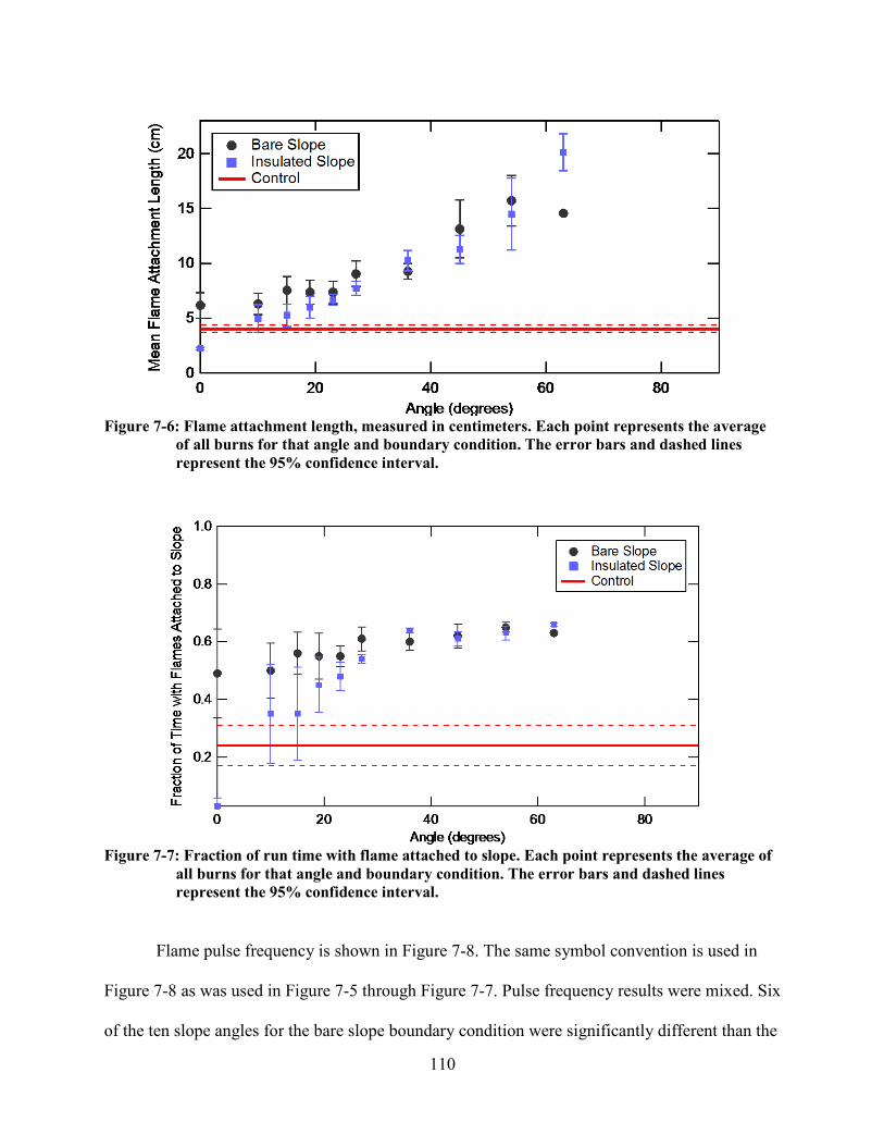
Figure 7-6: Flame attachment length, measured in centimeters. Each point represents the average of all burns for that angle and boundary condition. The error bars and dashed lines represent the 95% confidence interval. 110
Figure 7-7: Fraction of run time with flame attached to slope. Each point represents the average of all burns for that angle and boundary condition. The error bars and dashed lines represent the 95% confidence interval. 110
Figure 7-8: Flame pulse frequency, measured in hertz (Hz). Each point represents the average of all burns for that angle and boundary condition. The error bars and dashed lines represent the 95% confidence interval. 111
Figure 7-9: Average radiative heat flux, measured in kilowatts per square meter (kW m-2). Each point represents the average of all burns for that angle and boundary condition. The error bars and represent the 95% confidence interval. 113
Figure 7-10: Average convective heat flux, measured in kilowatts per square meter (kW m-
2). Each point represents the average of all burns for that angle and boundary condition. The error bars and represent the 95% confidence interval. 113
Figure 7-11: Average convective and radiative heat flux for bare metal and insulated slopes. Each point represents the average of all burns for that angle and boundary condition. The error bars and represent the 95% confidence interval. 114
Figure 7-12: Average and maximum total heat flux for bare metal and insulated slopes. Each point represents the average of all burns for that angle and boundary condition normalized against the mean and maximum values for the 0° control burn. The error bars and represent the 95% confidence interval. 116
Figure 7-13: Angle at which the deviation from control levels becomes significant for each the burn characteristics on the x-axis. Labels on the x-axis are those shown in Table 7-2. Pulse frequency is not shown here because there was no significant deviation from control levels. 117
Figure 7-14: Dimensionless flame attachment length (LAttach) versus slope angle. The solid line is the dimensionless attachment length for the control burns; the dashed line is the dimensionless flame length for the control burns. 119
Figure 7-15: Dimensionless heat flux upslope (FluxAttach) versus slope angle. The solid line is the dimensionless heat flux for the control burns; the dashed line is the heat release rate for the control burns. 120
Figure 7-16: Dimensionless flame attachment length (LAttach) versus slope angle. The solid line is the dimensionless attachment length for the control burns; the dashed line is the dimensionless flame length for the control burns. The triangles represent the estimates of flame attachment from reported data for five documented wildland fires. 123
xiii
Figure 7-17: Dimensionless heat flux upslope (FluxAttach) versus slope angle. The solid line is the dimensionless heat flux for the control burns; the dashed line is the heat release rate for the control burns. The triangles represent the estimates of heat flux from reported data for five documented wildland fires. 123
Figure A-1: Schematic illustration of the wind tunnel at the Pacific Southwest Research Station of Forest service in Riverside, CA (Lozano, 2011) 155
Figure A-2: Comparison of (a) picture of a manzanita shrub and (b) manzanita shrub simulated. 157
Figure A-3: Maximum solid temperature of each area with respect to time for a manzanita shrub combustion experiment with no wind. 161
Figure A-4: Burning big sagebrush stems after the foliage burnout. 161 Figure A-5: Δzf,max comparison of current model (box plots of minimum, first quartile,
median, third quartile and maximum) and wind tunnel experiments (dots) (Prince, 2014) 163
Figure A-6: Burn time comparison of model simulations (box plots of minimum, first quartile, median, third quartile and maximum) and wind tunnel experiments (dots) (Prince, 2014) 163
Figure A-7: Comparison of predicted flame behavior in a manzanita shrub (left) using the semi-empirical shrub combustion model vs. the measured flame behavior in a wind tunnel. 164
Figure B-1: Parity plots for chamise 166 Figure B-2: Parity plots for sagebrush 166 Figure B-3: Parity plots for ceanothus 167 Figure B-4: Parity plots for fetterbush 168 Figure B-5: Parity plots for gallberry 169 Figure B-6: Parity plots for Gambel oak 170 Figure B-7: Parity plots for lodgepole pine 171 Figure B-8: Parity plots for sand pine 172 Figure B-9: Parity plots for ceanothus—best overall models 173 Figure B-10: Parity plots for chamise—best overall models 174 Figure B-11: Parity plots for fetterbush—best overall models 175 Figure B-12: Parity plots for gallberry—best overall models 176 Figure B-13: Parity plots for Gambel oak—best overall models 177 Figure B-14: Parity plots for lodgepole pine—best overall models 178 Figure B-15: Parity plots for sagebrush—best overall models 179 Figure B-16: Parity plots for sand pine—best overall models 180 Figure B-17: Parity plots for ceanothus—models using MCP 181 Figure B-18: Parity plots for chamise—models using MCP 182 Figure B-19: Parity plots for fetterbush—models using MCP 183 Figure B-20: Parity plots for gallberry—models using MCP 184 Figure B-21: Parity plots for Gambel oak—models using MCP 185 Figure B-22: Parity plots for lodgepole pine—models using MCP 186 Figure B-23: Parity plots for sagebrush—models using MCP 187
xiv
Figure B-24: Parity plots for sand pine—models using MCP 188 Figure C-1: Sample temperature plateau curves for all ten species. Broadleaf species are in
the left column, needle species are in the right column. 190
1
1 INTRODUCTION
Knowledge of the role that wildland fire plays in shaping the landscapes in North
America has dramatically increased over the past 60 years. With this knowledge, federal
wildland fire policy in the United States has evolved. The focus a century ago was on fire
suppression. Over the last century, this practice has resulted in an increase in fuel density in the
form of forest litter and small shrubs, causing an escalation in fire intensity and a heightened
awareness that more work is needed to understand the fundamentals of fire spread. Statistics
from the National Interagency Fire Center (National Interagency Fire Center, 2014) support
these conclusions. Data on area burned and suppression costs indicate these numbers have
doubled over the last 20 years, from averages of 2.96 million acres and $371 million between
1985 and 1989 to 5.86 million acres and $1605 million between 2010 and 2014. While the cost
and area burned has increased, the average number of fires has decreased, from 72,000 (1985-
1989) to 65,000 (2010-2014). The trend of larger, more intense fires has not gone unnoticed.
Most work in this area focuses on the causes of these “megafires” and steps to reduce their
frequency (Maditinos and Vassiliadis, 2011; Adams, 2013; Flannigan et al., 2013; Williams,
2013; Liu et al., 2014; Stavros et al., 2014). While not specifically promoting the spread of
megafires, some ecologists have argued that larger fires actually increase the health of forests
and shrublands (Smith et al., 2011; Wan et al., 2014). The current US wildland fire policy
reflects these ideas by holding paramount firefighter safety while recognizing the important
2
ecological functions of fire as well as the economic impact that fire management has on the
budget (Bunsenberg, 2004; Stephens and Ruth, 2005; Fire Executive Council, 2009).
A key component of the current policy is the emphasis on risk management and decision
support systems, which makes it imperative that our understanding of wildland fire be enhanced
and the suite of fire models be improved. Efforts to model wildfires and predict their behavior
have been largely successful for dead, homogenous fuel beds like dry grasslands and forest litter
(Rothermel, 1972; Sullivan, 2009b). Modeling of fire spread in live vegetation is more difficult,
and the lack of knowledge surrounding which physical phenomena drive fire spread in live fuels
increases the uncertainty of the model (Finney et al., 2013). The differences between grasslands,
forests, and shrublands add further difficulty to the problem. Since much of the western United
States is covered by sparsely growing shrubs and small trees (LANDFIRE 1.2.0, 2010), it is vital
to understand those differences so fire managers have more accurate information to guide their
decisions.
Another major emphasis in fire policy is on firefighter safety. During the last 100 years,
thousands of wildland firefighters have been killed or injured in the line of duty (Britton et al.,
2013; Butler, 2014). Of the 900 deaths in that time, 427 were due to firefighter entrapment, the
phenomenon that occurs when the fire passes over the firefighter’s location (Fryer et al., 2013).
While firefighter entrapment fatalities have declined over the last 50 years, they have not been
eliminated (Butler, 2014). Butler (2014) summarized the current challenges in safety zone
determination and listed, among other things, the lack of a theoretical understanding of fires in
live fuels and the lack of understanding regarding the influence of slope angle on fire behavior as
two critical areas where further research is needed. This knowledge will help firefighters better
3
understand where, and how fast, the fire is likely to spread and also help identify locations where
firefighters will be safe if the fire behavior changes drastically.
The National Fire Decision Support Center identified five key areas of fire research that
must be understood in order to improve fire models and thereby improve fire management
strategies and fire fighter safety protocols. This dissertation presents the results of two years of
experimental measurements focusing on two of those key areas, namely the ignition and burning
behavior of live fuels and the differences between convection and radiation in heating live fuels
to ignition. This dissertation also presents work to describe the behavior of fires near slopes and
the influence this behavior has on firefighter safety.
4
2 LITERATURE REVIEW
Ignition of wood and other cellulosic fuels has been studied for over 100 years. Research
has been conducted in many areas that feed into a discussion of wildland fire, including fuel bed
descriptions, requirements for ignition, conditions during burning, predictive modeling
techniques (including rate of spread calculations), and fire fighter safety. The ultimate goal in
wildfire research is two-fold: (1) to understand the physical phenomena that occur within
wildfires, and (2) to develop models that can predict wildfire behavior. Both these research areas
feed into fire fighter safety protocols. Each of the aforementioned research areas will be
discussed briefly: Work to quantify and describe fuel and fuel-bed properties will reviewed in
Section 2.1; research into physical phenomena (requirements for ignition and conditions during
burning) will be reviewed in Section 2.2; modeling techniques will be reviewed in Section 2.3;
the influence of fire behavior near slopes and the resulting effect on firefighter safety zones will
be reviewed in Section 2.4.
Fuel Element Property Measurements and Modeling
Fuel characterization, including physical properties, chemical properties, fuel load, and
fuel location, is an inherent part of any experimental or modeling effort to understand wildland
fire behavior. Characterization of the solid fuel (i.e., grasses, shrubs and trees) can be divided
into three categories: (1) allometric models, (2) three-dimensional (3D) fuel placement models,
and (3) fuel element property models. A discussion of each category follows.
5
Allometric models can predict general fuel properties, such as fuel loading, canopy
height, relative amounts of live and dead fuel, and biomass by size class. These models can be
used in conjunction with remote sensing or ground cover data to describe general fuel properties
over large areas. Considerable work has been done in this area. Most techniques are destructive
and time intensive (Ludwig et al., 1975; Brown, 1976, 1978; Helgerson et al., 1988; Williams,
1989; Schlecht and Affleck, 2014). The main drawback of these models, beyond the labor
necessary to develop them, is their limited applicability—the correlations are specific to both the
fuel type and location. Efforts to improve these models and reduce the required labor through the
use of remote sensing have received increased attention in recent years. Remote sensing data
have been used to measure detailed information about individual plants and general information
about large areas. Seielstad et al. (2011) found that remote sensing can be used to distinguish
foliage and small branches from large branches in Douglas-fir. Skowronski et al. (2007); (2011)
and Barbier et al. (2012) all discuss remote sensing models that predict properties like canopy
bulk density for large areas of land with a high degree of accuracy. A different approach is to use
plant growth theory to predict bulk properties. One such model is that developed by Bartelink
(1998) which allows for growth predictions to be adjusted based on simulated growing
conditions. While these models provide some necessary information to describe solid fuels, they
do not provide all the necessary information. This is seen in the work by Wright (2013), in which
prescribed burn plots with similar fuel loading and fuel type experienced widely different total
burn areas even when accounting for weather variations.
Fuel placement models are those models that seek to capture the natural structure of
plants and the resulting local fuel-density fluctuations. Research has shown fuel bulk density to
be an important variable in fire propagation (Rothermel, 1972; White and Zipperer, 2010;
6
Marino et al., 2012). Work by Parsons et al. (2011) illustrated the need for accurate 3D fuel
characterization. Using a stochastic fuel placement technique called FUEL3D, Parsons et al.
(2011) showed that, for the same mass and volume, fire spread behaves very differently between
fuel beds with homogeneous fuel density and those with variable fuel density. Schwilk (2003)
found that cutting dead fuel from the shrub canopy and placing it on the ground significantly
reduced fire intensity, and thus concluded that canopy structure, not just fuel load, affects fire
behavior. Weise and Wright (2014) cite several other studies which indicate the importance of
fuel arrangement. Prince et al. (2014) developed a fuel placement model for chamise and juniper
based on fractal theory. They used bulk descriptors from Countryman and Philpot (1970) to
provide guidance for the overall shrub properties, then built the shrub using the natural repeating
patterns found in those species. While these models provide the location in 3D space of the
shrub’s trunk, branches and foliage, they do not provide a physical description of the various
shrub parts that affect burning behavior.
Fuel element property models are those models that describe the physical, chemical, and
shape properties of individual leaves or small branch segments. Chemical properties have
received considerable attention (Hough, 1969; Behm et al., 2004), and include properties like
heat capacity, thermal conductivity, and heat of combustion as well as chemical composition
measurements like volatiles content, ash content, structural carbohydrates and ether extractives.
Extensive work has been completed to measure and predict heat capacity and thermal
conductivity for various species of wood (Forest Products Laboratory, 2010) but little has been
done for foliage. Most models for foliage combustion use a form similar to those developed for
wood (Fons, 1946; Engstrom et al., 2004; McAllister et al., 2012; Prince, 2014). Chemical
composition and heat of combustion measurements for foliage are common (Countryman and
7
Philpot, 1970; Rothermel and Philpot, 1973; Countryman, 1982; Frandsen, 1983; Burgan and
Sussot, 1991; Owens et al., 1998; Elder et al., 2011; Jolly et al., 2014). Work has been done to
connect these measurements to flammability and is discussed in Section 2.2.2.
Physical and shape properties have received less attention than chemical properties. Work
by Lyons and Weber (1993) indicated size, shape and orientation of fine fuels could affect
burning behavior. Fons (1946) found that properties like surface area, fuel volume, and foliage
density are important in fire behavior predictions. More recent work (Engstrom et al., 2004;
Fletcher et al., 2007; Shen, 2013) showed fuel orientation and thickness can drastically influence
ignition of shrub foliage. Despite the established effect of these physical properties and
dimensions, there is a startling lack of data in the literature. Countryman and Philpot (1970) and
Countryman (1982) provide excellent descriptions of some common California fuels, including
fuel properties such as ash content, percent extractives, extractive heat content, density, surface
area and volume, but did not report other geometrical properties. Wagtendonk et al. (1996)
measured the diameter, specific gravity and surface-area-to-volume ratio for 19 coniferous
species based on size class and age, but did not report other properties and did not specify if the
needles were used for specific gravity and surface-area-to-volume measurements. Shen and
Fletcher (2015) provided correlations for the geometrical properties of four fuel species to be
used in fire spread models, but did not measure surface area or density, two properties that have
been found to affect fire behavior (Fons, 1946; Lyons and Weber, 1993). Pickett (2008)
measured physical dimensions for several fuels but did not report any prediction models for these
properties, though Prince (2014) reported correlations for manzanita leaves. No other work has
been done to measure or model the physical properties and dimensions of individual fine fuel
8
elements. This lack of data highlights the need to develop these prediction models for other fuel
types so solid fuels can be characterized completely.
Ignition and Burning of Wildland Fuels
Ignition and burning of live forest and shrub fuels are not well understood (Finney et al.,
2013); our understanding must increase if accurate wildland fire prediction models are to be
developed. Current research efforts in this area focus on two questions: (1) Does radiation or
convection dominate in wildland fire spread, and (2) What causes the differences in burning
behavior observed between species and between live and dead fuels. Section 2.2.1 discusses
background work on ignition of wood fuels and foliage. The differences in burning behavior
between live and dead fuels are discussed in Section 2.2.2. The effect of heating mode on
ignition and burning is discussed in Section 2.2.3.
2.2.1 Ignition Time and Temperature
Ignition time and temperature are two empirical phenomena used to describe rate of fire
spread and amount of fuel consumed. Fundamentally, ignition (defined as the onset of a
sustained, visible flame for the purposes of this discussion) occurs when molecules in the solid
break down, enter the gas phase, mix with air and react. Since these phenomena are difficult to
measure, ignition time and temperature are often used as an approximate way to capture these
details. Ignition time is defined as the time elapsed between fuel sample exposure to elevated
temperatures and ignition, and these values are used in modeling to simulate the ignition delay
sequence—pre-heating followed by the onset of pyrolysis. Ignition temperature is defined as the
fuel surface temperature when ignition occurs, and these values are used in modeling to represent
the point at which pyrolysis rates are high enough to support a flame. It should be noted that
9
these two parameters are intimately linked with both the chemical composition and properties of
the individual fuel samples as well as the experimental conditions under which they were
measured. Thus, while these parameters provide a convenient way to discuss results, they do not
convey the complex phenomena occurring during ignition (Smith and King, 1970).
Many studies have been performed during the last century on both wood fuels and foliage
to determine these parameters, with the bulk of the literature focusing on ignition temperature.
Experimental conclusions to date are mixed. Babrauskas (2002, 2003) compiled the results of
ignition temperature experiments on wood fuels and foliage, respectively. After eliminating the
experiments in which the fuel sample was pressed against a hot surface, the reported ignition
temperatures ranged from 200-530°C for wood and 201-450°C for foliage. Babrauskas noted the
large amount of scatter in the data and suggested that, in addition to variations in experimental
setup and measurement techniques, sample condition (e.g. moisture content and size) and species
could affect ignition temperature.
Wildland fire observations that species burn differently support Babrauskas’s postulate
that plant species could be one source of variation in measured ignition temperatures (Fletcher et
al., 2007). However, results by Susott (1982) showed that material ground from various plant
species has the same heat of combustion and similar TGA (thermogravimetric analysis) pyrolysis
mass release curves, and should therefore burn similarly. Thus, one possible explanation for the
observed differences in ignition properties is the shape and structure of the plant and the effect
shape has on heat and mass transfer. However, this explanation has not been tested
experimentally. Most empirical correlations used to predict ignition behavior, particularly for
live fuels, are species specific (Xanthopoulos and Wakimoto, 1993; Dimitrakopoulos and
10
Papaioannou, 2001; Smith, 2005; Pellizzaro et al., 2007; Shen, 2013). Work must be done to
understand the differences in ignition behavior between various species.
2.2.2 Effect of Moisture on Ignition Characteristics and the Differences between Live and Dead Fuels
Investigation of the effect of moisture content on ignition has been studied extensively
and supports Babrauskas’ postulate that sample condition affects ignition. Moisture has been
shown to increase both ignition time (Fons, 1950; Xanthopoulos and Wakimoto, 1993; Gill and
Moore, 1996; Shu et al., 2000; Dimitrakopoulos, 2001) and ignition temperature (Moghtaderi et
al., 1997; Catchpole et al., 2002; Smith, 2005) for various fuels. There are many possible reasons
for this delay. Dilution of pyrolysis gases with non-combustible gases has been cited as a method
for fire suppression (Fons, 1950; Browne, 1958; Catchpole et al., 2002; Lu et al., 2004; Ferguson
et al., 2013). Ferguson et al. (2013) also show that gas-phase temperature is reduced as moisture
increases, which should slow heat transfer to the surface and reduce the surface temperature.
Haseli et al. (2011) and Leroy et al. (2010) have shown pyrolysis to be a strong function of
surface temperature. A slight discrepancy seems to arise at this point in the discussion. Moisture
increases ignition temperature, but also decreases the gas temperature surrounding the solid
which should decrease the solid temperature. One possible explanation for this problem is that
the rate of pyrolysis required to sustain a flame is greater due to dilution by water. Thus, ignition
is delayed until the higher rate of pyrolysis is achieved and a higher average surface temperature
is measured at ignition.
While these results are insightful, most of the previous research on moisture effects has
been performed on dead fuels that have been pre-treated to a specified moisture content.
Xanthopoulos and Wakimoto (1993) performed seasonal experiments on three western conifer
11
species. Fresh cut branch segments (10-15 cm in length) were burned in heated air at
temperatures between 400 °C and 640 °C. Correlations were developed to predict ignition time
based on air temperature and fuel moisture content. Results showed trends are non-linear and
vary with species. Researchers at Brigham Young University (BYU) have collectively performed
thousands of experiments on individual fuel elements in the last decade (Engstrom et al., 2004;
Smith, 2005; Fletcher et al., 2007; Pickett, 2008; Pickett et al., 2009; Pickett et al., 2010; Cole et
al., 2011; Prince, 2014; Prince and Fletcher, 2014; Shen and Fletcher, 2015). Samples, composed
of individual leaves for leaf species and 4 – 6 cm branch segments (<6 mm diameter) for needle
species, were burned in 1000 °C post-flame gases with 10 mol% oxygen to more closely
resemble the conditions of wildland fires (Butler et al., 2004a). Initial experiments were used to
compare live and dead fuels with similar moisture contents, describe qualitatively and
quantitatively the physical changes that occur during live fuel combustion, and determine if
flaming ignition would occur without direct flame contact. Observations regarding the link
between live fuel ignition and moisture were also reported. Work by Fletcher et al. (2007) and
Prince and Fletcher (2013) has shown live fuels release moisture differently than dead fuels.
Water evaporation in dead fuels has been assumed complete in fine fuels once the sample
temperature passes 100°C (Albini, 1967; Rothermel, 1972), but Fletcher et al. (2007) showed
there is still a significant amount of moisture in live fuels when ignition occurs. Pickett (2008)
showed water release still occurring at surface temperatures in excess of 200°C and Prince
(2014) showed significant differences in the temperature profiles of live and dead foliage during
ignition and burning even with the same moisture content. Work by McAllister et al. (2012)
showed significant differences in the ignition behavior between live and dead pine needles.
Additionally, work by Weise et al. (2005a) demonstrated live fuels can burn with moisture levels
12
in excess of 100% on a dry-weight basis while dead fuels are rarely able to sustain combustion
when moisture content is above 30-35% (Hawley, 1926; Lindenmuth and Davis, 1973). Tiaz and
Zeiger (2010) indicate plant response to environmental stresses like drought causes accumulation
of non-structural carbohydrates within plant cells that could affect flammability. These
differences have led researchers to postulate that there is significant interaction between the free
water and the cells in live plants that does not occur in dead plants (McAllister et al., 2012;
Prince and Fletcher, 2013). Finney et al. (2013) postulated that water release in live fuels is not
complete until breakdown of the cellular structure occurs. Still other work has been done
indicating root structure (Pellizzaro et al., 2007), plant dry mass (Jolly et al., 2014), chemical
composition (Pyne et al., 1996; McAllister et al., 2012), tree sex (Owens et al., 1998) and post-
fire regeneration strategy (Cowan, 2010) could have a larger effect on ignition of live fuels than
moisture content, though results are mixed in work to quantify the effect of chemical
composition (Alessio et al., 2008). Several studies have been published indicating flammability
changes with season but not necessarily with moisture content (Philpot, 1969; Wright and
Bailey, 1982; White, 1994; Rodriguez Anon et al., 1995; Bianchi and Defosse, 2015). White and
Zipperer (2010) review work done on the flammability of live foliage and conclude moisture
content has the largest effect on ignition (Etlinger and Beall, 2004; Weise et al., 2005b; Alessio
et al., 2008). There are some dissenting opinions (Alexander and Cruz, 2013), but the general
consensus is that live fuels burn differently than dead fuels and that moisture has a significant
effect on burning characteristics for both live and dead fuels. In summary, a fundamental
understanding of the physical processes that drive live fuel combustion is both absent and
necessary if predictive models are to be developed.
13
Another difficulty in evaluating the effects of moisture levels on foliage combustion is
the presence of light hydrocarbons (ether extractives such as fats, waxes and terpenoids) in live
foliage (Philpot and Mutch, 1970; Susott, 1980). While structural carbohydrate (cellulose,
hemicellulose, and lignin) content within foliage changes very little once a leaf is fully
developed, levels of non-structural carbohydrates, extractives and water experience fluctuations
in response to season and climatological conditions (Kozlowsk and Clausen, 1965; Little, 1970;
Gilmore, 1977; Kainulainen et al., 1992; Jolly et al., 2014). These extractives have the highest
heat content of any forest fuel (Nunez-Regueira et al., 2005) and often decompose and vaporize
at temperatures much lower than accepted ignition temperatures. For example, Mardini et al.
(1989) suggested decomposition temperatures of extractives as low as 50 °C. This early
devolatilization could lead to an increase in flammability for live fuels, and the presence of these
extractives is sometimes cited as the reason for the ability of live fuels to burn under conditions
in which dead fuels do not burn (Finney et al., 2013). These phenomena must be understood if a
fundamental understanding of wildfire spread is to be developed.
2.2.3 Effect of Heat Transfer Mode on Ignition
Many experimentalists and modelers have concluded that radiation heat transfer
dominates in large fires (Simms, 1960; Balbi et al., 2007; Silvani and Morandini, 2009; Paudel,
2013) and fires with little to no wind in homogeneous fuel beds (Morandini et al., 2001; Morvan
and Dupuy, 2001; Sullivan et al., 2003; Morvan and Dupuy, 2004), but the relative effect of
radiation and convection for fires outside these conditions is still unknown (Morandini et al.,
2001; Sullivan et al., 2003). Much of the experimental work looking at heat transfer mode has
focused on dead and woody fuels (Simms, 1960, 1963; McCarter and Broido, 1965; Simms and
Law, 1967; Pagni, 1975; Moghtaderi et al., 1997; Morandini et al., 2001; Dupuy et al., 2003;
14
Gratkowski et al., 2006; Pitts, 2007; Reszka and Torero, 2008; Silvani and Morandini, 2009),
with only a limited amount of work performed for live fuels and foliage (Stocks et al., 2004;
McAllister et al., 2012). Experiments performed by Rothermel (1972) showed fuel pre-heating in
no-wind and backing-fire situations, illustrating radiative heating and leading researchers to
conclude that radiation is the dominant form of heat transfer for fire spread. However, other
experiments have shown that, while pre-heating does occur due to radiation, the bulk of the
temperature rise occurs within a few centimeters of the flame front in no-wind situations (Fang
and Steward, 1969; Baines, 1990) and that significant amounts of pyrolyzates are not formed at
the fuel temperatures associated with radiant pre-heating (Cohen and Finney, 2010). Anderson
(1969) concluded that radiant heat flux can provide no more than 40% of the energy required for
sustained fire spread. Engstrom et al. (2004) showed experimentally that flaming ignition can
occur with convective heating without direct flame contact. Work in the past three years has
shown that convection contributes significantly to intermittent fuel pre-heating and downward
fire spread (Finney et al., 2015). Still other work has shown flame propagation to depend
strongly on direct flame contact with un-burned fuel (Vogel and Williams, 1970; Carrier et al.,
1991). Current operational fire spread models do not differentiate between heat transfer
mechanisms (Sullivan, 2009b, c). This lack of consensus illustrates that a detailed understanding
of heat transfer in fire spread and the mode driving that spread under various conditions is still
missing (Finney et al., 2013).
One reason it is difficult to reach a consensus on heat transfer effects in wildland fire is
that it is problematic to compare results from different data sets due to varying experimental
conditions. For example, McAllister et al. (2012) report ignition characteristics of live fuels
under radiant heating using the FIST apparatus. The experimental setup includes laminar air
15
flowing past the irradiated sample sitting on an insulated balance with an igniter downstream of
the sample. The samples were covered in graphite powder to increase sample emissivity in the
mid-IR wavelength range. Cohen and Finney (2010) exposed fuel samples to similar radiant heat
fluxes as McAllister et al. (2012), but their samples were suspended in air next to the heat source
and they did not use an igniter. The results from both papers are interesting and present useful
information, but it is difficult to compare results between papers due to different experimental
conditions. This is true for convection experiments as well, as seen when comparing the work
published by Xanthopoulos and Wakimoto (1993) and Prince and Fletcher (2014). One question
that has never been explored is whether or not the fuel sample responds similarly to radiation or
convection under the same experimental conditions. The answer to this question can help
facilitate comparison of experimental results between researchers worldwide.
Work to quantify the contributions of radiation and convection in live-shrub combustion
is necessary to understand the basic theory of fire spread and to develop a model that accounts
for both mechanisms of heat transfer. Additionally, exploration of radiant and convective heating
of solid fuel samples under similar experimental conditions can help facilitate comparison of
experimental results. The aim of this project is to explore the effect of heating mode on ignition
and burning behavior to better understand what physical processes drive fire spread in live shrub
and conifer fuels.
2.2.4 Ignition Summary
Ignition occurs when a fuel sample is heated to the point where pyrolysis rates are high
enough to support a gaseous flame and a flammable mixture exists in the gas phase. Researchers
and other fire professionals often simplify this problem by measuring an ignition time and
temperature. These values are then used as empirical estimates of the time it takes to heat the
16
sample and the surface temperature when pyrolysis rates can support a continuous flame,
respectively. While these approximations can capture general trends, they cannot explain the
complex behavior observed in wildland fires. Additionally, ignition time and temperature values
hold little physical meaning because they are dependent on experimental conditions (Finney et
al., 2013). Moisture is known to cause an ignition delay, but the exact mechanisms at work are
still a mystery. Moisture is assumed to be almost completely evaporated before ignition occurs in
fine dead fuels, but a significant amount of moisture is still present at ignition in live fuels
(Fletcher et al., 2007) and in larger dead woody fuels (Williams, 1953; Simms and Law, 1967).
The relative importance of the different heat transfer mechanisms in live-shrub fires is
not well understood. Most early models assume radiation as the dominant heat transfer
mechanism, but experiments have indicated convection (Baines, 1990; Weber, 1991) or direct
flame contact (Fang and Steward, 1969; Vogel and Williams, 1970; Carrier et al., 1991) are also
important in fire spread. A better understanding of these phenomena must be established if
improved predictive models are to be developed.
Wildland Fire Modeling
Wildfire models were summarized and categorized in 1991 as statistical, empirical and
physical (Weber, 1991; Clark, 2008). In a review published in 2009, Andrew Sullivan suggested
a fourth category be added that includes fire spread simulators and differentiated between
physics only and physics and chemistry models (Sullivan, 2009c, b, a). For the purposes of this
review, models will be categorized as statistical models, physical models, empirical models, and
simulation models. Each has its own strengths and weaknesses, and each must be understood in
order to follow current efforts in model development.
17
2.3.1 Statistical Models
Statistical models are based on test fires and contain no explicit physical information.
These models often take two forms—those developed for a specific fuel at specific conditions
and those developed for several species over a broad range of conditions. The first kind are often
very accurate for the conditions and fuels specified, but provide little information outside those
conditions. The second kind provide ballpark information for a large number of fires, but aren’t
accurate enough to provide detailed information (Lindenmuth and Davis, 1973; Weber, 1991).
The Canadian FBPS and Anderson et al. (2015) models are examples of statistical models
(Wotton et al., 2009).
2.3.2 Physical Models
Physical models are based largely in fundamental physics and chemistry principles
(Sullivan, 2009a). Two basic approaches have been used in developing these models. The first
approach is to solve the governing equations in 3D space while the second uses correlations to
approximate the solutions to the governing equations.
As mentioned, models following the first approach seek to solve the basic transport
equations. They also differentiate between different modes of heat transfer and give insight into
fundamental interactions within the flaming zone (Clark, 2008). Current models on this scale are
FIRETEC (Linn, 1997; Linn et al., 2005; Linn and Cunningham, 2005), FDS and its extension
WFDS (McGrattan and Forney, 2005; Mell et al., 2005; Mell et al., 2007) and WRF-
Fire/CAWFE (Coen et al., 2013; Coen and Riggan, 2014; Weise and Wright, 2014). Simulations
using these models can be separated into two categories based on their grid and domain size. The
small-scale simulations use grid cells 1 centimeter in size and cover a domain up to a bush or tree
18
(approximately 1-10 meters). These simulations provide useful insights into fundamental
interactions on leaf-scale (so far as the information is included in the models) but lack the
complex characteristics of large-scale fires and the fire/wind/atmosphere interactions (Clark,
2008). The large-scale simulations use grid cells on the meter scale and cover domains on the
hundred meter (or “hill-side”) scale. These simulations include the complex, large-scale
dynamics that small-scale physical models lack, but are computationally expensive and do not
include small-scale chemical and physical interactions. Clark et al. (2010) generated a sub-grid
thermodynamic equilibrium combustion model based on the mixture fraction to interface with
FIRETEC, with the hope that greater detail could be added to the combustion chemistry without
increasing computational time. While this effort was largely successful, Clark et al. (2010)
highlight the lack of wildfire data available to successfully validate theirs or any such model.
These models can provide useful insights into physical phenomena, but use of these models
assumes the authors knew enough about the physical phenomena to model them correctly.
Additionally, high computational costs make these models ineffective except in prescribed burns,
for post-fire analysis, or for academic purposes (Sullivan, 2009a).
The second approach, used by Albini and Brown (1996); (Balbi et al., 1999); Butler et al.
(2004b); Balbi et al. (2007), and Balbi et al. (2009) is similar in concept to empirical models, but
these models use enough physical detail to be classified as physical models. These models
generally include detail about different modes of heat transfer (Albini, 1985, 1986; Butler et al.,
2004b; Balbi et al., 2007) or chemical kinetics (Balbi et al., 1999) but do not solve the governing
equations. Considerable effort is being put into development of these models with the hope of
producing a model that is computationally fast but generally applicable. This effort has been met
with varying amounts of success, but a widely applicable model has not yet been produced.
19
2.3.3 Empirical Models
Empirical models are compilations of lab-scale experiments into correlations that seek to
account for variables such as wind, slope, fuel type, and moisture content in predicting the rate of
fire spread (Weber, 1991; Clark, 2008). These models are essentially point-source models, where
energy released by one fuel element is transferred to a neighboring fuel element, thereby
initiating the combustion sequence for that fuel element (Fons, 1946; Rothermel, 1972; Albini,
1985; Catchpole et al., 1998; Pickett, 2008). Fons (1946) was the first to attempt a mathematical
model for fire spread. His model treats fire spread as successive ignitions, with particle ignition
time and distance between particles as the two governing parameters. This is the simplest
empirical model and contains many shortcomings. Rothermel (1972) used the same premise as
Fons in defining how fire spread occurs but included much more detail when he developed a
model based on the data from Frandsen (1971). Rothermel introduced a heat of ignition
parameter that defines how much energy must be absorbed by a particle to raise the surface
temperature to its measured ignition temperature, assuming water vaporization occurs at 100 °C.
Rothermel’s formulation forms the basis for most fire spread models developed in the last forty
years. Examples of these models used in the United States include BEHAVE (Rothermel, 1972),
and apparent density were measured at the BYU Wildfire Lab in Provo, UT each month over a
one-year period for ten live fuels (see Table 4-2). On average, 25 replicates were completed each
month. All measurements were made within 48 hours of sample collection—non-local species
were sealed in plastic bags and shipped overnight to Provo. The plastic bags were kept sealed
1 This chapter is under review for publication in Forest Science
31
and out of direct sunlight until measurements could be made. The ten species were categorized as
broadleaf species or needle species based on the shape of the foliage (see Table 4-2). Broadleaf
samples consisted of whole, undamaged leaves while needle samples consisted of 2-6 cm branch
tips with the foliage attached. Sagebrush was categorized as a needle species because the fuel
element used in this work was a section of branch with the foliage attached, even though
sagebrush foliage is comprised of small leaves and not needles. A branch segment was used
because previous work on sagebrush showed that individual leaves did not burn well (Shen,
2013). Foliage samples were also categorized as new (current year) growth or old (previous year)
growth.
Figure 4-1: Diagram of measurements for broadleaf species.
32
Figure 4-2: Diagram of measurements for needle species, including sagebrush and chamise.
Table 4-1: Measurement definitions
Property Broadleaf species Needle species Chamise and sagebrush
Length Distance from leaf base to leaf tip (cm). Length of stem (cm). Length of stem (cm).
Width Largest distance in
direction perpendicular to length (cm).
Largest distance between needle tips
normal to length (cm). N/A
Thickness Measured using calipers
without crossing the main vein (mm).
N/A N/A
Needle length N/A Average needle length on the sample (cm). N/A
Stem diameter N/A Diameter of stem (mm). Diameter of stem (mm).
Mass Mass of sample (g). Mass of sample (g). Mass of sample (g).
33
Table 4-2: Species tested.
Species Region Sampling Location Type Year
chamise (Adenostoma fasciculatum) California Riverside, CA Needle 1 manzanita (Arctostaphylos glandulosa)
California Riverside, CA Broadleaf 2
ceanothus (Ceanothus crassifolius) California Riverside, CA Broadleaf 2 Douglas-fir (Pseudotsuga menziesii var. glauca)
Rocky Mountain Missoula, MT Needle 2
big sagebrush (Artemisia tridentata) Rocky Mountain Provo, UT Needle 1 lodgepole pine (Pinus contorta) Rocky Mountain Missoula, MT Needle 1 gambel oak (Quercus gambelii) Rocky Mountain Provo, UT Broadleaf 2 gallberry (Ilex glabra) Southern Crestview, FL Broadleaf 2 fetterbush (Lyonia lucida) Southern Crestview, FL Broadleaf 2 sand pine (Pinus clausa) Southern Crestview, FL Needle 2 Scientific names cited from USDA, NRCS. 2015. The PLANTS Database (http://plants.usda.gov, 31 March 2015). National Plant Data Team, Greensboro, NC 27401-4901 USA. Year 1 = April 2012-March 2013, Year 2 = April 2013-March 2014.
Physical dimensions include mass, length, width and thickness for broadleaf species and
mass, length, width, needle length and stem diameter for needle species. See Table 4-1 for
definitions. Moisture content (MC) was measured on a dry basis (see Equation 4-1) using a
Comptrac Max1000 analyzer2 with a drying temperature of 95°C and a minimum sample size of
1 gram. Relative moisture content (RMC) was measured on a turgid basis (see Equation 4-2);
turgid mass (mass of sample when fully saturated with water) was determined by soaking the
sample in water for 24 to 48 hours before weighing. The minimum sample size for RMC was
also 1 gram. Because several leaves or branch sections were necessary to reach the required
minimum weight, the reported MC and RMC were an average of the fuel elements used in the
measurements.
2 The use of trade or firm names in this publication is for reader information and does not imply endorsement by the U.S. Department of Agriculture of any product or service.
Significant monthly trends were found for density (manzanita and Gambel oak), surface
area (gallberry), thickness (manzanita, Gambel oak and fetterbush) and width (gallberry), as
shown in Figure 4-8 through Figure 4-10. Surface area and width for gallberry both followed a
similar trend (see Figure 4-8); large leaves were observed in April, small leaves in July and
44
relatively large leaves from August to the next April. Density for manzanita was high in April,
decreased rapidly to a low in August, and then increased slowly through March (see Figure 4-9).
Density for Gambel oak showed the opposite trend, with lows in May and October and a high in
August. Thickness for manzanita, Gambel oak and fetterbush all showed the same pattern: high
in the spring, low in the summer, then increasing slowly through the rest of the sample period
(see Figure 4-10). Changes in density and thickness for manzanita compared to Gambel oak
show some interesting relationships. Thickness and density for manzanita seemed to be
correlated fairly well with each other (R2 = 0.76), but the observed seasonal changes did not
correlate solely to changes in MC (R2density = 0.25, R2
thickness = 0.12). The trends for Gambel oak
thickness and density were not well correlated (R2 = 0.10). The trend for Gambel oak thickness is
at least partly due to MC (R2 = 0.40) while that for density had no relationship to MC (R2 =
0.00). The R2 values presented here represent the amount of variation in the response variable
that is accounted for by the associated linear regression model.
Figure 4-8: Monthly surface area and width values for gallberry. Error bars indicate the standard
deviation in the data.
45
Figure 4-9: Monthly density values for manzanita and Gambel oak. Error bars indicate the
standard deviation in the data.
Figure 4-10: Monthly thickness values for manzanita, Gambel oak and fetterbush. Error bars
indicate the standard deviation in the data.
Surface area to volume (SA:V) ratio measurements are shown in Figure 4-11 for all five
broadleaf species. The SA:V ratio varies during the spring and summer but levels off during the
fall and winter months. Species from the same location have nearly identical trends. Gambel oak
46
consistently exhibited the largest SA:V ratio with the exception of May, when the leaves were
still forming. Fetterbush and gallberry had similar SA:V ratios to that for Gambel oak during the
spring and early summer, but those values dropped during fall and winter. Manzanita and
ceanothus had consistently lower SA:V ratios than the other broadleaf species.
Figure 4-11: Surface area to volume (SA:V) ratio measurements for Gambel oak, fetterbush,
gallberry, ceanothus and manzanita. Values shown are in units of inverse centimeters. Error bars indicate the standard deviation in the data.
4.2.2 Chemical Composition Measurements
Data for volatiles content, fixed carbon content, ash content and lipid content are reported
as mass fractions on a dry basis and are shown in Figure 4-12. Aside from Gambel oak, which
shows an 8% change in volatiles and fixed carbon content, chemical composition measurements
were constant throughout the year. The yearly mean for each measurement is shown in Table
4-5. The chemical composition measurements reported here show minimal differences between
species. Susott et al. (1975) and Susott (1982) showed 17 different foliage samples all had
47
California Southern Rocky Mountain
Figure 4-12: Volatiles content, fixed carbon content, ash content and lipid content for manzanita, ceanothus, Douglas-fir, Gambel oak, fetterbush, sand pine and gallberry. Reported values are mass fractions on a dry basis. California species are on the left, Southern in the middle, and Rocky Mountain on the right.
48
similar heats of combustion and mass release curves. The result that the ten species studied
herein all have similar volatiles contents agrees with results by Susott (Susott et al., 1975; Susott,
1982), and provides evidence that foliage samples are chemically similar. The result that
different species are chemically similar has important implications for fire modeling. Many
physics-based models simplify surface chemistry through the use of one-step and two-step
devolatilization models and by assuming generic properties for the solid fuel (Morvan and
Dupuy, 2001; Mell et al., 2007). While these simplified models were shown to be inadequate for
predicting mass loss in live manzanita leaves (Prince, 2014), it is possible that more sophisticated
surface chemistry models would also predict similar mass loss behavior between species. These
results are at odds with reported differences in burning behavior between species (Fletcher et al.,
2007); future work must be done to understand these differences.
Table 4-5: Yearly average values of volatiles content, fixed carbon content, ash content and lipid content for manzanita, ceanothus, Douglas-fir, Gambel oak, fetterbush,
sand pine and gallberry.* Species Volatiles Content Fixed Carbon Content Ash Content Lipid Content
Gambel oak 0.812 0.159 0.029 0.058 * All values are reported on a dry basis
4.2.3 Dry Mass Distribution
The estimated parameter values, the 95% confidence intervals on the means and the p-
value from the Kolmogorov-Smirnov test are shown in Table 4-6. All the species except
ceanothus are statistically verified as Weibull distributions at the 95% confidence level while
ceanothus is verified at the 90% confidence level. There were no distinct seasonal trends in the
49
mass data (see Table 4-3 and Table 4-4), so the distribution is valid for the entire year. Plots
containing the collected data, probability density function (pdf), empirical cumulative
distribution function (edf) and theoretical cumulative distribution function (cdf) are shown in
Figure 4-13 (left panel) for California species, Figure 4-13 (right panel) for Southern species and
Figure 4-14 for Rocky Mountain species.
California Southern
Figure 4-13: Dry mass data, probability distribution function (pdf), cumulative distribution function (cdf) and empirical distribution function (edf) for species from the California region (left panel) and Southern region (right panel).
50
Table 4-6: Weibull distribution parameters for measured dry mass calculated using Equations 4-5 and 4-6.
Figure 4-14: Dry mass data, probability distribution function (pdf), cumulative distribution function (cdf) and empirical distribution function (edf) for species from the Rocky Mountain region.
4.2.4 Prediction Models
The prediction models for the various fuel element characteristics are shown in Table 4-7
(Broadleaf) and Table 4-8 (Needle). The models are reported in the order in which they were
developed and are intended to be used. The strength of these models is shown by the amount of
51
data variation accounted for by the model. For the overall collection of models, 36% have an R2
values greater than 0.7 and 72% have an R2 value greater than 0.5. When broken out by species
type, 50% of the broad leaf species models have and R2 value greater than 0.7 and 90% of the
models greater than 0.5. The needle species were less successful, with 17% and 48% of the
models having an R2 value greater than 0.7 and 0.5, respectively. The difference between needle
and broadleaf species models likely could have been overcome if the number of needles per
sample was measured for the needle species.
None of the models developed here contain a seasonal parameter. While this lack of a
seasonal parameter is not typical for plant growth models or models predicting plant
characteristics (Adams, 2014), the constancy of the measured data throughout the year made the
inclusion of a seasonal parameter unnecessary. The measured characteristics that did change with
season were accompanied by changes in other characteristics (usually moisture content) so that
the single prediction model is valid for the whole year. Some of the needle species, particularly
sand pine, did exhibit some visual seasonal variation in the shape and size of individual fuel
samples that was not captured by the statistical test for seasonal trends. However, there is enough
scatter in the data for sand pine that the differences based on growing season are
indistinguishable from the general trends reported here. Parity plots for all the manzanita and
Douglas-fir models are shown in Figure 4-15 and Figure 4-16, respectively. Model parity plots
for the other eight species are shown in Appendix B.1.
52
Table 4-7: Fuel element property models for broadleaf species. Parameter R2Adj Model Ceanothus
Figure 4-15: Physical property predictions for manzanita.
4.2.5 Uncertainty Analysis
As with any experimental work, it is important to explore the effect of measurement error
on both the measured values themselves and on the models which use the data. Table 4-9 details
both the sources of error and the relative magnitude of those errors for each pre-burn
measurement. Within the table, the relative uncertainty entries represent the measurement
uncertainty normalized by the measured value averaged across all species and months. The
55
maximum relative uncertainty is 33% for the ash content measurements, and is largely due to the
small amount of ash contained in the samples. Other than ash, all the other relative uncertainties
are below 5%, indicating the natural scatter in the data is far more important than measurement
uncertainty in developing prediction models.
Figure 4-16: Physical property predictions for Douglas-fir.
56
Table 4-9: Relative uncertainty and sources of measurement error for all the pre-burn measurements.
Measurement Relative Uncertainty Sources of Error
Moisture content 0.0001 Computrac runs drying program and reports moisture content. Error is that reported by manufacturer
Relative moisture content
0.0017 Error source is the sensitivity of the mass balance
Density 0.0053 Error source is the sensitivity of the mass balance Length 0.014 Error comes from the tick mark spacing on the ruler Width 0.015 Error comes from the tick mark spacing on the ruler Needle length 0.011 Error comes from the tick mark spacing on the ruler Thickness 0.025 Error comes from the specification on the caliper Stem diameter 0.006 Error comes from the specification on the caliper
Surface area 0.017 Error comes from user input on the algorithm’s reference
length scale and from the error on the thickness measurement
Fresh mass 0.0005 Error source is the sensitivity of the mass balance Dry mass 0.001 Error source is the sensitivity of the mass balance Water mass 0.001 Error source is the sensitivity of the mass balance Lipid content 0.04 Error source is the sensitivity of the mass balance Volatiles content 0.0012 Error source is the sensitivity of the mass balance Fixed carbon content
0.013 Error source is the sensitivity of the mass balance
Ash content 0.33 Error source is the sensitivity of the mass balance
The entries in Table 4-10 represent the estimate of the model error due to measurement
uncertainty, using analytical propagation of error techniques, divided by the root mean squared
error (RMSE) of the residuals between the data and the prediction. Thus, a table entry greater
than one (highlighted in the table) indicates that the estimated effect of measurement uncertainty
is greater than the average model residual. The entries listed in Table 4-10 for Gambel oak
relative moisture content and density are high because the model agreement with the data is very
good, with R2 values near 1, and hence the RMSE value is close to zero. Only the entries in the
Table 4-10 for sagebrush (RMC and length) and lodgepole pine (diameter) are greater than one
and have relatively high RMSE values. The average for the entries with values less than one is
0.11. The results in Table 4-10 indicate the same conclusion drawn from Table 4-9, namely, that
57
the measurement uncertainty does not have a large effect on the prediction models show in Table
4-7 and Table 4-8.
Table 4-10: Estimated model prediction error due to measurement uncertainty normalized by the root mean squared error (RMSE) for each model. RMC = relative moisture
thickness, stem diameter, needle length, surface area, surface area to volume ratio, mass,
volatiles content, fixed carbon content, ash content and lipid content. An alternate method for
measuring foliage apparent density using oil instead of water was developed and used. Whole-
leaf surface area measurements are reported that do not require approximating the sample with
an idealized shape. Foliage dry mass distributions were developed that allow the user to calculate
the dry mass for a single leaf or branch tip. Prediction models were developed for each measured
property based on sample dry mass and moisture content. Most measured sample characteristics
did not change throughout the year, making the use of a seasonal parameter in model
development unnecessary. Sample characteristics that did change throughout the year were
associated with changes in the other characteristics (usually moisture content) so that the models
developed here are accurate for the entire year. It is anticipated that these models can be used in
59
conjunction with bulk fuel description models and fuel placement models to describe the fuel
matrix in detail for comprehensive fire spread models.
60
5 THE EFFECT OF HEATING MODE ON IGNITION AND BURNING OF TEN LIVE FUEL SPECIES3
Methods
5.1.1 Experiment Description
Combustion experiments (25 replicates for each species) were performed each month in
the flat flame burner (FFB) apparatus at Brigham Young University (BYU) (see Figure 5-1). In
total, ten species were tested over a two-year period. Experiments were performed each month
using three heating cases: convection only, radiation only, and both convection and radiation
combined. Pre-burn measurements, including moisture content, relative moisture content, mass,
density, length, width, needle length, stem diameter, thickness and surface area, are described in
Section 4.1.1. Video images, mass and temperature data were collected using the apparatus
shown in Figure 5-1. Samples were individually weighed and placed within the apparatus. The
water-cooled FFB produced exhaust gases at 1000°C and 10 mol% oxygen that flowed past the
sample suspended on a holding rod using an alligator clip. The holding rod was connected to a
Mettler Toledo XS204 Cantilever mass balance. Mass data were continuously measured using
National Instruments Labview 8.6 software. A glass cage surrounding the sample prevented
ambient air from being entrained in the FFB exhaust gases. An Omega K-type thermocouple
(0.013 mm diameter, 0.05 s response time) was used to measure the gas temperature. Smith
3 This chapter is under review for publication in Combustion Science and Technology
61
(2005) corrected these temperature measurements for thermocouple radiation losses and found
the losses to be small at these temperatures. An Omega QH-101060 radiant panel was used to
provide a 50 kW m-2 flux at the sample location; radiant heat flux was measured using a
Medtherm 64-series heat flux sensor.
Figure 5-1: Schematic of flat-flame burner.
Flame videos were captured using a Panasonic SDR S50 Camcorder; surface temperature
videos were collected using a FLIR A20M infrared camera. Visual and infrared video data were
post-processed to extract the burn characteristics listed in Table 5-1. Flame characteristics listed
in Table 5-1 are illustrated in Figure 5-2. A visual image and its associated binary image are
shown in Figure 5-3 to demonstrate image processing techniques. Figure 5-4 contains an infrared
image with its associated temperature scale. A few experiments with radiant fluxes of 60 kW m-2
62
and 35 kW m-2 were performed using Gambel oak to further explore the effects of heating mode
versus heat flux.
Table 5-1: Flame characteristics derived from video data. Variable Description Ignition Time (tig) Time when a visible, sustained flame appears (s). Burnout Time (tbo) Time when the flame disappears (s). Maximum Flame Height (MFH) Height of tallest flame during a run (cm). Time to Max Flame Height (tmfh) Time when tallest flame occurs (s). Surface Temperature (Tig) Average surface temperature at time of ignition (°C). Maximum Ignition Temperature (Tig,max)
Maximum surface temperature at the time of ignition (°C).
Fraction Remaining at Ignition (Xig) Mass at ignition divided by initial mass (fraction). Mass Loss Rate at Ignition (��𝑚𝑑𝑑𝑖𝑖) Instantaneous mass loss rate at ignition divided by initial
mass (% s-1).
Figure 5-2: Flame height versus time curve for a single fetterbush run. Points in time identified by
red circles include ignition time, time to maximum flame height, burnout time and maximum flame height. All times were measured relative to the start time (t = 0).
63
Figure 5-3: Example of image processing. The visual image is on the left, the binary image with the
flame perimeter identified is on the right. Only contiguous pixels containing flame were categorized as part of the flame.
Figure 5-4: Infrared image for a convection-only manzanita run. The leaf is in the middle of the
image, glowing red.
64
5.1.2 Analysis of Heat Transfer Conditions
5.1.2.1 Convective Heat Flux
A further comparison of heating modes is possible by looking at heat flux and heat
absorbed for the different heating cases. An energy balance similar to that outlined by Engstrom
et al. (2004) was used to calculate the initial convective heat flux for both broadleaf and needle
species. The overall energy balance is shown in Equation 5-1, in which 𝑚𝑚𝑓𝑓𝑓𝑓𝑠𝑠𝑠𝑠 is the mass of the
solid fuel, 𝑀𝑀𝑠𝑠 is heat capacity, 𝑇𝑇 is temp, 𝑡𝑡 is time, ℎ is the convection coefficient adjusted to
include the blowing factor, 𝑆𝑆 is the surface area, 𝜖𝜖 is the emissivity, 𝜎𝜎 is the Stefan-Boltzman
constant, ��𝑚𝑟𝑟𝑥𝑥𝑟𝑟 is the mass loss rate due to chemical reactions, Δ𝐻𝐻𝑟𝑟𝑥𝑥𝑟𝑟 is the heat of reaction,
��𝑚𝑣𝑣𝑠𝑠𝑠𝑠 is the mass loss rate due to evaporation, Δ𝐻𝐻𝑣𝑣𝑠𝑠𝑠𝑠 is the heat vaporization, 𝑡𝑡 refers to the gas
phase far from the solid, 𝑓𝑓𝑡𝑡𝑓𝑓𝑠𝑠 refers to the fuel itself, and 𝑓𝑓𝑡𝑡𝑓𝑓𝑓𝑓 refers to the surrounding surfaces
Table 5-3 shows the yearly average and range for the time required to reach a mass
fraction remaining of 50% (t50). As seen in the table, the difference in t50 between convection-
only, combined, and radiation-only burns follows the same behavior as that seen in Table 5-2 for
ignition; radiation helps broadleaf species heat, and hence react, faster but not needle-like
species. This difference in heating characteristics between needle and broadleaf species suggests
that models must include a careful description of solid fuel characteristics rather than assuming
the fuel to be a porous media and assigning bulk radiative properties, which is commonly
assumed in physics-based simulations (Sullivan, 2009a). These results also suggest that models
must include convective heat transfer in addition to radiative heat transfer (Weber, 1991;
Sullivan, 2009a).
68
Table 5-3: Yearly average and range for the time required to reach 50% mass remaining for each species for the three heating cases. All times are in seconds.
Species* Convection Combined Radiation Mean Range Mean Range Mean Range
The convective heat flux was found to be 75 kW m-2 for a dead manzanita leaf and
137 kW m-2 for a dead Douglas-fir needle. The calculated radiative flux for a dead Douglas-fir
needle was found to be 66 kW m-2. Figure 5-5 shows the time required to reach 50% mass
remaining versus initial heat flux for all ten species studied. The heat flux found for manzanita
was assumed to be valid for all broadleaf species and the heat flux for Douglas-fir was assumed
to be valid for all needle species. Each species exhibits a similarly shaped but species-specific
curve between mass loss and heat flux, indicating heating rate plays an important role in mass
loss. An interesting pattern emerges when mass loss is compared with heat absorbed (heat flux
multiplied by the appropriate surface area), as seen in Figure 5-6. The mass remaining data for
all the needle species in Figure 5-6 seem to lie on the same heat absorbed curve. The t50 data for
manzanita, fetterbush and Gambel oak seem to lie on the same curve in Figure 5-6, while
gallberry and ceanothus seem to lie on a slightly different curve. The existence of two curves for
the broadleaf species is likely due to the assumption that the convective flux for a manzanita leaf
is the same for all leaf species tested. In reality, shape and surface characteristics will cause each
leaf to have a unique convective heat flux. The effect of these differences is also seen in the
scatter in the t50 data for needle species.
70
Figure 5-5: Time required to reach 50% mass remaining versus heat flux for all three heating cases
for all ten species.
Figure 5-6: Time required to reach 50% mass remaining versus heat absorbed for all three heating
cases for all ten species.
71
One result from these figures is that, from the perspective of the solid, the type of energy
(i.e., radiation versus convection) is not important; only the amount of energy absorbed that
matters. However, the lack of ignition for the radiation-only experiments, even though the solid
temperature reached surface oxidation temperatures, indicates that there is a difference between
heating modes from the perspective of the gas phase. The average maximum temperature of the
gases surrounding the solid in these radiation-only experiments was 140 °C, which is not hot
enough to cause the pyrolyzates to ignite. However, it is likely that in a wildland fire ignition
sources exist that will ignite pyrolysis gases.
Another result from this analysis is seen by comparing Figure 5-5 and Figure 5-6. When
the mass loss data are compared using heat absorbed data rather than heat flux data, the effects of
species and heating mode drop out. The differences in experimental setup and fuel type have
been cited as major reasons for the large variations in reported values for ignition time and
ignition temperature (Babrauskas, 2003). Comparison of combustion data using heat absorbed
provides a basis to compare results across heating modes and potentially across species, provided
the experiments yield similar boundary conditions.
A comparison between heating mode and heating rate was also accomplished using
surface temperature measurements. A typical surface temperature versus time plot is shown in
Figure 5-7; sample curves for each species are shown in Appendix C.3. Due to an issue with
absolute time stamps, it was not possible to match the time required to reach 50% mass
remaining (Table 5-3, Figure 5-5 and Figure 5-6) with the associated surface temperature.
However, the temperature plateau, the area circled in red in Figure 5-7, occurs in nearly all
experiments and is a repeatable and recognizable point on the temperature-time curve. The
temperature at the start of the plateau for all heating cases for each of the five broadleaf species
72
is shown in Figure 5-8. As seen in the figure, the temperature plateau occurs at higher
temperatures as the heating rate increases. The phenomenon of increasing surface temperature as
heating rate increases for a given reaction is also seen in coal research (Fletcher et al., 1992) and,
although this phenomenon has not been demonstrated previously for live fuels, is not surprising.
The fact that the relationship between the temperature plateau and heat flux is almost linear is
another piece of evidence to suggest there is no difference between radiation and convection
from the perspective of the solid.
Figure 5-7: Typical average surface temperature versus time plot for convection-only run. The red
circle indicates the temperature plateau
While it is possible internal energy and mass transfer gradients influenced the reported
surface temperatures, a one-dimensional heat conduction calculation indicates the mean internal
temperature gradients are approximately 10 °C or less. In this calculation, measured surface
temperatures were used to calculate the heat flux through the solid at each time step. The thermal
conductivity was determined using the method described by Forest Products Laboratory (2010).
73
More important than the internal temperature gradient for this analysis, the linear temperature-
flux relationship is preserved and the conclusion that there is no difference in solid heating
patterns between heating modes is supported.
Figure 5-8: Plateau temperature versus heat flux for five boradleaf species for the three heating
cases.
Summary and Conclusions
Ignition and burning behavior for ten live fuels was studied in a flat-flame burner
apparatus to test the effect of heat transfer mode on live fuel combustion. Experiments were
performed over a two-year period to see if and how the ignition and burning behavior changed
throughout the year in response to the different heating cases. The heating cases were using a
convection-only heat source, a radiation-only heat source, and both heat sources together.
Ignition did not occur in any of the unpiloted radiation-only experiments. Inclusion of a
radiant flux in the convective environment of a flat-flame burner significantly decreased
observed ignition times for broadleaf species but not for non-broadleaf species. Differences in
74
the behavior of broadleaf species and non-broadleaf species was also seen when comparing the
time required to reach 0.5 mass fraction remaining. These results do not indicate radiation was
unimportant, but rather that additional modes of heat transfer were needed to cause ignition
under the conditions studied in this work. A comparison of mass remaining and surface
temperature data with heat flux and heat absorbed data indicate it is the amount of energy rather
than the type of energy that matters for surface reactions and mass loss. Comparing time to reach
50% mass remaining with heat absorbed presents an intriguing option for comparing
experimental results across heating modes as long as the experimental conditions yield similar
boundary conditions.
75
6 SEASONAL CHANGES IN IGNITION AND BURNING OF LIVE FUELS USING NATURAL VARIATION IN FUEL CHARACTERISTICS4
Live fuels have been shown to burn differently than dead fuels, but neither a theoretical
explanation for those differences nor an accurate prediction model has been developed. One area
of study that can help explain the differences between live and dead fuels is to explore the
changes in burning behavior of live fuels throughout the year. The information in this chapter
details work to identify the most important pre-burn measurements to predict fire behavior in live
fuels over a one-year period. This knowledge can be used in fire suppression and fire prevention
(e.g. prescribed burning) efforts.
Methods
6.1.1 Experimental Setup
Experimental methods for pre-burn and combustion measurements were described in
Sections 4.1.1 and 5.1.1, respectively, and are therefore not repeated here. The analyses
presented in this chapter were limited to the convection-only experiments.
4 This chapter is under review for publication in Combustion Science and Technology
76
6.1.2 Model Development
Both single and multiple parameter prediction models were developed to describe the
following aspects of the burning behavior, namely time to ignition (tig), average surface
temperature at ignition (Tig), maximum surface temperature at ignition (Tig,max), maximum flame
height (MFH), time to maximum flame height (tMFH), burnout time (tBO) and normalized mass
loss rate at ignition (��𝑚𝑑𝑑𝑖𝑖). Definitions of these burning characteristics are given in Table 5-1.
Surface temperature has also been shown to have large spatial variations during the burning of
live foliage, with ignition initially occurring on only part of the leaf (Prince and Fletcher, 2013).
However, many ignition temperature measurements do not measure the spatial variation in
surface temperature. Correlations for both average surface temperature at ignition and maximum
surface temperature at ignition (assuming the location of maximum temperature corresponds to
the localized ignition point) were developed. One-parameter models were developed using
simple linear regression. The F-statistic, p-value, and confidence interval on the slope were used
to determine if the slope term and regression model were significant.
Forward and backward stepwise regression was used to develop correlations with
multiple parameters. One of the goals of this analysis was to identify the most important
parameters that affect ignition. To this end, 500 separate correlations were developed by
randomly selecting four parameters for use in each model and by randomly selecting a
transformation of the data for those parameters. To develop the models, the parameters were first
assigned to groups based on type of measurement to reduce the chance of multicollinearity. The
groups were: (1) moisture content, relative moisture content and water mass; (2) fresh mass and
dry mass; (3) length, width and surface area; (4) needle length, stem diameter, thickness and
density; and (5) lipid content, volatile fraction, fixed carbon and ash content. For each
77
correlation, four of the five groups were randomly chosen, then a parameter from each of those
four groups was randomly selected. Once the parameters were identified, a data transformation
was applied to the data for each parameter. The transformations were: (1) no change; (2) square
root of the data; (3) square of the data; (4) natural log of the data; and (5) inverse of the data.
Once the data and data transformations were assigned, stepwise regression was performed to
develop a correlation to fit the selected data to each of the burning characteristics listed above.
Once the 500 correlations were created, the correlation with the highest adjusted R2 for
each burning characteristic for each species was identified. The parameters in each of the highest
R2 value correlations were pooled and the most common parameters were identified. The data
were organized by sampling location in order to identify the most common composition-type
predictors (e.g. moisture content and fixed carbon, from groups 1, 2 and 5 defined above). The
data were organized by species type (broadleaf or needle) in order to identify the most common
size predictors (e.g. density and length, from groups 3 and 4 above). These most common
parameters were then chosen as the set of most important parameters, and new correlations were
developed for each of the temperature and flame characteristics listed in Table 5-1.
Results and Discussion
6.2.1 Effects of Sample Condition, Season, Moisture Content and Species
Results comparing sample condition for chamise branch segments are shown in Figure
6-1. Specifically, the time required to reach 50% mass remaining (t50) is shown on the left and
the t-test results for the different comparisons are show on the right. In the figure, the error bars
represent one standard deviation; measurement uncertainty is 0.2 s. As seen in the figure, the
difference in drying method (SDAN:QDAN) was insignificant while the difference in amount of
78
foliage was significant. It is interesting to note that removing half the needles for the undried
samples resulted in a large and significant difference in time to reach 50% mass remaining, while
time to reach 50% mass remaining for the dried samples with half the needles removed was
indistinguishable from the time needed to reach 50% mass remaining for the dried samples with
all the needles attached. This illustrates two important points: (1) there is a large difference in
mass loss behavior between live and dead fuel moisture levels, and (2) effects of foliage loss
were only distinguishable at live-fuel moisture levels.
Figure 6-1: Results of sample condition experiments for chamise branch segments. The left pane
shows the time required to reach 50% mass reamining (t50); the right pane shows the t-test results for the different comparisons. Error bars represent one standard deviation. SDAN=slow drying, all needles; NDAN=no drying, all needles; NDHN=no drying, half needles; QDAN=quick drying, all needles; QDHN=quick drying, half needles.
Measured ignition time and temperature data versus month and moisture content are
shown in Figure 6-2 and Figure 6-3, respectively. As seen in the figures, the species from the
California region (manzanita, ceanothus, and chamise) all have a strong dependence on season
and moisture content for ignition time (Figure 6-2a,d) but not ignition temperature (Figure
6-3a,d). The species from the Southern region all show a similar dependence on season for
ignition temperature (Figure 6-3b). There is no recognizable relationship between moisture
79
content and ignition temperature (Figure 6-3e) or ignition time (Figure 6-2e) for any Southern
species. Non-California species do not show a relationship between ignition time and moisture
content (Figure 6-2e,f). In general, needle species exhibit a shorter ignition time but show no
consistent difference for ignition temperature. These observations yield three important results:
(1) seasonal changes had a large effect on ignition behavior, (2) the seasonal changes that affect
ignition were not captured by measuring moisture content alone, and (3) ignition behavior is
species-specific, although there are observations that indicate both location and sample type can
influence ignition behavior.
Figure 6-2: Ignition time versus month (left column) and moisture content (right column). Manz =
table, namely (1) the order of most flammable to least flammable changes throughout the year,
(2) some species ignite faster during the non-fire season than during the fire season (e.g. sand
pine and lodgepole pine) and (3) in general, needle species ignite faster than broadleaf species.
The results from Table 6-1, together with those from Figure 6-2 and Figure 6-3, indicate
that while heat transfer conditions play a major role in ignition, seasonal changes in foliage
condition also affect ignition. Some of these seasonal changes evident in the data appear to be
due to changes that occur on time-scales longer than one year, such as an extended drought.
These long-term changes are seen readily in the difference in ignition time for chamise and
manzanita when comparing measurements made in April at the beginning and end of the
sampling period. These results also indicate that ignition behavior must be related to plant
physiology on a deeper level than just moisture content. Each species exhibits unique ignition
behavior, though it is unclear whether that behavior is due to species-specific composition and
physiological behavior or some other phenomenon.
Table 6-1: Ignition time order listed from shortest to longest. Ignition times are averaged as indicated by the column headings.
All Year Fire Season Non-fire Season May-Oct sand pine Douglas-fir sand pine Douglas-fir Douglas-fir Gambel oak Douglas-fir Gambel oak Gambel oak sand pine lodgepole pine lodgepole pine lodgepole pine sagebrush chamise sand pine gallberry lodgepole pine fetterbush sagebrush chamise gallberry gallberry gallberry sagebrush chamise sagebrush fetterbush fetterbush fetterbush ceanothus chamise manzanita manzanita manzanita manzanita ceanothus ceanothus ---* ceanothus
* Gambel oak only had leaves from May to October
82
6.2.2 Single Variable Regressions
Single parameter prediction models were developed to describe the following aspects of
the burning behavior, namely time to ignition (tig), average surface temperature at ignition (Tig),
maximum surface temperature at ignition (Tig,max), maximum flame height (MFH), time to
maximum flame height (tMFH), burnout time (tBO) and normalized mass loss rate at ignition
(��𝑚𝑑𝑑𝑖𝑖). Results for simple linear regression models are summarized in Table 6-2 and Table 6-3
for needles species and broadleaf species, respectively. Each entry in each column in both tables
represents the relationship between that pre-burn measurement (e.g. moisture content) and the
burning characteristic at the top of the column (e.g. ignition time). The entries in each column
are shown in order of highest adjusted R2 value to lowest adjusted R2 value averaged across all
species of the type specified for the given table. The maximum average adjusted R2 value for
each column (average adjusted R2 value between the burning characteristic and the first pre-burn
measurement listed) is shown in the second row of both tables. The significance or lack thereof
for each one-parameter model is not indicated because the entries are listed by average adjusted
R2 value, and the one-parameter interactions that are significant for one species are not
necessarily significant for another species.
As seen in the tables, all the average one-parameter models for the needle species account
for less than 25% of the variation in the data and all but one of the average one-parameter models
for the leaf species account for 33% or less of the data variation. The poor fit of the single-
parameter models is also seen in the widely varying order of the pre-burn measurements in the
table entries. While there are some interactions that make sense, the overall result is that one-
parameter models cannot predict the ignition and burning behavior of live fuels.
83
Table 6-2: Order of strongest average correlation to weakest average correlation for needle species for each of the six listed burning characteristics. MC = moisture content;
Figure 6-4: Parity plots for ignition temperatures for manzanita. Best overall models are shown in
the left column, models using the most common predictors are shown in the right column.
96
Figure 6-5: Parity plots for burning characteristics for manzanita. Best overall models are shown in
the left column, models using the most common predictors are shown in the right column.
97
Figure 6-6: Parity plots for burning characteristics for Douglas-fir. Best overall models are shown
in the left column, models using the most common predictors are shown in the right column.
98
Figure 6-7: Parity plots for ignition temperatures for Douglas-fir. Best overall models are shown in
the left column, models using the most common predictors are shown in the right column.
6.2.4 Uncertainty Analysis
As discussed in Chapter 4, it is important to quantify the effects of measurement error on
model performance. Table 6-8 shows the relative uncertainty and sources of error for each of the
burn measurements. As with the pre-burn measurements, the relative uncertainty entries
represent the measurement uncertainty normalized by the measured value averaged across all
species and months. The maximum relative uncertainty for burn measurements is 9.6%,
indicating the natural scatter in the data is far more important than measurement uncertainty in
developing prediction models.
99
Table 6-8: Relative uncertainty and sources of measurement error for all the burn experiment measurements.
Measurement Relative Uncertainty Sources of Error
Ignition time 0.011 Error is one time stamp Ignition temperature 0.02
Error is that reported by FLIR for their camera and errors in which a single pixel contained part sample and part background
Time to maximum flame height 0.005 Error is one time stamp
Time to burnout 0.003 Error is one time stamp Maximum flame height 0.096
Error comes from user input on the algorithm’s reference length scale. Error from flame flickering and interlaced video files were avoided by using only “connected” flame pixels
Gas temperature 0.0275 Error is that reported by manufacturer plus radiation losses from the thermocouple bead
Mass during run
0.05
Error is the sensitivity of the mass balance, the buoyant force exerted on the sample by the post-flame gases, and the shaking caused by moving the FFB (this source of error is mostly eliminated in data processing)
The entries in Table 6-9 and Table 6-10 represent the estimate of the model error due to
measurement uncertainty, using analytical propagation of error techniques, divided by the root
mean squared error (RMSE) of the residuals between the data and the prediction for the best
overall models and the models using the most common predictors, respectively. Seven of the best
overall models and five of the MCP models have entries greater than one (highlighted in the
tables) in Table 6-9 and Table 6-10, respectively. The three main reasons for these high values
are particularly strong models (resulting in a low RMSE), large model coefficients (this is
particularly true for the ignition temperature correlations), and correlations having several terms.
The average for the rest of the entries are 0.22 and 0.24, respectively, indicating the results in
Table 6-9 and Table 6-10 also show measurement uncertainty does not have a large effect on the
prediction models show in Table 6-6 and Table 6-7.
100
Table 6-9: Estimated model prediction error due to measurement uncertainty normalized by the root mean squared error (RMSE) for each
“control” boundary condition listed in Table 7-1 indicates experiments performed in the absence
of a slope. These flame and heat flux measurements are the base-level measurements with which
all other experimental data are compared. One run was performed for each boundary condition,
slope and distance. This resulted in four replicates for flame data for each slope and boundary
condition, eight replicates for flame data for the control experiment, and one measurement of
heat flux for each boundary condition, slope and distance.
Table 7-1: Table of run conditions for all experiments. Slope angle
from horizontal (degrees)
Slope angle from horizontal
(% grade)
Boundary condition
Distance from flame base (cm)
90 infinite Control 26, 30 60 173 Control 26, 30 30 58 Control 26, 30 0 0 Control 26, 30 63 196 Bare Slope 24,26,28,30 54 138 Bare Slope 24,26,28,30 45 100 Bare Slope 24,26,28,30 36 73 Bare Slope 24,26,28,30 27 51 Bare Slope 24,26,28,30 23 42 Bare Slope 24,26,28,30 19 34 Bare Slope 24,26,28,30 15 27 Bare Slope 24,26,28,30 10 18 Bare Slope 24,26,28,30 0 0 Bare Slope 24,26,28,30 63 196 Insulated Slope 24,26,28,30 54 138 Insulated Slope 24,26,28,30 45 100 Insulated Slope 24,26,28,30 36 73 Insulated Slope 24,26,28,30 27 51 Insulated Slope 24,26,28,30 23 42 Insulated Slope 24,26,28,30 19 34 Insulated Slope 24,26,28,30 15 27 Insulated Slope 24,26,28,30 10 18 Insulated Slope 24,26,28,30
105
Transient flame data were captured using a Samsung HMX-F90 video camera with a
frame rate of 30 frames per second. Total and radiant heat flux data were measured using a
water-cooled 64-series Medtherm heat flux sensor with a measurement frequency of one hertz
and a response time on the order of one millisecond. Convective heat flux data were obtained
from the difference between total and radiative fluxes. The sensor was controlled by and data
were written to text files using Labview 8.6 software. Video and heat flux data were post-
processed using in-house computer vision algorithms to extract the measurements defined in
Table 7-2. Flame pulse frequency was defined as the number of times the flame length was
longer than 1.4 times the average flame length divided by the number of time steps in the run.
Flame attachment was determined by the presence of the flame in the flame attachment zone;
flame attachment length was defined as the distance from the flame base to the point highest up
the slope in which flame was present in the flame attachment zone. The flame attachment zone is
an area near the slope whose size was defined using manual comparisons between the raw video
data and the processed data. For the analyses presented in this work, the flame attachment zone
was determined to be a trapezoid with a height of 1.5 cm.
Table 7-2: Measurement definitions. Measurement Definition Flame height (FH) Distance from flame base to flame peak in the y-direction
(cm). Flame length (FL) Distance from flame base to flame peak (cm). Flame attachment length (FA) Distance up the slope that the flame is attached (cm). Flame attachment time (tFA) Fraction of time flame is attached to the slope. Flame pulse frequency (𝑓𝑓𝑠𝑠𝑓𝑓𝑠𝑠𝑠𝑠𝑠𝑠) Frequency of flame pulsation (Hz). Heat flux (q”) Total and radiative energy flux at specified distance from
flame base (kW m-2).
106
A schematic illustrating the method for determining flame height, flame length, and
flame attachment zone is shown in Figure 7-2. An example of the video processing is shown in
Figure 7-3, in which the visual image and its associated binary image with the flame identified
are shown in the left and right panels, respectively. Only the steady-state portion of the burn data
were used. Typically, this was approximately 30 seconds during the middle of the run.
Experimental data are reported in Appendix C.4.
Figure 7-2: Schematic showing definitions of flame height, flame length and flame attachment zone.
107
Figure 7-3: Image processing example. The left image is the visual image from and experiment, the
right image is the associated binary image.
Results
Raw data from one of the control runs with the heat flux sensor at 0° and 30 cm are
shown in Figure 7-4. As shown in Figure 7-4a, large fluctuations were observed in the flame
height data over time. Though not explicitly shown in the figure, the fluctuations are
characterized by the puffing behavior typical of pool fires (Henriksen et al., 2008). Another
pertinent observation can be made from Figure 7-4, namely the difference in measurement
frequency between the video data and the heat flux data. This difference prohibits tracking the
heat flux from individual flame fluctuations, but important information can still be learned from
these data regarding fire behavior near slopes and how that behavior might influence safety zone
size.
108
Figure 7-4: Transient flame height data in centimeters (a) and radiative heat flux data in kilowatts
per square meter (b) for a control run at 0° and 30 cm.
7.2.1 Flame Behavior Measurement Results
Mean flame length is shown in Figure 7-5. The points in each figure represent the
average value for all experiments for each angle and boundary condition. Within the figure, dots
are burns with a bare metal slope and squares are burns with an insulated metal slope. The line
indicates the average flame length for the eight control burns. The error bars and dashed lines
represent the 95% confidence interval for each point. The mean flame length is significantly
different (defined here as non-overlapping confidence intervals) from the control at a slope angle
of 36° for both boundary conditions. Except for a few isolated angles, there is no significant,
consistent difference between boundary conditions. It is clear from this figure that flames
become longer as slope angle increases.
109
Figure 7-5: Flame length measured in centimeters. Each point represents the average of all burns
for that angle and boundary condition. The error bars and dashed lines represent the 95% confidence interval.
The mean flame attachment length for each angle and boundary condition is shown in
Figure 7-6. Figure 7-7 shows the fraction of time the flame is attached to the slope. Here again,
the points in each figure represent the average value for all experiments for each angle and
boundary condition. Within the figure, dots are burns with a bare metal slope and squares are
burns with an insulated metal slope. The line indicates the average flame height or flame length
for the eight control burns. The error bars and dashed lines represent the 95% confidence interval
for each point. The flame attachment length shows a much stronger dependence on slope angle
than either flame height or flame length, deviating from the control average at 19°. The same
result is seen in Figure 7-7 for fraction of time the flame is attached to the slope. The flames
attach higher up the slope and spend more time attached to the slope as the angle of the slope
increases. As in Figure 7-5, there is no significant difference between boundary conditions for
flame attachment length or fraction of time the flame is attached to the slope.
110
Figure 7-6: Flame attachment length, measured in centimeters. Each point represents the average
of all burns for that angle and boundary condition. The error bars and dashed lines represent the 95% confidence interval.
Figure 7-7: Fraction of run time with flame attached to slope. Each point represents the average of
all burns for that angle and boundary condition. The error bars and dashed lines represent the 95% confidence interval.
Flame pulse frequency is shown in Figure 7-8. The same symbol convention is used in
Figure 7-8 as was used in Figure 7-5 through Figure 7-7. Pulse frequency results were mixed. Six
of the ten slope angles for the bare slope boundary condition were significantly different than the
111
control experiments while only two of the ten slope angles for the insulated slope boundary
condition were significantly different than the control experiments. The two boundary conditions
were different from each other in only two of the ten slope angles. The pulse frequency for each
angle and boundary condition was not significantly different than the pulse frequency for the
neighboring angles except for the 63° slope case. Based on these observations, the overall result
is that the pulsation frequency did not change between boundary conditions or across slope
angle, though the reduction in pulse frequency for the 63° slope case could indicate slope angle
begins to influence pulsation frequency at high slope angles.
Figure 7-8: Flame pulse frequency, measured in hertz (Hz). Each point represents the average of all
burns for that angle and boundary condition. The error bars and dashed lines represent the 95% confidence interval.
7.2.2 Heat Flux Measurement Results
The radiative and convective heat fluxes for each boundary condition, averaged across
sensor distance for each angle, are shown in Figures 7-9 and 7-10, respectively. The same
112
symbol convention is used in Figures 7-9 and 7-10 as was used in Figure 7-5 through Figure 7-8.
Three important observations can be made from the data in Figure 7-9, namely (1) there is no
difference in radiative heat flux between boundary conditions, (2) control radiative levels change
with viewing angle, presumably due to path length through the flame, and (3) radiation levels
with the slope present are always higher than radiation levels without the slope, except in the 0°
case. Observation 1 is not surprising given the similar results from previous figures. Observation
2 is also not surprising, and, while the difference in radiative heat flux between 0° and 60° is
slight, it is significant and serves as validation that the results presented here agree with known
physics principles. The behavior seen in observation 3 is comprised of two regimes. For angles
below 36°, the difference between the slope experiments and the control experiments is
significant but small. This change is likely due to a slight increase in radiative path length
(observation 2) combined with a small amount of radiation reflected from the slope surface. At
angles 36° and above, radiative heat flux increases sharply compared to control levels. This is the
point at which flame length and flame attachment time increase, and the increase in radiative flux
is largely due to an increase in radiative path length.
An even stronger dependence on slope angle is observed for convective heat flux in
Figure 7-10. As seen in the figure, convective heat flux remains near zero until the slope angle
reaches 45°, at which point there is a rapid rise in convective flux as the slope angle increases
further. Thus, the presence of a slope has two effects on heat flux (radiative and convective) and
both must be considered in determining safety zone size.
113
Figure 7-9: Average radiative heat flux, measured in kilowatts per square meter (kW m-2). Each
point represents the average of all burns for that angle and boundary condition. The error bars and represent the 95% confidence interval.
Figure 7-10: Average convective heat flux, measured in kilowatts per square meter (kW m-2). Each
point represents the average of all burns for that angle and boundary condition. The error bars and represent the 95% confidence interval.
The effect of distance on radiative and convective heat flux is shown for the 45° case in
Figure 7-11. Within the figure, circles represent radiative heat flux, squares represent convective
114
heat flux, closed symbols indicate experiments with a bare metal slope and open symbols
indicate experiments with an insulated metal slope. The data in Figure 7-11 indicate that heat
flux changes with respect to distance, as expected. This behavior is seen in the data for other
angles as well. However, it is difficult to draw conclusions regarding the combined effect of
distance and fluid flow on heat flux on slopes due to the limited range of distances available in
the experimental apparatus. This does not indicate the effect of distance is unimportant, but
rather that the effect of distance should be explored at a larger scale than that used herein.
Figure 7-11: Average convective and radiative heat flux for bare metal and insulated slopes. Each
point represents the average of all burns for that angle and boundary condition. The error bars and represent the 95% confidence interval.
Given the small size of the experiments performed as part of this work, it is not surprising
the mean measured heat fluxes do not reach an unsafe limit. The utility of these experiments lies
mainly in illustrating the fire and heat flux behavior that can occur in fires near slopes. However,
due to the low measurement frequency of the heat flux sensor, it is possible the actual mean heat
flux was higher than that reported here and just not captured by the meter. This effect can be
115
partially explored by examining the maximum heat flux measured during each run. Those values
are 3.5 kW m-2 for radiation and 14 kW m-2 for convection. While these are instantaneous
individual values and therefore not the heat flux that would be seen continually, they still reach
dangerous levels and therefore are worth noting. A more detailed look at maximum heat flux
measured during each run is shown in Figure 7-12. Figure 7-12 contains the mean and maximum
total (radiation and convection combined) heat flux measurements normalized to the mean and
maximum control burn measurements taken at a 0° slope angle (analogous to a fire a level
terrain). The total heat flux is used rather than showing individual heating modes because it is the
total energy transfer rather than the type of heating that matters in determining the safe
separation distance from a fire. Each “mean” data point represents the average of all data points
for all distances at the given angle and boundary condition. Each “maximum” data point
represents the maximum value from each run averaged across all distances at the given angle and
boundary condition. Although it is difficult to see in the figure, the mean and maximum total flux
reach two times the control level at a 23° slope angle. The deviation continues to grow, reaching
10 times the control level for the mean flux and 30 times the control level for the maximum flux.
As in previous figures, there is no significant, consistent difference between boundary
conditions.
The flame and heat flux data are summarized in Figure 7-13, Specifically, Figure 7-13
shows the angle at which the specified flame characteristic deviated from the control flame
characteristic. Three main results can be seen in the figure, namely: (1) for most of the flame
characteristics examined, there was no difference between a bare slope and an insulated slope,
(2) the average angle at which the deviation from the control experiment occurred was between
116
Figure 7-12: Average and maximum total heat flux for bare metal and insulated slopes. Each point
represents the average of all burns for that angle and boundary condition normalized against the mean and maximum values for the 0° control burn. The error bars and represent the 95% confidence interval.
20° and 40°, depending on the criteria used, (3) the traditional view of safe separation distance as
being the distance from the flame base seems inadequate for fires near slopes. The last result
follows from the attachment behavior of flames near slopes; if the fire is attached to the slope
and leaning toward the firefighter, the distance from the flame itself is much shorter than the
distance from the flame base.
7.2.3 Dimensional Analysis
Given the difference in scale between the fires presented in this work and fires that would
pose a risk to firefighters in the field, it was necessary to perform dimensional analysis to see the
applicability of these data to larger fires. Table 7-3 contains the dimensionless groups often
associated with fire behavior (Fr, St, 𝑄𝑄∗, 𝐿𝐿𝑓𝑓𝑠𝑠𝑠𝑠𝑠𝑠𝑠𝑠∗ ) as well as dimensionless numbers specific to
117
Figure 7-13: Angle at which the deviation from control levels becomes significant for each the burn
characteristics on the x-axis. Labels on the x-axis are those shown in Table 7-2. Pulse frequency is not shown here because there was no significant deviation from control levels.
work with fires near slopes (𝐿𝐿𝑠𝑠𝑡𝑡𝑡𝑡𝑠𝑠𝑑𝑑ℎ∗ , 𝑞𝑞"∗, 𝑆𝑆𝐴𝐴, fs). Table 7-4 contains the values for intermediate
variables necessary to calculate values of the dimensionless groups. Within the two tables, 𝐴𝐴𝐹𝐹𝑠𝑠𝑡𝑡
is
the stoichiometric air to fuel ratio, 𝑉𝑉𝑓𝑓𝑓𝑓𝑠𝑠𝑠𝑠 is the fuel volume (5 mL), 𝑆𝑆𝑑𝑑𝑠𝑠 is the cross-sectional area
of the fuel pan, 𝑚𝑚𝑓𝑓𝑓𝑓𝑠𝑠𝑠𝑠 is the burning rate of the fuel, Δ𝐻𝐻𝑑𝑑𝑡𝑡𝑠𝑠𝑏𝑏 is the heat of combustion of the
fuel, 𝑇𝑇∞ is the ambient temperature, 𝑀𝑀𝑠𝑠∞ is the constant pressure heat capacity at the ambient
temperature, 𝜌𝜌∞ is the density of air at ambient temperature and pressure, 𝑡𝑡 is the gravitational
acceleration constant and 𝑓𝑓 is the flame pulsation frequency.
118
Table 7-3: Dimensionless numbers relevant to fire behavior near slopes. Dimensionless Group Value Definition Notes
Table 7-5: Measured conditions for five documented wildland fires plus the control burns from the experiments presented in this work.
Fire 𝑻𝑻∞ (K) Slope (°)
Wind (m s-1)
Fuel load (kg m-2) Fuel Type 𝚫𝚫𝑯𝑯𝒂𝒂𝒄𝒄𝒎𝒎𝒃𝒃
(MJ kg-1)
Baxter [2011] 284 0 3 0.4 Grass 17.41
Butte 292 5 3.6 3 Lodgepole 21.532
South Canyon 300 31 15 1.5 Gambel oak 21.53 Mann Gulch 309 24 8 0.4 Timber/grass 17.4 Battlement Creek 306 22 13 1.5 Gambel oak 21.53
Control 295 0 0 5 mL Heptane 45.03
1source (Overholt et al., 2014). 2source (Susott et al., 1975). 3source (Hamins et al., 1995).
Table 7-6: Conditions for five documented wildland fires estimated from measured data, plus the control burns from the experiments presented in this work.
Table 7-7: Estimates of the dimensionless flame length and heat release rate for five documented wildland fires and
the control burns from the experiments presented in this work.
Fire 𝑳𝑳𝒇𝒇𝒇𝒇𝒂𝒂𝒎𝒎𝒇𝒇∗ Q* Baxter [2011] 0.904 1.853 Butte 10.15 0.059 South Canyon 1.579 0.021 Mann Gulch 1.167 0.097 Battlement Creek 2.4 0.10 Control 2.075 0.784
The expected flame attachment and heat flux behavior for the five documented wildland
fires were calculated using the results in Table 7-7 and Equations 7-1 and 7-2. The expected
behavior is shown in Figure 7-16 and Figure 7-17 along with the data collected as part of this
work. As seen in Figure 7-16, the dimensionless flame attachment lengths for all but the Butte
fire are within 50% of the dimensionless flame attachment length for small-scale fires. The
dimensionless heat flux values (Figure 7-17) for the five documented wildland fires are an order
of magnitude lower than the small-scale experimental fires for all but the Baxter [2011] fire.
Given the error associated with estimating information for actual fires, and the fact that half the
parameters needed for this analysis were not measured for the five documented wildland fires
analyzed here, the agreement between the small-scale fires measured for this work and the large-
scale wildfires is surprising. While this work is by no means all-encompassing, it provides a
basis from which to analyze other fire data and perform other experiments and model simulations
in the future.
123
Figure 7-16: Dimensionless flame attachment length (LAttach) versus slope angle. The solid line is the
dimensionless attachment length for the control burns; the dashed line is the dimensionless flame length for the control burns. The triangles represent the estimates of flame attachment from reported data for five documented wildland fires.
Figure 7-17: Dimensionless heat flux upslope (FluxAttach) versus slope angle. The solid line is the
dimensionless heat flux for the control burns; the dashed line is the heat release rate for the control burns. The triangles represent the estimates of heat flux from reported data for five documented wildland fires.
124
Discussion
The results presented here agree with the results presented in the literature, namely that
fire behavior is affected by the presence of a slope at low angles and that more work needs to be
done before accurate adjustments to safety zone sizes can be made (Viegas, 2004; Butler, 2014).
Several important considerations for future work are evident from the presented data, including:
(1) more detailed work on the effects of distance and boundary condition, (2) the effect of flame
pulsation on firefighter safety, (3) the effect of fuel properties (heat of combustion, solid versus
liquid fuel), (4) the effect of scale, (5) the ability of physics-based fire models to accurately
predict fire behavior near slopes, and (6) the inclusion of the Coanda effect in operational fire
models. Each idea is discussed in the following paragraphs.
While the effects of distance and slope boundary condition are consistent throughout the
results presented herein, it is likely that some of the results are specific to the apparatus used and
do not reflect conditions as they might exist in the field. The effect of distance was small in these
results; it is likely the effect of distance would be more pronounced at larger length scales. This
is true for slope boundary condition as well. From a heat transfer perspective, it follows that an
insulated boundary condition would cause lower heat loss to the environment and should result
in a change flame behavior. It is not likely that a truly adiabatic boundary condition would ever
exist in a wildland fire, but experimental data using a highly conductive slope and an insulated
slope should bracket the behavior that would be seen in an actual fire. While the two boundary
conditions studied were not significantly different in any of the burn characteristics measured, it
is possible that a difference in flame behavior would exist if the “insulated” boundary condition
was actually adiabatic.
125
Current safety zone models report radiative heat flux from a static flame. The effect of
flame pulsation is not included in any of the models (Butler, 2014). While heat flux pulsation
behavior was not captured consistently by the sensor used in this work, the combination of flame
pulsation and maximum heat flux data indicate flame pulsation could have a large effect of
safety zone size. This raises the question of the human response to intermittent heating. Is there a
curve that defines the injury limit for the combination of heat flux and pulsation frequency? How
much cooling would occur in the breaks between high heat fluxes? Finney et al. (2015) reported
that fine fuel element heating to ignition in wildland fires is due in large part to intermittent
heating. What effect does this have on firefighter safe considerations?
The effect of fuel properties and scale on fire behavior run together, and so will be
discussed together. Wildland fires are often classified based on the relative influence of wind and
buoyancy. The phrase used for this classification is the “power of the fire” versus the “power of
the wind” (Pyne et al., 1996). A similar phrase could be used for fire behavior near slopes,
except in this case the “power of the fire” is not competing with the Coanda effect, but rather the
power of the fire enhances the Coanda effect. For example, van Hooff et al. (2012) reported that
the Coanda effect increased with increasing Reynolds number. Thus, as flames get larger, the
response of the flame is likely to be stronger attachment and higher heating upslope. Other
considerations in the categories of fuel properties and scale include the influence of flame size on
radiation (as the flames get larger, the radiation becomes more intense due to an increase in
radiative path length) and the influence of fuel type (radiation from solid fuels would be present
in wildland fires but not in pool fires). The dimensional analysis presented in this work illustrates
the need for better understanding of scale and provides a foundation for further dimensional
analysis and experimental work.
126
The ability of fire models to account for the Coanda effect is crucial to the development
of better firefighter safety protocols. This is true for physics-based models and operational
models. The ability of physics- and chemistry-based fire models to accurately predict fire
behavior near slopes has not been explored. Once full-physics models have been verified to
accurately account for the Coanda effect, these models can be used to explore conditions and
scales not practical for experimental work and will hopefully lend important insights into
firefighter safety. Work must also be done to add the influence of the Coanda effect into
operational fire models so this knowledge can be applied in the field.
The preceding discussion identified several ideas for future work. They must all be
understood to enhance firefighter safety.
Summary and Conclusions
Little is known about the influence of the Coanda effect on wildland fire behavior.
Specifically, there is a lack of knowledge regarding how the Coanda effect influences firefighter
safety zone considerations in rugged terrain. This chapter presents results for small-scale burn
experiments testing the effect of slope angle, slope boundary condition and distance from flame
base on fire behavior. The angle at which the specified flame characteristic deviated from the
control flame characteristic is shown in Figure 7-13. This figure summarizes the results reported
in this work and illustrates three main conclusions based on the experiments performed herein:
(1) for most of the flame characteristics examined, there was no difference between a bare slope
and an insulated slope, (2) the average angle at which the deviation from the control experiment
occurred was between 20° and 40°, depending on the criteria used, (3) the traditional view of
safe separation distance as being the distance from the flame base seems inadequate for fires near
slopes. The last conclusion follows from the attachment behavior of flames near slopes; if the
127
fire is attached to the slope and leaning toward the firefighter, the distance from the flame itself
is much shorter than the distance from the flame base.
While not specifically addressing the question of safety zone size, this work serves to
identify several areas for future work so the question of safety zone size can be addressed
adequately. These areas include: (1) more detailed work on the effects of distance and boundary
condition, (2) the effect of flame pulsation on firefighter safety, (3) the effect of fuel properties
(heat of combustion, solid versus liquid fuel), (4) the effect of scale, (5) the ability of fire models
to accurately predict fire behavior near slopes, and (6) the inclusion of the Coanda effect in
operational fire models. Each of these areas must be explored to better understand fire behavior
near slopes and to better predict the size of safety zones for firefighters.
128
8 SUMMARY AND CONCLUSIONS
Physical and Chemical Properties
Physical and chemical properties for ten live fuels were measured throughout a one-year
period. An alternate method for measuring foliage apparent density using oil instead of water
was developed and used. Whole-leaf surface area measurements are reported that do not require
approximating the sample with an idealized shape. Foliage dry mass distributions were
developed that allow the user to calculate the dry mass for a single leaf or branch tip. Prediction
models were developed for each measured property based on sample dry mass and moisture
content. Most measured sample characteristics did not change throughout the year, making the
use of a seasonal parameter in model development unnecessary. Sample characteristics that did
change throughout the year were associated with changes in the other characteristics (usually
moisture content) so that the models developed here are accurate for the entire year. It is
anticipated that these models can be used in conjunction with bulk fuel description models and
fuel placement models to describe the fuel matrix in detail for comprehensive fire spread models.
The Effects of Heating Mode on Ignition
Ignition and burning behavior for ten live fuels were studied in a flat-flame burner
apparatus to test the effect of heat transfer mode on live fuel combustion. Experiments were
performed over a two-year period to see if and how the ignition and burning behavior changed in
response to the different heating cases. The heating cases were using a convection-only heat
129
source, a radiation-only heat source, and both heat sources together. The convective heat flux
was estimated to be 75 kW m-2 for a dead manzanita leaf and 137 kW m-2 for a dead Douglas-fir
needle. The radiative heat flux was measured to be 50 kW m-2 for leaf species and calculated to
be 66 kW m-2 for needle species.
Ignition did not occur in any of the unpiloted radiation-only experiments. Inclusion of a
radiant flux in the convective environment of a flat-flame burner significantly decreased
observed ignition times for broadleaf species but not for non-broadleaf species. This same
behavior was seen when comparing the time required to reach 50% mass remaining. These
results do not indicate radiation was unimportant, but rather that additional modes of heat
transfer were needed to cause ignition under the conditions studied in this work. A comparison of
mass remaining and surface temperature data with heat flux and heat absorbed data indicate it is
the amount of energy rather than the type of energy that matters for surface reactions and mass
loss. The data comparing mass loss with heat flux and heat absorbed measurements indicate it is
possible to compare experimental results across heating modes provided the boundary conditions
are similar. This is a critical first step in standardizing wildland fire experiments and knowledge
transfer.
Seasonal Variations in Ignition and Burning Behavior
Ignition and burning behavior for ten live fuels were studied in a flat-flame burner
apparatus. Experiments were performed over a two-year period to test the effect of season
(specifically moisture content) on ignition and burning behavior. The hypothesis was that
moisture content would not change ignition and burning behavior except by increasing time to
ignition, which is the observed behavior of wet wood.
130
Results comparing ignition and burning characteristics with moisture content and season
were mixed. Ceanothus, Gambel oak, Douglas-fir and chamise all exhibited a positive
correlation between ignition time and moisture content while the other six species show no
correlation at a 95% significance level, indicating a simple relationship between moisture content
and ignition is not adequate to describe ignition in live fuels. However, linear stepwise models
capture much of the variability in ignition behavior. The results presented here indicate the most
important predictors for ignition and flame behavior are moisture content, sample mass, apparent
density (broad-leaf species), surface area (broad-leaf), sample width (needle species) and stem
diameter (needle). The data also indicated lipid content, volatile fraction, fixed carbon and ash
content were not significant predictors of the ignition and burning behavior measured under the
conditions studied. Additionally, ignition behavior of live fuels in different seasons but at the
same moisture content was different. These results suggest a relationship between moisture
content and ignition that is different for live fuels than the relationship typically seen in dead
fuels. Some of the seasonal influences on burning behavior seen in this work appear to be due to
changes that occur on a larger time-scale than one year, such as a multi-year drought or gradual
change in soil composition. Additional combustion experiments and detailed physiological
measurements are suggested to improve theoretical understanding of fire spread in live fuels. In
the absence of a theoretical understanding, simple statistical models were developed that
describe fire behavior accurately and that use as inputs the same information currently used in
most fire models.
The Effect of Slope Angle on Fire Behavior
Little is known about the influence of the Coanda effect on wildland fire behavior.
Specifically, there is a lack of knowledge regarding how the Coanda effect influences firefighter
131
safety zone considerations in rugged terrain. Results for small-scale burn experiments testing the
effect of slope angle, slope boundary condition and distance from flame base on fire behavior
were presented as part of this dissertation. Four main conclusions follow from this work: (1) for
most of the flame characteristics examined, there was no difference between a bare slope and an
insulated slope, (2) the average angle at which the deviation from the control experiment
occurred was between 20° and 40°, depending on the criteria used, (3) the dimensional analysis
performed herein, although approximate due to the need to estimate some parameters for
documented wildland fires, shows promise for comparing small-and large-scale fires, and (4) the
traditional view of safe separation distance as being the distance from the flame base seems
inadequate for fires near slopes. The last conclusion follows from the attachment behavior of
flames near slopes; if the fire is attached to the slope and leaning toward the firefighter, the
distance from the flame itself is much shorter than the distance from the flame base.
While these results do not answer the question of safety zone size directly, their utility
lies in the identification of future research efforts that, when understood more fully, will help
answer the question of safe separation distance. Several of these areas include: (1) more detailed
work on the effects of distance and boundary condition on safety zone size based on fire scale,
(2) the effect of flame pulsation on firefighter safety, (3) the effect of fuel properties (heat of
combustion, solid versus liquid fuel), (4) the effect of scale, including using a non-dimensional
analysis for wildland fire scaling, (5) the ability of fire models to accurately predict fire behavior
near slopes, and (6) the inclusion of the Coanda effect in operational fire models and firefighter
safety training modules. Each of these areas must be explored to better understand fire behavior
near slopes and to better predict the size of safety zones for firefighters.
132
Recommended Future Work
Several questions that warrant further investigation have been identified as part of this
work. They are presented below, categorized as work to improve the BYU Bush Model (Prince,
2014), work to develop a theoretical understanding of live-fuel combustion and work to develop
better firefighter safety protocols.
• BYU Bush Model
o Evaluate the use of LiDAR for fine-scale fuel placement.
o Explore the effect of fuel canopy gaps with varying fire intensity.
o Validate the Bush Model using landscape-scale data. Explore the use of remote
sensing using UAV’s for landscape mapping in fire models.
• Live-Fuel Combustion Theory
o The combined results from all the live-fuel experiments presented in this
dissertation indicate observed differences in ignition and burning behavior
between species might be due to differences in fluid flow characteristics, and
therefore heat and mass transfer rates, rather than to fundamental differences
between plant species. Explore this idea using CFD or other models.
o Measure the pyrolysis products of live fuels to identify possible differences
between species.
o Perform a more complete analysis of plant physiology as it affects combustion
behavior. In particular, explore the burning behavior differences between C3, C4
and crassulacean acid metabolism (CAM) plants.
• Firefighter Safety Protocols
133
o Perform more detailed work on the effects of distance and boundary condition.
Work involving boundary conditions will help to bracket possible fire behavior
and heat flux levels; work on distance is what will ultimately be used to determine
safe separation distances.
o Explore the effect of flame and heat flux pulsation on firefighter safety.
o Explore the effect of fuel properties (heat of combustion, solid versus liquid fuel)
and scale on firefighter safety.
o Evaluate the ability of fire models to accurately predict fire behavior near slopes
and add the ability if necessary. This will allow testing of fire, terrain and
environmental conditions not feasible in laboratory or field tests.
o Include the influence of the Coanda effect in operational fire models and the safe
zone determination rules used in the field.
134
REFERENCES
Adalsteinsson, D. and J. A. Sethian, "The Fast Construction of Extension Velocities in Level Set Methods," Journal of Computational Physics, 148(1), 2-22 (1999).
Adams, M. A., "Mega-Fires, Tipping Points and Ecosystem Services: Managing Forests and Woodlands in an Uncertain Future," Forest Ecology and Management, 294, 250-261 (2013).
Adams, T., "Using Terrestrial LiDAR to Model Shrubs for Fire Behavior Simulation," MS Thesis, College of Forestry and Conservation, Univerisity of Montana (2014).
Albini, F. A., "A Physical Model for Firespread in Brush," Proceedings of the International Combustion Institute, 11, 553-560 (1967).
Albini, F. A., "A Model for Fire Spread in Wildland Fuels by Radiation," Combustion Science and Technology, 42(5-6), 229-258 (1985).
Albini, F. A., "Wildland Fire Spread by Radiation - a Model Including Fuel Cooling by Natural Convection," Combustion Science and Technology, 45(1-2), 101-113 (1986).
Albini, F. A. and J. K. Brown, "Mathematical Modeling and Predicting Wildland Fire Effects," Combustion Explosion and Shock Waves, 32(5), 520-533 (1996).
Alessio, G. A., J. Penuelas, M. De Lillis and J. Llusia, "Implications of Foliar Terpene Content and Hydration on Leaf Flammability of Quercus Ilex and Pinus Halepensis," Plant Biology, 10(1), 123-128 (2008).
Alexander, M. E. and M. G. Cruz, "Assessing the Effect of Foliar Moisture on the Spread Rate of Crown Fires," International Journal of Wildland Fire, 22, 415-427 (2013).
Anderson, H. E., "Heat Transfer and Fire Spread," Research Paper INT-69, Intermountain Forest and Range Experimenta Station, Ogden, UT, USDA Forest Service (1969).
Anderson, W. R., M. G. Cruz, P. M. Fernandes, L. Mccaw, J. A. Vega, R. A. Bradstock, L. Fogarty, J. Gould, G. McCarthy, J. B. Marsden-Smedley, S. Matthews, G. Mattingley, H. G. Pearce and B. W. van Wilgen, "A Generic, Empirical-Based Model for Predicting Rate of Fire Spread in Shrublands," International Journal of Wildland Fire, 24(4), 443-460 (2015).
135
Andrews, P. L., "BehavePLUS Fire Modeling System: Past, Present, and Future," Proceedings of the 7th Symposium on Fire and Forest Meteorology, Bar Harbor, MA (2007).
Andrews, P. L., "Behaveplus Fire Modeling System, Version 4.0: Variable," General Technical Report RMRS-GTR-213WWW, Rocky Mountain Research Station, Fort Collins, CO, USDA Forest Service (2008).
Babrauskas, V., "Ignition of Wood: A Review of the State of the Art," Journal of Fire Protection Engineering, 12, 163-189 (2002).
Babrauskas, V., Ignition Handbook, San Diego, CA, Fire Science Publishers, (2003).
Baines, P. G., "Physical Mechanisms for the Propagation of Surface Fires," Mathematical and Computer Modelling, 13(12), 83-94 (1990).
Balbi, J.-H., J.-L. Rossi, T. Marcelli and P.-A. Santoni, "A 3D Physical Real-Time Model of Surface Fires across Fuel Beds," Combustion Science and Technology, 179(12), 2511-2537 (2007).
Balbi, J. H., P. A. Santoni and J. L. Dupuy, "Dynamic Modelling of Fire Spread across a Fuel Bed," International Journal of Wildland Fire, 9(4), 275-284 (1999).
Balbi, J. H., F. Morandini, X. Silvani, J. B. Filippi and F. Rinieri, "A Physical Model for Wildland Fires," Combustion and Flame, 156(12), 2217-2230 (2009).
Barbier, N., P. Couteron, J. P. Gastelly-Etchegorry and C. Proisy, "Linking Canopy Images to Forest Structural Parameters: Potential of a Modeling Framework," Annals of Forest Science, 69(2), 305-311 (2012).
Bartelink, H. H., "A Model of Dry Matter Partitioning in Trees," Tree Physiology, 18(2), 91-101 (1998).
Behm, A. L., M. L. Duryea, A. J. Long and W. C. Zipperer, "Flammability of Native Understory Species in Pine Flatwood and Hardwood Hammock Ecosystems Amd Implications for the Wildland-Urban Interface," International Journal of Wildland Fire, 13, 355-365 (2004).
Bianchi, L. O. and G. E. Defosse, "Live Fuel Moisture Content and Leaf Ignition of Forest Species in Andean Patagonia, Argentina," International Journal of Wildland Fire, 24, 340-348 (2015).
Billaud, Y., A. Kaiss, J. L. Consalvi and B. Porterie, "Monte Carlo Estimation of Thermal Radiation from Wildland Fires," International Journal of Thermal Sciences, 50(1), 2-11 (2011).
Britton, C., C. F. Lynch, J. Torner and C. Peek-Asa, "Fire Characteristics Associated with Firefighter Injury on Large Federal Wildland Fires," Annals of Epidemiology, 23(2), 37-42 (2013).
136
Brown, J. K., "Estimating Shrub Biomass from Basal Stem Diameters," Canadian Journal of Forest Research, 6, 153-158 (1976).
Brown, J. K., "Weight and Density of Crowns of Rocky Mountain Conifers," Research Paper INT-197, Intermountain Forest and Range Experiment Station, Ogden, UT, USDA Forest Service (1978).
Browne, F. L., "Theories of the Combustion of Wood and Its Control: A Survey of the Literature," Report Number 2136, Forest Products Laboratory, Madison, WI, USDA Forest Service (1958).
Bunsenberg, G., "Wildfire Management in the United States: The Evolution of a Policy Failure," Review of Policy Research, 21, 145-156 (2004).
Burgan, R. E. and R. A. Sussot, "Influence of Sample Processing Techniques and Seasonal Variation on Quantities of Volatile Compounds of Gallberry, Saw-Palmetto, and Wax Myrtle," International Journal of Wildland Fire, 1(1), 57-62 (1991).
Butler, B. W. and J. D. Cohen, "Firefighter Safety Zones: A Theoretical Model Based on Radiative Heating," International Journal of Wildland Fire, 8(2), 73-77 (1998).
Butler, B. W., J. Cohen, D. J. Latham, R. D. Schuette, P. Sopko, K. S. Shannon, D. Jimenez and L. S. Bradshaw, "Measurements of Radiant Emissive Power and Temperatures in Crown Fires," Canadian Journal of Forest Research, 34(8), 1577-1587 (2004a).
Butler, B. W., M. A. Finney, P. L. Andrews and F. A. Albini, "A Radiation-Driven Model for Crown Fire Spread," Canadian Journal of Forest Research, 34(8), 1588-1599 (2004b).
Butler, B. W., "Wildland Firefighter Safety Zones: A Review of Past Science and Summary of Future Needs," International Journal of Wildland Fire, 23(3), 295-308 (2014).
Carrier, G. F., F. E. Fendell and M. F. Wolff, "Wind-Aided Firespread across Arrays of Discrete Fuel Elements. 1. Theory," Combustion Science and Technology, 75, 31-51 (1991).
Carvel, R., "Lessons Learned from Catastrophic Fires in Tunnels," Proceedings of the Institution of Civil Engineers-Civil Engineering, 161(6), 49-53 (2008).
Catchpole, W. R., E. A. Catchpole, B. W. Butler, R. C. Rothermel, G. A. Morris and D. J. Latham, "Rate of Spread of Free-Burning Fires in Woody Fuels in a Wind Tunnel," Combustion Science and Technology, 131(1-6), 1-37 (1998).
Catchpole, W. R., E. A. Catchpole, A. G. Tate, B. W. Butler and R. C. Rothermel, "A Model for the Steady Spread of Fire through a Homogeneous Fuel Bed," IV International Conference on Forest Fire Research, Coimbra, Portugal (2002).
Chao, Y. C. and C. Y. Wu, "A Study of the Interaction between a Jet Flame and a Lateral Wall," Combustion Science and Technology, 158, 93-113 (2000).
137
Clark, M. M., "Development and Evaluation of a Sub-Grid Combustion Model for a Landscape Scale for 3D Wildland Fire Simulator," PhD Dissertation, Chemical Engineering, BYU (2008).
Clark, M. M., T. H. Fletcher and R. R. Linn, "A Sub-Grid, Mixture-Fraction-Based Thermodynamic Equilibrium Model for Gas Phase Combustion in FIRETEC: Development and Results," International Journal of Wildland Fire, 19(2), 202-212 (2010).
Coen, J. L., M. Cameron, J. Michalakes, E. G. Patton, P. J. Riggan and K. M. Yedinak, "WRF-Fire: Coupled Weather-Wildland Fire Modeling with the Weather Research and Forecasting Model," Journal of Applied Meteorology and Climatology, 52(1), 16-38 (2013).
Coen, J. L. and P. J. Riggan, "Simulation and Thermal Imaging of the 2006 Esperanza Wildfire in Southern California: Application of a Coupled Weather-Wildland Fire Model," International Journal of Wildland Fire, 23(6), 755-770 (2014).
Cohen, J. D., "Estimating Fire Behavior with Firecast User's Manual," General Technical Report PSW 90, Pacific Southwest Forest and Range Experiment Station, Berkeley, CA, USDA Forest Service (1986).
Cohen, J. D. and M. A. Finney, "An Examination of Fuel Particle Heating During Fire Spread," VI International Conference on Forest Fire Research, Coimbra, Portugal (2010).
Cole, W. J., B. M. Pickett, T. H. Fletcher and D. R. Weise, "A Semi-Empirical Multi-Leaf Model for Fire Spread through a Manzanita Shrub," 6th U.S. National Combustion Meeting, Ann Arbor, MI (2009).
Cole, W. J., M. H. Dennis, T. H. Fletcher and D. R. Weise, "The Effects of Wind on the Flame Characteristics of Individual Leaves," International Journal of Wildland Fire, 2011(2), 657-667 (2011).
Countryman, C. M. and C. W. Philpot, "Physical Characteristics of Chamise as a Wildland Fuel," Research Paper PSW 66, Forest and Range Experiment Station, Berkeley, CA, USDA Forest Service (1970).
Countryman, C. M., "Physical Characteristics of Some Northern California Brush Fuels," General Technical Report PSW-61, Pacific Southwest Forest and Range Experiment Station, Berkley, CA, USDA Forest Service (1982).
Cowan, P. D., "Flammability, Physiology and Coexistence in Fire Prone Environments," PhD Dissertation, Integrative Biology, University of California Berkeley (2010).
Dennison, P. E., G. K. Fryer and T. J. Cova, "Identification of Firefighter Safety Zones Using Lidar," Environmental Modelling & Software, 59, 91-97 (2014).
138
Dimitrakopoulos, A. P., "Thermogravimetric Analysis of Mediterranean Plant Species," Journal of Analytical and Applied Pyrolysis, 60(2), 123-130 (2001).
Dimitrakopoulos, A. P. and K. K. Papaioannou, "Flammability Assessment of Mediterranean Forest Fuels," Fire Technology, 37(2), 143-152 (2001).
Drysdale, D. D., A. J. R. Macmillan and D. Shilitto, "The Kings-Cross Fire - Experimental-Verification of the Trench Effect," Fire Safety Journal, 18(1), 75-82 (1992).
Dunlap, F., "The Specific Heat of Wood," USDA Forest Service Products Laboratory Bulletin, 110, 28 (1912).
Dupuy, J. L., J. Maréchal and D. Morvan, "Fires from a Cylindrical Forest Fuel Burner: Combustion Dynamics and Flame Properties," Combustion and Flame, 135(1-2), 65-76 (2003).
Elder, T., J. S. Kush and S. M. Hermann, "Thermogravimetric Analysis of Forest Understory Grasses," Thermochimica Acta, 512, 170-177 (2011).
Engstrom, J. D., J. K. Butler, S. G. Smith, L. L. Baxter, T. H. Fletcher and D. R. Weise, "Ignition Behavior of Live California Chaparral Leaves," Combustion Science and Technology, 176(9), 1577-1591 (2004).
Etlinger, M. G. and F. C. Beall, "Development of a Laboratory Protocol for Fire Performance of Landscape Plants," International Journal of Wildland Fire, 13(4), 479-488 (2004).
Fang, J. B. and F. R. Steward, "Flame Spread through Randomly Packed Fuel Particles," Combustion and Flame, 13(4) (1969).
Ferguson, S. C., A. Dahale, B. Shotorban, S. Mahalingam and D. R. Weise, "The Role of Moisture on Combustion of Pyrolysis Gases in Wildland Fires," Combustion Science and Technology, 185(3), 435-453 (2013).
Fernandes, P. M. and F. C. Rego, "A New Method to Estimate Fuel Surface Area-to-Volume Ratio Using Water Immersion," International Journal of Wildland Fire, 8(2), 59-66 (1998).
Finney, M. A., "Farsite: Fire Area Simulator - Model Development and Evaluation," Research Paper RMRS-RP-4 0502-5001, Rocky Mountain Forest and Range Experiment Station, Ogden, UT, USDA Forest Service (1998).
Finney, M. A., "Fire Growth Using Minimum Travel Time Methods," Canadian Journal of Forest Research-Revue Canadienne De Recherche Forestiere, 32(8), 1420-1424 (2002).
Finney, M. A., I. C. Grenfell, C. W. McHugh, R. C. Seli, D. Trethewey, R. D. Stratton and S. Brittain, "A Method for Ensemble Wildland Fire Simulation," Environmental Modeling & Assessment, 16(2), 153-167 (2011).
139
Finney, M. A., J. D. Cohen, S. S. McAllister and W. M. Jolly, "On the Need for a Theory of Wildland Fire Spread," International Journal of Wildland Fire, 22(1), 25 (2013).
Finney, M. A., J. D. Cohen, J. M. Forthofer, S. S. McAllister, M. J. Gollner, D. J. Gorham, K. Saito, N. K. Akafuah, B. A. Adam and J. D. English, "Role of Buoyant Flame Dynamics in Wildfire Spread," Proceedings of the National Academy of Sciences of the United States of America, 112(32), 9833-9838 (2015).
Fire Executive Council, "Guidance for Implementation of Federal Wildland Fire Management Policy," Washington, D.C., USDA and US Department of Interior (2009).
Flannigan, M., A. S. Cantin, W. J. de Groot, M. Wotton, A. Newbery and L. M. Gowman, "Global Wildland Fire Season Severity in the 21st Century," Forest Ecology and Management, 294, 54-61 (2013).
Fletcher, T. H., A. R. Kerstein, R. J. Pugmire, M. S. Solum and D. M. Grant, "Chemical Percolation Model for Devolatilization .3. Direct Use of C-13 NMR Data to Predict Effects of Coal Type," Energy & Fuels, 6(4), 414-431 (1992).
Fletcher, T. H., B. M. Pickett, S. G. Smith, G. S. Spittle, M. M. Woodhouse, E. Haake and D. R. Weise, "Effects of Moisture on Ignition Behavior of Moist California Chaparral and Utah Leaves," Combustion Science and Technology, 179(6), 1183-1203 (2007).
Fons, W. L., "Analysis of Fire Spread in Light Forest Fuels," Journal of Agricultural Research, 72(13), 93-121 (1946).
Fons, W. L., "Heating and Ignition of Small Wood Cylinders," Industrial and Engineering Chemistry, 42(10), 2130-2133 (1950).
Forest Products Laboratory, "Wood Handbook—Wood as an Engineering Material," Madison, WI: U.S., Department of Agriculture, Forest Service, Forest Products Laboratory: 508 (2010).
Fox, J. S. and J. A. Stewart, "The Influence of the Coanda Effect on Heat Transfer from Combusting Gases," Combustion Science and Technology, 19, 73-75 (1978).
Frandsen, W. H., "Fire Spread through Porous Fuels from the Conservation of Energy," Combustion and Flame, 16(1), 9-16 (1971).
Frandsen, W. H., "Modeling Big Sagebrush as a Fuel," Journal of Range Management, 36(5), 596-600 (1983).
Fryer, G. K., P. E. Dennison and T. J. Cova, "Wildland Firefighter Entrapment Avoidance: Modelling Evacuation Triggers," International Journal of Wildland Fire, 22(7), 883-893 (2013).
140
Gao, Z. H., J. Ji, H. X. Wan, K. Y. Li and J. H. Sun, "An Investigation of the Detailed Flame Shape and Flame Length under the Ceiling of a Channel," Proceedings of the Combustion Institute, 35, 2657-2664 (2015).
Gill, A. M. and P. H. R. Moore, "Ignitability of Leaves of Australian Plants," Centre for Plant Biodiversity Research (1996).
Gilmore, A. R., "Effects of Soil Moisture Stress on Monoterpenes in Loblolly Pine," Journal of Chemical Ecology, 3, 667-676 (1977).
Gratkowski, M. T., N. A. Dembsey and C. L. Beyler, "Radiant Smoldering Ignition of Plywood," Fire Safety Journal, 41(6), 427-443 (2006).
Green, L. R. and H. E. Schimke, "Guides for Fuel-Breaks in the Sierra Nevada Mixed-Conifer Type," Berkeley, CA, USDA Forest Service Pacific Southwest Forest and Range Experiment Station (1971).
Gujarati, D. N., Basic Econometrics, New York, NY, McGraw-Hill, 363-370 (2003).
Hamins, A., T. Kashiwagi and R. Buch, "Characteristics of Pool Fire Burning," Fire Resistance of Industrial Fluids, ASTM STP 1284, G. E. Totten and J. Reichel, Philadelphia, PA, American Society for Testing and Materials (1995).
Haseli, Y., J. A. van Oijen and L. P. H. de Goey, "Modeling Biomass Particle Pyrolysis with Temperature-Dependent Heat of Reactions," Journal of Analytical and Applied Pyrolysis, 90(2), 140-154 (2011).
Hawley, L. F., "Theoretical Considerations Regarding the Factors Which Influence Forest Fires," Journal of Forestry, 24, 756-763 (1926).
Helgerson, O. T., K. Cromack, S. Stafford, R. E. Miller and R. Slagle, "Equations for Estimating above-Ground Components of Young Douglas-Fir and Red Alder in a Coastal Oregon Plantation," Canadian Journal of Forest Research, 18(8), 1082-1085 (1988).
Henriksen, T. L., T. A. Ring, E. G. Eddings and G. J. Nathan, "Puffing Frequency and Soot Extinction Correlation in JP-8 and Heptane Pool Fires," Combustion Science and Technology, 180(4), 699-712 (2008).
Heskestad, G., "On Q* and the Dynamics of Diffusion Flames," Thirteenth Meeting of the UNJR Panel on Fire Research and Safety, 1 (1996).
Himoto, K., T. Tsuchihashi, Y. Tanaka and T. Tanaka, "Modeling the Trajectory of Window Flames with Regard to Flow Attachment to the Adjacent Wall," Fire Safety Journal, 44(2), 250-258 (2009).
Horwitz, W. and G. W. Latimer, Eds., AOAC Official Method 2003.05, Official Methods of Analysis of AOAC International, Gaithersburg, MD, AOAC International (2005).
141
Hough, W. A., "Caloric Values of Some Forest Fuels of the Southern United States," Research Note SE-120, Southeastern Forest Experiement Station, Asheville, NC, USDA Forest Service (1969).
Hu, L. H., F. Tang, M. A. Delichatsios, Q. Wang, K. H. Lu and X. C. Zhang, "Global Behaviors of Enclosure Fire and Facade Flame Heights in Normal and Reduced Atmospheric Pressures at Two Altitudes," International Journal of Heat and Mass Transfer, 56(1-2), 119-126 (2013).
Hull, M. K., C. A. O'Dell and M. J. Schroeder, "Critical Fire Weather Patterns-Their Frequency and Levels of Fire Danger," Pacific Southwest Forest and Range Experiment Station, Berkeley, CA, USDA Forest Service (1966).
Incropera, F. P., D. P. Dewitt, T. L. Bergman and A. S. Lavine, Fundamentals of Heat and Mass Transfer, Hoboken, NJ, John Wiley & Sons, 426 (2007).
Ji, J., C. G. Fan, Y. Z. Li, H. Ingason and J. H. Sun, "Experimental Study of Non-Monotonous Sidewall Effect on Flame Characteristics and Burning Rate of N-Heptane Pool Fires," Fuel, 145, 228-233 (2015).
Jolly, W. M., A. M. Hadlow and K. Huguet, "De-Coupling Seasonal Changes in Water Content and Dry Matter to Predict Live Conifer Foliar Moisture Content," International Journal of Wildland Fire, 23(4), 480-489 (2014).
Kainulainen, P., J. Oksanen, V. Palomaki, J. K. Holopainen and T. Holopainen, "Effect of Drought and Waterlogging Stress on Needle Monoterpenes of Picea Abies," Canadian Journal of Botany, 70, 1613-1616 (1992).
Kozlowsk, T. and J. J. Clausen, "Changes in Moisture Contents and Dry Weights of Buds and Leaves of Forest Trees," Botanical Gazette, 126(1), 20-26 (1965).
Lalli, F., A. Bruschi, R. Lama, L. Liberti, S. Mandrone and V. Pesarino, "Coanda Effect in Coastal Flows," Coastal Engineering, 57(3), 278-289 (2010).
LANDFIRE 1.2.0, "Existing Vegetation Type Layer," U. S. Department of Interior, Geological Survey (2010).
Leroy, V., D. Cancellieri, E. Leoni and J. L. Rossi, "Kinetic Study of Forest Fuels by TGA: Model-Free Kinetic Approach for the Prediction of Phenomena," Thermochimica Acta, 497(1-2), 1-6 (2010).
Lindenmuth, A. W. J. and J. R. Davis, "Predicting Fire Spread in Arizona's Oak Chaparral," U. F. Service, Rocky Mountain Forest and Range Experiment Station: 1-12 (1973).
Linn, R., J. Winterkamp, J. J. Colman, C. Edminster and J. D. Bailey, "Modeling Interactions between Fire and Atmosphere in Discrete Element Fuel Beds," International Journal of Wildland Fire, 14(1), 37-48 (2005).
142
Linn, R. R., "A Transport Model for Prediction of Wildfire Behavior," Dissertation, Mechanical Engineering, New Mexico State University (1997).
Linn, R. R. and P. Cunningham, "Numerical Simulations of Grass Fires Using a Coupled Atmosphere-Fire Model: Basic Fire Behavior and Dependence on Wind Speed," Journal of Geophysical Research-Atmospheres, 110(D13) (2005).
Little, C. H. A., "Seasonal Changes in Carbohydrate and Moisture Content in Needles of Balsam Fir (Abies-Balsamea)," Canadian Journal of Botany, 48(11), 2021-& (1970).
Liu, Y. Q., S. Goodrick and W. Heilman, "Wildland Fire Emissions, Carbon, and Climate: Wildfire-Climate Interactions," Forest Ecology and Management, 317, 80-96 (2014).
Lozano, J. S., "An Investigation of Surface and Crown Fire Dynamics in Shrub Fuels," PhD Dissertation, Mechanical Engineering, University of California - Riverside (2011).
Lu, H., J. Scott, B. Ripa, R. Farr and L. L. Baxter, "Effects of Particle Shape and Size on Black Liquor and Biomass Reactivity," Proceedings of Science in Thermal and Chemial Biomass Conversion, Victoria, BC, Canada (2004).
Ludwig, J. A., J. F. Reynolds and P. D. Whitson, "Size-Biomass Relationships of Several Chihuahuan Desert Shrubs," American Midland Naturalist, 94(2), 451-461 (1975).
Lyons, P. R. A. and R. O. Weber, "Geometrical Effects on Flame Spread Rate for Wildland Fine Fuels," Combustion Science and Technology, 89(1-4), 153-165 (1993).
Maditinos, Z. and C. Vassiliadis, "Mega Fires: Can They Be Managed Effectively?," Disaster Prevention and Management, 20(1), 41-52 (2011).
Mardini, J., A. S. Lavine, V. K. Dhir and E. B. Anderson, "Heat and Mass Transfer in Live Fuel During the Process of Drying, Pyrolysis, and Ignition," Proceedings of the 1989 National Heat Transfer Conference (1989).
Marino, E., J. L. Dupuy, F. Pimont, M. Guijarro, C. Hernando and R. Linn, "Fuel Bulk Density and Fuel Moisture Content Effects on Fire Rate of Spread: A Comparison between FIRETEC Model Predictions and Experimental Results in Shrub Fuels," Journal of Fire Sciences, 30(4), 277-299 (2012).
McAllister, S., I. Grenfell, A. Hadlow, W. M. Jolly, M. Finney and J. Cohen, "Piloted Ignition of Live Forest Fuels," Fire Safety Journal, 51, 133-142 (2012).
McCarter, R. J. and A. Broido, "Radiative and Convective Energy from Wood Crib Fires," Pyrodynamics, 2(1), 65-85 (1965).
McGrattan, K. B. and G. P. Forney, "Fire Dynamics Simulator (Version 4) - User's Guide," NIST Special Publication 1019, Gaithersburg, Maryland, USA, U.S. Dept. of Commerce, Technology Administration, National Institute of Standards and Technology (2005).
143
McLean, D., Understanding Aerodynamics: Arguing from the Real Physics, Hoboken, New Jersey, John Wiley & Sons, 275 (2012).
Mell, W., J. J. Charney, M. A. Jenkins, P. Cheney and J. Gould, "Numerical Simulations of Grassland Fire Behavior from the LANL - FIRETEC and NIST - WFDS Models," EastFIRE Conference, George Mason University, Fairfax, Virginia, USA (2005).
Mell, W., M. A. Jenkins, J. Gould and P. Cheney, "A Physics-Based Approach to Modelling Grassland Fires," International Journal of Wildland Fire, 16(1), 1-22 (2007).
Mell, W. E., S. L. Manzello and A. Maranghides, "Numerical Modeling of Fire Spread through Trees and Shrubs," V International Conference on Forest Fire Research, Coimbra, Protugal (2006).
Moghtaderi, B., V. Novozhilov, D. F. Fletcher and J. H. Kent, "A New Correlation for Bench-Scale Piloted Ignition Data of Wood," Fire Safety Journal, 29, 41-59 (1997).
Moodie, K., "The Kings-Cross Fire - Damage Assessment and Overview of the Technical Investigation," Fire Safety Journal, 18(1), 13-33 (1992).
Morandini, F., P. A. Santoni and J. H. Balbi, "The Contribution of Radiant Heat Transfer to Laboratory-Scale Fire Spread under the Influences of Wind and Slope," Fire Safety Journal, 36, 519-543 (2001).
Morvan, D. and J. L. Dupuy, "Modeling of Fire Spread through a Forest Fuel Bed Using a Multiphase Formulation," Combustion and Flame, 127, 1981-1994 (2001).
Morvan, D. and J. L. Dupuy, "Modeling the Propagation of a Wildfire through a Mediterranean Shrub Using a Multiphase Formulation," Combustion and Flame, 138(3), 199-210 (2004).
Narender, K., A. S. M. Rao, K. G. K. Rao and N. G. Krishna, "Thermo Physical Properties of Wrought Aluminum Alloys 6061, 2219 and 2014 by Gamma Ray Attenuation Method," Thermochimica Acta, 569, 90-96 (2013).
National Interagency Fire Center, "National Interagency Fire Center: Fire Information: Statistics: Suppression Costs (1985-2014)," Boise, ID, National Interagency Fire Center (2014).
National Wildfire Coordinating Group, "NWCG Fireline Handbook," NWCG Handbook 3, PMS 410-1, NFES 0065, National Wildfire Coordinating Group, Boise, ID (2004).
Nunez-Regueira, L., J. A. Rodrıguez-Anon, J. Proupın, B. Mourino and R. A.-. Diaz, "Energetic Study of Residual Forest Biomass Using Calorimetry and Thermal Analysis," Journal of Thermal Analysis and Calorimetry, 80, 457-464 (2005).
Overholt, K. J., J. Cabrera, A. Kurzawski, M. Koopersmith and O. A. Ezekoye, "Characterization of Fuel Properties and Fire Spread Rates for Little Bluestem Grass," Fire Technology, 50(1), 9-38 (2014).
144
Owens, M. K., C.-D. Lin, J. Charles A. Taylor and S. G. Whisenant, "Seasonal Patterns of Plant Flammability and Monoterpenoid Content in Juniperus Ashei," Journal of Chemical Ecology, 24(12), 2115-2129 (1998).
Pagni, J., "Flame Spread over Thin Solid Fuels," Journal of Heat Transfer, 97(1), 153-155 (1975).
Parsons, R. A., W. E. Mell and P. McCauley, "Linking 3D Spatial Models of Fuels and Fire: Effects of Spatial Heterogeneity on Fire Behavior," Ecological Modelling, 222(3), 679-691 (2011).
Paudel, A., "Application of One Dimensional Turbulence (Odt) to Model Fire Spread through Biomass Fuel Bed," MS Thesis, Chemical Engineering Department, Brigham Young University (2013).
Pellizzaro, G., P. Duce, A. Ventura and P. Zara, "Seasonal Variations of Live Moisture Content and Ignitability in Shrubs of the Mediterranean Basin," International Journal of Wildland Fire, 16(5), 633-641 (2007).
Peterson, S. H., "Using HFIRE for Spatial Modeling of Fire in Shrublands," Research Paper PSW-RP 259, Pacific Southwest Research Station, Albany, CA, USDA Forest Service (2009).
Philpot, C. W., "Seasonal Changes in Heat Content and Ether Extractive Content of Chamise," Research Paper INT 61, Pacific Southwest Forest and Range Experiment Station, Berkely, CA, USDA Forest Service (1969).
Philpot, C. W. and R. W. Mutch, "The Seasonal Trends in Moisture Content, Ether Extractives, and Energy of Ponderosa Pine and Douglas-Fir Needles," Research Paper PSW 66, Pacific Southwest Forest and Range Experiment Station, Berkely, CA, USDA Forest Service (1970).
Pickett, B. M., "Effects of Moisture on Cumbustion of Live Wildland Forest Fuels," PhD Dissertation, Chemical Engineering Department, Brigham Young University (2008).
Pickett, B. M., C. Isackson, R. Wunder, T. H. Fletcher, B. W. Butler and D. R. Weise, "Flame Interactions and Burning Characteristics of Two Live Leaf Samples," International Journal of Wildland Fire, 18(7), 865-874 (2009).
Pickett, B. M., C. Isackson, R. Wunder, T. H. Fletcher, B. W. Butler and D. R. Weise, "Experimental Measurements During Combustion of Moist Individual Foliage Samples," International Journal of Wildland Fire, 19, 153-162 (2010).
Pitts, W. M., "Ignition of Cellulosic Fuels by Heated and Radiative Surfaces," NIST Technical Note 1481, National Institute of Standards and Technology, U. S. Department of Commerce (2007).
145
Prince, D. and T. H. Fletcher, "A Combined Experimental and Theoretical Study of the Combustion of Live Vs. Dead Leaves," 8th Meeting of the U. S. Joint Sections of the Combustion Institute, Park City, Utah (2013).
Prince, D. and A. Lewis, "Proximate Analysis Hints," J. Gallacher (2013).
Prince, D., "Measurement and Modeling of Fire Behavior in Leaves and Sparse Shrubs," PhD Disssertation, Chemical Engineering, Brigham Young University (2014).
Prince, D. R., "Modeling a Burning Bush with and without Wind," International Association of Wildland Fire 3rd Fire Behavior and Fuels Conference, Spokane, WA (2010).
Prince, D. R., M. E. Fletcher, C. Shen and T. H. Fletcher, "Application of L-Systems to Geometrical Construction of Chamise and Juniper Shrubs," Ecological Modelling, 273, 86-95 (2014).
Prince, D. R. and T. H. Fletcher, "Differences in Burning Behavior of Live and Dead Leaves, Part 1: Measurements," Combustion Science and Technology, 186(12), 1844-1857 (2014).
Pyne, S. J., P. L. Andrews and R. D. Laven, Introduction to Wildland Fire, New York, John Wiley & Sons, (1996).
Raimundo, A. M. and A. R. Figueiredo, "Personal Protective Clothing and Safety of Firefighters near a High Intensity Fire Front," Fire Safety Journal, 44(4), 514-521 (2009).
Rehm, R. and R. McDermott, "Fire-Front Propagation Using the Level Set Method," NIST Technical Note 1611, National Institute of Standards and Technology, Gaithersburg, MD, (2009).
Reszka, P. and J. L. Torero, "In-Depth Temperature Measurements in Wood Exposed to Intense Radiant Energy," Experimental Thermal and Fluid Science, 32(7), 1405-1411 (2008).
Rodriguez Anon, J. A., F. F. Lopez, J. P. Castineiras, J. P. Ledo and R. Nuneza, L., "Calorific Values and Flammability for Forest Wastes During the Seasons of the Year," Bioresource Technology, 52, 267-274 (1995).
Rossi, J. L., A. Simeoni, B. Moretti and V. Leroy-Cancellieri, "An Analytical Model Based on Radiative Heating for the Determination of Safety Distances for Wildland Fires," Fire Safety Journal, 46(8), 520-527 (2011).
Rothermel, R. C., "A Mathematical Model for Predicting Fire Spread in Wildland Fuels," Research Paper INT-115, Intermountain Forest and Range Experiment Station, Ogden, UT, USDA Forest Service (1972).
Rothermel, R. C. and C. W. Philpot, "Predicting Changes in Chaparral Flammability," Journal of Forestry, 71, 640–643 (1973).
146
Ryan, K. C. and S. G. Pickford, "Physical Properties of Woody Fuels in the Blue Mountains of Oregon and Washington," Research Note PNW-315, Pacific Northwest Forest and Range Experiment Station, Portland, OR, USDA Forest Service (1978).
Sackett, S. S., "Woody Fuel Particle Size and Specific Gravity of Southwestern Tree Species " Research Note RM-389, Rocky Mountain Forest and Range Experiment Station, Ft. Collins, CO, USDA Forest Service (1980).
Schlecht, R. M. and D. L. R. Affleck, "Branch Aggregation and Crown Allometry Condition the Precision of Randomized Branch Sampling Estimators of Conifer Crown Mass," Canadian Journal of Forest Research, 44(5), 499-508 (2014).
Schwilk, D. W., "Flammability Is a Niche Construction Trait: Canopy Architecture Affects Fire Intensity," American Naturalist, 162(6), 725-733 (2003).
Seielstad, C., C. Stonesifer, E. Rowell and L. Queen, "Deriving Fuel Mass by Size Class in Douglas-Fir (Pseudotsuga Menziesii) Using Terrestrial Laser Scanning," Remote Sensing, 3(8), 1691-1709 (2011).
Shen, C., "Application of Fuel Element Combustion Properties to a Semi-Empirical Flame Propagation Model for Live Wildland Utah Shrubs," MS Thesis, Chemical Engineering, Brigham Young University (2013).
Shen, C., M. E. Fletcher, J. R. Gallacher, D. R. Prince, T. H. Fletcher, C. A. Seielstad and D. R. Weise, "Experiments and Modeling of Fire Spread in Big Sagebrush and Chamise Shrubs in a Wind Tunnel," Western States Section of the Combustion Institute Fall 2015 Meeting, Provo, UT (2015).
Shen, C. and T. H. Fletcher, "Fuel Element Combustion Properties for Live Wildland Utah Shrubs," Combustion Science and Technology, 187(3), 428-444 (2015).
Shu, L., X. Tian and X. Kou, "Studies on Selection of Fire Resistance Tree Species for Sub-Tropical Area of China," Proceedings of 4th Asia-Oceania Symposium on Fire Science & Technology, Tokyo, Japan (2000).
Silvani, X. and F. Morandini, "Fire Spread Experiments in the Field: Temperature and Heat Fluxes Measurements," Fire Safety Journal, 44(2), 279-285 (2009).
Simms, L., "Ignition of Cellulosic Materials by Radiation," Combustion and Flame, 4(4), 293-300 (1960).
Simms, L., "On the Pilot Ignition of Wood by Radiation," Combustion and Flame, 7(3), 253-261 (1963).
Simms, L. and M. Law, "The Ignition of Wet and Dry Wood by Radiation," Combustion and Flame, 11(5), 377-388 (1967).
147
Singh, N. K. and K. Ramamurthi, "Formation of Coanda Jet from Sharp-Edged Swirl Nozzle with Base Plate," Experimental Thermal and Fluid Science, 33(4), 675-682 (2009).
Skowronski, N., K. Clark, R. Nelson, J. Hom and M. Patterson, "Remotely Sensed Measurements of Forest Structure and Fuel Loads in the Pinelands of New Jersey," Remote Sensing of Environment, 108(2), 123-129 (2007).
Skowronski, N. S., K. L. Clark, M. Duveneck and J. Hom, "Three-Dimensional Canopy Fuel Loading Predicted Using Upward and Downward Sensing Lidar Systems," Remote Sensing of Environment, 115(2), 703-714 (2011).
Smith, E. A., D. O'Loughlin, J. R. Buck and S. B. St Clair, "The Influences of Conifer Succession, Physiographic Conditions and Herbivory on Quaking Aspen Regeneration after Fire," Forest Ecology and Management, 262(3), 325-330 (2011).
Smith, S. G., "Effects of Moisture on Combustion Characteristics of Live California Chaparral and Utah Foliage," MS Thesis, Chemical Engineering Department, Brigham Young University (2005).
Smith, W. K. and J. B. King, "Surface Temperature of Materials During Radiant Heating to Ignition," Journal of Fire and Flammability, 1, 272-288 (1970).
Stavros, E. N., J. Abatzoglou, N. K. Larkin, D. McKenzie and E. A. Steel, "Climate and Very Large Wildland Fires in the Contiguous Western USA," International Journal of Wildland Fire, 23(7), 899-914 (2014).
Steele, J., "Effective Firefighter Safety Zone Size: A Perception of Firefighter Safety," 4th International Wildland Fire Safety Summit, Edmonton, Aleberta, Cananda (2000).
Stephens, S. L. and L. W. Ruth, "Federal Forest-Fire Policy in the United States," Ecological Applications, 15, 532-542 (2005).
Stocks, B. J., M. E. Alexander, B. M. Wotton, C. N. Stefner, M. D. Flannigan, S. W. Taylor, N. Lavoie, J. A. Mason, G. R. Hartley, M. E. Maffey, G. N. Dalrymple, T. W. Blake, M. G. Cruz and R. A. Lanoville, "Crown Fire Behaviour in a Northern Jack Pine Black Spruce Forest," Canadian Journal of Forest Research, 34(8), 1548-1560 (2004).
Sullivan, A. L., P. F. Ellis and I. K. Knight, "A Review of Radiant Heat Flux Models Used in Bushfire Applications," International Journal of Wildland Fire, 12, 101-110 (2003).
Sullivan, A. L., "Wildland Surface Fire Spread Modelling, 1990-2007. 1: Physical and Quasi-Physical Models," International Journal of Wildland Fire, 18(4), 349-368 (2009a).
Sullivan, A. L., "Wildland Surface Fire Spread Modelling, 1990-2007. 2: Empirical and Quasi-Empirical Models," International Journal of Wildland Fire, 18(4), 369-386 (2009b).
148
Sullivan, A. L., "Wildland Surface Fire Spread Modelling, 1990-2007. 3: Simulation and Mathematical Analogue Models," International Journal of Wildland Fire, 18(4), 387-403 (2009c).
Sunol, A., D. Vucinic and S. Vanlanduit, "CFD Modelling of the Coanda Based Thrust Vectoring Nozzle," Engineering Applications of Computational Fluid Dynamics, K. Shaari, K. Zilati and M. Awang, New York, New York, Springer International Publishing: 73-84 (2015).
Susott, R. A., W. F. Degroot and F. Shafizadeh, "Heat Content of Natural Fuels," Journal of Fire and Flammability, 6, 311-325 (1975).
Susott, R. A., "Thermal Behavior of Conifer Needle Extractives," Forest Science, 26(3), 347-360 (1980).
Susott, R. A., "Characterization of the Thermal Properties of Forest Fuels by Combustible Gas Analysis," Forest Science, 28(2), 404-420 (1982).
Tang, F., L. H. Hu, M. A. Delichatsios, K. H. Lu and W. Zhu, "Experimental Study on Flame Height and Temperature Profile of Buoyant Window Spill Plume from an under-Ventilated Compartment Fire," International Journal of Heat and Mass Transfer, 55(1-3), 93-101 (2012).
Tiaz, L. and E. Zeiger, Plant Physiology, 5th Ed., Sunderland, MA, Sinauer Associates, Inc., (2010).
Turns, S. R., An Introduction to Combustion: Concepts and Applications, New York, NY, McGraw-Hill, 21 (2011).
van Hooff, T., B. Blocken, T. Defraeye, J. Carmeliet and G. J. F. van Heijst, "PIV Measurements and Analysis of Transitional Flow in a Reduced-Scale Model: Ventilation by a Free Plane Jet with Coanda Effect," Building and Environment, 56, 301-313 (2012).
Viegas, D. X., "On the Existence of a Steady State Regime for Slope and Wind Driven Fires," International Journal of Wildland Fire, 13(1), 101-117 (2004).
Vogel, M. and F. R. Williams, "Flame Propagation Along Matchstick Arrays," Combustion Science and Technology, 1, 429-436 (1970).
Wagtendonk, J. W. v., J. M. Benedict and W. M. Sydoriak, "Physical Properties of Woody Fuel Particles of Sierra Nevada Conifers," International Journal of Wildland Fire, 6(3), 117-123 (1996).
Wan, H. Y., A. C. Rhodes and S. B. St Clair, "Fire Severity Alters Plant Regeneration Patterns and Defense against Herbivores in Mixed Aspen Forests," Oikos, 123(12), 1479-1488 (2014).
149
Weber, R. O., "Modeling Fire Spread through Fuel Beds," Progress in Energy and Combustion Science, 17(1), 67-82 (1991).
Weise, D. R., R. H. White, F. C. Beall and M. Etlinger, "Use of the Cone Calorimeter to Detect Seasonal Differences in Selected Combustion Characteristics of Ornamental Vegetation," International Journal of Wildland Fire, 14(3), 321-338 (2005a).
Weise, D. R., X. Zhou, L. Sun and S. Mahalingam, "Fire Spread in Chaparral - "Go or No-Go?"," International Journal of Wildland Fire, 14(1), 99-106 (2005b).
Weise, D. R. and C. S. Wright, "Wild Land Fire Emissions, Carbon and Climate: Characterizing Wildland Fuels," Forest Ecology and Management, 317, 26-40 (2014).
Werth, P., "Critical Fire Weather Patterns," Wildland Fire Lessons Learned Center Webinar Series,, J. McDaniel (2015).
White, C. S., "Monoterpenes—Their Effects on Ecosystem Nutrient Cycling," Journal of Chemical Ecology, 20, 1381-1406 (1994).
White, R. H. and W. C. Zipperer, "Testing and Classification of Individual Plants for Fire Behaviour: Plant Selection for the Wildland-Urban Interface," International Journal of Wildland Fire, 19(2), 213-227 (2010).
Williams, C. C., "Damage Initiation in Organic Materials Exposed to High-Intensity Thermal Radiation," PhD Dissertation, Chemical Engineering, Massachusetts Institute of Technology (1953).
Williams, J., "Exploring the Onset of High-Impact Mega-Fires through a Forest Land Management Prism," Forest Ecology and Management, 294, 4-10 (2013).
Williams, R. A., "Use of Randomized Branch and Importance Sampling to Estimate Loblolly Pine Biomass," Southern Journal of Applied Forestry, 13(4), 181-184 (1989).
Wotton, B. M., M. E. Alexander and S. W. Taylor, "Updates and Revisions to the 1992 Canadian Forest Fire Behavior Prediction System," Information Report GLC-X-10, Great Lakes Forestry Centre, Canadian Forest Service Natural Resources Canada (2009).
Wright, C. S., "Fuel Consumption Models for Pine Flatwoods Fuel Types in the Southeastern United States," Southern Journal of Applied Forestry, 37(3), 148-159 (2013).
Wright, H. A. and A. W. Bailey, Fire Ecology: United States and Southern Canada, New York, John Wiley & Sons, (1982).
Xanthopoulos, G. and R. H. Wakimoto, "A Time to Ignition-Temperature-Moisture Relationship for Branches of Three Western Conifers," Canadian Journal of Forest Research, 23(253-258) (1993).
150
Zarate, L., J. Arnaldos and J. Casal, "Establishing Safety Distances for Wildland Fires," Fire Safety Journal, 43(8), 565-575 (2008).
151
APPENDIX
A. Preliminary Riverside Results
B. Prediction Model Parity Plots
C. Experimental Data
D. Data Processing and Model Development Algorithms
152
A. PRELIMINARY RIVERSIDE RESULTS
The following work was presented at the U.S. National Combustion Institute Meeting in
Cincinnati, OH in May, 2015. This work was a collaboration between Jonathan Gallacher and
Chen Shen. More details will be given regarding experimental and modeling results in Chen
Shen’s PhD dissertation.
1 Introduction
Operational models can be used to predict the spread of wildland fires and prescribed
burns. Most current models (e.g. BehavePlus, FARSITE, FlamMap) (Finney, 1998, 2002;
Andrews, 2008; Finney et al., 2011) are based on the empirical spread model by Rothermel
(1972), which was developed for dead and low-moisture fuels that are contiguous to the ground.
These models do not adequately describe fire spread in live fuels such as those found in
shrublands and tree crowns. Since much of the western United States is covered by sparsely
growing shrubs and small trees (LANDFIRE 1.2.0, 2010), it is imperative that fire models be
developed that can describe fire spread in live fuels. Development of a next-generation model is
hindered by the lack of fundamental understanding regarding fire behavior in live fuels
(McAllister et al., 2012; Finney et al., 2013).
Computational fluid dynamics models (CFD) have also been developed, including
FIRETEC and WFDS (Linn, 1997; Mell et al., 2006; Clark et al., 2010). These models solve the
governing equations for mass and energy balances rather than using empirical relationships and
153
thus provide insight into the physics and chemistry that influence fire spread. However, these
models are computationally expensive and are generally constrained to 1 – 2 m3 grid cells for
landscape-scale simulations, oversimplifying the combustion process. Additionally, CFD models
are restricted by inadequate knowledge regarding solid fuel physical properties (e.g. heat
capacity) and surface reactions (Prince, 2014).
This paper describes a semi-empirical, multi-leaf shrub combustion model was developed
to fill the gap between current operational models and CFD models. This model is based on
individual leaf sample combustion behavior measured with a flat-flame burner (Pickett, 2008;
Cole et al., 2009). Flames are simulated using equations based on individual leaf properties and
combustion behavior; fire spread is accomplished via flame-fuel overlap. This model is
computationally efficient while maintaining the essential components of fire spread models
(Prince, 2014). The current model has several fuel models but has only been validated for
manzanita.
2 Experimental Methods
A. 2.1 Shrub Combustion Experiment
Multi-shrub combustion experiments were performed in the wind tunnel (see Figure A-1)
at the USDA Forest Service Pacific Southwest Research Station in Riverside, CA. The fuel bed
was designed to contain two shrubs in their natural arrangements (nominally 2m long x 1m wide
x 1m high). A 200 g, triangular shaped bed of excelsior placed just upwind of the first shrub was
used as the ignition source. The shrub closest to the excelsior bed was used as an ignition shrub
and the fire was allowed to propagate to the second shrub, with the goal of measuring fire
behavior without the influence of the excelsior bed. Continuous mass data were collected using a
154
Sartorius CPA34001s mass balance (< 2 s response time, 0.1 g resolution). Fuel surface
temperature was measured using a FLIR A20M infrared camera; gas temperature was measured
using K-type thermocouples spaced throughout the fuel bed. Radiative and total heat flux
downwind of the fuel bed was measured using a Hukseflux SBG01-200 heat flux sensor. The
terminal end diameter of burned branches was measured as an indicator of fire intensity. The
wind tunnel is open-roofed with doors on both sides. The doors on one side were open for video
camera and FLIR camera recording. Shrub fuels were collected in the mountains near Riverside,
CA.
Fuel density was varied between high and low values to explore the effect of local and
overall fuel density on fire spread. Moisture content was also varied between high and low
values by performing a set of experiments immediately after fuel collection and again after
allowing the fuel to dry for approximately 48 hours in ambient air or one hour in a drying oven at
95 °C. Combustion characteristics and time-dependent fire behavior were measured using three
digital camcorders at different locations around the fuel bed. For example, flame angle, fire
propagation path, time to burnout and flame length were determined by processing the video
image frames by a MATLAB code routine developed. Wind speed was held constant at 1.4 m s-1.
Ambient temperature and relative humidity were recorded before each experiment. The effect of
understory fuel was also explored in some experiments.
155
Figure A-1: Schematic illustration of the wind tunnel at the Pacific Southwest Research Station of
Forest service in Riverside, CA (Lozano, 2011)
A. 2.2 Individual Leaf Combustion Experiment
Individual live fuel sample combustion experiments were conducted for various species
on a flat-flame burner (FFB) system (Pickett, 2008). The FFB has a porous surface and produces
a 1 mm thin premixed flame (CH4, H2 and air). A glass cage surrounding the FFB prevents
entrainment of ambient air. The fuel samples were placed 5 cm above the burner surface and
ignited by the post-flame convective gases (1000 °C, 10 mol% O2). Moisture content and
geometric dimensions of each fuel sample were measured. The sample is held above the burner
by a holding rod connected to a Mettler Toledo XS204 Cantilever mass balance; mass data are
continuously measured using National Instruments Labview 8.6 Software. A K-type
thermocouple (0.013 mm diameter, 0.05 s response time) was used to measure the gas
temperature. Leaf sample combustion from ignition to burnout was recorded by a video camera.
Combustion characteristics (e.g. flame height and time to ignition) were determined by image
156
analysis using an automated MATLAB code routine. The results of individual live fuel
combustion experiments were used to develop statistical, species-specific correlations for
combustion characteristics which describe the single flame growth behavior of each fuel
element. These correlations were embedded in the semi-empirical, multi-leaf shrub combustion
model.
3 Shrub Combustion Modeling
The semi-empirical multi-leaf shrub combustion model developed at BYU includes
following sections: fuel element locations, fuel element physical properties, fuel element
combustion behavior, individual flame volume simulation and flame merging submodel
(Engstrom et al., 2004; Smith, 2005; Fletcher et al., 2007; Pickett, 2008; Shen, 2013; Shen and
Fletcher, 2015). Pickett developed the first-generation of this shrub combustion model in two
dimensions for Manzanita shrubs. The flame merging was based on the two-leaf combustion
experiments by Pickett (2008) and was treated as the expansion of each individual flame height
when two flames overlapped. An individual leaf is ignited, and the flame height and flame angle
is calculated from correlations developed from observations of burning individual leaves. As a
neighboring leaf is contacted by a flame, the ignition sequence for that leaf commences, and that
leaf ignites. The flames then merge and contact surrounding leaves until burnout occurs. The
shrub combustion model was extended to three dimensions and improved through consideration
of flame coalescence and wind effects on flame angle and size (Prince, 2010; Cole et al., 2011).
Shen (2013) expanded fuel types and modified the individual flame volume simulation method
to be capable of handling larger fuel sample flame. More species-specific shapes of fuel element
placement were also developed.
157
Figure A-2 is an example of a manzanita shrub from the southern California and the
associated model shrub constructed using an image recognition method. Fuel element detail
properties, including total dry mass and number of stems, were determined by empirical
correlations developed from either literature data or measurements in the field. Prince (2014)
initiated an image recognition method to place the fuel elements. Fuel element placement was
random within the project outline of the shrub. Prince also upgraded the flame interaction
submodel to include semi-empirical correlations (shown in Equations A-1 through A-3) based on
2D flame merging experimental results reported in the literature. However, he considered both
horizontal and vertical separation between leaf flames in three dimensions to approximate the
merging flame height in shrub combustion model.
Figure A-2: Comparison of (a) picture of a manzanita shrub and (b) manzanita shrub simulated.
158
�𝐿𝐿𝑚𝑚𝐿𝐿1�𝑁𝑁2− �𝐿𝐿𝑚𝑚
𝐿𝐿1�𝑁𝑁1
= 𝑑𝑑1ln �𝑁𝑁2𝑁𝑁1� (A-1)
��𝑆𝑑𝑑,𝑗𝑗 = �� 𝑠𝑠𝑖𝑖,𝑗𝑗𝑟𝑟𝑓𝑓,𝑖𝑖+𝑟𝑟𝑓𝑓,𝑗𝑗
�2
+ �𝑧𝑧𝑖𝑖−𝑧𝑧𝑗𝑗𝐿𝐿𝑓𝑓,𝑗𝑗
�2 (A-2)
𝐿𝐿𝑓𝑓,𝑖𝑖
𝐿𝐿1,𝑖𝑖= � 𝑣𝑣
𝑣𝑣0�𝑑𝑑3∑ �
𝑑𝑑1ln � 𝑗𝑗𝑗𝑗−1�
1+𝑑𝑑2��𝑆𝑖𝑖,𝑗𝑗�𝑁𝑁∗
𝑗𝑗=2 + 1 (A-3)
In Equations A-1 through A-3, N1, N2 are number of fuel sources in two groups of
flames; i,j are two different leaves (fuel sources); ��𝑆𝑑𝑑,𝑗𝑗 is the dimensionless separation distance; r
denotes radius of leaf; and c1, c2 are coefficients obtained via literature data.
Prince (2014) established a physics-based submodel for scaling flame parameters. This
submodel provided a mechanistic description of heat transfer to the leaf surface, tracked the
temperature-dependent mass release and held the energy balance of the leaf. A multi-component
one-step devolatilization model was used to compute the mass release of the dry matter
components from the manzanita leaf. Water release was tracked by a diffusion-limited model.
The mass transfer were dependent on the leaf temperature as well. Both convection and radiation
were used to determine the elevated temperature of leaf. Finally, the heating of a leaf with the
moisture evaporation was solved and the temperature history of a leaf was obtained. Based on
this physics submodel, flame parameters (end time of mass release, flame height, etc.) were
scaled to match the observed fire spread conditions.
159
4 Results and Discussion
A. 4.1 Shrub Combustion Experiments
In total, 45 multi-shrub combustion experiments studying chamise and sagebrush were
performed over a two-year period from 2012 to 2014. The experimental results presented here
are for sagebrush only. Table A-1 shows the average results for 16 experimental runs (2 runs at
each condition). In the table, runs that were considered low density are in italics. The average
density for no understory experiments was 17.8 kg m-3 for the high density experiments and
13.3 kg m-3 for the low density experiments. None of the low density, no understory experiments
(four runs) spread successfully. This suggests a spread, no-spread condition corresponding to a
critical density. While the local fuel density measurements are still being analyzed, preliminary
observations indicate that local fluctuations in fuel density also affect fire spread behavior. These
results agree with those published by Parsons et al. (2011). The excelsior understory was meant
to approximate grasses and dead fuels found near the base of wildland shrubs and was found to
significantly increase flammability. Shrubs burned with an excelsior understory exhibited no
“critical density” point—fire spread successfully in all experiments with an understory.
Table A-1: Experimental data for 16 big sagebrush shrub combustion experiments. Shrub Age (days)
Understory (Y/N)
MC (%)
Density (kg/m3)
Fraction Burned
Spread Success (Y/N)
Propagation Speed (cm/s)
4 N 14 14.5 0.156 N -- 4 N 14 19.1 0.523 Y 1.3 4 Y 10 12.1 0.701 Y 2.4 4 Y 10 16.5 0.574 Y 2.0 1 N 38 13.8 0.214 N -- 1 N 37 21.0 0.790 Y 1.2 1 Y 52 15.1 0.532 Y 2.2 1 Y 38 15.5 0.594 Y 2.1
160
Age of the shrub had little effect on burn behavior under these conditions. Propagation
speed, defined as the length of the fuel bed divided by the time of active fire spread, showed no
difference between 1-day and 4-day shrubs. Propagation speed doubled with the addition of
understory fuels, but the speeds themselves where the same between age groups. It is generally
accepted that higher moisture content slows fire propagation, but that is not seen here. More
work must be done to understand this result.
For analysis purposes, the bush data were divided into four equal, vertical sections and
the maximum solid temperature was recorded from each frame for each section, as shown in
Figure A-3 for a manzanita shrub burned with no wind. Area 1 was the upwind slice of the bush
and area 4 was ignited last. Fuel surface temperatures showed a slow temperature rise until
immediately before the fire reached the unburned fuel. Based on this, it was concluded that
radiative pre-heating accounted for approximately one-third of the temperature rise prior to
ignition.
Chamise stems smaller than ¼ inch diameter burned at almost the same rate as the rest of
the chamise shrub. In contrast, it was found that sagebrush stems burned more readily and longer
than stems in other species (e.g., chamise). Figure A-4 is an example of burning big sagebrush
stem after the leaf element fuel burnout.
161
Figure A-3: Maximum solid temperature of each area with respect to time for a manzanita shrub
combustion experiment with no wind.
Figure A-4: Burning big sagebrush stems after the foliage burnout.
162
A. 4.2 Shrub Combustion Modeling
The semi-empirical, multi-leaf shrub combustion model was constructed to model flame
propagation through a user-defined manzanita shrub. Species-specific correlations and flame
behavior submodels for burning behavior of individual manzanita leaves were incorporated into
this model. A few of the flame merging and combustion parameters were tweaked to give good
agreement with measured shrub flame behavior (Prince, 2014). The calculated flame height
above the shrub (Δzf,max), fraction of shrub burnt (Xs), burn time (tburn) as well as flame
propagation speed and flame path were all compared with experimental results.
The calculations of Δzf,max was underestimated and decreased with increasing wind speed
in the previous shrub combustion model (Pickett, 2008), which contradicted experimental
observations. The predicted burn times also did not match the measurements from the wind
tunnel experiment well. The current shrub combustion model managed to match the trend of
Δzf,max obtained from experiments, as shown in the box plot (Figure A-5). The spread in the
calculations was due to 30 different realizations with random placement of fuel elements within
the project shrub volume. Predicted tburn also agreed with the measured values, which was largely
due to the physics-based scaling efforts by Prince (2014). The comparison is shown in Figure
A-6. Flame merging was improved in the current shrub model by simulating group flames rather
than separate individual flames. The flame simulation compared with flame behavior for a
manzanita shrub is shown in Figure A-7.
163
Figure A-5: Δzf,max comparison of current model (box plots of minimum, first quartile, median,
third quartile and maximum) and wind tunnel experiments (dots) (Prince, 2014)
Figure A-6: Burn time comparison of model simulations (box plots of minimum, first quartile,
median, third quartile and maximum) and wind tunnel experiments (dots) (Prince, 2014)
164
Figure A-7: Comparison of predicted flame behavior in a manzanita shrub (left) using the semi-
empirical shrub combustion model vs. the measured flame behavior in a wind tunnel.
5 Future Work
Fuel element placement was found to be critical to this model. Methods to better
incorporate image recognition for fuel placement are being explored. Models for chamise and
sagebrush are currently being developed as well. The image recognition will be combined with
an L-systems fractal theory approach for chamise (Prince et al., 2014).
6 Conclusions
Multi-shrub combustion experiments were performed in a wind tunnel facility at the
Pacific Southwest Research Station in Riverside, CA. Bulk density and local fuel density were
found to be two major factors in shrub flame propagation. Shrubs with high moisture content
were usually observed to burn slower. Infrared observations of solid temperatures ahead of the
flame front indicated that radiation heat transfer contributed about one-third of the temperature
rise for pre-heating the fuel element prior to ignition. Calculated shrub flame propagation
165
behavior agreed well with observed flame height, flame tilt, flame path, and extent of burnout.
More accurate 3D fuel placement development is currently in progress. Furthermore, a better
flame merging submodel is being developed based on 3D flame merging experiments and
correlations.
7 Acknowledgements
This work was supported in part by JFSP Grant 11-1-2-22 and Brigham Young
University. Special thanks to Joey Chong, Gloria Burke and Bonni Corcoran from the USDA
Forest Service for collecting samples. Special thanks to Carl Seielstad and Theodore Adams
from the University of Montana for helping plan and conduct the experiments. Special thanks to
Marianne Fletcher and Victoria Lansigner from BYU for their help in developing the L-systems
model and analyzing the experimental data.
166
B. PREDICTION MODEL PARITY PLOTS
This appendix contains the parity plots for all the correlations whose parity plots were not
shown in the text of the dissertation. The plots for the physical properties models are in
Appendix B.1, parity plots for the best overall models are in Appendix B.2 and plots for the
models using the most common parameters are in Appendix B.3.
Physical Properties Models
Figure B-1: Parity plots for chamise
Figure B-2: Parity plots for sagebrush
167
Figure B-3: Parity plots for ceanothus
168
Figure B-4: Parity plots for fetterbush
169
Figure B-5: Parity plots for gallberry
170
Figure B-6: Parity plots for Gambel oak
171
Figure B-7: Parity plots for lodgepole pine
172
Figure B-8: Parity plots for sand pine
173
Ignition and Burning Behavior Models—Best Overall Models
Figure B-9: Parity plots for ceanothus—best overall models
174
Figure B-10: Parity plots for chamise—best overall models
175
Figure B-11: Parity plots for fetterbush—best overall models
176
Figure B-12: Parity plots for gallberry—best overall models
177
Figure B-13: Parity plots for Gambel oak—best overall models
178
Figure B-14: Parity plots for lodgepole pine—best overall models
179
Figure B-15: Parity plots for sagebrush—best overall models
180
Figure B-16: Parity plots for sand pine—best overall models
181
Ignition and Burning Behavior Models—Models Using Most Common Parameters
Figure B-17: Parity plots for ceanothus—models using MCP
182
Figure B-18: Parity plots for chamise—models using MCP
183
Figure B-19: Parity plots for fetterbush—models using MCP
184
Figure B-20: Parity plots for gallberry—models using MCP
185
Figure B-21: Parity plots for Gambel oak—models using MCP
186
Figure B-22: Parity plots for lodgepole pine—models using MCP
187
Figure B-23: Parity plots for sagebrush—models using MCP
188
Figure B-24: Parity plots for sand pine—models using MCP
189
C. EXPERIMENTAL DATA
This appendix contains the processed experimental data for the results reported in the text
of the dissertation. The physical and chemical properties data are in Appendix C.1, ignition and
burning data are in Appendix C.2, the temperature plateau data are in Appendix C.3 and the data
for flame behavior near slopes are in Appendix C.4.
Physical and Chemical Properties Data
The data for the pre-burn measurements can be found on the US Forest Service database
using the following citation.
Gallacher, Jonathan R.; Lansinger, Victoria; Hansen, Sydney; Ellsworth, Taylor; Weise, David R.; Fletcher, Thomas H. 2016. Physical and chemical properties of the foliage of 10 live wildland fuels. Fort Collins, CO: USDA Forest Service, Forest Service Research Data Archive.
Ignition and Burning Data
The processed data for the experiments on the ignition and burning behavior of live fuels
can be found on the US Forest Service database using the following citation.
Gallacher, Jonathan R.; Lansinger, Victoria; Hansen, Sydney; Smith, Samantha; Doll, Ashley; Weise, David R.; Fletcher, Thomas H. 2016. Ignition and burning behavior of the foliage of 10 live wildland fuels. Fort Collins, CO: USDA Forest Service, Forest Service Research Data Archive.
190
Temperature Plateau Data
Figure C-1: Sample temperature plateau curves for all ten species. Broadleaf species are in the left
column, needle species are in the right column.
191
Data for Flame Behavior near Slopes
The processed data for the experiments on the Coanda effect and flame behavior near
D. DATA PROCESSING AND MODEL DEVELOPMENT ALGORITHMS
This appendix contains the data processing and model development algorithms for the
data and models reported in the text of the dissertation. The surface area measurement algorithm
is in Appendix D.1; the physical properties model development algorithm is in Appendix D.2
and the ignition and burning model development algorithm is in Appendix D.3.
Surface Area Measurement Algorithm6
% Calculates surface area of broadleaf species based on 'Run 0' images % To use: load 'Run 0' image and rename it "I"; enter thickness (in mm) % where indicated % create variable thick_mm by copying data from Excel. Access the desired entry in that vector by changing the value of run. % create variable I entering the path to the desired image run = 1; thick_mm; % units: mm; load vector manually thick_cm = thick_mm(run)/10; % Define reference length of 10cm based on user input num_cm = 10; imshow(I); title(['Click ' num2str(num_cm) ' cm interval']); hold on; [x1,y1]=ginput(1); [x2,y2]=ginput(1); hold off; close (1) % Create roipoly mask around individual leaf Ipoly = roipoly(I); % Calculate reference length and pixel to cm conversions ref_length = sqrt((x1-x2)^2+(y1-y2)^2); cm = ref_length/10; cm2 = (ref_length^2)/100;
6 This algorithm was written by Victoria Lansinger
193
% Convert to B/W Igray = double(rgb2gray(I)); Inorm = Igray/max(max(Igray)); Ibw = imcomplement(im2bw(Inorm,graythresh(Inorm(Ipoly)))); % Calculate pixel area and perimeter area = bwarea(Ibw(Ipoly)); p = regionprops(Ibw.*Ipoly,'Perimeter'); perim = p.Perimeter; % Calculate surface area SA_cm = 2*area/cm2 + perim/cm*thick_cm; % Log calculated value SA_log(run,1) = SA_cm;
Physical Properties Model Development Algorithm
% This script will process the physical properties data %% Data Organization cd(['B:\Experiments\Seasonal Moisture Content Project']) data = xlsread('Physical Properties Data.xlsx'); %data collected during experiments %Column Order: Run, MC, RMC, density(g/cm^3), length(cm), width(cm)... %needle length(cm), thickness(mm), diameter(mm), SA(cm^2), mass(g), dry mass(g), water mass (g) %Species Order: Manz, Cean, DF, Goak, Fet, Gal, SP, Cham, Sage, LP mdry = data(:,11)./(1+data(:,2)); %mdry = mfresh/(1+MC) [=] grams mwater = data(:,11) - mdry; %mwater = mfresh - mdry extradata = [data,mdry,mwater]; lndata = log(extradata(:,2:end)); quaddata = (extradata(:,2:end)).^2; sqrtdata = sqrt(extradata(:,2:end)); %data transformations alldata = [extradata,lndata,quaddata,sqrtdata]; %concatenate matrices--all data with which to do the stats %%%%%%%%%%%%%%%%%% Organization of ALL DATA %%%%%%%%%%%%%%%%% % Define species loc_nan = find(isnan(alldata(:,1))); manz = alldata(1:loc_nan(1)-1,:); cean = alldata(loc_nan(1)+1:loc_nan(2)-1,:); DF = alldata(loc_nan(2)+1:loc_nan(3)-1,:); goak = alldata(loc_nan(3)+1:loc_nan(4)-1,:); fet = alldata(loc_nan(4)+1:loc_nan(5)-1,:); gal = alldata(loc_nan(5)+1:loc_nan(6)-1,:); SP = alldata(loc_nan(6)+1:loc_nan(7)-1,:); cham = alldata(loc_nan(7)+1:loc_nan(8)-1,:); sage = alldata(loc_nan(8)+1:loc_nan(9)-1,:); LP = alldata(loc_nan(9)+1:end,:); % Define columns for each dimension col_run = 1; col_MC = [2,14,26,38]; col_RMC = [3,15,27,39]; col_rho = [4,16,28,40]; col_len = [5,17,29,41]; col_wid = [6,18,30,42]; col_NL = [7,19,31,43]; col_thick = [8,20,32,44]; col_dia = [9,21,33,45];
194
col_SA = [10,22,34,46]; col_mf = [11,23,35,47]; col_md = [12,24,36,48]; col_mw = [13,25,37,49]; %% User Input best_num = 5; %Number of models from each Criterion collected in best_md nruns = 500; %Number of iterations using stepwiselm dim_md_upper = 4; %maximum number of predictors used in the model. Currently set to increase by 1 each round type = 'needle'; %species type: broad, needle, cham, sage species = 'cham'; %input species code: manz, cean, goak, fet, gal, SP, DF, LP, cham, sage %%ADJ for SP2 %% Set up the loops if strcmp(type,'broad') == 1 % poss_pred = ;%insert the possible predictors here if strcmp(species,'manz') == 1 response_var1 = manz(:,5); RV1_col = col_len'; RV1 = 'length'; %length response_var2 = manz(:,6); RV2_col = col_wid'; RV2 = 'width'; %width response_var3 = manz(:,8); RV3_col = col_thick'; RV3 = 'thickness'; %thickness response_var4 = []; pred_lm = manz(:,11); %length as the one-variable model current_range = (1:loc_nan(1)-1)'; %the section of alldata from which I will pull the data elseif strcmp(species,'cean') == 1 response_var1 = cean(:,5); RV1_col = col_len'; RV1 = 'length'; %length response_var2 = cean(:,6); RV2_col = col_wid'; RV2 = 'width'; %width response_var3 = cean(:,8); RV3_col = col_thick'; RV3 = 'thickness'; %thickness response_var4 = []; pred_lm = cean(:,11); %length as the one-variable model current_range = (loc_nan(1)+1:loc_nan(2)-1)'; elseif strcmp(species,'goak') == 1 response_var1 = goak(:,5); RV1_col = col_len'; RV1 = 'length'; %length response_var2 = goak(:,6); RV2_col = col_wid'; RV2 = 'width'; %width response_var3 = goak(:,8); RV3_col = col_thick'; RV3 = 'thickness'; %thickness response_var4 = []; pred_lm = goak(:,11); %length as the one-variable model current_range = (loc_nan(3)+1:loc_nan(4)-1)'; elseif strcmp(species,'fet') == 1 response_var1 = fet(:,5); RV1_col = col_len'; RV1 = 'length'; %length response_var2 = fet(:,6); RV2_col = col_wid'; RV2 = 'width'; %width response_var3 = fet(:,8); RV3_col = col_thick'; RV3 = 'thickness'; %thickness response_var4 = []; pred_lm = fet(:,11); %length as the one-variable model current_range = (loc_nan(4)+1:loc_nan(5)-1)';
195
elseif strcmp(species,'gal') == 1 response_var1 = gal(:,5); RV1_col = col_len'; RV1 = 'length'; %length response_var2 = gal(:,6); RV2_col = col_wid'; RV2 = 'width'; %width response_var3 = gal(:,8); RV3_col = col_thick'; RV3 = 'thickness'; %thickness response_var4 = []; pred_lm = gal(:,11); %length as the one-variable model current_range = (loc_nan(5)+1:loc_nan(6)-1)'; else 'You need a different broadleaf species.' end elseif strcmp(type,'needle') == 1 %needles ahve width also % poss_pred = ;%insert the possible predictors here if strcmp(species,'DF') == 1 response_var1 = DF(:,5); RV1_col = col_len'; RV1 = 'length'; %length response_var2 = DF(:,6); RV2_col = col_wid'; RV2 = 'width'; %width response_var3 = DF(:,7); RV3_col = col_NL'; RV3 = 'needle length'; %needle length response_var4 = DF(:,9); RV4_col = col_dia'; RV4 = 'stem diameter'; %stem diameter pred_lm = DF(:,11); %length as the one-variable model current_range = (loc_nan(2)+1:loc_nan(3)-1)'; elseif strcmp(species,'SP') == 1 %%ADJ for SP2 response_var1 = SP(:,5); RV1_col = col_len'; RV1 = 'length'; %length %%ADJ for SP2 response_var2 = SP(:,6); RV2_col = col_wid'; RV2 = 'width'; %width %%ADJ for SP2 response_var3 = SP(:,7); RV3_col = col_NL'; RV3 = 'needle length'; %needle length %%ADJ for SP2 response_var4 = SP(:,9); RV4_col = col_dia'; RV4 = 'stem diameter'; %stem diameter %%ADJ for SP2 pred_lm = SP(:,11); %length as the one-variable model %%ADJ for SP2 current_range = (loc_nan(6)+1:loc_nan(7)-1)'; %current_range = current_range(33:end);%%ADJ for SP2 elseif strcmp(species,'LP') == 1 response_var1 = LP(:,5); RV1_col = col_len'; RV1 = 'length'; %length response_var2 = LP(:,6); RV2_col = col_wid'; RV2 = 'width'; %width response_var3 = LP(:,7); RV3_col = col_NL'; RV3 = 'needle length'; %needle length response_var4 = LP(:,9); RV4_col = col_dia'; RV4 = 'stem diameter'; %stem diameter pred_lm = LP(:,11); %length as the one-variable model current_range = (loc_nan(9)+1:length(alldata))'; else 'You need a different needle species.' end elseif strcmp(type,'cham') == 1 response_var1 = cham(:,5); RV1_col = col_len'; RV1 = 'length'; %length % response_var2 = cham(:,7); %needle length response_var2 = cham(:,9); RV2_col = col_dia'; RV2 = 'stem diameter'; %stem diameter response_var3 = [];
196
response_var4 = []; pred_lm = cham(:,11); %length as the one-variable model current_range = (loc_nan(7)+1:loc_nan(8)-1)'; elseif strcmp(type,'sage') == 1 response_var1 = sage(:,5); RV1_col = col_len'; RV1 = 'length'; %length % response_var2 = cham(:,7); %needle length response_var2 = sage(:,9); RV2_col = col_dia'; RV2 = 'stem diameter'; %stem diameter response_var3 = []; response_var4 = []; pred_lm = sage(:,11); %length as the one-variable model current_range = (loc_nan(8)+1:loc_nan(9)-1)'; else 'you need to specify the type correctly.' end poss_pred = [2,3,11,12,13; 14,15,23,24,25; 26,27,35,36,37; 38,39,47,48,49]; %The possible varaibles to be used in the model--sans density %% Statistics Round 1 %%%%%%%%%%%%%% RV1 %%%%%%%%%%%%%% if isempty(response_var1) == 0 clear predictors coltrack p F response_var i j col %Linear model store_RV1_crit = zeros(nruns+1,5); %store_len_crit = [i,NumCoefficients,R^2,AIC,BIC] md_RV1_lm = fitlm(pred_lm,response_var1); store_RV1_crit(1,1) = 1; %first model try store_RV1_crit(1,2) = size(md_RV1_lm.Coefficients.Estimate,1)-1; %number of parameters store_RV1_crit(1,3) = md_RV1_lm.Rsquared.Adjusted; %R^2 value for the model [p,F] = coefTest(md_RV1_lm); store_RV1_info{1,:} = [(LANDFIRE 1.2.0), {p}, {F}, {md_RV1_lm.DFE}, {md_RV1_lm.NumObservations}, {md_RV1_lm.RMSE}, {md_RV1_lm.Coefficients}, {md_RV1_lm.Formula}]; md_RV1{1,:} = md_RV1_lm; i = 2; while i <= nruns+1 %Extract a random subset of variables for use in the model developement predictors = zeros(length(response_var1),dim_md_upper); coltrack = zeros(dim_md_upper,1); dmy1 = randsample(1:size(poss_pred,2),dim_md_upper)'; %columns dmy2 = ceil(rand(dim_md_upper,1)*size(poss_pred,1)); %rows--always 4 rows in poss_pred pairs = [dmy2,dmy1]; for j = 1:size(predictors,2) coltrack(j) = poss_pred(dmy2(j),dmy1(j)); predictors(:,j) = alldata(current_range,coltrack(j)); end %Stepwise Model working up from a constant if i < nruns/2 md_RV1_su = stepwiselm(predictors,response_var1,'constant','Upper','interactions','Criterion','bic'); %'AdjRsquared');
197
store_RV1_crit(i,:) = [i, md_RV1_su.NumCoefficients, md_RV1_su.Rsquared.Adjusted, md_RV1_su.ModelCriterion.AIC, md_RV1_su.ModelCriterion.BIC]; [p,F] = coefTest(md_RV1_su); store_RV1_info{i,:} = {i, p, F, md_RV1_su.DFE, md_RV1_su.NumObservations, md_RV1_su.RMSE, md_RV1_su.Coefficients, md_RV1_su.Formula, coltrack}; md_RV1{i,:} = md_RV1_su; %Stepwise Model working down from the full model else md_RV1_su = stepwiselm(predictors,response_var1,'interactions','Upper','interactions','Criterion','bic'); %'AdjRsquared'); store_RV1_crit(i,:) = [i, md_RV1_su.NumCoefficients, md_RV1_su.Rsquared.Adjusted, md_RV1_su.ModelCriterion.AIC, md_RV1_su.ModelCriterion.BIC]; [p,F] = coefTest(md_RV1_su); store_RV1_info{i,:} = {i, p, F, md_RV1_su.DFE, md_RV1_su.NumObservations, md_RV1_su.RMSE, md_RV1_su.Coefficients, md_RV1_su.Formula, coltrack}; md_RV1{i,:} = md_RV1_su; end i = i+1; clear coltrack end best_RV1_p = sortrows(store_RV1_crit,2); best_RV1_AdjR = sortrows(store_RV1_crit,-3); best_RV1_aic = sortrows(store_RV1_crit,4); best_RV1_bic = sortrows(store_RV1_crit,5); best_RV1_crit = [store_RV1_crit(1,:); best_RV1_p(1:best_num,:); best_RV1_AdjR(1:best_num,:); best_RV1_aic(1:best_num,:); best_RV1_bic(1:best_num,:)]; md_RV1_crit = best_RV1_AdjR(1,:); md_RV1_info = store_RV1_info{best_RV1_AdjR(1,1),:}; end %%%%%%%%%%% RV2 %%%%%%%%%%%%% if isempty(response_var2) == 0 clear predictors coltrack p F i j col %Linear Model store_RV2_crit = zeros(nruns+1,5); %store_RV2_crit = [i,NumCoefficients,R^2,AIC,BIC] md_RV2_lm = fitlm(pred_lm,response_var2); store_RV2_crit(1,1) = 1; %first model try store_RV2_crit(1,2) = size(md_RV2_lm.Coefficients.Estimate,1)-1; %number of parameters store_RV2_crit(1,3) = md_RV2_lm.Rsquared.Adjusted; %R^2 value for the model [p,F] = coefTest(md_RV2_lm); store_RV2_info{1,:} = [(LANDFIRE 1.2.0), {p}, {F}, {md_RV2_lm.DFE}, {md_RV2_lm.NumObservations}, {md_RV2_lm.RMSE}, {md_RV2_lm.Coefficients}, {md_RV2_lm.Formula}]; md_RV2{1,:} = md_RV2_lm; i = 2; while i <= nruns+1
198
%Extract a random subset of variables for use in the model developement predictors = zeros(length(response_var2),dim_md_upper); coltrack = zeros(dim_md_upper,1); dmy1 = randsample(1:size(poss_pred,2),dim_md_upper)'; %columns dmy2 = ceil(rand(dim_md_upper,1)*size(poss_pred,1)); %rows--always 4 rows in poss_pred pairs = [dmy2,dmy1]; for j = 1:size(predictors,2) coltrack(j) = poss_pred(dmy2(j),dmy1(j)); predictors(:,j) = alldata(current_range,coltrack(j)); end %Stepwise Model working up from a constant if i < nruns/2 md_RV2_su = stepwiselm(predictors,response_var2,'constant','Upper','interactions','Criterion','bic'); %'AdjRsquared'); store_RV2_crit(i,:) = [i, md_RV2_su.NumCoefficients, md_RV2_su.Rsquared.Adjusted, md_RV2_su.ModelCriterion.AIC, md_RV2_su.ModelCriterion.BIC]; [p,F] = coefTest(md_RV2_su); store_RV2_info{i,:} = {i, p, F, md_RV2_su.DFE, md_RV2_su.NumObservations, md_RV2_su.RMSE, md_RV2_su.Coefficients, md_RV2_su.Formula, coltrack}; md_RV2{i,:} = md_RV2_su; %Stepwise Model working down from the full model else md_RV2_su = stepwiselm(predictors,response_var2,'interactions','Upper','interactions','Criterion','bic'); %'AdjRsquared'); store_RV2_crit(i,:) = [i, md_RV2_su.NumCoefficients, md_RV2_su.Rsquared.Adjusted, md_RV2_su.ModelCriterion.AIC, md_RV2_su.ModelCriterion.BIC]; [p,F] = coefTest(md_RV2_su); store_RV2_info{i,:} = {i, p, F, md_RV2_su.DFE, md_RV2_su.NumObservations, md_RV2_su.RMSE, md_RV2_su.Coefficients, md_RV2_su.Formula, coltrack}; md_RV2{i,:} = md_RV2_su; end i = i+1; clear coltrack end best_RV2_p = sortrows(store_RV2_crit,2); best_RV2_AdjR = sortrows(store_RV2_crit,-3); best_RV2_aic = sortrows(store_RV2_crit,4); best_RV2_bic = sortrows(store_RV2_crit,5); best_RV2_crit = [store_RV2_crit(1,:); best_RV2_p(1:best_num,:); best_RV2_AdjR(1:best_num,:); best_RV2_aic(1:best_num,:); best_RV2_bic(1:best_num,:)]; md_RV2_crit = best_RV2_AdjR(1,:); md_RV2_info = store_RV2_info{best_RV2_AdjR(1,1),:}; end %%%%%%%%%%%% RV3 %%%%%%%%%%%%%%%%% if isempty(response_var3) == 0
199
clear predictors coltrack p F i j col %Linear Model store_RV3_crit = zeros(nruns+1,5); %store_RV3_crit = [i,NumCoefficients,R^2,AIC,BIC] md_RV3_lm = fitlm(pred_lm,response_var3); store_RV3_crit(1,1) = 1; %first model try store_RV3_crit(1,2) = size(md_RV3_lm.Coefficients.Estimate,1)-1; %number of parameters store_RV3_crit(1,3) = md_RV3_lm.Rsquared.Adjusted; %R^2 value for the model [p,F] = coefTest(md_RV3_lm); store_RV3_info{1,:} = [(LANDFIRE 1.2.0), {p}, {F}, {md_RV3_lm.DFE}, {md_RV3_lm.NumObservations}, {md_RV3_lm.RMSE}, {md_RV3_lm.Coefficients}, {md_RV3_lm.Formula}]; md_RV3{1,:} = md_RV3_lm; i = 2; while i <= nruns+1 %Extract a random subset of variables for use in the model developement predictors = zeros(length(response_var3),dim_md_upper); coltrack = zeros(dim_md_upper,1); dmy1 = randsample(1:size(poss_pred,2),dim_md_upper)'; %columns dmy2 = ceil(rand(dim_md_upper,1)*size(poss_pred,1)); %rows--always 4 rows in poss_pred pairs = [dmy2,dmy1]; for j = 1:size(predictors,2) coltrack(j) = poss_pred(dmy2(j),dmy1(j)); predictors(:,j) = alldata(current_range,coltrack(j)); end %Stepwise Model working up from a constant if i < nruns/2 md_RV3_su = stepwiselm(predictors,response_var3,'constant','Upper','interactions','Criterion','bic'); %'AdjRsquared'); store_RV3_crit(i,:) = [i, md_RV3_su.NumCoefficients, md_RV3_su.Rsquared.Adjusted, md_RV3_su.ModelCriterion.AIC, md_RV3_su.ModelCriterion.BIC]; [p,F] = coefTest(md_RV3_su); store_RV3_info{i,:} = {i, p, F, md_RV3_su.DFE, md_RV3_su.NumObservations, md_RV3_su.RMSE, md_RV3_su.Coefficients, md_RV3_su.Formula, coltrack}; md_RV3{i,:} = md_RV3_su; %Stepwise Model working down from the full model else md_RV3_su = stepwiselm(predictors,response_var3,'interactions','Upper','interactions','Criterion','bic'); %'AdjRsquared'); store_RV3_crit(i,:) = [i, md_RV3_su.NumCoefficients, md_RV3_su.Rsquared.Adjusted, md_RV3_su.ModelCriterion.AIC, md_RV3_su.ModelCriterion.BIC]; [p,F] = coefTest(md_RV3_su); store_RV3_info{i,:} = {i, p, F, md_RV3_su.DFE, md_RV3_su.NumObservations, md_RV3_su.RMSE, md_RV3_su.Coefficients, md_RV3_su.Formula, coltrack}; md_RV3{i,:} = md_RV3_su; end i = i+1;
200
clear coltrack end best_RV3_p = sortrows(store_RV3_crit,2); best_RV3_AdjR = sortrows(store_RV3_crit,-3); best_RV3_aic = sortrows(store_RV3_crit,4); best_RV3_bic = sortrows(store_RV3_crit,5); best_RV3_crit = [store_RV3_crit(1,:); best_RV3_p(1:best_num,:); best_RV3_AdjR(1:best_num,:); best_RV3_aic(1:best_num,:); best_RV3_bic(1:best_num,:)]; md_RV3_crit = best_RV3_AdjR(1,:); md_RV3_info = store_RV3_info{best_RV3_AdjR(1,1),:}; end %%%%%%%%%%%% RV4 %%%%%%%%%%%%%%%%% if isempty(response_var4) == 0 clear predictors coltrack p F i j col %Linear Model store_RV4_crit = zeros(nruns+1,5); %store_RV4_crit = [i,NumCoefficients,R^2,AIC,BIC] md_RV4_lm = fitlm(pred_lm,response_var4); store_RV4_crit(1,1) = 1; %first model try store_RV4_crit(1,2) = size(md_RV4_lm.Coefficients.Estimate,1)-1; %number of parameters store_RV4_crit(1,3) = md_RV4_lm.Rsquared.Adjusted; %R^2 value for the model [p,F] = coefTest(md_RV4_lm); store_RV4_info{1,:} = [(LANDFIRE 1.2.0), {p}, {F}, {md_RV4_lm.DFE}, {md_RV4_lm.NumObservations}, {md_RV4_lm.RMSE}, {md_RV4_lm.Coefficients}, {md_RV4_lm.Formula}]; md_RV4{1,:} = md_RV4_lm; i = 2; while i <= nruns+1 %Extract a random subset of variables for use in the model developement predictors = zeros(length(response_var4),dim_md_upper); coltrack = zeros(dim_md_upper,1); dmy1 = randsample(1:size(poss_pred,2),dim_md_upper)'; %columns dmy2 = ceil(rand(dim_md_upper,1)*size(poss_pred,1)); %rows--always 4 rows in poss_pred pairs = [dmy2,dmy1]; for j = 1:size(predictors,2) coltrack(j) = poss_pred(dmy2(j),dmy1(j)); predictors(:,j) = alldata(current_range,coltrack(j)); end %Stepwise Model working up from a constant if i < nruns/2 md_RV4_su = stepwiselm(predictors,response_var4,'constant','Upper','interactions','Criterion','bic'); %'AdjRsquared'); store_RV4_crit(i,:) = [i, md_RV4_su.NumCoefficients, md_RV4_su.Rsquared.Adjusted, md_RV4_su.ModelCriterion.AIC, md_RV4_su.ModelCriterion.BIC]; [p,F] = coefTest(md_RV4_su); store_RV4_info{i,:} = {i, p, F, md_RV4_su.DFE, md_RV4_su.NumObservations, md_RV4_su.RMSE, md_RV4_su.Coefficients, md_RV4_su.Formula, coltrack};
201
md_RV4{i,:} = md_RV4_su; %Stepwise Model working down from the full model else md_RV4_su = stepwiselm(predictors,response_var4,'interactions','Upper','interactions','Criterion','bic'); %'AdjRsquared'); store_RV4_crit(i,:) = [i, md_RV4_su.NumCoefficients, md_RV4_su.Rsquared.Adjusted, md_RV4_su.ModelCriterion.AIC, md_RV4_su.ModelCriterion.BIC]; [p,F] = coefTest(md_RV4_su); store_RV4_info{i,:} = {i, p, F, md_RV4_su.DFE, md_RV4_su.NumObservations, md_RV4_su.RMSE, md_RV4_su.Coefficients, md_RV4_su.Formula, coltrack}; md_RV4{i,:} = md_RV4_su; end i = i+1; clear coltrack end best_RV4_p = sortrows(store_RV4_crit,2); best_RV4_AdjR = sortrows(store_RV4_crit,-3); best_RV4_aic = sortrows(store_RV4_crit,4); best_RV4_bic = sortrows(store_RV4_crit,5); best_RV4_crit = [store_RV4_crit(1,:); best_RV4_p(1:best_num,:); best_RV4_AdjR(1:best_num,:); best_RV4_aic(1:best_num,:); best_RV4_bic(1:best_num,:)]; md_RV4_crit = best_RV4_AdjR(1,:); md_RV4_info = store_RV4_info{best_RV4_AdjR(1,1),:}; end if isempty(response_var1) == 1 best_md1(1) = 0; else best_md1(1) = best_RV1_AdjR(1,3); end if isempty(response_var2) == 1 best_md1(2) = 0; else best_md1(2) = best_RV2_AdjR(1,3); end if isempty(response_var3) == 1 best_md1(3) = 0; else best_md1(3) = best_RV3_AdjR(1,3); end if isempty(response_var4) == 1 best_md1(4) = 0; else best_md1(4) = best_RV4_AdjR(1,3); end if max(best_md1) == best_md1(1) order(LANDFIRE 1.2.0) = 'RV1'; response_var1 = []; poss_pred = [poss_pred, RV1_col]; elseif max(best_md1) == best_md1(2) order(LANDFIRE 1.2.0) = 'RV2'; response_var2 = [];
202
poss_pred = [poss_pred, RV2_col]; elseif max(best_md1) == best_md1(3) order(LANDFIRE 1.2.0) = 'RV3'; response_var3 = []; poss_pred = [poss_pred, RV3_col]; elseif max(best_md1) == best_md1(4) order(LANDFIRE 1.2.0) = 'RV4'; response_var4 = []; poss_pred = [poss_pred, RV4_col]; else 'best unknown R1' break end 'Finished round 1. -----------------------' %% Statistics Round 2 dim_md_upper = dim_md_upper + 1; %maximum number of predictors used in the model %%%%%%%%%%%%%% RV11 %%%%%%%%%%%%%% if isempty(response_var1) == 0 clear predictors coltrack p F i j col i = 1; while i <= nruns+1 %Extract a random subset of variables for use in the model developement predictors = zeros(length(response_var1),dim_md_upper); coltrack = zeros(dim_md_upper,1); dmy1 = randsample(1:size(poss_pred,2),dim_md_upper)'; %columns dmy2 = ceil(rand(dim_md_upper,1)*size(poss_pred,1)); %rows--always 4 rows in poss_pred pairs = [dmy2,dmy1]; for j = 1:size(predictors,2) coltrack(j) = poss_pred(dmy2(j),dmy1(j)); predictors(:,j) = alldata(current_range,coltrack(j)); end %Stepwise Model working up from a constant if i < nruns/2 md_RV11_su = stepwiselm(predictors,response_var1,'constant','Upper','interactions','Criterion','bic'); %'AdjRsquared'); store_RV11_crit(i,:) = [i, md_RV11_su.NumCoefficients, md_RV11_su.Rsquared.Adjusted, md_RV11_su.ModelCriterion.AIC, md_RV11_su.ModelCriterion.BIC]; [p,F] = coefTest(md_RV11_su); store_RV11_info{i,:} = {i, p, F, md_RV11_su.DFE, md_RV11_su.NumObservations, md_RV11_su.RMSE, md_RV11_su.Coefficients, md_RV11_su.Formula, coltrack}; md_RV11{i,:} = md_RV11_su; %Stepwise Model working down from the full model else md_RV11_su = stepwiselm(predictors,response_var1,'interactions','Upper','interactions','Criterion','bic'); %'AdjRsquared');
203
store_RV11_crit(i,:) = [i, md_RV11_su.NumCoefficients, md_RV11_su.Rsquared.Adjusted, md_RV11_su.ModelCriterion.AIC, md_RV11_su.ModelCriterion.BIC]; [p,F] = coefTest(md_RV11_su); store_RV11_info{i,:} = {i, p, F, md_RV11_su.DFE, md_RV11_su.NumObservations, md_RV11_su.RMSE, md_RV11_su.Coefficients, md_RV11_su.Formula, coltrack}; md_RV11{i,:} = md_RV11_su; end i = i+1; clear coltrack end best_RV11_p = sortrows(store_RV11_crit,2); best_RV11_AdjR = sortrows(store_RV11_crit,-3); best_RV11_aic = sortrows(store_RV11_crit,4); best_RV11_bic = sortrows(store_RV11_crit,5); best_RV11_crit = [store_RV11_crit(1,:); best_RV11_p(1:best_num,:); best_RV11_AdjR(1:best_num,:); best_RV11_aic(1:best_num,:); best_RV11_bic(1:best_num,:)]; md_RV11_crit = best_RV11_AdjR(1,:); md_RV11_info = store_RV11_info{best_RV11_AdjR(1,1),:}; end %%%%%%%%%%% RV22 %%%%%%%%%%%%% if isempty(response_var2) == 0 clear predictors coltrack p F i j col i = 1; while i <= nruns+1 %Extract a random subset of variables for use in the model developement predictors = zeros(length(response_var2),dim_md_upper); coltrack = zeros(dim_md_upper,1); dmy1 = randsample(1:size(poss_pred,2),dim_md_upper)'; %columns dmy2 = ceil(rand(dim_md_upper,1)*size(poss_pred,1)); %rows--always 4 rows in poss_pred pairs = [dmy2,dmy1]; for j = 1:size(predictors,2) coltrack(j) = poss_pred(dmy2(j),dmy1(j)); predictors(:,j) = alldata(current_range,coltrack(j)); end %Stepwise Model working up from a constant if i < nruns/2 md_RV22_su = stepwiselm(predictors,response_var2,'constant','Upper','interactions','Criterion','bic'); %'AdjRsquared'); store_RV22_crit(i,:) = [i, md_RV22_su.NumCoefficients, md_RV22_su.Rsquared.Adjusted, md_RV22_su.ModelCriterion.AIC, md_RV22_su.ModelCriterion.BIC]; [p,F] = coefTest(md_RV22_su); store_RV22_info{i,:} = {i, p, F, md_RV22_su.DFE, md_RV22_su.NumObservations, md_RV22_su.RMSE, md_RV22_su.Coefficients, md_RV22_su.Formula, coltrack}; md_RV22{i,:} = md_RV22_su; %Stepwise Model working down from the full model else
204
md_RV22_su = stepwiselm(predictors,response_var2,'interactions','Upper','interactions','Criterion','bic'); %'AdjRsquared'); store_RV22_crit(i,:) = [i, md_RV22_su.NumCoefficients, md_RV22_su.Rsquared.Adjusted, md_RV22_su.ModelCriterion.AIC, md_RV22_su.ModelCriterion.BIC]; [p,F] = coefTest(md_RV22_su); store_RV22_info{i,:} = {i, p, F, md_RV22_su.DFE, md_RV22_su.NumObservations, md_RV22_su.RMSE, md_RV22_su.Coefficients, md_RV22_su.Formula, coltrack}; md_RV22{i,:} = md_RV22_su; end i = i+1; clear coltrack end best_RV22_p = sortrows(store_RV22_crit,2); best_RV22_AdjR = sortrows(store_RV22_crit,-3); best_RV22_aic = sortrows(store_RV22_crit,4); best_RV22_bic = sortrows(store_RV22_crit,5); best_RV22_crit = [store_RV22_crit(1,:); best_RV22_p(1:best_num,:); best_RV22_AdjR(1:best_num,:); best_RV22_aic(1:best_num,:); best_RV22_bic(1:best_num,:)]; md_RV22_crit = best_RV22_AdjR(1,:); md_RV22_info = store_RV22_info{best_RV22_AdjR(1,1),:}; end %%%%%%%%%%%% RV33 %%%%%%%%%%%%%%%%% if isempty(response_var3) == 0 clear predictors coltrack p F i j col i = 1; while i <= nruns+1 %Extract a random subset of variables for use in the model developement predictors = zeros(length(response_var3),dim_md_upper); coltrack = zeros(dim_md_upper,1); dmy1 = randsample(1:size(poss_pred,2),dim_md_upper)'; %columns dmy2 = ceil(rand(dim_md_upper,1)*size(poss_pred,1)); %rows--always 4 rows in poss_pred pairs = [dmy2,dmy1]; for j = 1:size(predictors,2) coltrack(j) = poss_pred(dmy2(j),dmy1(j)); predictors(:,j) = alldata(current_range,coltrack(j)); end %Stepwise Model working up from a constant if i < nruns/2 md_RV33_su = stepwiselm(predictors,response_var3,'constant','Upper','interactions','Criterion','bic'); %'AdjRsquared'); store_RV33_crit(i,:) = [i, md_RV33_su.NumCoefficients, md_RV33_su.Rsquared.Adjusted, md_RV33_su.ModelCriterion.AIC, md_RV33_su.ModelCriterion.BIC]; [p,F] = coefTest(md_RV33_su); store_RV33_info{i,:} = {i, p, F, md_RV33_su.DFE, md_RV33_su.NumObservations, md_RV33_su.RMSE, md_RV33_su.Coefficients, md_RV33_su.Formula, coltrack};
205
md_RV33{i,:} = md_RV33_su; %Stepwise Model working down from the full model else md_RV33_su = stepwiselm(predictors,response_var3,'interactions','Upper','interactions','Criterion','bic'); %'AdjRsquared'); store_RV33_crit(i,:) = [i, md_RV33_su.NumCoefficients, md_RV33_su.Rsquared.Adjusted, md_RV33_su.ModelCriterion.AIC, md_RV33_su.ModelCriterion.BIC]; [p,F] = coefTest(md_RV33_su); store_RV33_info{i,:} = {i, p, F, md_RV33_su.DFE, md_RV33_su.NumObservations, md_RV33_su.RMSE, md_RV33_su.Coefficients, md_RV33_su.Formula, coltrack}; md_RV33{i,:} = md_RV33_su; end i = i+1; clear coltrack end best_RV33_p = sortrows(store_RV33_crit,2); best_RV33_AdjR = sortrows(store_RV33_crit,-3); best_RV33_aic = sortrows(store_RV33_crit,4); best_RV33_bic = sortrows(store_RV33_crit,5); best_RV33_crit = [store_RV33_crit(1,:); best_RV33_p(1:best_num,:); best_RV33_AdjR(1:best_num,:); best_RV33_aic(1:best_num,:); best_RV33_bic(1:best_num,:)]; md_RV33_crit = best_RV33_AdjR(1,:); md_RV33_info = store_RV33_info{best_RV33_AdjR(1,1),:}; end %%%%%%%%%%%% RV44 %%%%%%%%%%%%%%%%% if isempty(response_var4) == 0 clear predictors coltrack p F i j col i = 1; while i <= nruns+1 %Extract a random subset of variables for use in the model developement predictors = zeros(length(response_var4),dim_md_upper); coltrack = zeros(dim_md_upper,1); dmy1 = randsample(1:size(poss_pred,2),dim_md_upper)'; %columns dmy2 = ceil(rand(dim_md_upper,1)*size(poss_pred,1)); %rows--always 4 rows in poss_pred pairs = [dmy2,dmy1]; for j = 1:size(predictors,2) coltrack(j) = poss_pred(dmy2(j),dmy1(j)); predictors(:,j) = alldata(current_range,coltrack(j)); end %Stepwise Model working up from a constant if i < nruns/2 md_RV44_su = stepwiselm(predictors,response_var4,'constant','Upper','interactions','Criterion','bic'); %'AdjRsquared'); store_RV44_crit(i,:) = [i, md_RV44_su.NumCoefficients, md_RV44_su.Rsquared.Adjusted, md_RV44_su.ModelCriterion.AIC, md_RV44_su.ModelCriterion.BIC]; [p,F] = coefTest(md_RV44_su);
206
store_RV44_info{i,:} = {i, p, F, md_RV44_su.DFE, md_RV44_su.NumObservations, md_RV44_su.RMSE, md_RV44_su.Coefficients, md_RV44_su.Formula, coltrack}; md_RV44{i,:} = md_RV44_su; %Stepwise Model working down from the full model else md_RV44_su = stepwiselm(predictors,response_var4,'interactions','Upper','interactions','Criterion','bic'); %'AdjRsquared'); store_RV44_crit(i,:) = [i, md_RV44_su.NumCoefficients, md_RV44_su.Rsquared.Adjusted, md_RV44_su.ModelCriterion.AIC, md_RV44_su.ModelCriterion.BIC]; [p,F] = coefTest(md_RV44_su); store_RV44_info{i,:} = {i, p, F, md_RV44_su.DFE, md_RV44_su.NumObservations, md_RV44_su.RMSE, md_RV44_su.Coefficients, md_RV44_su.Formula, coltrack}; md_RV44{i,:} = md_RV44_su; end i = i+1; clear coltrack end best_RV44_p = sortrows(store_RV44_crit,2); best_RV44_AdjR = sortrows(store_RV44_crit,-3); best_RV44_aic = sortrows(store_RV44_crit,4); best_RV44_bic = sortrows(store_RV44_crit,5); best_RV44_crit = [store_RV44_crit(1,:); best_RV44_p(1:best_num,:); best_RV44_AdjR(1:best_num,:); best_RV44_aic(1:best_num,:); best_RV44_bic(1:best_num,:)]; md_RV44_crit = best_RV44_AdjR(1,:); md_RV44_info = store_RV44_info{best_RV44_AdjR(1,1),:}; end %Determine best prediction from second round if isempty(response_var1) == 1 best_md2(1) = 0; else best_md2(1) = best_RV11_AdjR(1,3); end if isempty(response_var2) == 1 best_md2(2) = 0; else best_md2(2) = best_RV22_AdjR(1,3); end if isempty(response_var3) == 1 best_md2(3) = 0; else best_md2(3) = best_RV33_AdjR(1,3); end if isempty(response_var4) == 1 best_md2(4) = 0; else best_md2(4) = best_RV44_AdjR(1,3); end if max(best_md2) == best_md2(1) order{2} = 'RV11';
207
response_var1 = []; poss_pred = [poss_pred, RV1_col]; elseif max(best_md2) == best_md2(2) order{2} = 'RV22'; response_var2 = []; poss_pred = [poss_pred, RV2_col]; elseif max(best_md2) == best_md2(3) order{2} = 'RV33'; response_var3 = []; poss_pred = [poss_pred, RV3_col]; elseif max(best_md2) == best_md2(4) order{2} = 'RV44'; response_var4 = []; poss_pred = [poss_pred, RV4_col]; else 'best unknown R2' break end 'Finished round 2. -----------------------' %% Statistics Round 3 dim_md_upper = dim_md_upper + 1; %maximum number of predictors used in the model %%%%%%%%%%%%%% RV111 %%%%%%%%%%%%%% if isempty(response_var1) == 0 clear predictors coltrack p F i j col i = 1; while i <= nruns+1 %Extract a random subset of variables for use in the model developement predictors = zeros(length(response_var1),dim_md_upper); coltrack = zeros(dim_md_upper,1); dmy1 = randsample(1:size(poss_pred,2),dim_md_upper)'; %columns dmy2 = ceil(rand(dim_md_upper,1)*size(poss_pred,1)); %rows--always 4 rows in poss_pred pairs = [dmy2,dmy1]; for j = 1:size(predictors,2) coltrack(j) = poss_pred(dmy2(j),dmy1(j)); predictors(:,j) = alldata(current_range,coltrack(j)); end %Stepwise Model working up from a constant if i < nruns/2 md_RV111_su = stepwiselm(predictors,response_var1,'constant','Upper','interactions','Criterion','bic'); %'AdjRsquared'); store_RV111_crit(i,:) = [i, md_RV111_su.NumCoefficients, md_RV111_su.Rsquared.Adjusted, md_RV111_su.ModelCriterion.AIC, md_RV111_su.ModelCriterion.BIC]; [p,F] = coefTest(md_RV111_su); store_RV111_info{i,:} = {i, p, F, md_RV111_su.DFE, md_RV111_su.NumObservations, md_RV111_su.RMSE, md_RV111_su.Coefficients, md_RV111_su.Formula, coltrack}; md_RV111{i,:} = md_RV111_su; %Stepwise Model working down from the full model else
208
md_RV111_su = stepwiselm(predictors,response_var1,'interactions','Upper','interactions','Criterion','bic'); %'AdjRsquared'); store_RV111_crit(i,:) = [i, md_RV111_su.NumCoefficients, md_RV111_su.Rsquared.Adjusted, md_RV111_su.ModelCriterion.AIC, md_RV111_su.ModelCriterion.BIC]; [p,F] = coefTest(md_RV111_su); store_RV111_info{i,:} = {i, p, F, md_RV111_su.DFE, md_RV111_su.NumObservations, md_RV111_su.RMSE, md_RV111_su.Coefficients, md_RV111_su.Formula, coltrack}; md_RV111{i,:} = md_RV111_su; end i = i+1; clear coltrack end best_RV111_p = sortrows(store_RV111_crit,2); best_RV111_AdjR = sortrows(store_RV111_crit,-3); best_RV111_aic = sortrows(store_RV111_crit,4); best_RV111_bic = sortrows(store_RV111_crit,5); best_RV111_crit = [store_RV111_crit(1,:); best_RV111_p(1:best_num,:); best_RV111_AdjR(1:best_num,:); best_RV111_aic(1:best_num,:); best_RV111_bic(1:best_num,:)]; md_RV111_crit = best_RV111_AdjR(1,:); md_RV111_info = store_RV111_info{best_RV111_AdjR(1,1),:}; end %%%%%%%%%%% RV222 %%%%%%%%%%%%% if isempty(response_var2) == 0 clear predictors coltrack p F i j col i = 1; while i <= nruns+1 %Extract a random subset of variables for use in the model developement predictors = zeros(length(response_var2),dim_md_upper); coltrack = zeros(dim_md_upper,1); dmy1 = randsample(1:size(poss_pred,2),dim_md_upper)'; %columns dmy2 = ceil(rand(dim_md_upper,1)*size(poss_pred,1)); %rows--always 4 rows in poss_pred pairs = [dmy2,dmy1]; for j = 1:size(predictors,2) coltrack(j) = poss_pred(dmy2(j),dmy1(j)); predictors(:,j) = alldata(current_range,coltrack(j)); %%%%%%%%%%%This needs to change end %Stepwise Model working up from a constant if i < nruns/2 md_RV222_su = stepwiselm(predictors,response_var2,'constant','Upper','interactions','Criterion','bic'); %'AdjRsquared'); store_RV222_crit(i,:) = [i, md_RV222_su.NumCoefficients, md_RV222_su.Rsquared.Adjusted, md_RV222_su.ModelCriterion.AIC, md_RV222_su.ModelCriterion.BIC]; [p,F] = coefTest(md_RV222_su);
209
store_RV222_info{i,:} = {i, p, F, md_RV222_su.DFE, md_RV222_su.NumObservations, md_RV222_su.RMSE, md_RV222_su.Coefficients, md_RV222_su.Formula, coltrack}; md_RV222{i,:} = md_RV222_su; %Stepwise Model working down from the full model else md_RV222_su = stepwiselm(predictors,response_var2,'interactions','Upper','interactions','Criterion','bic'); %'AdjRsquared'); store_RV222_crit(i,:) = [i, md_RV222_su.NumCoefficients, md_RV222_su.Rsquared.Adjusted, md_RV222_su.ModelCriterion.AIC, md_RV222_su.ModelCriterion.BIC]; [p,F] = coefTest(md_RV222_su); store_RV222_info{i,:} = {i, p, F, md_RV222_su.DFE, md_RV222_su.NumObservations, md_RV222_su.RMSE, md_RV222_su.Coefficients, md_RV222_su.Formula, coltrack}; md_RV222{i,:} = md_RV222_su; end i = i+1; clear coltrack end best_RV222_p = sortrows(store_RV222_crit,2); best_RV222_AdjR = sortrows(store_RV222_crit,-3); best_RV222_aic = sortrows(store_RV222_crit,4); best_RV222_bic = sortrows(store_RV222_crit,5); best_RV222_crit = [store_RV222_crit(1,:); best_RV222_p(1:best_num,:); best_RV222_AdjR(1:best_num,:); best_RV222_aic(1:best_num,:); best_RV222_bic(1:best_num,:)]; md_RV222_crit = best_RV222_AdjR(1,:); md_RV222_info = store_RV222_info{best_RV222_AdjR(1,1),:}; end %%%%%%%%%%%% RV333 %%%%%%%%%%%%%%%%% if isempty(response_var3) == 0 clear predictors coltrack p F i j col i = 1; while i <= nruns+1 %Extract a random subset of variables for use in the model developement predictors = zeros(length(response_var3),dim_md_upper); coltrack = zeros(dim_md_upper,1); dmy1 = randsample(1:size(poss_pred,2),dim_md_upper)'; %columns dmy2 = ceil(rand(dim_md_upper,1)*size(poss_pred,1)); %rows--always 4 rows in poss_pred pairs = [dmy2,dmy1]; for j = 1:size(predictors,2) coltrack(j) = poss_pred(dmy2(j),dmy1(j)); predictors(:,j) = alldata(current_range,coltrack(j)); %% end %Stepwise Model working up from a constant if i < nruns/2 md_RV333_su = stepwiselm(predictors,response_var3,'constant','Upper','interactions','Criterion','bic'); %'AdjRsquared');
210
store_RV333_crit(i,:) = [i, md_RV333_su.NumCoefficients, md_RV333_su.Rsquared.Adjusted, md_RV333_su.ModelCriterion.AIC, md_RV333_su.ModelCriterion.BIC]; [p,F] = coefTest(md_RV333_su); store_RV333_info{i,:} = {i, p, F, md_RV333_su.DFE, md_RV333_su.NumObservations, md_RV333_su.RMSE, md_RV333_su.Coefficients, md_RV333_su.Formula, coltrack}; md_RV333{i,:} = md_RV333_su; %Stepwise Model working down from the full model else md_RV333_su = stepwiselm(predictors,response_var3,'interactions','Upper','interactions','Criterion','bic'); %'AdjRsquared'); store_RV333_crit(i,:) = [i, md_RV333_su.NumCoefficients, md_RV333_su.Rsquared.Adjusted, md_RV333_su.ModelCriterion.AIC, md_RV333_su.ModelCriterion.BIC]; [p,F] = coefTest(md_RV333_su); store_RV333_info{i,:} = {i, p, F, md_RV333_su.DFE, md_RV333_su.NumObservations, md_RV333_su.RMSE, md_RV333_su.Coefficients, md_RV333_su.Formula, coltrack}; md_RV333{i,:} = md_RV333_su; end i = i+1; clear coltrack end best_RV333_p = sortrows(store_RV333_crit,2); best_RV333_AdjR = sortrows(store_RV333_crit,-3); best_RV333_aic = sortrows(store_RV333_crit,4); best_RV333_bic = sortrows(store_RV333_crit,5); best_RV333_crit = [store_RV333_crit(1,:); best_RV333_p(1:best_num,:); best_RV333_AdjR(1:best_num,:); best_RV333_aic(1:best_num,:); best_RV333_bic(1:best_num,:)]; md_RV333_crit = best_RV333_AdjR(1,:); md_RV333_info = store_RV333_info{best_RV333_AdjR(1,1),:}; end %%%%%%%%%%%% RV444 %%%%%%%%%%%%%%%%% if isempty(response_var4) == 0 clear predictors coltrack p F i j col i = 1; while i <= nruns+1 %Extract a random subset of variables for use in the model developement predictors = zeros(length(response_var4),dim_md_upper); coltrack = zeros(dim_md_upper,1); dmy1 = randsample(1:size(poss_pred,2),dim_md_upper)'; %columns dmy2 = ceil(rand(dim_md_upper,1)*size(poss_pred,1)); %rows--always 4 rows in poss_pred pairs = [dmy2,dmy1]; for j = 1:size(predictors,2) coltrack(j) = poss_pred(dmy2(j),dmy1(j)); predictors(:,j) = alldata(current_range,coltrack(j)); end %Stepwise Model working up from a constant
211
if i < nruns/2 md_RV444_su = stepwiselm(predictors,response_var4,'constant','Upper','interactions','Criterion','bic'); %'AdjRsquared'); store_RV444_crit(i,:) = [i, md_RV444_su.NumCoefficients, md_RV444_su.Rsquared.Adjusted, md_RV444_su.ModelCriterion.AIC, md_RV444_su.ModelCriterion.BIC]; [p,F] = coefTest(md_RV444_su); store_RV444_info{i,:} = {i, p, F, md_RV444_su.DFE, md_RV444_su.NumObservations, md_RV444_su.RMSE, md_RV444_su.Coefficients, md_RV444_su.Formula, coltrack}; md_RV444{i,:} = md_RV444_su; %Stepwise Model working down from the full model else md_RV444_su = stepwiselm(predictors,response_var4,'interactions','Upper','interactions','Criterion','bic'); %'AdjRsquared'); store_RV444_crit(i,:) = [i, md_RV444_su.NumCoefficients, md_RV444_su.Rsquared.Adjusted, md_RV444_su.ModelCriterion.AIC, md_RV444_su.ModelCriterion.BIC]; [p,F] = coefTest(md_RV444_su); store_RV444_info{i,:} = {i, p, F, md_RV444_su.DFE, md_RV444_su.NumObservations, md_RV444_su.RMSE, md_RV444_su.Coefficients, md_RV444_su.Formula, coltrack}; md_RV444{i,:} = md_RV444_su; end i = i+1; clear coltrack end best_RV444_p = sortrows(store_RV444_crit,2); best_RV444_AdjR = sortrows(store_RV444_crit,-3); best_RV444_aic = sortrows(store_RV444_crit,4); best_RV444_bic = sortrows(store_RV444_crit,5); best_RV444_crit = [store_RV444_crit(1,:); best_RV444_p(1:best_num,:); best_RV444_AdjR(1:best_num,:); best_RV444_aic(1:best_num,:); best_RV444_bic(1:best_num,:)]; md_RV444_crit = best_RV444_AdjR(1,:); md_RV444_info = store_RV444_info{best_RV444_AdjR(1,1),:}; end %Determine best prediction from second round if isempty(response_var1) == 1 best_md3(1) = 0; else best_md3(1) = best_RV111_AdjR(1,3); end if isempty(response_var2) == 1 best_md3(2) = 0; else best_md3(2) = best_RV222_AdjR(1,3); end if isempty(response_var3) == 1 best_md3(3) = 0; else
212
best_md3(3) = best_RV333_AdjR(1,3); end if isempty(response_var4) == 1 best_md3(4) = 0; else best_md3(4) = best_RV444_AdjR(1,3); end if max(best_md3) == best_md3(1) order{3} = 'RV111'; response_var1 = []; poss_pred = [poss_pred, RV1_col]; elseif max(best_md3) == best_md3(2) order{3} = 'RV222'; response_var2 = []; poss_pred = [poss_pred, RV2_col]; elseif max(best_md3) == best_md3(3) order{3} = 'RV333'; response_var3 = []; poss_pred = [poss_pred, RV3_col]; elseif max(best_md3) == best_md3(4) order{3} = 'RV444'; response_var4 = []; poss_pred = [poss_pred, RV4_col]; else 'best unknown R3' break end 'Finished round 3. -----------------------' %% Statistics Round 4 dim_md_upper = dim_md_upper + 1; %maximum number of predictors used in the model %%%%%%%%%%%%%% RV1111 %%%%%%%%%%%%%% if isempty(response_var1) == 0 clear predictors coltrack p F i j col i = 1; while i <= nruns+1 %Extract a random subset of variables for use in the model developement predictors = zeros(length(response_var1),dim_md_upper); coltrack = zeros(dim_md_upper,1); dmy1 = randsample(1:size(poss_pred,2),dim_md_upper)'; %columns dmy2 = ceil(rand(dim_md_upper,1)*size(poss_pred,1)); %rows--always 4 rows in poss_pred pairs = [dmy2,dmy1]; for j = 1:size(predictors,2) coltrack(j) = poss_pred(dmy2(j),dmy1(j)); predictors(:,j) = alldata(current_range,coltrack(j)); end %Stepwise Model working up from a constant if i < nruns/2 md_RV1111_su = stepwiselm(predictors,response_var1,'constant','Upper','interactions','Criterion','bic'); %'AdjRsquared');
213
store_RV1111_crit(i,:) = [i, md_RV1111_su.NumCoefficients, md_RV1111_su.Rsquared.Adjusted, md_RV1111_su.ModelCriterion.AIC, md_RV1111_su.ModelCriterion.BIC]; [p,F] = coefTest(md_RV1111_su); store_RV1111_info{i,:} = {i, p, F, md_RV1111_su.DFE, md_RV1111_su.NumObservations, md_RV1111_su.RMSE, md_RV1111_su.Coefficients, md_RV1111_su.Formula, coltrack}; md_RV1111{i,:} = md_RV1111_su; %Stepwise Model working down from the full model else md_RV1111_su = stepwiselm(predictors,response_var1,'interactions','Upper','interactions','Criterion','bic'); %'AdjRsquared'); store_RV1111_crit(i,:) = [i, md_RV1111_su.NumCoefficients, md_RV1111_su.Rsquared.Adjusted, md_RV1111_su.ModelCriterion.AIC, md_RV1111_su.ModelCriterion.BIC]; [p,F] = coefTest(md_RV1111_su); store_RV1111_info{i,:} = {i, p, F, md_RV1111_su.DFE, md_RV1111_su.NumObservations, md_RV1111_su.RMSE, md_RV1111_su.Coefficients, md_RV1111_su.Formula, coltrack}; md_RV1111{i,:} = md_RV1111_su; end i = i+1; clear coltrack end best_RV1111_p = sortrows(store_RV1111_crit,2); best_RV1111_AdjR = sortrows(store_RV1111_crit,-3); best_RV1111_aic = sortrows(store_RV1111_crit,4); best_RV1111_bic = sortrows(store_RV1111_crit,5); best_RV1111_crit = [store_RV1111_crit(1,:); best_RV1111_p(1:best_num,:); best_RV1111_AdjR(1:best_num,:); best_RV1111_aic(1:best_num,:); best_RV1111_bic(1:best_num,:)]; md_RV1111_crit = best_RV1111_AdjR(1,:); md_RV1111_info = store_RV1111_info{best_RV1111_AdjR(1,1),:}; end %%%%%%%%%%% RV2222 %%%%%%%%%%%%% if isempty(response_var2) == 0 clear predictors coltrack p F i j col i = 1; while i <= nruns+1 %Extract a random subset of variables for use in the model developement predictors = zeros(length(response_var2),dim_md_upper); coltrack = zeros(dim_md_upper,1); dmy1 = randsample(1:size(poss_pred,2),dim_md_upper)'; %columns dmy2 = ceil(rand(dim_md_upper,1)*size(poss_pred,1)); %rows--always 4 rows in poss_pred pairs = [dmy2,dmy1]; for j = 1:size(predictors,2) coltrack(j) = poss_pred(dmy2(j),dmy1(j)); predictors(:,j) = alldata(current_range,coltrack(j)); %%%%%%%%%%%This needs to change end
214
%Stepwise Model working up from a constant if i < nruns/2 md_RV2222_su = stepwiselm(predictors,response_var2,'constant','Upper','interactions','Criterion','bic'); %'AdjRsquared'); store_RV2222_crit(i,:) = [i, md_RV2222_su.NumCoefficients, md_RV2222_su.Rsquared.Adjusted, md_RV2222_su.ModelCriterion.AIC, md_RV2222_su.ModelCriterion.BIC]; [p,F] = coefTest(md_RV2222_su); store_RV2222_info{i,:} = {i, p, F, md_RV2222_su.DFE, md_RV2222_su.NumObservations, md_RV2222_su.RMSE, md_RV2222_su.Coefficients, md_RV2222_su.Formula, coltrack}; md_RV2222{i,:} = md_RV2222_su; %Stepwise Model working down from the full model else md_RV2222_su = stepwiselm(predictors,response_var2,'interactions','Upper','interactions','Criterion','bic'); %'AdjRsquared'); store_RV2222_crit(i,:) = [i, md_RV2222_su.NumCoefficients, md_RV2222_su.Rsquared.Adjusted, md_RV2222_su.ModelCriterion.AIC, md_RV2222_su.ModelCriterion.BIC]; [p,F] = coefTest(md_RV2222_su); store_RV2222_info{i,:} = {i, p, F, md_RV2222_su.DFE, md_RV2222_su.NumObservations, md_RV2222_su.RMSE, md_RV2222_su.Coefficients, md_RV2222_su.Formula, coltrack}; md_RV2222{i,:} = md_RV2222_su; end i = i+1; clear coltrack end best_RV2222_p = sortrows(store_RV2222_crit,2); best_RV2222_AdjR = sortrows(store_RV2222_crit,-3); best_RV2222_aic = sortrows(store_RV2222_crit,4); best_RV2222_bic = sortrows(store_RV2222_crit,5); best_RV2222_crit = [store_RV2222_crit(1,:); best_RV2222_p(1:best_num,:); best_RV2222_AdjR(1:best_num,:); best_RV2222_aic(1:best_num,:); best_RV2222_bic(1:best_num,:)]; md_RV2222_crit = best_RV2222_AdjR(1,:); md_RV2222_info = store_RV2222_info{best_RV2222_AdjR(1,1),:}; end %%%%%%%%%%%% RV3333 %%%%%%%%%%%%%%%%% if isempty(response_var3) == 0 clear predictors coltrack p F i j col i = 1; while i <= nruns+1 %Extract a random subset of variables for use in the model developement predictors = zeros(length(response_var3),dim_md_upper); coltrack = zeros(dim_md_upper,1); dmy1 = randsample(1:size(poss_pred,2),dim_md_upper)'; %columns dmy2 = ceil(rand(dim_md_upper,1)*size(poss_pred,1)); %rows--always 4 rows in poss_pred pairs = [dmy2,dmy1];
215
for j = 1:size(predictors,2) coltrack(j) = poss_pred(dmy2(j),dmy1(j)); predictors(:,j) = alldata(current_range,coltrack(j)); %% end %Stepwise Model working up from a constant if i < nruns/2 md_RV3333_su = stepwiselm(predictors,response_var3,'constant','Upper','interactions','Criterion','bic'); %'AdjRsquared'); store_RV3333_crit(i,:) = [i, md_RV3333_su.NumCoefficients, md_RV3333_su.Rsquared.Adjusted, md_RV3333_su.ModelCriterion.AIC, md_RV3333_su.ModelCriterion.BIC]; [p,F] = coefTest(md_RV3333_su); store_RV3333_info{i,:} = {i, p, F, md_RV3333_su.DFE, md_RV3333_su.NumObservations, md_RV3333_su.RMSE, md_RV3333_su.Coefficients, md_RV3333_su.Formula, coltrack}; md_RV3333{i,:} = md_RV3333_su; %Stepwise Model working down from the full model else md_RV3333_su = stepwiselm(predictors,response_var3,'interactions','Upper','interactions','Criterion','bic'); %'AdjRsquared'); store_RV3333_crit(i,:) = [i, md_RV3333_su.NumCoefficients, md_RV3333_su.Rsquared.Adjusted, md_RV3333_su.ModelCriterion.AIC, md_RV3333_su.ModelCriterion.BIC]; [p,F] = coefTest(md_RV3333_su); store_RV3333_info{i,:} = {i, p, F, md_RV3333_su.DFE, md_RV3333_su.NumObservations, md_RV3333_su.RMSE, md_RV3333_su.Coefficients, md_RV3333_su.Formula, coltrack}; md_RV3333{i,:} = md_RV3333_su; end i = i+1; clear coltrack end best_RV3333_p = sortrows(store_RV3333_crit,2); best_RV3333_AdjR = sortrows(store_RV3333_crit,-3); best_RV3333_aic = sortrows(store_RV3333_crit,4); best_RV3333_bic = sortrows(store_RV3333_crit,5); best_RV3333_crit = [store_RV3333_crit(1,:); best_RV3333_p(1:best_num,:); best_RV3333_AdjR(1:best_num,:); best_RV3333_aic(1:best_num,:); best_RV3333_bic(1:best_num,:)]; md_RV3333_crit = best_RV3333_AdjR(1,:); md_RV3333_info = store_RV3333_info{best_RV3333_AdjR(1,1),:}; end %%%%%%%%%%%% RV4444 %%%%%%%%%%%%%%%%% if isempty(response_var4) == 0 clear predictors coltrack p F i j col i = 1; while i <= nruns+1 %Extract a random subset of variables for use in the model developement predictors = zeros(length(response_var4),dim_md_upper); coltrack = zeros(dim_md_upper,1);
216
dmy1 = randsample(1:size(poss_pred,2),dim_md_upper)'; %columns dmy2 = ceil(rand(dim_md_upper,1)*size(poss_pred,1)); %rows--always 4 rows in poss_pred pairs = [dmy2,dmy1]; for j = 1:size(predictors,2) coltrack(j) = poss_pred(dmy2(j),dmy1(j)); predictors(:,j) = alldata(current_range,coltrack(j)); end %Stepwise Model working up from a constant if i < nruns/2 md_RV4444_su = stepwiselm(predictors,response_var4,'constant','Upper','interactions','Criterion','bic'); %'AdjRsquared'); store_RV4444_crit(i,:) = [i, md_RV4444_su.NumCoefficients, md_RV4444_su.Rsquared.Adjusted, md_RV4444_su.ModelCriterion.AIC, md_RV4444_su.ModelCriterion.BIC]; [p,F] = coefTest(md_RV4444_su); store_RV4444_info{i,:} = {i, p, F, md_RV4444_su.DFE, md_RV4444_su.NumObservations, md_RV4444_su.RMSE, md_RV4444_su.Coefficients, md_RV4444_su.Formula, coltrack}; md_RV4444{i,:} = md_RV4444_su; %Stepwise Model working down from the full model else md_RV4444_su = stepwiselm(predictors,response_var4,'interactions','Upper','interactions','Criterion','bic'); %'AdjRsquared'); store_RV4444_crit(i,:) = [i, md_RV4444_su.NumCoefficients, md_RV4444_su.Rsquared.Adjusted, md_RV4444_su.ModelCriterion.AIC, md_RV4444_su.ModelCriterion.BIC]; [p,F] = coefTest(md_RV4444_su); store_RV4444_info{i,:} = {i, p, F, md_RV4444_su.DFE, md_RV4444_su.NumObservations, md_RV4444_su.RMSE, md_RV4444_su.Coefficients, md_RV4444_su.Formula, coltrack}; md_RV4444{i,:} = md_RV4444_su; end i = i+1; clear coltrack end best_RV4444_p = sortrows(store_RV4444_crit,2); best_RV4444_AdjR = sortrows(store_RV4444_crit,-3); best_RV4444_aic = sortrows(store_RV4444_crit,4); best_RV4444_bic = sortrows(store_RV4444_crit,5); best_RV4444_crit = [store_RV4444_crit(1,:); best_RV4444_p(1:best_num,:); best_RV4444_AdjR(1:best_num,:); best_RV4444_aic(1:best_num,:); best_RV4444_bic(1:best_num,:)]; md_RV4444_crit = best_RV4444_AdjR(1,:); md_RV4444_info = store_RV4444_info{best_RV4444_AdjR(1,1),:}; end %Determine best prediction from second round if isempty(response_var1) == 1 best_md4(1) = 0; else best_md4(1) = best_RV1111_AdjR(1,3);
217
end if isempty(response_var2) == 1 best_md4(2) = 0; else best_md4(2) = best_RV2222_AdjR(1,3); end if isempty(response_var3) == 1 best_md4(3) = 0; else best_md4(3) = best_RV3333_AdjR(1,3); end if isempty(response_var4) == 1 best_md4(4) = 0; else best_md4(4) = best_RV4444_AdjR(1,3); end if max(best_md4) == best_md4(1) order{4} = 'RV1111'; response_var1 = []; poss_pred = [poss_pred, RV1_col]; elseif max(best_md4) == best_md4(2) order{4} = 'RV2222'; response_var2 = []; poss_pred = [poss_pred, RV2_col]; elseif max(best_md4) == best_md4(3) order{4} = 'RV3333'; response_var3 = []; poss_pred = [poss_pred, RV3_col]; elseif max(best_md4) == best_md4(4) order{4} = 'RV4444'; response_var4 = []; poss_pred = [poss_pred, RV4_col]; else 'best unknown R4' break end 'Finished round 4. -----------------------' %% Save model information and write to and Excel file save([species '.mat'], 'md_RV*', 'store_RV*', 'best_*', 'alldata','manz','cean',... 'DF','goak','fet','gal','SP','cham','sage','LP');