ISSN: 2319-9873

RRJET | Volume 2 | Issue 3 | July – September, 2013 34

Research and Reviews: Journal of Engineering and Technology

The Influence of Three-Phase Auto-Reclosure of Transmission Line on the Dynamic

Stability of Power Systems.

Onuegbu JC*, Ezennaya SO, and Onyedikachi S.

Department of Electrical Engineering, Nnamdi Azikiwe University, Awka, Anambra State, Nigeria.

Research Article

Received: 03/06/2013

Revised: 13/06/2013

Accepted: 02/07/2013

*For Correspondence

Department of Electrical Engineering,

Nnamdi Azikiwe University, Awka.

Keywords: Fault clearance, automatic

regulation, switch-off angle, re-

closure angle, retardation angle,

dynamic stability

ABSTRACT

For a functional power system, the influence of automatic re-closure on the

dynamic stability was ascertained by comparing calculated coefficients of system

reserves during auto re-closure and without auto re-closure. It is only successful re-

closure that was considered using double circuit power line and unsymmetrical short

circuit. At the end of the work, a diagram was drawn to illustrate the pick-up area Ap

and the retardation area Ar. For the calculation of the pick-up, retardation and then

the coefficient of dynamic stability, there is also the need to find the re-closure angle

δr and the re-closure time tr of the affected part. The dependence of re-closure angle

on the re-closure time was tabulated. At the end of the investigation, coefficient of

reserve of static stability kst at both normal regime and after short circuit regime was

compared and found to have ensured higher stability when equipped with auto-re-

closure. Lastly, the graph of switch-off angle limit δlim versus switch off time limit tlim

was plotted and the result corresponded to the expected parameters.

INTRODUCTION

The paper examines the need to install automatic re-closure switchgears on the transmission lines. Two generator power

station, double circuit transmission line with load was chosen to carry out this research. A complex parametric analysis of the system

was carried out in per unit for normal system regime, faulty regime and post fault regime. In each stage of the calculation, the

impedances, the admittances and the various self- and mutual angles for both generator and load were clearly stated. The system

power was calculated for the conditions of absence of auto re-closure system, presence of semi auto re-closure and presence of

automatic re-closure. The dependence of switch off angle on the switch off time was also investigated for 0 ≤ t ≤ 0.15 second. This

clearly showed the transient behavior of the system, the speed up and the retardation angles and consequently the coefficient of

dynamic stability for power system that is not equipped with automatic re-closure system as Kr = 1.4136. The result changed

appreciably when the system was equipped with automatic re-closure system as the retardation angle increased 103.83⁰ thereby

raising the coefficient of dynamic stability to 1.5599. The fact that the coefficient of dynamic stability of the power system increased

by 9.38 per cent when an automatic re-closure system was installed in the system shows that the installation of automatic re-closure

system positively affects the dynamic stability of the power system.

Assumed input parameters used in the research work

Generator parameters Table 1.0

Genera

tor

S, M

VA

Vra

ted, K

V

Cosφ

Reacta

nce

(%)

Mom

ent

1. - - - - Xd X΄d X CD2

2. G1 62.5 10.5 0.8 184 30 17.5 13.5

3. G2 75 10.5 0.8 161 28 18 8.85

ISSN: 2319-9873

RRJET | Volume 2 | Issue 3 | July – September, 2013 35

Transformer parameters Table 2.0

Seri

al N

o.

Tra

nsfo

rmer

Sra

ted, M

VA

Vra

ted, K

V

Short

cir

cuit

volt

age,

%

of

Vra

ted

1. T1 63 121/10.5 10.5

2. T2 80 121/10.5 10.5

3. T3 40 115/38.5 17

4. T4 40 115/38.5 17

5. T5 63 121/10.5 10.5

Transmission line parameters: Voltage = 110KV,

Cosφ = 0.90, System voltage Vs = 35KV, line length = 50km,

Short circuit line length (from source) = 15km,

System power = 50.4 MW, Short circuit switch off time tsw = 0.15 sec., re-closure time tr = 0.1 sec.

Problem statement:

(1) To find static stability of the power system.

(2) To calculate dynamic stability of power system.

(3) To find the influence of auto re-closure on dynamic stability of transmission lines.

Calculation of system parameters

There are four sub-divisions of voltage level as can be seen from Fig.1.0. The calculation is done in per unit value taking the

base values as Sb = 100 MVA and Vb = VbII = 115 KV. The base values of the remaining sections are: 𝑉𝑏𝑖 =𝑉

𝑛1=

115121

10.5

= 9.98𝐾𝑉, 𝑉𝑏𝑖𝑖𝑖 =

38.5𝐾𝑉, 𝑉𝑏𝑖𝑣 9.98𝐾𝑉.

𝐺𝑒𝑛𝑒𝑟𝑎𝑡𝑜𝑟 𝐺1: 𝑋1′ = 𝑋∗𝑑

′ =𝑋𝑑

′ % ∗ 𝑆𝑏 ∗ (𝑉𝑟𝑎𝑡𝑒𝑑 /𝑉𝑏𝑖 )2

100 ∗ 𝑆𝑟𝑎𝑡𝑒𝑑

=184 ∗ 100 ∗ (10.5/9.98)2

100 ∗ 62.5= 3.10

Similarly, 𝑋1 = 0.531, 𝑋1″ = 0.310

𝐺𝑒𝑛𝑒𝑟𝑎𝑡𝑜𝑟 𝐺2: 𝑋3′ = 2.376, 𝑋3 = 0.413, 𝑋3

″ = 0.266

𝑇𝑟𝑎𝑛𝑠𝑓𝑜𝑟𝑚𝑒𝑟𝑠: 𝑋2 = 𝑋∗𝑇2 =𝑉𝑠𝑐% ∗ 𝑆𝑏 ∗ (𝑉𝑟𝑎𝑡𝑒𝑑 /𝑉𝑏𝑖 )2

100 ∗ 𝑆𝑟𝑎𝑡𝑒𝑑

=10.5 ∗ 100 ∗ (121/115)2

100 ∗ 63= 0.185

Similarly, 𝑋4 = 𝑋∗𝑇2 =0.145, 𝑋7 = 𝑋8=𝑋∗𝑇3 = 0.425, 𝑋2 = 𝑋9 = 0.185, Fig. 2.0.

𝐿𝑖𝑛𝑒 𝑝𝑎𝑟𝑎𝑚𝑒𝑡𝑒𝑟𝑠 𝑋∗𝐿1 = 𝑋5 = 𝑋6 = 𝑋1𝐿*(𝑆𝑏/𝑉𝑏𝑖𝑖2) = 0.4*50*(100/1152) = 0.151, where per unit reactance of aluminium conductor is 0.4

ohm/km [1].

Short circuit inductances X1k=(35/50)*0.151=0.1057; X2k=(15/50)*0.151=0.0453, where 50km = total line length and 15km=short

circuit line length.

Conversion of system and load parameters to base values

𝑉∗𝑠 =𝑉𝑠

𝑉𝑏𝑖𝑖𝑖

=35

38.5= 0.909; 𝑃∗𝑠 = 𝑃𝑠/𝑆𝑏 =

50.4

100= 0.504

ISSN: 2319-9873

RRJET | Volume 2 | Issue 3 | July – September, 2013 36

Calculation of equivalent moment of inertia for the two generators

𝐺1: 𝑇𝑒∗1 = 2.74 ∗𝐶𝐷2𝑛2

𝑆𝑏∗ 100 = 2.74 ∗

13.5∗3000 2

100∗106= 3.33

Similarly, 𝑇𝑒∗2 = 2.18, 𝑎𝑛𝑑 𝑇𝑒∗𝑒𝑞 = 𝑇𝑒∗1 + 𝑇𝑒∗2 = 3.33 + 2.18 = 5.51

Determination of reactive power of system and load

Load power is 54MW =(0.54+j0.235)

𝑄∗𝑠 = 𝑃∗𝑠𝑠𝑖𝑛𝜑𝐿 = 0.504 ∗ 𝑠𝑖𝑛25.84=0.220 or

𝑄∗𝐿 = 0.235, 𝑤ℎ𝑒𝑟𝑒 𝑐𝑜𝑠𝜑𝐿 = 0.9 𝑜𝑟 25.84°

The next step is to simplify Fig. 2.0.

𝑋10 =𝑋5

2+

𝑋7

2=

𝑗0.151

2+

𝑗0.425

2= 𝑗0.288

𝑋11 = (𝑋1 + 𝑋2) ∗𝑋3 + 𝑋4

𝑋1 + 𝑋2 + 𝑋3 + 𝑋4

=

Figure 1.0 Circuit diagram of transmission lines

Figure 2.0 Impedance diagram of the transmission lines shown in figure 1

= 𝑗0.531 + 𝑗0.185 ∗𝑗0.413 +𝑗0.145

𝑗0.531+𝑗0.185+𝑗0.413+𝑗0.145

= 𝑗0.716 ∗𝑗0.558

𝑗1.274= 𝑗0.314

X11=0.314 X10=0.288

=1.414+j0.615ZL

X9=j0.185

Sload=0.54+j0.235

G(equiv.)

Figure 3.0 Simplified impedance diagram

10.5KV

ISSN: 2319-9873

RRJET | Volume 2 | Issue 3 | July – September, 2013 37

The total voltage at the system bus bar is 𝑉 𝑎 = 𝑉𝑎∠𝛿𝑎 ; 𝑉𝑎 = √((𝑉𝑠 + (𝑄𝑠 ∗𝑋10

𝑉𝑠))2 + 𝑗

(𝑃𝑠∗𝑋10 )2

𝑉𝑠

= √((0.909 + (0.22 ∗0.288

0.909))2 + j(0.504 ∗

0.288

0.909)2) = 0.992 ∠9.28°; where 𝛿𝑎 = arctan(

𝑋

𝑅)

Voltage at the load bus bar

𝑉𝐿 = √((𝑉𝑎 − (𝑄𝐿 ∗𝑋9

𝑉𝑎))2 + 𝑗

(𝑃𝐿∗𝑋9)2

𝑉𝑠

= √((0.992 − (0.235 ∗0.185

0.992))2 + j(0.54 ∗

0.185

0.992)2)

= 0.953 ∠6.08°

𝐿𝑜𝑎𝑑 𝑖𝑚𝑝𝑒𝑑𝑎𝑛𝑐𝑒 𝑍𝐿𝑜𝑎𝑑 =𝑉𝐿

2 𝑃𝐿 + 𝑗𝑄𝐿

𝑆𝐿2 =

0.9532 ∗0.54 + 𝑗0.235

(0.54 + 𝑗0.235)2= 1.414 + 𝑗0.615

Loss of reactive power in the inductances of 𝑋9 𝑎𝑛𝑑 𝑋10

∆𝑄1 = (𝑃𝐿2 + 𝑄𝐿

2) ∗𝑋9

𝑉𝐿2 = 0.542 + 𝑗0.2352) ∗

0.185

0.9532= 0.07065

∆𝑄2 = (𝑃𝑆2 + 𝑄𝑆

2) ∗𝑋10

𝑉𝑆2 = (0.5042 + 𝑗0.222) ∗

0.288

0.9092= 0.1054

Over all power available in the system

𝑆0 = 𝑃0 + 𝑗𝑄0 = 𝑃𝑆 + 𝑗𝑄𝑆 + 𝑃𝐿 + 𝑗𝑄𝐿 + 𝑗∆𝑄1 + 𝑗∆𝑄2

= 0.504 + 𝑗0.22 + 0.54 + 𝑗0.235 + 𝑗0.07065 + 𝑗0.105 = 1.044 + 𝑗0.6307

The power generated by the turbine is 𝑃0 = 1.044

𝑇ℎ𝑒 𝑒. 𝑚. 𝑓. ∶ 𝐸 = 𝐸′∠𝛿0; 𝐸′ = √((𝑉𝑎+𝑄0 ∗𝑋11

𝑉𝑎)2 + 𝑗(𝑃0 ∗

𝑋11

𝑉𝑎)2) =√((0.992 + 0.6311 ∗

0.314

0.992)2 + 𝑗(1.044 ∗

0.314

0.992)2) = √(1.192)2 + 𝑗(0.33)2 = 1.237

arctan 𝛿0′ − 𝛿𝑎 =

0.33

1.192= 15.5°

𝑇ℎ𝑒 𝑎𝑛𝑔𝑙𝑒 𝑏𝑒𝑡𝑤𝑒𝑒𝑛 𝑒𝑚𝑓 𝐸′ 𝑎𝑛𝑑 𝑠𝑦𝑠𝑡𝑒𝑚 𝑣𝑜𝑙𝑡𝑎𝑔𝑒 (𝑉𝑆) is 𝛿0′ , where 𝛿0

′ = 9.28° + 15.5° = 24.78°

The synchronous emf 𝐸𝑞∠𝛿0′ will be defined. For this purpose, the schematic impedance diagram of Fig. 2.0 will be adjusted by

replacing the transient reactance 𝑋𝑑′ of the generator with the synchronous reactance Xd value. Therefore Fig. 3.0 will express X12 as:

𝑋12 = 𝑋1′ + 𝑋2 ∗

𝑋3′ + 𝑋4

𝑋1′ + 𝑋2 + 𝑋3

′ + 𝑋4

= 3.10 + 0.185 ∗2.376+0.145

3.10+0.185+2.376+0.145= 𝑗1.456

𝐸𝑞 = √((𝑉𝑎 + (𝑄0 ∗𝑋12

𝑉𝑎))2 + 𝑗

(𝑃0∗𝑋12 )2

𝑉𝑎

= √((0.992 + (0.631 ∗1.456

0.992))2 + j(1.044 ∗

1.456

0.992))2

= 1.9182 + 𝑗1.532 = 2.455

arctan 𝛿0′ − 𝛿𝑎 = 38.63°

The angle between emf 𝐸𝑞 and system voltage 𝑉𝑠 𝑖𝑠 𝛿1′=38.63°+9.28° = 47.91°. Voltage 𝑉𝐺 on the busbar of the equivalent

diagram of generator excluding the generator resistance is represented by Fig. 2.0.

ISSN: 2319-9873

RRJET | Volume 2 | Issue 3 | July – September, 2013 38

𝑋13 = 𝑋2 ∗𝑋4

𝑋2+𝑋4= 0.185 ∗

0.145

0.185+0.145= 𝑗0.081

𝑉𝐺 = √((𝑉𝑎 + (𝑄0 ∗𝑋13

𝑉𝑎))2 + 𝑗

(𝑃0∗𝑋13 )2

𝑉𝑎

= √((0.992 + (0.6307 ∗0.081

0.992))2 + j(1.044 ∗

0.081

0.992)2) = 1.047∠4.65°

𝛿𝑆′ − 𝛿𝑎 = 4.65°; 𝛿𝑆 = 4.65 + 9.28 = 13.93°

Calculation of self and mutual conductance at normal regime applying Fig. 3.0

Mutual impedance 𝑍12 = 𝑗0.185 + 1.414 + 𝑗0.615 = 1.414+j0.80

a) Without auto regulation of excitation system the self inductance 𝑍11′ will be:

𝑍11′ = 𝑗𝑋12 + 𝑗𝑋10 ∗

𝑍12

𝑗𝑋10 + 𝑍12

= (𝑗1.456 + 𝑗0.288) ∗ (1.414 + 𝑗0.80)/(𝑗0.288 + 1.414 + 𝑗0.80 =1.717∠89.07°

The corresponding self impedance angle 𝛼11′ = 90° − 89.07° = 0.93°

Self admittance of the circuit 𝑦11′ =

1

1.717∠89.07° = 0.58∠ − 89.07°

Mutual impedance of the current

𝑍12′ = 𝑗𝑋12 + 𝑗𝑋10 +

𝑋10∗𝑗𝑋12

𝑍12

𝑗1.456 + 𝑗0.288 +𝑗0.288∗𝑗1.456

1.414+𝑗0.80= 1.633∠82.08°

The corresponding mutual admittance angle

𝛼12′ = 90° − 82.08° = 7.92°

Mutual admittance 𝑦12′ =

1

1.633∠82.08° = 0.612∠ − 82.08°

b) With the presence of semi-automatic excitation regulator, the impedance becomes:

𝑍11′ = 𝑗𝑋11 + 𝑗𝑋10 ∗

𝑍12

𝑗𝑋10 +𝑍12= 𝑗0.314 + (𝑗0.288 ∗ 1.414 + 𝑗0.80 )/(𝑗0.288 + 1.414 + 𝑗0.80 ) = 0.575∠86.32°

The corresponding angle 𝛼11′ = 90° − 86.32° = 3.68°

Self admittance 𝑦11′ =

1

0.575∠86.32 = 1.739∠ − 86.32°

Mutual impedance 𝑍12′ = 𝑗𝑋11 + 𝑗𝑋10 +

𝑗𝑋10∗𝑋11

𝑍12

= 𝑗0.314 + 𝑗0.288 +𝑗0.288∗𝑗0.314

1.414 +𝑗0.80 = 0.577∠85.18°

𝛼12′ = 90° − 85.18° = 4.42°; 𝑦12

′ =1

0.577∠85.18° = 1.733∠ − 85.18°

c) With the presence of automatic excitation regulator:

𝑍11′ = 𝑗𝑋13 + 𝑗𝑋10 ∗

𝑍12

𝑗𝑋10 +𝑍12= (𝑗0.081 + 𝑗0.288) ∗ (1.414 + 𝑗0.80)/(𝑗0.288 + 1.414 + 𝑗0.80 =0.342∠85.34°

The corresponding self impedance angle 𝛼11′ = 90° − 85.34° = 4.66°

ISSN: 2319-9873

RRJET | Volume 2 | Issue 3 | July – September, 2013 39

Self admittance of the circuit 𝑦11′ =

1

0.342∠85.34° = 2.924∠ − 85.34°

Mutual impedance

𝑍12′ = 𝑗𝑋13 + 𝑗𝑋10 +

𝑋10∗𝑗𝑋13

𝑍12

𝑗0.081 + 𝑗0.288 +𝑗0.288∗𝑗0.081

1.414+𝑗0.80= 0.362∠88.02°

The corresponding mutual admittance angle

𝛼12′ = 90° − 88.02° = 1.98°

Mutual admittance 𝑦12′ =

1

0.362∠88.02° = 2.761∠ − 88.02°

Short circuit condition

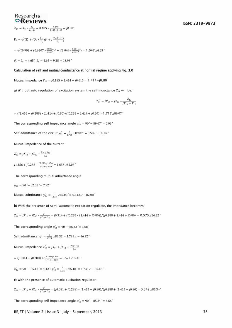
In determining the shunt resistance created by one phase short circuit to ground, the diagram of Fig. 4.0 will be applied for reverse

and zero sequences.

X1=0.531 X2=0.185 X =0.151 X =0.4255 7

X3=0.266 X4=0.145 X1k=0.151 X2k=0.425 X8=0.425

X9=j0.185ZL2=0.495+j0.215

Figure 4.0 System reverse sequence impedance diagram

For reverse sequence, load resistance is taken as 0.35Zload [2], therefore:

𝑍𝑙𝑜𝑎𝑑 2 = 0.35 ∗ 𝑍𝑙𝑜𝑎𝑑 = 0.35 ∗ 1.414 + 𝑗0.615 = 0.495 + 𝑗0.215

Rearranging the diagram of Fig. 4.0, it becomes:

𝑋14 =𝑗𝑋8

2=

𝑗0.425

2= 𝑗0.213

𝑋15 = 𝑋1″ + 𝑋2 ∗

𝑋3″ + 𝑋4

𝑋1″ + 𝑋2 + 𝑋3

″ + 𝑋4

= 0.31 + 0.185 0.266 + 0.145

0.31 + 0.185 + 0.266 + 0.145= 𝑗0.225

𝑍13 = 𝑗𝑋9 + 𝑍𝑙𝑜𝑎𝑑 2 = 𝑗0.185 + 0.495 + 𝑗0.215 = 0.495 + 𝑗0.40

Impedance transformation of figures 5 and 6

𝑍14 =𝑗𝑋15 ∗ 𝑍13

𝑗𝑋15 + 𝑍13

=𝑗0.225 0.495 + 𝑗0.40

𝑗0.225 + 0.495 + 𝑗0.40 = 0.039 + 𝑗0.175

𝑋16 = 𝑋5 ∗𝑋1𝑘

𝑋5 + 𝑋1𝑘 + 𝑋2𝑘

= 𝑗0.151 ∗𝑗0.045

𝑗0.151 + 𝑗0.106 + 𝑗0.045= 𝑗0.053

𝑋17 = 𝑋5 ∗𝑋2𝑘

𝑋5 + 𝑋1𝑘 + 𝑋2𝑘

= 𝑗0.023

𝑋18 = 𝑋1𝑘 ∗𝑋2𝑘

𝑋5+𝑋1𝑘+𝑋2𝑘= 𝑗0.016

ISSN: 2319-9873

RRJET | Volume 2 | Issue 3 | July – September, 2013 40

X15=j0.225 X5=j0.151 X14=j0.213

Z13=0.495+j0.40

X16 X17

X1k=j0.106

X18

X2k=j0.045

X15=j0.225 X5=j0.151 X14=j0.213

Z13=0.495+j0.40

X16 X17

X1k=j0.106

X18

X2k=j0.045

X15=j0.225 X5=j0.151 X14=j0.213

Z13=0.495+j0.40

X16 X17

X1k=j0.106

X18

X2k=j0.045

Figure 5.0 ∆/Y impedance conversion

Z15 X19

X18

K(1)

Figure 6.0 Resultant impedance from Figure 5

𝑍15 = 𝑍14 + 𝑗𝑋16 = 0.039 + 𝑗0.288

𝑋19 = 𝑋17 + 𝑗𝑋14 = 𝑗0.236

The equivalent impedance of the reverse sequence relative to the short circuit is Zeq.

𝑍𝑒𝑞 = 𝑗𝑋18 + 𝑗𝑋19 ∗𝑍15

𝑗𝑋19 +𝑍15= 𝑗0.016 +

𝑗0.236∗ 0.039+𝑗0.228

𝑗0.236+0.039+𝑗0.228= 0.01 + 𝑗0.133

X2=0.185 X20=0.453 X7 =0.425

X4=0.145 X21=0.317 X22=0.136 X8=0.425

K(1)

Figure 7.0 Zero sequence impedance diagram

For transmission lines, zero sequence reactance is defined as X0 = 3X1 [3]. Similarly, X20=3X5; X21=3X1k; X22=3X2k; X23=X2*X4/(X2+X4) =

0.0185*0.145/(0.0185+0.145) = j0.081

X24 = jX7/2 = j0.425/2 = j0.213 (Fig. 7.0).

X23 X20 X24

X25 X26

X21

X27

X22

K(1)

Figure 8.0 Conversion of ∆/Y impedance diagram

ISSN: 2319-9873

RRJET | Volume 2 | Issue 3 | July – September, 2013 41

𝑋25 = 𝑋20 ∗𝑋21

𝑋20 + 𝑋21 + 𝑋22

= 𝑗0.453 ∗𝑗0.317

𝑗0.453 + 𝑗0.317 + 𝑗0.136= 𝑗0.159

𝑋26 = 𝑋20 ∗𝑋22

𝑋20 + 𝑋21 + 𝑋22

= 𝑗0.453 ∗𝑗0.081

𝑗0.453 + 𝑗0.317 + 𝑗0.136= 𝑗0.068

𝑋27 = 𝑋21 ∗𝑋22

𝑋20 + 𝑋21 + 𝑋22

= 𝑗0.317 ∗𝑗0.136

𝑗0.453 + 𝑗0.317 + 𝑗0.136= 𝑗0.048

𝑋28 = 𝑋23 + 𝑋25 = 𝑗0.081 + 𝑗0.159 = 𝑗0.240

𝑋29 = 𝑋24 + 𝑋26 = 𝑗0.213 + 𝑗0.068 = 𝑗0.281

The equivalent reactance of the zero sequence relative to the point of short circuit K(1) is defined as:

𝑋𝑒𝑞 0 = 𝑋27 + 𝑋28 ∗𝑋29

𝑋28 + 𝑋29

= 𝑗0.048 + 𝑗0.24 ∗𝑗0.281

𝑗0.24 + 𝑗0.281= 𝑗0.177

The impedance of the power line at the point of short circuit is:

𝑍𝑠ℎ(1)

= 𝑗𝑋𝑒𝑞 (0) + 𝑍𝑒𝑞 = 𝑗0.177 + 0.01 + 𝑗0.133 = 0.01 + 𝑗0.31

Abnormal regime

Calculation of system reactance for single line-to-ground short circuit at15km distance from source.

X33 = X 1 + X2) ∗

X3 + X4

X2 + X2 + X3 + X4

=

0.531 + 0.185 ∗0.413 +0.145

0.531 +0.185+0.413+0.145= j0.80

Z16 = jX9 + Zload = j0.185 + 1.414 + j0.625 = 1.414 + j0.80

X1=0.531 X2=0.185 X =0.151 X =0.4255 7

X3=0.413 X4=0.145 X1k X2k X8=0.425

X30 X31

X32

X9ZL

Vs

E’

E’

Z’sh=0.01+j0.310

Figure 9.0 Abnormal regime impedance diagram

X30 = X5 ∗X1k

X5+X1k +X2k= j0.151 ∗

j0.1057

j0.151 +j0.1057 +j0.045= j0.053

X31 = X5 ∗X2k

X5+X1k +X2k= j0.027

ISSN: 2319-9873

RRJET | Volume 2 | Issue 3 | July – September, 2013 42

X32 = X1k ∗X2k

X5+X1k +X2k= j0.016

𝑍17 = 𝑍𝑠ℎ 1

+ 𝑋32 = 0.01 + 𝑗0.31 + 𝑗0.016 = 0.01 + 𝑗0.326

𝑋34 = 𝑗𝑋31 + 𝑗𝑋24 = 𝑗0.027 + 𝑗0.213 = 𝑗0.240

X33 X30 b X34

Z16 Z17

I(1) I(2) I(3)

I(5)

a

I(4)

E’

Figure 10.0 Equivalent generator circuit

Current quantity and its flow during abnormal regime Fig. 10

𝑉𝑠 = 0, 𝑎𝑛𝑑 𝐼 3 = 1.0∠0°

𝑉 𝑏 = 𝐼 3 ∗ 𝑗𝑋34 = 𝑗0.240; 𝐼 5 =𝑉 𝑏𝑍17

= 0.24∠90°/0.326∠88.24° = 0.736∠1.76°

𝐼 2 = 𝐼 3 + 𝐼 5 = 1.0 + 0.7357 + 𝑗0.0226 = 1.736 + 𝑗0.0226

𝑉 𝑎 = 𝑉 𝑏 + 𝐼 2 ∗ 𝑗𝑋30 = 𝑗0.24 + 1.736 + 𝑗0.0226 ∗ 𝑗0.053 = 0.332∠89.8°

𝐼 4 =𝑉 𝑎

𝑍16= (0.332∠89.8° ) (1.414 + 𝑗0.8) = 0.101 + 𝑗0.177 = 0.204∠60.3°

𝐼 1 = 𝐼4 + 𝐼 2 = 0.101 + 𝑗0.177 + 1.736 + 𝑗0.0226 = 1.848∠6.21°

Input emf 𝐸′ = 𝑉 𝑎 + 𝑗𝑋33 ∗ 𝐼1 = 0.332∠89.8° + 0.314∠90° ∗ 1.848∠6.21° = 0.911∠85.97°

Self impedance: 𝑍11″′ =

𝐸′

𝐼1= 0.911∠85.97°/1.848∠6.21° = 0.493∠79.76°

Self admittance angle: 𝛼11″′ = 90° − 79.76° = 10.24°

Self admittance: 𝑦11″′ =

1

0.493∠79.76°= 2.028∠ − 79.76°

𝑀𝑢𝑡𝑢𝑎𝑙 𝑖𝑚𝑝𝑒𝑑𝑎𝑛𝑐𝑒 𝑍12′″ =

𝐸′

𝐼3= 0.911∠85.97° ∗

1

1.0∠0° = 0.911∠85.97°

Mutual impedance angle: 𝛼12″′ = 90° − 85.97° = 4.03°

Mutual admittance: 𝑦12″′ =

1

0.911∠85.97°= 1.098∠ − 85.97°

Self and mutual reactance after accidental regime

X35=(X1+X2)(X3+X4)/(X1+X2+X3+X4)

𝑗0.531 + 𝑗0.185 ∗𝑗0.266+𝑗0.145

𝑗0.531+𝑗0.185+𝑗0.0.266+𝑗0.145 X36=jX5+X7/2 = j0.151+j0.425/2 = j0.364

Z18=jX9+Zload=1.414+j0.80, Fig. 11(b)

ISSN: 2319-9873

RRJET | Volume 2 | Issue 3 | July – September, 2013 43

X1=0.531 X2=0.185 X =0.151 X =0.4255 7

X3=0.413 X4=0.145 X8=X7

X9

E’

E’

= 0.185ZL=1.414+j0.625

Figure11(a) Reactances after accidental regime

E’ X35 X36

Z18

Figure11(b) Equivalent diagram after accidental regime

Self impedance: 𝑍11″ = 𝑗𝑋35 +

𝑗𝑋36∗𝑍18

𝑋36 +𝑍18= 0.634∠85°

Self admittance angle: 𝛼11″ = 90° − 85° = 5°

Self admittance: 𝑦11″ =

1

0.634∠85°= 1.577∠ − 85°

Mutual impedance: 𝑍12″ = 𝑗𝑋35 +

𝑗𝑋35∗𝑋36

𝑍18= 0.646∠84.6°

Self admittance angle: 𝛼12″ = 90° − 84.6° = 5.4°

Self admittance: 𝑦12″ =

1

0.646∠84.6°= 1.548∠ − 84.6°

Determination of maximum power at normal regime

(a) Without automatic excitation regulator on generator

𝑃𝑚1 = 𝐸𝑞2 ∗ 𝑦11

′ ∗ 𝑠𝑖𝑛𝛼11′ + 𝐸𝑞 ∗ 𝑉∗𝑠 ∗ 𝑦12

′ = 2.4552 ∗ 0.58 ∗ 𝑠𝑖𝑛0.93° + 2.455 ∗ 0.909 ∗ 0.612 = 1.4225

(b) With semi-automatic excitation regulator

𝑃𝑚2 = (𝐸′)2 ∗ 𝑦11′ ∗ 𝑠𝑖𝑛𝛼11

′ + 𝐸′ ∗ 𝑉∗𝑠 ∗ 𝑦12′ = 1.2372 ∗ 1.739 ∗ 𝑠𝑖𝑛3.68° + 1.237 ∗ 0.909 ∗ 1.733 = 2.1194

(c) With automatic excitation regulator

𝑃𝑚3 = 𝑉𝐺2 ∗ 𝑦11

′ ∗ 𝑠𝑖𝑛𝛼11′ + 𝑉𝐺 ∗ 𝑉∗𝑠 ∗ 𝑦12

′ = 1.0472 ∗ 2.942 ∗ 𝑠𝑖𝑛4.66° + 1.047 ∗ 0.909 ∗ 2.761 = 2.8881

6. Calculation of power characteristics at different regimes:

1) Maximum power at normal regime

𝑃𝑚′ = (𝐸′)2 ∗ 𝑦11

′ 𝑠𝑖𝑛𝛼11′ + 𝐸′ ∗ 𝑉∗𝑠 ∗ 𝑦12

′ sin(𝛿′ − 𝛼11′ )

= 1.2372 ∗ 1.739𝑠𝑖𝑛3.68° + 1.237 ∗ 0.909 ∗ 1.733 ∗ sin 𝛿′ − 4.42° = 0.171 + 1.949 ∗ sin 𝛿′ − 4.42° = 2.12

2) Maximum power at faulty regime

ISSN: 2319-9873

RRJET | Volume 2 | Issue 3 | July – September, 2013 44

𝑃𝑚″′ = (𝐸′)2 ∗ 𝑦11

″′ 𝑠𝑖𝑛𝛼11″′ + 𝐸′ ∗ 𝑉∗𝑠 ∗ 𝑦12

″′ sin(𝛿′ − 𝛼12″′ )

= 1.2372 ∗ 2.028𝑠𝑖𝑛10.24 + 1.237 ∗ 0.909 ∗ 1.098 ∗ sin 𝛿′ − 4.03° = 0.552 + 1.235 ∗ sin 𝛿′ − 4.03° = 1.787

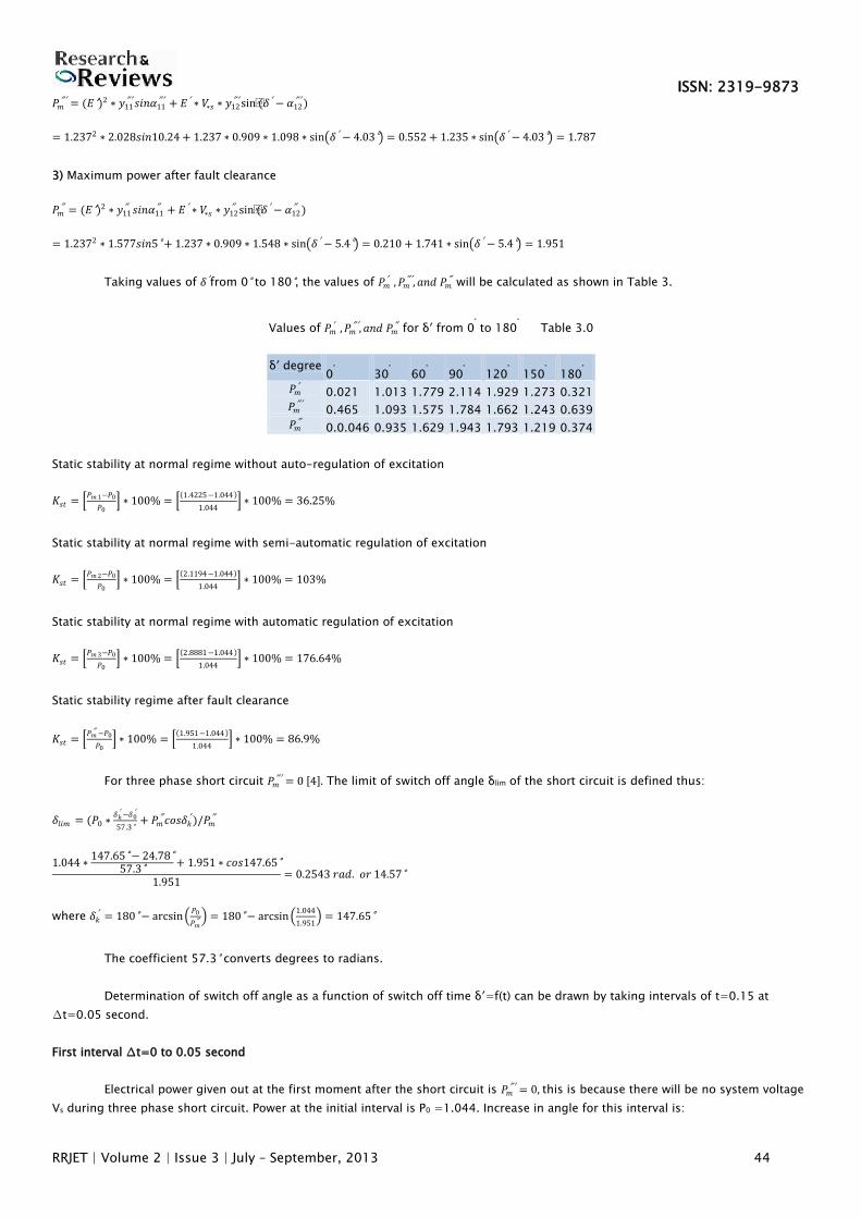
3) Maximum power after fault clearance

𝑃𝑚″ = (𝐸′)2 ∗ 𝑦11

″ 𝑠𝑖𝑛𝛼11″ + 𝐸′ ∗ 𝑉∗𝑠 ∗ 𝑦12

″ sin(𝛿′ − 𝛼12″ )

= 1.2372 ∗ 1.577𝑠𝑖𝑛5° + 1.237 ∗ 0.909 ∗ 1.548 ∗ sin 𝛿′ − 5.4° = 0.210 + 1.741 ∗ sin 𝛿′ − 5.4° = 1.951

Taking values of 𝛿′from 0° to 180°, the values of 𝑃𝑚′ , 𝑃𝑚

″′, 𝑎𝑛𝑑 𝑃𝑚″ will be calculated as shown in Table 3.

Values of 𝑃𝑚′ , 𝑃𝑚

″′, 𝑎𝑛𝑑 𝑃𝑚″ for δʹ from 0

° to 180

° Table 3.0

δʹ degree 0

° 30

° 60

° 90

° 120

° 150

° 180

°

𝑃𝑚′ 0.021 1.013 1.779 2.114 1.929 1.273 0.321

𝑃𝑚″′ 0.465 1.093 1.575 1.784 1.662 1.243 0.639

𝑃𝑚″ 0.0.046 0.935 1.629 1.943 1.793 1.219 0.374

Static stability at normal regime without auto-regulation of excitation

𝐾𝑠𝑡 = 𝑃𝑚 1−𝑃0

𝑃0 ∗ 100% =

1.4225−1.044

1.044 ∗ 100% = 36.25%

Static stability at normal regime with semi-automatic regulation of excitation

𝐾𝑠𝑡 = 𝑃𝑚 2−𝑃0

𝑃0 ∗ 100% =

2.1194−1.044

1.044 ∗ 100% = 103%

Static stability at normal regime with automatic regulation of excitation

𝐾𝑠𝑡 = 𝑃𝑚 3−𝑃0

𝑃0 ∗ 100% =

2.8881−1.044

1.044 ∗ 100% = 176.64%

Static stability regime after fault clearance

𝐾𝑠𝑡 = 𝑃𝑚

″ −𝑃0

𝑃0 ∗ 100% =

1.951−1.044

1.044 ∗ 100% = 86.9%

For three phase short circuit 𝑃𝑚″′ = 0 4 . The limit of switch off angle δlim of the short circuit is defined thus:

𝛿𝑙𝑖𝑚 = (𝑃0 ∗𝛿𝑘

′ −𝛿0′

57.3°+ 𝑃𝑚

″𝑐𝑜𝑠𝛿𝑘′ )/𝑃𝑚

″

1.044 ∗147.65° − 24.78°

57.3°+ 1.951 ∗ 𝑐𝑜𝑠147.65°

1.951= 0.2543 𝑟𝑎𝑑. 𝑜𝑟 14.57°

where 𝛿𝑘′ = 180° − arcsin

𝑃0

𝑃𝑚″ = 180° − arcsin

1.044

1.951 = 147.65°

The coefficient 57.3° converts degrees to radians.

Determination of switch off angle as a function of switch off time δ′=f(t) can be drawn by taking intervals of t=0.15 at

∆t=0.05 second.

First interval ∆t=0 to 0.05 second

Electrical power given out at the first moment after the short circuit is 𝑃𝑚″′ = 0, this is because there will be no system voltage

Vs during three phase short circuit. Power at the initial interval is P0 =1.044. Increase in angle for this interval is:

ISSN: 2319-9873

RRJET | Volume 2 | Issue 3 | July – September, 2013 45

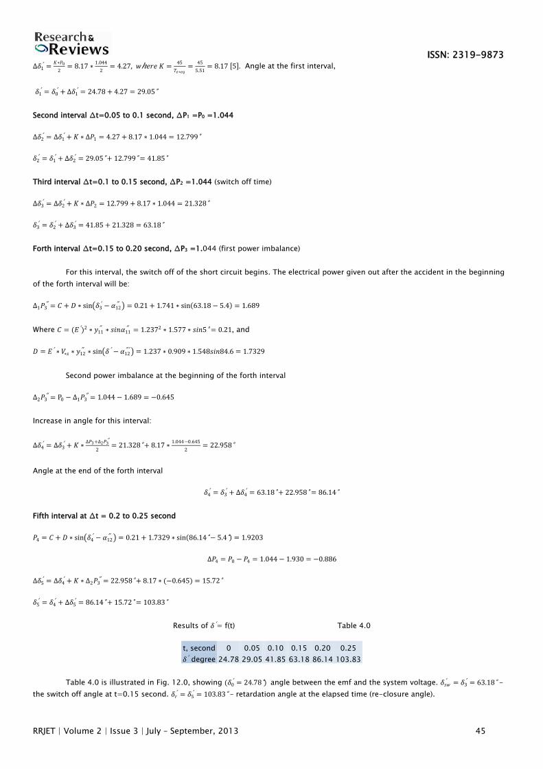
∆𝛿1′ =

𝐾∗𝑃0

2= 8.17 ∗

1.044

2= 4.27, 𝑤ℎ𝑒𝑟𝑒 𝐾 =

45

𝑇𝑒∗𝑒𝑞=

45

5.51= 8.17 5 . Angle at the first interval,

𝛿1′ = 𝛿0

′ + ∆𝛿1′ = 24.78 + 4.27 = 29.05°

Second interval ∆t=0.05 to 0.1 second, ∆P1 =P0 =1.044

∆𝛿2′ = ∆𝛿1

′ + 𝐾 ∗ ∆𝑃1 = 4.27 + 8.17 ∗ 1.044 = 12.799°

𝛿2′ = 𝛿1

′ + ∆𝛿2′ = 29.05° + 12.799° = 41.85°

Third interval ∆t=0.1 to 0.15 second, ∆P2 =1.044 (switch off time)

∆𝛿3′ = ∆𝛿2

′ + 𝐾 ∗ ∆𝑃2 = 12.799 + 8.17 ∗ 1.044 = 21.328°

𝛿3′ = 𝛿2

′ + ∆𝛿3′ = 41.85 + 21.328 = 63.18°

Forth interval ∆t=0.15 to 0.20 second, ∆P3 =1.044 (first power imbalance)

For this interval, the switch off of the short circuit begins. The electrical power given out after the accident in the beginning

of the forth interval will be:

∆1𝑃3″ = 𝐶 + 𝐷 ∗ sin 𝛿3

′ − 𝛼12″ = 0.21 + 1.741 ∗ sin 63.18 − 5.4 = 1.689

Where 𝐶 = (𝐸′)2 ∗ 𝑦11″ ∗ 𝑠𝑖𝑛𝛼11

″ = 1.2372 ∗ 1.577 ∗ 𝑠𝑖𝑛5° = 0.21, and

𝐷 = 𝐸′ ∗ 𝑉∗𝑠 ∗ 𝑦12″ ∗ sin 𝛿′ − 𝛼12

″′ = 1.237 ∗ 0.909 ∗ 1.548𝑠𝑖𝑛84.6 = 1.7329

Second power imbalance at the beginning of the forth interval

∆2𝑃3″ = P0 − ∆1𝑃3

″ = 1.044 − 1.689 = −0.645

Increase in angle for this interval:

∆𝛿4′ = ∆𝛿3

′ + 𝐾 ∗∆𝑃3+∆2𝑃3

″

2= 21.328° + 8.17 ∗

1.044−0.645

2= 22.958°

Angle at the end of the forth interval

𝛿4′ = 𝛿3

′ + ∆𝛿4′ = 63.18° + 22.958° = 86.14°

Fifth interval at ∆t = 0.2 to 0.25 second

𝑃4 = 𝐶 + 𝐷 ∗ sin 𝛿4′ − 𝛼12

″ = 0.21 + 1.7329 ∗ sin 86.14° − 5.4° = 1.9203

∆𝑃4 = 𝑃0 − 𝑃4 = 1.044 − 1.930 = −0.886

∆𝛿5′ = ∆𝛿4

′ + 𝐾 ∗ ∆2𝑃3″ = 22.958° + 8.17 ∗ (−0.645) = 15.72°

𝛿5′ = 𝛿4

′ + ∆𝛿5′ = 86.14° + 15.72° = 103.83°

Results of 𝛿′= f(t) Table 4.0

t, second 0 0.05 0.10 0.15 0.20 0.25

𝛿′ degree 24.78 29.05 41.85 63.18 86.14 103.83

Table 4.0 is illustrated in Fig. 12.0, showing (𝛿0′ = 24.78°) angle between the emf and the system voltage. 𝛿𝑠𝑤

′ = 𝛿3′ = 63.18° -

the switch off angle at t=0.15 second. 𝛿𝑟′ = 𝛿5

′ = 103.83° – retardation angle at the elapsed time (re-closure angle).

ISSN: 2319-9873

RRJET | Volume 2 | Issue 3 | July – September, 2013 46

P

2.0

1.0 Po

A p

A r

'00 'sw 'r 180,deg.

Figure 12.0 Generator swing curve

Speed up area Ap and possible retardation area Ar are defined in Fig. 13.0

𝐴𝑝 = 𝑃0 ∗𝛿𝑠𝑤

′ −𝛿0′

57.3°= 1.044 ∗

63.18°−24.78°

57.3°= 0.70

𝐴𝑟 = 𝑃0 ∗𝛿𝑘

′ −𝛿𝑠𝑤′

57.3°+ 𝑃𝑚

″ 𝑐𝑜𝑠𝛿𝑘′ − 𝑐𝑜𝑠𝛿𝑠𝑤

′ = 1.044 ∗147.65°−63.18°

57.3°+ 1.951 ∗ 𝑐𝑜𝑠147.65° − 𝑐𝑜𝑠63.18° = −0.9895

Reserved coefficient of dynamic stability of the power system (Kr) is defined as 𝐾𝑟 = |𝐴𝑟 |/𝐴𝑝 =−0.9895

0.7= 1.4136

P

1.0 Po

A p

0

A r1 A r2

P I I

P I

'0 'sw 'r 'r 180 ,deg. Figure 13.0 Dynamic stability curve

The influence of a successful auto-reclosure on the dynamic stability of the system has been presented. From table 4, it is

seen that reclosure angle 𝛿𝑟′ is equal to 103.83⁰ and reclosure time is 0.1second. Therefore, the retardation areas before Ar1 and Ar2

can be defined as stated below. These parameters can be used to define the coefficient of dynamic stability of the system through the

influence of auto-reclosure equipment installed on the power system.

𝐴𝑟1 = 𝑃0 ∗ (𝛿𝑟′ − 𝛿𝑠𝑤

′ ) ∗1

57.3+ 𝑃𝑚

″ 𝑐𝑜𝑠𝛿𝑟′ − 𝑐𝑜𝑠𝛿𝑠𝑤

′ = 1.044 ∗103 .83°−63.18°

57.3+ 1.951 ∗ 𝑐𝑜𝑠103.83° − 𝑐𝑜𝑠63.18° = −0.606

𝛿𝑘′ = 180° − arcsin(𝑃0 /𝑃𝑚

″) = 180° − arcsin(1.044/1.951) = 147.65°

𝐴𝑟2 = 𝑃0 ∗𝛿𝑘

′ −𝛿𝑟′

57.3+ 𝑃𝑚

′ ∗ 𝑐𝑜𝑠𝛿𝑘′ − 𝛿𝑟

′ = 1.044 ∗147.65°−103.83°

57.3°+ 2.12 ∗ 𝑐𝑜𝑠147.65° − 𝑐𝑜𝑠103.83° = −0.4858

Finally, the coefficient of dynamic stability of the system 𝐾𝑟 = |𝐴𝑟1 + 𝐴𝑟2| ∗1

𝐴𝑝=

0.606 +0.4858

0.70= 1.5597

CONCLUSION

As a result of the presence of automatic re-closure system on the power line, the re-closure angle was improved to 147.65⁰.

Consequently, the coefficient of dynamic stability was raised to 1.5597 as compared with the 1.4136 earlier obtained after fault

clearance. This result proves that the reserve of dynamic stability with auto re-closure in the system is more than when there is no

ISSN: 2319-9873

RRJET | Volume 2 | Issue 3 | July – September, 2013 47

auto re-closure system on the transmission line. Therefore, a successful automatic re-closure of transmission lines positively

influences the dynamic stability of power systems.

REFERENCES

1. Rodjkova LD, Kozulin VS. Electrical equipment of power stations and substations. M Energoatomizdat. 1987:141.

2. Ulianov SA. Electromagnetic transient processes in electrical systems. M. Energia, 1970.

3. Venikov VA. Transients in electromechanical processes in electrical systems. M. Vishaya Shkola, 1970.

4. Venikov VA. Transients in electromechanical processes in electrical systems. M. Vishaya Shkola, 1970.

5. Ulianov SA. Electromagnetic transient processes in electrical systems. M. Energia, 1970.