The inverse water wave problem of bathymetry detection

Under consideration for publication in J. Fluid Mech. 1

The inverse water wave problem ofbathymetry detection

VISHAL VASAN† AND BERNARD DECONINCK‡Department of Applied Mathematics, University of Washington

Seattle WA 98195-352420, USA

(Received 11 June 2012)

The inverse water wave problem of bathymetry detection is the problem of deducingthe bottom topography of the seabed from measurements of the water wave surface. Inthis paper, we present a fully nonlinear method to address this problem. The methodstarts from the Euler water wave equations for inviscid irrotational fluid flow, withoutany approximation. Given the water wave height and its first two time derivatives, wedemonstrate that the bottom topography may be reconstructed from the numerical solu-tion of a set of two coupled nonlocal equations. Due to the presence of growing hyperbolicfunctions in these equations, their numerical solution is increasingly difficult if the lengthscales involved are so that the water is sufficiently deep. This reflects the ill-posed na-ture of the inverse problem. A new method for the solution of the forward problem ofdetermining the water wave surface at any time, given the bathymetry, is also presented.

1. Introduction

The problem addressed in this paper is that of recovering the shape of the solid bound-ary bounding an inviscid, irrotational, incompressible fluid from measurements of the freesurface alone. This problem is an idealization of the ocean bathymetry detection problemwhich arises naturally in the study of coastal dynamics (Collins & Kuperman 1994; Grilli1998; Piotrowski & Dugan 2002; Taroudakis & Makrakis 2001). Further, knowledge of theocean bathymetry is crucial for safe underwater navigation. The current work considersfluid-mechanical principles to determine the shape and location of the bottom surface.Other approaches to the bathymetry detection problem exist (Collins & Kuperman 1994;Grilli 1998; Piotrowski & Dugan 2002; Taroudakis & Makrakis 2001). Perhaps the mostsignificant and popular ones are based on reflection of acoustic signals from the bottomsurface (Collins & Kuperman 1994; Taroudakis & Makrakis 2001). Other methods arebased on nonlinear properties of ocean waves such as variations in the dispersion relationof shoaling waves (Piotrowski & Dugan 2002) and further corrections to these formulas(Grilli 1998). A recent approach that takes into account the entire flow field is due toNicholls & Taber (2008). Their method is based on expansions of a nonlinear opera-tor that accounts for the bottom surface (the Dirichlet→Neumann operator or DNO).However, Nicholls & Taber (2008) restrict their approach to working with standing waveprofiles on the free surface. The extension to generic waves is not obvious.

The method we propose stands apart from the methods mentioned above in that wemake no assumptions on the nature of the free surface (such as small amplitude waves,standing waves, etc.). The method allows us to accurately recover the bottom surface fromonly measurements of the free-surface deviation from rest at several times. In particular,we can recover the average depth of the bottom surface i.e., we do not require this as input

† Email address for correspondence: [email protected]‡ Email address for correspondence: [email protected]

2 V. Vasan and B. Deconinck

as is required for linear and perturbative theories (Grilli 1998; Piotrowski & Dugan 2002)or by Nicholls & Taber (2008). Our approach is fully nonlinear and it is not limited to one-dimensional bottom surfaces. We assume the flow is periodic in the horizontal directionswithout the presence of a vertically uniform horizontal current. In other words, we assumethe velocity potential itself is periodic. Although the equations we derive are valid for one-and two-dimensional surface water-waves, the numerical examples presented are limitedto one-dimensional surfaces, due to the computational effort required to solve both theforward time-dependent evolution and the inverse bathymetry detection problem for two-dimensional surfaces.

The principal question we seek to address is that of what minimal input surface datais required to recover the bottom surface. In theory we have that, to recover the bot-tom surface the method of reconstruction requires the surface elevation and its first twoderivatives with respect to time as functions of the horizontal variable at one particularinstant of time. In practice, it suffices to require the surface elevation at several succes-sive instances of time as a function of the horizontal variable: the time derivatives maybe obtained through finite differences. Although the input requirements made in thiswork could be considered a challenge in and of themselves, advances in remote sensingtechnology suggest these are reasonable assumptions (Piotrowski & Dugan 2002).

The organization of this paper is as follows: Section 2 contains the derivation of theexact, nonlinear equations to be solved for the bottom surface. These equations are anecessary condition of the full set of equations modelling water waves. As a result, it ispossible to reconstruct large amplitude, nonlinear bottom surfaces from large amplitude,nonlinear free-surface deviations. In Section 3 we present several example calculationsof bottom surface recovery assuming the surface elevation and its first two derivativeswith respect to time as functions of the horizontal variable are provided. Following theexamples, in Section 4 we discuss in detail several numerical issues involved in the recon-struction of the bottom surface. Bathymetry detection is a challenging inverse problemand we delineate features of the method which exhibit the ill-posed character of theproblem. In short, many of the challenges can be explained by the fact that the velocityfield decays exponentially with depth for an inviscid, irrotational fluid. This behaviouris manifested mathematically through the presence of hyperbolic functions in the non-linear equations to be solved, whose exponential growth inhibits accurate representationin finite-precision arithmetic. Finally in Section 5, we repeat the examples of Section3 using finite-difference approximations of the time derivatives of the surface elevation.There we show that the bottom surface may be recovered from measurements of thesurface deviation from rest alone. The error introduced by the finite-difference approx-imation is negligible and the bottom surface is recovered accurately in certain parame-ter regimes, specifically in the shallow water regime. In this manuscript we recover thebottom surface from numerically generated free-surface elevations. Bathymetry recoveryfrom experimental data is not discussed.

In the appendices we present a re-derivation of the results of Ablowitz & Haut (2008)which leads to an alternate formulation of the water-wave problem. We adapt this for-mulation to solve the time-dependent evolution of water waves numerically in order toprovide the necessary input data for the bathymetry reconstruction. The forward prob-lem is of interest in its own right but we do not present the full details here. The purposeof the appendix is simply to illustrate the connections between the forward and inverseproblems as well as to give a flavour of our method for solving the forward problem. De-tails and more examples for the solution of the forward problem will appear in a futurepublication.

Inverse Bathymetry Problem 3

2. The bathymetry reconstruction equation

Euler’s Equations for the dynamics of an inviscid, irrotational periodic flow in a two(N = 1) or three (N = 2) dimensional domain D = {(x, z) ∈ RN × R : ζ < z < η, 0 <xi < Li, i = 1, . . . , N} are

∆φ+ φzz = 0, (x, z) ∈ D, (1a)

φz −∇ζ · ∇φ = 0, z = ζ(x), (1b)

φz −∇η · ∇φ = ηt, z = η(x, t), (1c)

φt +1

2

(|∇φ|2 + φ2

z

)+ gη = 0, z = η(x, t). (1d)

Here φ is the velocity potential, η is the surface displacement, g is the acceleration dueto gravity and Li is the period in the xi direction. We use the convention that theLaplacian and gradient refer to those in RN i.e., they refer to the horizontal Laplacianand horizontal gradient.

In this section we show how one can reconstruct the bottom topography ζ from onlymeasurements at the surface. In particular, we state what is meant by surface measure-ments. Ideally, this would entail a snapshot of η at some instant of time. However, thisis readily seen to be insufficient since Laplace’s Equation has a unique solution for everyη and ζ suitably smooth, with prescribed boundary conditions. On the other hand, ifwe are given the complete solution of the free-boundary value problem (1a-1d) then thisis (by definition) sufficient information. Our definition of surface measurements lies inbetween these two extremes: we require η(x, t0), ηt(x, t0) and ηtt(x, t0), i.e., the surfacedeviation from the undisturbed level and its first two t−derivatives as functions of thehorizontal variable at one particular instant t = t0. The following paragraphs indicatewhy this is the case. The functions η(x, t0), ηt(x, t0) and ηtt(x, t0) can be considered thefirst three terms of the Taylor series of η(x, t) at some time t = t0 and hence representindependent pieces of information. Note that equation (1c) implies ηt(x, t0) is the normalvelocity of the fluid at z = η(x, t).

If we are given the surface quantities η(x, t) and q = φ(x, η), the Hamiltonian formu-lation of the water-wave problem due to Zakharov (1968) indicates that these surfacequantities fully determine the solution to the water-wave problem (1a-1d). Instead, fornow assume that at some instant of time t0 the velocity potential at the surface q(x, t0),the shape of the surface η(x, t0) and the normal velocity ηt(x, t0) are given. This is suf-ficient information to pose the following initial-value problem for the Laplace Equationwith periodic boundary conditions in the horizontal directions:

∆φ+ φzz = 0, z < η, (2a)

φz −∇η · ∇φ = ηt, z = η, (2b)

φ = q, z = η. (2c)

The question of bottom topography reconstruction involves finding a surface ζ such that(1b) is satisfied by the solution of the above problem. Several issues arise. First, we wantto obtain an exact expression for the solution of (2a-2c) in terms of known quantities sothat (1b) becomes a (nonlinear) equation for the unknown bottom surface ζ. Indeed solv-ing the initial-value problem for the Laplace Equation is numerically challenging. Second,the general initial-value problem (in z) for the Laplace Equation may not have a solutionfar from z = η(x, t0). The Cauchy-Kowalevski Theorem (Evans 1998) only guarantees asolution in the neighbourhood of the initial condition i.e, near z = η(x, t0). However, thetrue bottom surface ζ may be outside of this neighbourhood. Third, measurements of


the velocity potential at the surface q(x, t0) are impractical compared to measurementsof the surface elevation itself and it is desirable to eliminate q(x, t0) from the problem.We proceed to address these issues below.

The expression

φ =q̂ (0)

(2π)N+

1

(2π)N

∑k∈Λ

eik·x cosh(|k|z)q̂ (k) +1

(2π)N

∑k∈Λ

eik·xsinh(|k|z)|k|

η̂t(k), (3)

is a formal solution of (2a-2c) when η(x, t0) ≡ 0. Here q̂ (k) and η̂t(k) are the Fouriertransforms of q(x, t0) and ηt(x, t0) respectively. Thus

q̂ (k) =

∫R

e−ik·xq(x)dx, η̂t(k) =

∫R

e−ik·xηt(x)dx,

where

R = {x ∈ RN : 0 < xi < Li, i = 1, . . . , N}is the horizontal domain. The summation in (3) extends over all k in the lattice dual tothe physical period lattice, but disregards the zero mode. Hence

Λ =

{[2πn1

L1,

2πn2

L2

]T: nj ∈ Z, n2

1 + n22 > 0

},

see Deconinck & Oliveras (2011) for details.To find ζ, evaluate the left-hand side of equation (1b) using (3) for φ. This results

in the nonlinear function whose zero is the surface ζ. If the given Cauchy data (theDirichlet data q(x, t0) and the Neumann data ηt(x, t0)) are consistent with a well-posedboundary-value problem for Laplace’s Equation (for instance a Dirichlet condition atz = 0 and the Neumann condition (1c) at z = ζ), then the solution exists outside of asmall neighbourhood of the surface z = 0. For the specific form of the solution (3) to bevalid at z = ζ we require additional hypotheses. In particular, the true bottom boundaryshould be analytic and thus be well approximated by bounded sets in Fourier space.

The expression (3) for φ may be generalized to η(x, t0) = h0 where h0 is a constant.Fourier transform methods are cumbersome when initial conditions are given on surfaces,as in (2a-2c). Therefore we reduce this initial-value problem to a problem posed onz = −h0.

The reformulation of the water-wave problem due to Ablowitz, Fokas & Musslimani(2006) introduces a global relation for the Laplace Equation. The global relation connectsthe boundary information on the surface η and on the bottom topography ζ. We limitourself to applying the nonlocal relation of Ablowitz et al. (2006) on the region −h0 <z < η(x, t0). This allows us to transfer the data on z = η(x, t0) to equivalent data onz = −h0.

Let φ be a harmonic function in 0 < xi < Li, −h0 < z < η, periodic in the horizontalvariables xi with period Li. Following Ablowitz et al. (2006),

∇ ·FH +∂FV

∂z= 0,

where

FH = (−ikφz + ω∇φ)E,

FV = (ωφz + ik·∇φ)E,

with E = exp(−ik · x+ωz) and ω = ±|k|. Integrating this divergence form and applying


Green’s Theorem we obtain the global relations∫R

e−ik·x+|k|η [|k|(−∇φ·∇η + φz) + ik·(∇φ+ φz∇η)]z=η dx

=

∫R

e−ik·x−|k|h0 [|k|(−∇φ·∇η + φz) + ik·(∇φ+ φz∇η)]z=−h0dx, (4)

and ∫R

e−ik·x−|k|η [−|k|(−∇φ·∇η + φz) + ik·(∇φ+ φz∇η)]z=η dx

=

∫R

e−ik·x+|k|h0 [−|k|(−∇φ·∇η + φz) + ik·(∇φ+ φz∇η)]z=−h0dx. (5)

Using

[φz −∇φ · ∇η]z=η = ηt,

and

[∇φ+ φz∇η]z=η = ∇q,where ηt(x, t0) and q(x, t0) are the Neumann and Dirichlet values imposed at z = η(x, t0),we may rewrite the global relations (4) and (5) as∫

R

e−ik·x+|k|η [|k|ηt + ik·∇q] dx =

∫R

e−ik·x−|k|h0 [|k|ϕz + ik·∇ϕ] dx, (6)∫R

e−ik·x−|k|η [−|k|ηt + ik·∇q] dx =

∫R

e−ik·x+|k|h0 [−|k|ϕz + ik·∇ϕ] dx. (7)

where ϕ = φ(x,−h0). Multiplying (6) by e|k|h0 and (7) by e−|k|h0 , we can solve for theterms on the right-hand side to obtain∫

R

e−ik·xϕzdx =

∫R

e−ik·x[cosh(|k|(η + h0))ηt + i

sinh(|k|(η + h0))

|k|k·∇q

]dx, (8)

−∫R

e−ik·xϕdx =

∫R

e−ik·x[

sinh(|k|(η + h0))

|k|ηt + i

cosh(|k|(η + h0))

|k|2k·∇q

]dx. (9)

In order to obtain the above equations, we impose that φ is periodic. In other words, weassume there is no mean current. This assumption is made throughout the present work.

Let us take a moment to discuss what we have accomplished. A well-posed problem forLaplace’s Equation is a boundary-value problem, not a Cauchy-problem. Given data atboth z = η(x, t0) and z = −h0, we may employ the above global relations to solve for theremaining unknown boundary conditions. Green’s integral representation for a harmonicfunction in terms of its boundary data provides a solution to Laplace’s Equation. Thissolution depends continuously on the given boundary information, see Evans (1998). Forthe problem of bathymetry reconstruction, we are given information only on the surfacez = η(x, t0) and hence we need to solve the Cauchy problem (an initial-value problem)which is well known to be ill-posed (Evans 1998; Guenther & Lee 1996). However, withthe knowledge that our input data comes from a well-posed boundary-value problemand that the domain of harmonicity extends at least to z = −h0, the global relationallows us to transfer the given information at z = η to that at z = −h0. Consequently,we have evaluated the harmonic function in the interior of the domain. Since harmonicfunctions are analytic in the interior of their domain of definition (and hence their Fouriertransform decays exponentially as a consequence of a Paley-Wiener-type theorem (seePaley & Wiener 1934)), the Cauchy problem can be solved off the line z = −h0.


The discussion in the previous paragraph suggests that the definition:

φ(x, z) =ϕ̂(0)

(2π)N+

1

(2π)N

∑k∈Λ

eik·x cosh(|k|(z + h0)) ϕ̂

+1

(2π)N

∑k∈Λ

eik·xsinh(|k|(z + h0))

|k|ϕ̂z , (10)

is reasonable, and further that φ is harmonic in a neighbourhood of z = −h0. In particularwe may look for a surface ζ on which φ satisfies a homogeneous Neumann condition usingthis definition. Hence we consider

F (ζ) = [φz −∇ζ · ∇φ]z=ζ(x) , (11)

where φ is given by (10). We have obtained a nonlinear function of ζ whose zero impliesthe bottom-boundary condition (1b) is satisfied. If we find such a ζ, then existence-uniqueness results for the Laplace Equation, and the water-wave problem in particular(Lannes 2005; Wu 2011), imply we have recovered the bottom topography. Notice how-ever, that the numerical evaluation of the above expression for F is a formidable task.Considerable care must be taken in evaluating the hyperbolic functions. The exponentialgrowth of such terms in (10) can cause numerical errors leading to errors in the overallsolution.

Before proceeding, we highlight a subtlety regarding notation in (10). We use the hatnotation to indicate Fourier transform. In equation (10) we take the Fourier transform

of ϕz. This will be our convention throughout. Thus ∇̂ϕ refers to the Fourier transformof the gradient of ϕ i.e., the hat extends over the gradient symbol.

Remark 2.1. Under the assumption of the existence of h0 such that

minxη > −h0 > max

xζ,

equation (10) is an equally effective starting point for a boundary-value problem forLaplace’s Equation. Indeed, enforcing the given boundary conditions at z = η and z = ζ,we have two equations for the two unknowns ϕ̂z and ϕ̂. The right-hand side of (10) maybe interpreted as a sum of linear operators acting on ϕ̂z and ϕ̂. Solving this system ofequations effectively requires “dividing” by the hyperbolic terms. It is precisely this inver-sion that leads to the smoothness of the harmonic function in the interior as well as thewell-posedness of the boundary-value problem. See Appendix B for further details regard-ing boundary-value problems for Laplace’s Equation and the forward problem of the timeevolution of a water wave.

The nonlinear function F defined in (11) depends on both the Neumann and Dirichletdata at the surface z = η(x, t0). We may treat the Dirichlet data as an unknown if wecan supplement the equation (11) with another. Indeed, recall condition (1b) holds forall time. Hence we consider the following system of nonlinear equations for ζ and q:

F (ζ, q) = [φz −∇ζ · ∇φ]z=ζ(x) = 0,

d

dtF (ζ, q) =

d

dt

([φz −∇ζ · ∇φ]z=ζ(x)

)= 0,

(12a)

(12b)


where

∇φ(x, z) =∑k∈Λ

ikeik·x(

cosh(|k|(z + h0))ϕ̂+sinh(|k|(z + h0))

|k|ϕ̂z

),

=∑k∈Λ

eik·x(

cosh(|k|(z + h0))∇̂ϕ+ik

|k|sinh(|k|(z + h0))ϕ̂z

), (13)

and

φz(x, z) =∑k∈Λ

eik·x (|k| sinh(|k|(z + h0))ϕ̂+ cosh(|k|(z + h0))ϕ̂z) ,

=∑k∈Λ

eik·x(− ik|k|

sinh(|k|(z + h0))∇̂ϕ+ cosh(|k|(z + h0))ϕ̂z

). (14)

The fluid velocities at z = −h0 (the tilde variables) are given in terms of surface mea-surements by

ϕ̂z =

∫R

e−ik·x[cosh(|k|(η + h0))ηt + i

sinh(|k|(η + h0))

|k|k·∇q

]dx, (15)

∇̂ϕ =

∫R

e−ik·x[−ik|k|

sinh(|k|(η + h0))ηt + cosh(|k|(η + h0))k

|k|2k·∇q

]dx. (16)

Finally, we supplement these equations with the time derivative of the surface velocitypotential, namely

qt = −gη − 1

2|∇q|2 +

(ηt +∇q · ∇η)2

2(1 + |∇η|2),

which is the equation of evolution for the surface potential obtained by Ablowitz et al.(2006). As the velocity potential at the surface only appears through its spatial deriva-tives, we solve equations (12a) and (12b) for the unknowns ζ and ∇q.

Examining equation (12b), we observe that at some instant of time, we require thesurface displacement η(x, t0), the normal velocity ηt(x, t0) and its rate of change ηtt(x, t0)as functions of the horizontal variable x. Figure 1 provides an overview of the algorithm toreconstruct the bottom boundary. Assume we are given the Dirichlet (rather its gradienti.e., the tangential derivative of the velocity potential) and Neumann data (the normalvelocity ηt(x, t0)) at the surface z = η(x, t0). We use the AFM global relation to convertthis data to corresponding data at some height z = −h0. Using the information at thehorizontal line z = −h0, we solve the initial-value problem for Laplace’s Equation in thevertical direction (along z). Finally we look for a surface z = ζ such that the normalderivative of the potential (obtained through solving the initial-value problem) along thesurface vanishes. Thus we have evaluated the nonlinear function F in equation (12a)assuming we know q(x, t0). However, as the boundary condition (1b) holds for all time,we impose relation (12b). This allows us to eliminate the Dirichlet data at z = η(x, t0).Although the presentation above is valid for N = 1, 2, we restrict ourselves to N = 1 forthe rest of the discussion.

Remark 2.2. As shown by Lannes (2005) and Wu (2011), the water-wave problem(1a-1d) is well posed and has a unique solution. Since the set of nonlinear equations(12a-12b) are necessary conditions for the full water-wave problem, existence of solutionsto these nonlinear equations is guaranteed. We do not investigate uniqueness of solutionsto these equations.


Use data here...

...to get data here.

Solve Laplace's equation"off" this line.

Evaluate the solution along a curve

1

23

4

Figure 1. Algorithm for reconstruction of the bottom surface.

3. Examples

In this section we present example reconstructions carried out using the method pro-posed in the previous section. In all the examples discussed below, the input data isobtained from the non-dimensional version of equations (1a-1d). Assuming the scaling

φ = l√glφ∗, η = lη∗, z = lz∗, x = lx∗, t =

√l

gt∗, (1)

where l = L/(mπ), m is a positive integer and L is the period in the horizontal direction,we have the following non-dimensional form of equations (1a-1d) for N = 1:

φxx + φzz = 0, (x, z) ∈ D, (2a)

φz − ζxφx = 0, z = ζ(x), (2b)

φz − ηxφx = ηt, z = η(x, t), (2c)

φt +1

2

(φ2x + φ2

z

)+ η = 0, z = η(x, t). (2d)

Here D = {(x, z) ∈ R2 : ζ < z < η, 0 < x < mπ} and we have dropped the superscriptstars. To distinguish the different regimes of the fluid flow (i.e., shallow water, largeamplitude, etc.) we define the quantities

µ =|ζ|mπ

, ε = maxx

∣∣∣ηh

∣∣∣ , h =1

mπ

∫ mπ

0

ζdx.

Thus the larger ε (the amplitude parameter) is, the more nonlinear the fluid flow is.Values of µ near 1 indicate deep water, whereas smaller values indicate shallow water.Note that µ is a function of the spatial variable x.

To solve equations (12a-12b) numerically, we approximate both unknowns ζ and qx bytheir truncated Fourier series

ζ =

Kζ∑k=−Kζ

eikxζ̂k, qx =

Kqx∑k=−Kqx

eikxq̂x.

Here Kζ and Kqx define the resolution of the series for the bottom surface and thetangential velocity at the free surface η, respectively. The input data to the nonlinear


equations (12a-12b) are η, ηt and ηtt as functions of x at one particular time t0. Typicallyη, ηt are obtained from a simulation of the time-dependent evolution of water waves withKη the highest wavenumber resolved in the horizontal direction. Thus the incoming datahas a maximum resolution corresponding to Kη. The generic inverse problem requiresηtt to be provided as well. In such cases, ηtt(x, t0) is computed from ηt(x, t0) using afive-point finite-difference stencil.

The expressions in (13) and (14) involve summations over all wavenumbers. Thesesummations are truncated with highest mode number Kφ during the computations. Thenonlinear functions are evaluated at several points in the physical grid and the prob-lem is solved as a least-squares problem with the Fourier modes of the bottom surfaceand tangential velocity as the parameters. We use MINPACK’s implementation of theLevenberg-Marquardt algorithm as the least-squares solver.

3.1. Flat bottom reconstruction using travelling wave solutions

As a first example, consider the case of a travelling wave solution of Euler’s Equations.The exact nonlinear travelling wave solutions corresponding to a particular value of thespeed c are obtained from the work of Deconinck & Oliveras (2011). Given the surfaceprofile η, computing ηt and ηtt is straightforward once the travelling wave assumption ismade. However, in this special case we know that the tangential velocity at the surfaceis related to the surface profile η through

qx = c−√

(c2 − 2gη)(1 + η2x),

as described in Deconinck & Oliveras (2011). Consequently, the second equation (12b)is not required for the bottom surface reconstruction. This dramatically reduces thecomputational effort. Furthermore, the bottom surface in the case of a travelling waveis known to be flat (for otherwise the bottom boundary ζ must be time-dependent) andwe are in search of a single mode for the bottom surface. One can attempt to find thezero of the norm of the nonlinear function (12a). However we minimize the full functionevaluated at various grid points in the horizontal variable. In fact, we do not assume thebottom surface to be flat, i.e., we assume the bottom surface is parametrized by severalmodes, as in the general case.

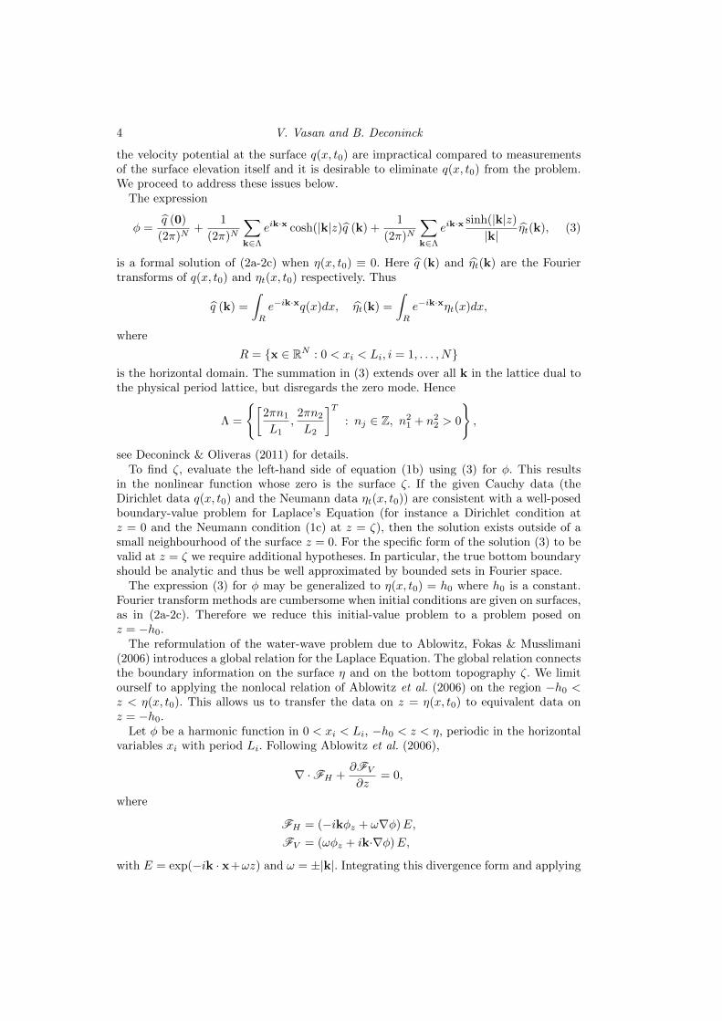
Figure 2 depicts a 2π-periodic travelling-wave solution (bold solid line) with

max |η| = 0.001.

The true bottom boundary is given by ζ = −0.1 and the speed of the wave c =0.31641443. Thus ε = 0.01 and µ = 0.016. The initial guess for the bottom surfaceis shown as a dashed line. As mentioned earlier, the bottom surface is not assumed tobe uniform. The true bottom surface is given by the thin solid line whereas the big dotsindicate the reconstructed bottom surface evaluated at select points. Because of the dif-ference in magnitude of the free surface and bottom topography, we have used dual axes.The relative error in the reconstructed solution is O(10−10). Note that all modes exceptthe zero mode are reduced in magnitude from their initial value. Indeed, in our method,the solution converges precisely to the bottom surface without any a priori knowledgeof the average depth. This is in contrast to other methods based on water-wave motionthat have been suggested in the literature, for instance, that of Nicholls & Taber (2008).

3.2. Flat bottom reconstruction using non-stationary waves

Using non-stationary waves, both equations (12a) and (12b) must be solved simultane-ously. In this section we present the reconstruction of a flat bottom, as in the previousexample. When the surface η and normal velocity ηt are given, we are able to reconstruct


0 1 2 3 4 5 6

0.003

0.002

0.001

0.000

0.001

0.002

η

0.15

0.10

0.05

0.00

0.05

ζ

Figure 2. Flat bottom reconstruction using traveling wave solutions. Note the dual axes forthis figure. The free surface η is shown with the solid bold line (with axis on the left). The truebottom surface and the reconstructed surface are shown in solid and dotted lines respectively,with the axis on the right. Here the initial guess for the least-squares solver is shown by thedashed line above.

0 2 4 6 8 10 12

0.10

0.05

0.00

0.05

0.10

(a) t = 0.5

0 2 4 6 8 10 12

0.10

0.05

0.00

0.05

(b) t = 1.0

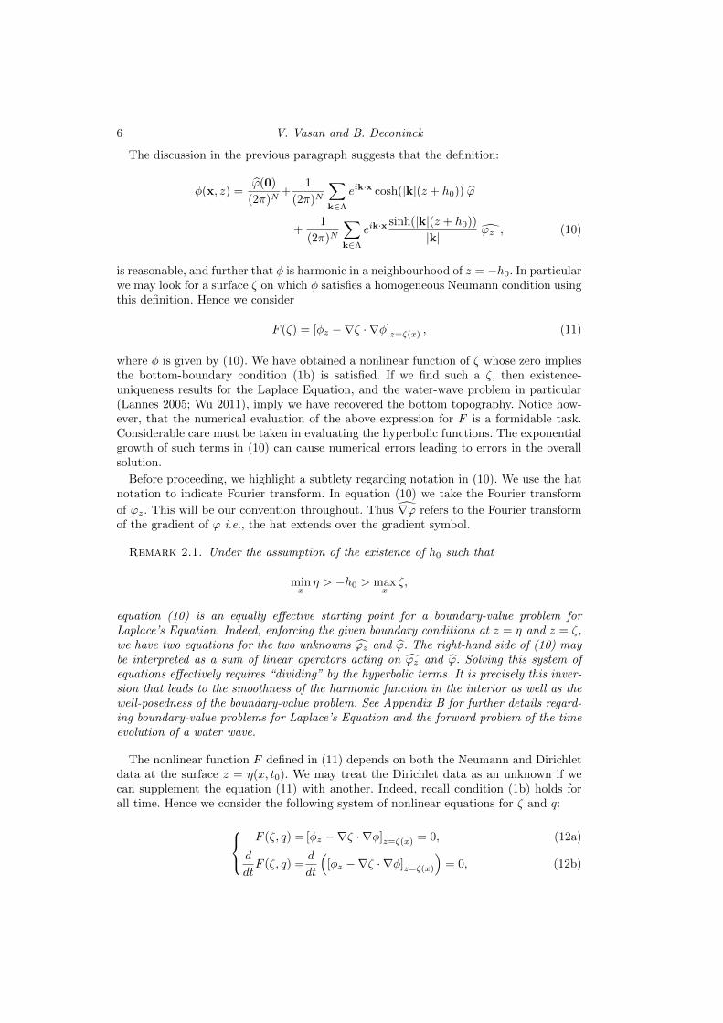
Figure 3. Reconstructing the flat bottom using non-stationary flow. The bold solid line showsthe free surface η, the dashed line is the initial guess and the dotted line depicts the final solution.The true solution is shown by the thin solid line. The true bottom surface and the reconstructionare indistinguishable on the scale of the figure.

the flat bottom of ζ = −0.1. At times t = 0.5 and t = 1.0 (figure 3), the relative errorin the tangential velocity at the surface is O(10−8) and the relative error in the recon-struction of the bottom surface is O(10−9). The shallowness parameter µ for these casesis 0.008 and ε = 1.25 based on the initial condition for the forward problem. Thus theinput data corresponds to very nonlinear flow in shallow water. Typically, both tangentialvelocity and bottom surface need to be well resolved to obtain a zero for the nonlinearfunctions (12a-12b).

Figure 4 depicts the reconstruction of the same flat surface, but at a later time. Asseen in (4b), the normal velocity and its time rate of change are sharply peaked. Thiscreates some numerical challenges when the fluid velocities at z = −h0 (15-16) arecomputed using the same number of Fourier modes as are used for the surface quantities.To allow the least-squares solver to converge we need to smooth the data at z = −h0 byreducing Kφ appropriately. On truncating the modes, the solver converges to the truesolution. Without truncation (Kφ = Kη), the least-squares routine converges, however


0 2 4 6 8 10 12

0.10

0.08

0.06

0.04

0.02

0.00

0.02

0.04

(a) t = 2.

0 2 4 6 8 10 120.2

0.1

0.0

0.1

0.2

(b) ηt (solid) and ηtt (dashed) vs. x at t = 2.

Figure 4. Reconstructing a flat bottom from non-stationary flow. Figure 4a is the same asfigure 3 but at t = 2. Notice the sharply peaked spatial profiles of ηt and ηtt in figure 4b whichposes difficulty in bottom surface reconstruction.

the nonlinear function has non-zero norm at the solution. This and other numerical issuesare discussed in detail in Section 4.

3.3. x−dependent bathymetry

In this section we present the recovery of more complicated bottom surfaces. The firstexample is of a surface that is approximated well by a finite number of Fourier modeswhereas the remaining examples require a large number of modes to be well approxi-mated. In all cases we solve both equations (12a) and (12b) using a least-squares routineassuming the knowledge of η(x, t0) and ηt(x, t0) (obtained from a simulation of the time-dependent forward problem).

3.3.1. High-frequency wavy bottom

The bottom surface

ζ = −0.2− (0.01 sin 2x+ 0.025 sinx cos 2x+ 0.01 sin 12x) , (3)

represented by a finite number of Fourier modes, is recovered using data from a simulationof the forward problem. The shallowness parameter varies between 0.0134 and 0.0183whereas ε is roughly 0.3 indicating moderate amplitude waves in shallow water. Here wepresent results from one instance t0, but it should be noted that the same surface maybe recovered from data at any instance. Figure 5 presents the bottom surface recoveredfor fixed Kqx and increasing Kζ . As seen from Figures 5a-5d, the bottom surface isprogressively better approximated with increasing Kζ . As Kζ is increased, the norm ofthe nonlinear functions in (12a-12b) decreases, providing a check for convergence to thetrue solution. Figures 5e-5f show the bottom surface and tangential velocity at the free-surface for a suitably large value of Kqx . The relative error in either the reconstructed ζand qx is O(10−9). Note that we also recover the zero mode of the bottom surface fromthe least-squares computation.

3.3.2. A Gaussian bump

Our next example is the recovery of a localized feature on an otherwise flat bottom-surface. The bottom surface is given by

ζ = −0.2 + 0.025e−(x−mπ/2)2 . (4)


0 2 4 6 8 10 12

0.20

0.15

0.10

0.05

0.00

0.05

(a) Kζ = 4, Kqx = 48

0 2 4 6 8 10 12

0.20

0.15

0.10

0.05

0.00

0.05

(b) Kζ = 8, Kqx = 48

0 2 4 6 8 10 12

0.20

0.15

0.10

0.05

0.00

0.05

(c) Kζ = 10, Kqx = 48

0 2 4 6 8 10 12

0.20

0.15

0.10

0.05

0.00

0.05

(d) Kζ = 12, Kqx = 48

0 2 4 6 8 10 12

0.20

0.15

0.10

0.05

0.00

0.05

(e) Kζ = 12, Kqx = 62

0 2 4 6 8 10 12

0.04

0.02

0.00

0.02

0.04

(f) Kζ = 12, Kqx = 62

Figure 5. Bottom surface reconstruction with different resolutions. Figures 5a-5e depict thereconstructed surface (dots) and the true bottom surface (thin solid line) for different resolutions.The free surface is depicted by the solid bold line. Figure 5f shows the computed (dots) and true(solid) tangential velocity at the free surface.

A localized feature such as a Gaussian is well represented in Fourier space by a suit-ably large number of modes. Consequently, as seen in figure 6, Kζ = 8 is sufficient torecover the bottom surface accurately. The reduced amplitude in the surface deviation(as compared to the previous example, here ε = 0.03) implies that large values of Kqx

are not required. Figure 6c is a plot of the relative error in the bottom surface ζ (dots)


0 2 4 6 8 10 12

0.20

0.15

0.10

0.05

0.00

(a) Computed and true bottom surface

0 2 4 6 8 10 12

0.004

0.002

0.000

0.002

0.004

(b) Computed and true tangential velocity atfree-surface

0 5 10 15 20 2510-10

10-8

10-6

10-4

10-2

(c) Relative error vs. Kζ for the bottom to-pography ζ shown in dots and for the tan-gential velocity at the free surface qx shownin asterisks.

Figure 6. Reconstruction for the case of a Gaussian bump on bottom surface (4) with Kζ = 8,Kqx = 24. Figures 6a-6b show the true solution (thin solid line) and the computed solution(dots). The bold solid line in figure 6a indicates the free surface η.

and the tangential velocity at the free-surface qx (asterisks) versus Kqx . We see a similarconvergence to the true solution as Kqx increases. Larger values of Kqx do not result inany further reduction in the relative error. Possible reasons for this are discussed in thenext section.

3.3.3. A sandbar

Consider the bottom surface given by

ζ = −0.1 + 0.015 tanh(3(x− 0.3L)) + 0.015 tanh(3(x− 0.7L)), (5)

which models a sandbar. Figure 7a presents recovery of this profile (shown with dots) andthe true bottom surface (solid line). The free surface (bold solid line) and initial guess forthe bottom surface (dashed line) are shown for reference. Alongside, in figure 7b, we seethe mode-by-mode relative error (dashes) between the computed bottom surface (dots)and the true bottom surface (solid line). As expected, the relative error is largest formodes with smallest amplitude. The overall relative error for the bottom surface in theinfinity-norm is O(10−7) and in the 2-norm is O(10−8).


0 2 4 6 8 10 12

0.02

0.02

0.06

0.10

(a)

5 10 15 20 25 30 35

10-13

10-9

10-5

10-1

103

(b)

Figure 7. Reconstruction of a sandbar profile. Figure 7a compares the true (thin solid) andcomputed (dots) bottom surfaces. Figure 7b is a mode-by-mode comparison of the amplitudein Fourier space of the true (solid line) and computed solution (dots). The dashed line indicatesthe relative error in the amplitude of each mode.

0 10 20 30 40 50 60 7010-8

10-7

10-6

10-5

10-4

10-3

10-2

Figure 8. Amplitude of Fourier modes for the multi-feature bottom surface (6).

3.3.4. A multi-feature bottom surface

Our final example consists of recovering a more complex bottom surface consisting oftwo distinct isolated features: a smooth step and a ripple patch. The exact surface isgiven by

ζ =− 0.2 + 0.02 tanh 10(x−mπ/8)− 0.02 tanh 10(x−mπ/4)

+ 0.02 cos 6x (tanh 10(x− 7mπ/8)− tanh 10(x− 3mπ/4)) . (6)

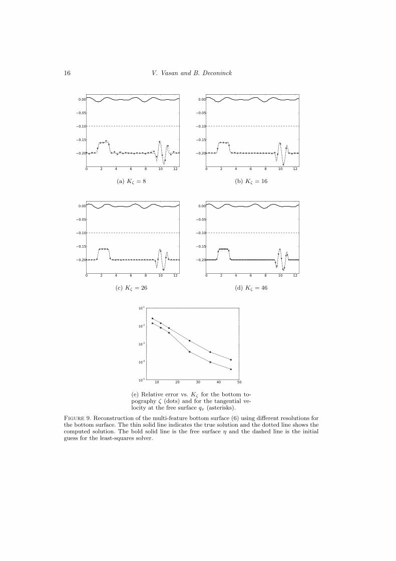
Figure 9 shows results for the bottom surface recovery for increasing values of Kζ . Thestep-like condition requires a large number of Fourier modes, particularly to resolvethe flat plateau between the features. Indeed the largest error is observed along the flatsurface. Note the increased relative error in recovery of the bottom surface as compared tothe other examples. The increased error is in part due to the fact that the bottom surfaceis not fully resolved in the forward simulation. The amplitudes of the Fourier modes of thebottom surface used in the forward simulation are shown in figure 8. Ideally, the largestmode resolved should have an amplitude on the order of machine precision (which is 10−15

for these calculations). As a result, the Hamiltonian for the time-dependent evolution ofthe water waves has a relative error of O(10−6) compared to the desired O(10−15) forthe other simulations. In effect, this example illustrates the reconstruction of the bottom


surface from data that is not an accurate solution to the water-wave problem. Of course,there are many issues to be separated before we can conclusively establish reconstructionfrom erroneous data. Nevertheless, this example indicates some degree of reliability inbathymetry detection.

4. Discussion of numerical issues

Not unexpectedly, the majority of the numerical issues stem from the ill-posed natureof the inverse problem, as expressed through the presence of the growing hyperbolicfunctions in our formulation. In this section we discuss various consequences of thesehyperbolic functions on the reconstruction of the bottom surface.

4.1. Number of modes vs. length scales

Due to the exponential growth of the hyperbolic functions present in the nonlinear equa-tions (12a) and (12b), numerical overflow is observed if the wavenumbers involved in thecalculation are too large. Even when the overflow is avoided, due to the finite precisionof the floating point representation, the accuracy in evaluating the expressions involvedin the nonlinear functions is easily lost for larger wavenumbers. The inaccuracy in evalu-ating the left-hand side of the nonlinear equations results in inaccurate reconstructions.Large wavenumbers are required to reconstruct bottom surfaces corresponding to largeamplitude waves, as well as to reconstruct fine detail of the bottom surface. To inhibitthe size of the wavenumbers involved, we are forced to consider water waves with smallµ values. The natural and unsurprising interpretation is that long waves enable easierreconstruction of bottom surfaces than short waves. A useful check on the inaccuracy ofthe function evaluation is to compare the relationship between the nonlinear function Fand its derivative. If the function and its derivative are correctly evaluated then

‖F (ζ + ∆ζ)−DF (ζ)∆ζ‖ = O(‖∆ζ‖2). (1)

Typically, with larger values for Kζ , Kqx , Kφ and Kη, this behaviour is not observed. Asa result, establishing convergence of the reconstructed bottom surface for larger valuesof these wavenumbers is not possible finite precision arithmetic. This is true particularlyin the cases when the bottom surface requires a large number of modes to be accuratelyrepresented and to avoid the Gibbs phenomenon.

4.2. The problem of deep water

The equations describing water waves are such that, for large values of µ (i.e. deep water),the gradient of the velocity potential rapidly decreases in magnitude. To see why thismay be the case, consider the following boundary-value problem

φxx + φzz = 0,

for φ periodic in x with period 2π and

φ(x, 0) = f(x), φz(x,−h) = 0.

The solution to this boundary-value problem is given by

φ(x, z) =

∞∑n=−∞

einxcosh(n(z + h))f̂n

cosh(nh).


0 2 4 6 8 10 12

0.20

0.15

0.10

0.05

0.00

(a) Kζ = 8

0 2 4 6 8 10 12

0.20

0.15

0.10

0.05

0.00

(b) Kζ = 16

0 2 4 6 8 10 12

0.20

0.15

0.10

0.05

0.00

(c) Kζ = 26

0 2 4 6 8 10 12

0.20

0.15

0.10

0.05

0.00

(d) Kζ = 46

10 20 30 40 5010-5

10-4

10-3

10-2

10-1

(e) Relative error vs. Kζ for the bottom to-pography ζ (dots) and for the tangential ve-locity at the free surface qx (asterisks).

Figure 9. Reconstruction of the multi-feature bottom surface (6) using different resolutions forthe bottom surface. The thin solid line indicates the true solution and the dotted line shows thecomputed solution. The bold solid line is the free surface η and the dashed line is the initialguess for the least-squares solver.


0 1 2 3 4 5 6

0.002

0.001

0.000

0.001

0.002

0.003

η

1.0

0.8

0.6

ζ

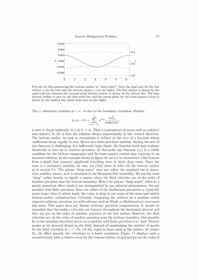
Figure 10. Reconstructing the bottom surface in “deep water”. Note the dual axes for the freesurface η (on the left) and the bottom surface ζ (on the right). The free surface is shown by thesolid bold line whereas the reconstructed bottom surface is shown by the dotted line. The truebottom surface is give by the thin solid line and the initial guess for the least-squares solver isshown by the dashed line (both with axes on the right).

The z−derivative vanishes at z = −h due to the boundary condition. Further,

φx(x,−h) =

∞∑n=−∞

einxinf̂n

cosh(nh),

is seen to decay uniformly in x as h→∞. Thus a consequence of terms such as cosh(kz)and sinh(kz) in (3) is that the solution decays exponentially in the vertical direction.The bottom surface we seek to reconstruct is defined as the zero of a function whosecoefficients decay rapidly to zero. Hence on a finite-precision machine, finding the zero ofthis function is challenging. For sufficiently large depth, the function itself may evaluateidentically to zero up to machine precision. At this point any function ζ(x) is a viablecandidate for the bottom topography and the least-squares routine may converge to anincorrect solution. In the example shown in figure 10, we try to reconstruct a flat bottomfrom a small (but nonzero) amplitude travelling wave in fairly deep water. Since thewave is a stationary solution, we may use (12a) alone to solve for the bottom surfaceas in section 3.1. The phrase “deep water” does not reflect the standard use in water-wave stability theory, as it is unrelated to the Benjamin-Feir instability. We use the word“deep” rather loosely to signify a regime where the fluid velocities are of the order ofmachine precision near the bottom boundary. Hence the phrase “deep water” refers to apurely numerical effect which is not distinguished by any physical phenomenon. On anymachine with finite precision, there are values of the shallowness parameter µ (typicallymuch larger than 1) which imply the water is deep in our sense of the term and inhibitbottom-surface reconstruction. Certainly, computing the solution on a machine whichsupports arbitrary precision (or with software such as Maple or Mathematica) overcomesthis issue. This paper does not discuss arbitrary precision computations. It should beremarked that the surface velocities are nonzero throughout the horizontal interval andthey are not on the order of machine precision at the free surface. However, the fluidvelocities are on the order of machine precision near the bottom boundary. One possiblefix to the situation described above on a machine with finite precision is to “lose” Fouriermodes as we proceed deeper in the fluid. Instead of maintaining the number of modesfor the fluid velocities at z = −h0 (15-16), equal to those used at the surface, we reduceKφ (in effect smooth the velocities) to a lower resolution. Figure 11 displays such areconstruction with a relative error for the bottom surface reconstruction on the order of


0 1 2 3 4 5 6

0.002

0.001

0.000

0.001

0.002

0.003

η

1.0

0.8

0.6

ζ

Figure 11. Reconstruction of the bottom surface in Section 4.2 using a lower resolution atz = −h0 than that of figure 10.

0 5 10 15 20 250.6

0.5

0.4

0.3

0.2

0.1

0.0

0.6

0.5

0.4

0.3

0.2

0.1

0.0

(a)

2 4 6 8 10 12 14 16

10-15

10-12

10-9

10-6

10-3

100

103

106

109

1012

(b)

Figure 12. Reconstruction of the sandbar profile (5) in deep water. Figure 12a compares the true(thin solid) and computed (dots) bottom surfaces. Figure 12b is a mode-by-mode comparison ofthe amplitude in Fourier space of the true (solid line) and computed solution (dots). The dashedline indicates the relative error in the amplitude of each mode.

10−11. Thus, for deeper water (µ large) we can reconstruct only the large-scale featuresof the bottom topography, effectively recovering the features corresponding to shallowwater. Of course, for sufficiently deep water, bathymetry reconstruction is practicallyimpossible.

The effect of deep water remains when considering non-stationary flow as is seen byconsidering the same bottom shape as given by equation (5) but at a deeper level. Figure12 depicts this situation for a reduced value of Kφ (about half of Kη). The relative errorin the reconstruction is O(10−2) for both the 2-norm and the infinity norm. In this case,the situation is further compounded by the fact that the nonlinear function is harderto evaluate due to the loss of precision as the argument of the hyperbolic functionsincreases. Indeed, the nonlinear function and its derivative do not obey relationship (1)for this example.

4.3. Localized free-surfaces

It is intuitively obvious that still water (no surface deviation and zero surface velocities)can be bounded by any bottom surface. The difficulty in proving uniqueness of solutionsto the set of equations (12a-12b) is in part due to this fact. Although the expressions aresimpler when the surface deviation is zero, uniqueness of solutions does not hold. In this


section we show this explicitly. Also we provide examples from simulations where thisbehaviour can be observed.

Given the nature of water-wave motion, if the surface deviation is nonzero, then thenormal velocity ηt at the surface must be nonzero as well. The method of reconstructionpresented in this manuscript requires (η, ηt, ηtt) 6= (0, 0, 0). In the case when (η, ηt, ηtt) =(0, 0, 0) the expressions for the nonlinear equations simplify considerably. They become

−i∑kn∈Λ

eiknx sinh(knζ)q̂x − ζx∑kn∈Λ

eiknx cosh(knζ)q̂x = 0, (2)

−i∑kn∈Λ

eiknx sinh(knζ)q̂xqxx − ζx∑kn∈Λ

eiknx cosh(knζ)q̂xqxx = 0, (3)

where we use Λ to indicate the one-dimensional version of the dual lattice described inSection 2. The periodicity of the function q implies these expressions can be rewritten as

∂x∑kn∈Λ

ieiknx sinh(knζ)q̂ = 0, (4)

∂x∑kn∈Λ

ieiknx sinh(knζ)q̂2x

2= 0. (5)

These equations possess infinitely many non-trivial solutions as any ζ satisfies theseequations for q constant since∫ L

0

eiknxCdx = C

∫ L

0

eiknxdx,

= Cδkn0,

where δkn0 is the Kronecker delta

δkn0 =

{1, kn = 0,0, kn 6= 0.

Following Craig et al. (2005), equation (4) is a reformulation of the boundary-valueproblem

φxx + φzz = 0, 0 < x < L, ζ < z < 0, (6a)

φz = 0, z = 0, (6b)

φz − ζxφx = 0, z = ζ. (6c)

The solution of this boundary-value problem may be written as

φ =

∞∑k=−∞

eikx cosh(kz)Φ̂k.

The boundary condition at z = ζ may be written in the form (4) with Φ̂ in the place ofq̂. In other words, q is the Dirichlet value at the surface z = 0 for the boundary-valueproblem associated with the first equation (2). The second equation (3) correspondsto a boundary-value problem with q2

x/2 as the Dirichlet value at the surface z = 0.Further, nontrivial q that solve (2) imply nontrivial solutions for the above BVP (6a-6c).However, since the only nontrivial solutions for φ in the above boundary-value problemare constants, q is at most a constant in (2) and q2

x/2 is at most a constant in (3).Hence q = C for some constant C. It should be noted that ζ can be any continuouslydifferentiable periodic function.


0 2 4 6 8 10 12

0.20

0.15

0.10

0.05

0.00

0.05

(a) True (thin solid line) and computed (dots)bottom surface.

0 2 4 6 8 10 120.04

0.03

0.02

0.01

0.00

0.01

0.02

0.03

0.04

(b) True and computed tangential velocity atsurface.

0 2 4 6 8 10 12

0.20

0.15

0.10

0.05

0.00

0.05

(c) True (thin solid line) and computed (dots)bottom surface.

0 2 4 6 8 10 120.04

0.03

0.02

0.01

0.00

0.01

0.02

0.03

0.04

(d) True and computed tangential velocity atsurface.

0 2 4 6 8 10 12

0.20

0.15

0.10

0.05

0.00

0.05

(e) True (thin solid line) and computed (dots)bottom surface.

0 2 4 6 8 10 120.04

0.03

0.02

0.01

0.00

0.01

0.02

0.03

0.04

(f) True and computed tangential velocity atsurface.

Figure 13. Recovering the bottom surface using localized surface deviations. Each row presentsa reconstruction based on a different localized surface elevation profile (bold solid line in theleft column). The left column shows true and computed bottom surfaces and the right columndepicts the computed tangential velocity at the surface.

As a consequence of the arguments presented above, we do not expect the least-squaresroutine to capture the true bottom surface when (η, ηt, ηtt) = (0, 0, 0). In practice, theleast-squares routine performs poorly when η is close to a constant and (ηt, ηtt) arenear machine epsilon. Consider the example depicted in figure 13 where we attemptto reconstruct the bottom surface using a localized free surface. Figure 13 shows three


different positions of the localized surface deviation. The left column displays the freesurface (bold solid line), reconstructed bottom surface (dashed line with dots) and truebottom surface (thin solid line). The right column compares the computed tangentialvelocity (dots) with the true tangential velocity (solid line). Of course, the localized freesurface implies velocities (and consequently ηt and ηtt) are negligible far away from thelocalized disturbance. Clearly, the recovery is much better at those locations where thefree-surface deviation is not negligible and poorer further away. It should be noted thatthe tangential velocity at the free surface is well resolved.

5. Examples revisited

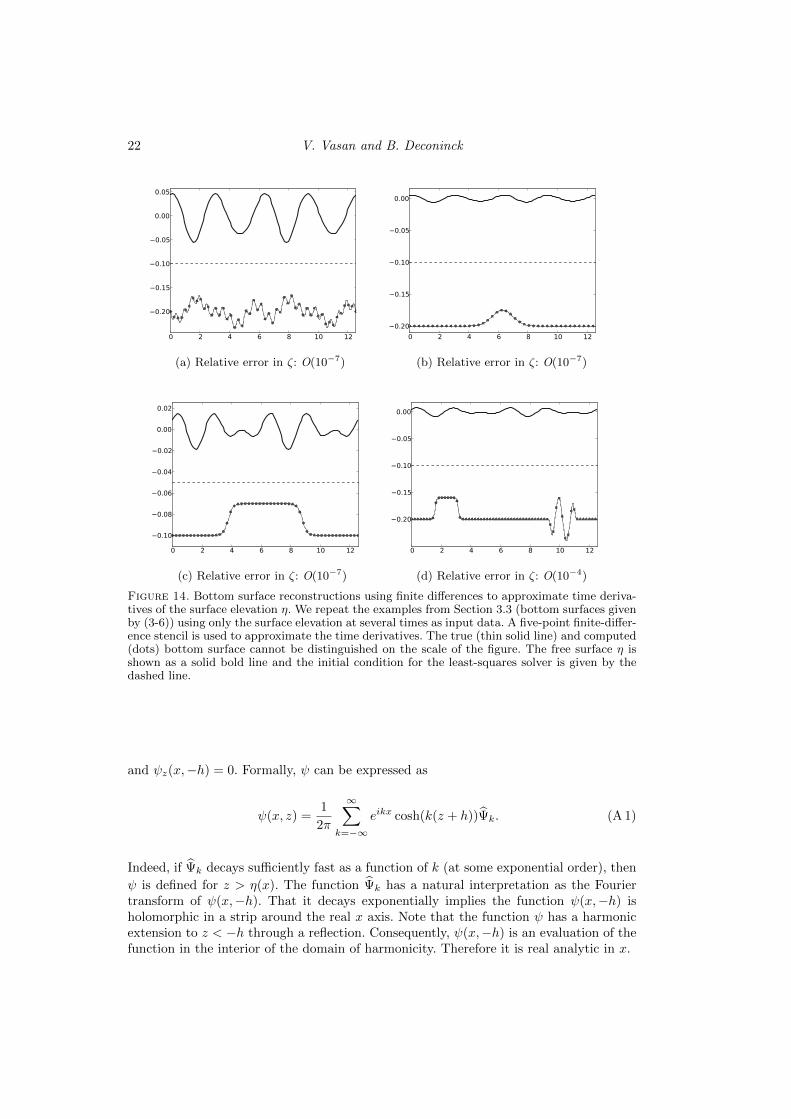
To finish, we present results for bottom surface recovery using the surface deviationη (but not its t−derivative) as a function of the horizontal variable x at several times.A five-point finite-difference stencil is used to compute the time derivatives ηt and ηtt.Figure 14 shows the bottom surface recovered for the examples of Section 3.3. All errorsreported are in the L2-norm. In all cases, relation (1) holds for the given input data andchoice of the parameters Kη and Kφ.

As seen in figure 14, the error induced by the finite-difference approximation of ηtand ηtt does not significantly affect the bathymetry reconstruction. The relative error inbottom surface reconstruction is certainly greater than that observed earlier in Section3.3 but not by much. As the reconstructions obtained using finite differences to computetime derivatives are remarkably accurate, we do not pursue more sophisticated methodsto compute t−derivatives. Further, the finite-difference stencil uses the surface elevationη at five points in time and thus requires minimal input data.

To conclude, we have presented a technique to reconstruct the bottom boundary ofan ideal incompressible irrotational fluid using only measurements of the free-surfaceelevation at several instances of time. The method makes no assumption on the magnitudeor form of the surface elevation. It is valid for both one- and two-dimensional surfaceprofiles and is, as expected, more accurate in the shallow-water regime than in deeperwater.

Appendix A. Weak formulation of Laplace’s Equation and theDirichlet→Neumann operator

Consider Laplace’s Equation

φxx + φzz = 0,

posed on the domain D = {(x, z) ∈ R2 : 0 < x < 2π,−h < z < η(x)}, where η is acontinuous periodic function with period 2π. Further assume that φ is periodic in thehorizontal variable x with period 2π, and

φz(x,−h) = 0, z = −h.

Let D(x) and N (x) be the Dirichlet and Neumann values of the function φ at z = η(x).If either D(x) or N (x) is provided to us, the problem is well posed in the Hadamardsense for D(x), N (x) in appropriate function spaces (Evans 1998).

Following Ablowitz & Haut (2008), consider a smooth function ψ which also satisfiesLaplace’s equation in D and the boundary condition at z = −h. Thus

ψxx + ψzz = 0, in D,


0 2 4 6 8 10 12

0.20

0.15

0.10

0.05

0.00

0.05

(a) Relative error in ζ: O(10−7)

0 2 4 6 8 10 12

0.20

0.15

0.10

0.05

0.00

(b) Relative error in ζ: O(10−7)

0 2 4 6 8 10 12

0.10

0.08

0.06

0.04

0.02

0.00

0.02

(c) Relative error in ζ: O(10−7)

0 2 4 6 8 10 12

0.20

0.15

0.10

0.05

0.00

(d) Relative error in ζ: O(10−4)

Figure 14. Bottom surface reconstructions using finite differences to approximate time deriva-tives of the surface elevation η. We repeat the examples from Section 3.3 (bottom surfaces givenby (3-6)) using only the surface elevation at several times as input data. A five-point finite-differ-ence stencil is used to approximate the time derivatives. The true (thin solid line) and computed(dots) bottom surface cannot be distinguished on the scale of the figure. The free surface η isshown as a solid bold line and the initial condition for the least-squares solver is given by thedashed line.

and ψz(x,−h) = 0. Formally, ψ can be expressed as

ψ(x, z) =1

2π

∞∑k=−∞

eikx cosh(k(z + h))Ψ̂k. (A 1)

Indeed, if Ψ̂k decays sufficiently fast as a function of k (at some exponential order), then

ψ is defined for z > η(x). The function Ψ̂k has a natural interpretation as the Fouriertransform of ψ(x,−h). That it decays exponentially implies the function ψ(x,−h) isholomorphic in a strip around the real x axis. Note that the function ψ has a harmonicextension to z < −h through a reflection. Consequently, ψ(x,−h) is an evaluation of thefunction in the interior of the domain of harmonicity. Therefore it is real analytic in x.


Using Green’s Identity, we have

0 =

∫D

(ψ(φxx + φzz)− φ(ψxx + ψzz)) dxdz,

=

∫∂D

(ψ∂φ

∂n− φ∂ψ

∂n

)dS,

=

∫ 2π

0

ψ(x, η) [φz(x, η)− ηxφx(x, η)] dx−∫ 2π

0

φ(x, η) [ψz(x, η)− ηxψx(x, η)] dx,

=

∫ 2π

0

ψ(x, η)N (x)dx−∫ 2π

0

D(x) [ψz(x, η)− ηxψx(x, η)] dx, (A 2)

where ∂/∂n is the normal derivative to the surface. Hence φ may be regarded as a weaksolution to Laplace’s Equation. Using the representation (A 1) for ψ and noting that

eikx (ik sinh(k(η + h)) + kηx cosh(k(η + h))) = ∂x(eikx sinh(k(η + h))

),

we obtain after an integration by parts

∞∑k=−∞

Ψ̂k

(∫ 2π

0

eikx [cosh(k(η + h))N (x)− i sinh(k(η + h))D ′(x)] dx

)= 0. (A 3)

Since this relation is valid for arbitrary Ψ̂k, we obtain the usual global relation forLaplace’s Equation derived by Ablowitz et al. (2006) (hereafter known as the AFMglobal relation). In light of this derivation, we arrive at an alternative interpretation: theglobal relation holds as a distribution. Indeed expressions such as∫ 2π

0

eikx cosh(k(η + h))N (x)dx,

∫ 2π

0

eikx sinh(k(η + h))D ′(x)dx,

define a functional over a suitable space of functions, namely those that decay at leastlike e−M |k| where M = max(|η + h|) as is easily seen by applying the Cauchy-Schwarzinequality. As noted in Ablowitz & Haut (2008), the expressions above are themselveslinear operators that map the Dirichlet and Neumann values on the boundary to distri-butions. The authors take an inverse Fourier transform of the AFM global relation toobtain a dual formulation for the water-wave problem. The Fourier transform is definedthrough duality using the inner-product (A 3), as the distributions we are consideringare certainly not classical ones.

However, a more straightforward approach to the dual formulation is as follows. Equa-tion (A 3) is written as∫ 2π

0

N (x)

( ∞∑k=−∞

Ψ̂keikx cosh(k(η + h))

)dx

+ i

∫ 2π

0

D(x)∂x

( ∞∑k=−∞

Ψ̂keikx sinh(k(η + h))

)dx = 0. (A 4)

The above relation is an equality between two inner products. Since the Dirichlet problemfor the Laplace Equation is well posed for all suitable D(x), the above equation implies

∞∑k=−∞

Ψ̂keikx cosh(k(η + h)) = D(x), (A 5)


and

−i∂x

( ∞∑k=−∞

Ψ̂keikx sinh(k(η + h))

)= N (x). (A 6)

This is equivalent to choosing of ψ = φ in (A 2). Note that the normal derivative to(A 1) is indeed given by the expression (A 6). The above pair of equations defines the

Dirichlet→Neumann operator in terms of the parameter Ψ̂k. This same pair appears inAblowitz & Haut (2008) in the dual formulation of the water-wave problem. The Fouriertransform of (A 5-A 6) leads to

∞∑k=−∞

Ψ̂kAkl = D̂l,

∞∑k=−∞

Ψ̂kBkl = N̂l,

with

Akl =

∫ 2π

0

eikx−ilx cosh(k(η + h))dx, Bkl = l

∫ 2π

0

eikx−ilx sinh(k(η + h))dx.

As noted by Craig et al. (2005), the operator Akl is invertible. Equations (A 5-A 6) definethe Dirichlet→Neumann operator. It should be noted that this is not a perturbative orsmall amplitude in η representation for the Dirichlet→Neumann operator. Indeed, weare able to simulate large amplitude water waves using this form of the operator (seeAppendix B).

The associated problem with a variable topography may be addressed similarly. At thebottom topography, we have the Neumann condition

∂φ

∂n(x,−h−H(x)) = 0,

where H is a continuously differentiable periodic function of x with period 2π. We startwith Green’s Identity as before to obtain the appropriate generalization of the formulation(A 5-A 6) to varying topography. Alternately, we may start with the following globalrelations, see Ablowitz et al. (2006):∫ 2π

0

eikx (cosh(k(η + h))N (x)− i sinh(k(η + h))D ′(x)− i sinh(kH)Φx) dx = 0, (A 7)∫ 2π

0

eikx (i sinh(k(η + h))N (x) + cosh(k(η + h))D ′(x)− cosh(kH)Φx) dx = 0, (A 8)

where Φ(x) = φ(x,−h−H). Taking the inner product of the first equation with Ψ̂1k, the

second with Ψ̂2k and adding the resulting equations, we obtain after an integration by

parts ∫ 2π

0

∞∑k=−∞

eikx(

Ψ̂1k cosh(k(η + h)) + iΨ̂2

k sinh(k(η + h)))

N (x)dx

+

∫ 2π

0

∂x

∞∑k=−∞

eikx(iΨ̂1

k sinh(k(η + h))− Ψ̂2k cosh(k(η + h))

)D(x)dx

+

∫ 2π

0

∂x

∞∑k=−∞

eikx(iΨ̂1

k sinh(kH) + Ψ̂2k cosh(kH)

)Φ = 0.


The above equation can be obtained from Green’s Identity (A 2) with the choice

ψ =

∞∑k=−∞

eikx(

Ψ̂1k cosh(k(z + h)) + iΨ̂2

k sinh(k(z + h))).

Imposing suitable boundary conditions, we obtain the following system of equations forΨ̂1k and Ψ̂2

k

∞∑k=−∞

eikx(


k sinh(k(η + h)))

= D(x), (A 9)

∂x

∞∑k=−∞

eikx(iΨ̂1

k sinh(kH) + Ψ̂2k cosh(kH)

)= 0. (A 10)

On taking the Fourier transform of these equations, we arrive at a linear system ofequations for Ψ̂1

k and Ψ̂2k. Finally the Neumann condition at the surface z = η is given

by

N (x) = −i∂x∞∑

k=−∞

eikx(

Ψ̂1k sinh(k(η + h)) + iΨ̂2

k cosh(k(η + h))).

Remark A.1. A similar calculation is valid for the infinite-line case.

Appendix B. The forward problem: simulating the dynamics of thewater-wave equations in a periodic domain

Euler’s Equations for one-dimensional surface water-waves are given by

φxx + φzz = 0, 0 < x < 2π, ζ < z < η,

φz − ζxφx = 0, z = ζ(x),

φz − ηxφx = ηt, z = η(x, t),

φt +1

2φ2x +

1

2φ2z + η = 0, z = η(x, t).

To numerically integrate these equations in time, we rewrite the above equations as“evolution equations” for η and q = φ(x, η, t):

ηt = G(η, ζ)q,

qt = −gη − 1

2[H1(η, ζ)q]2 − 1

2[H2(η, ζ)q]2 + ηtH2(η, ζ)q,

where G is the usual Dirichlet→Neumann operator for the Laplace equations. Analo-gously, the operator H1 maps the Dirichlet data at the surface z = η to the horizontalderivative φx at the surface z = η, and H2 takes the Dirichlet data to the vertical deriva-


t

11.2

0.00

0.00

x

6.28

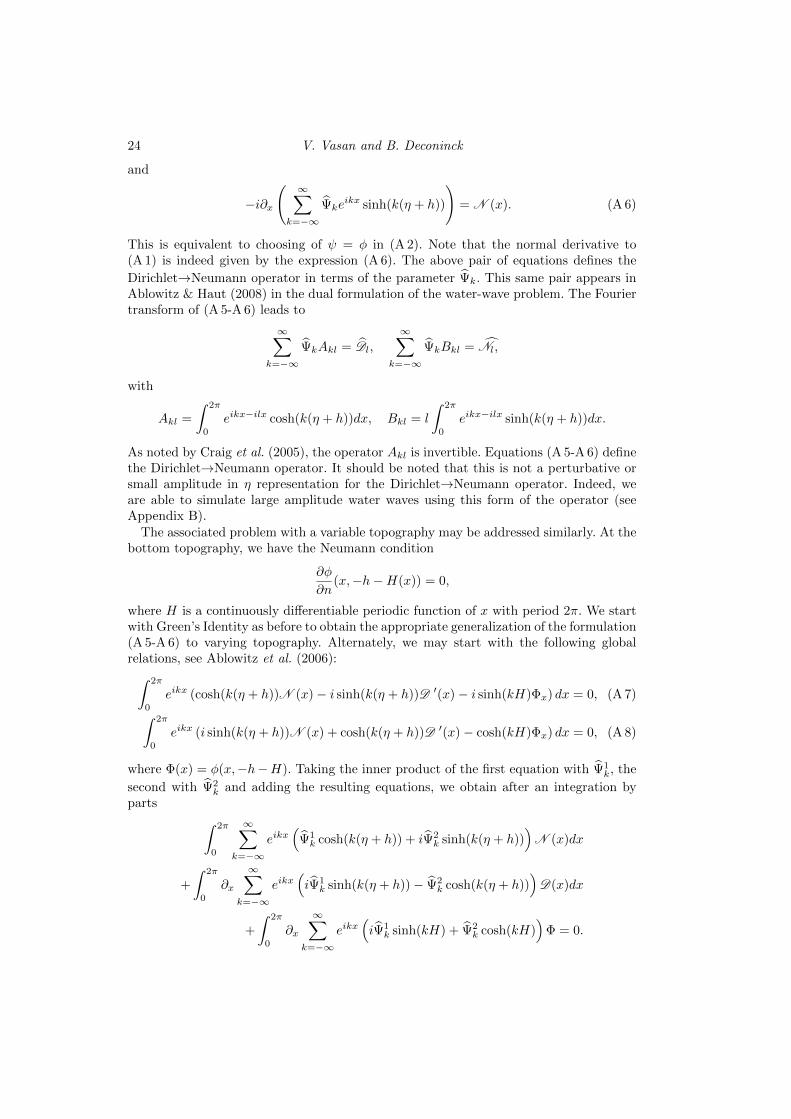
Figure 15. Evolution of an unsteady wave.

tive φz at the surface z = η. These operators are computed using the following formulae:

G(η, ζ)q = −i∂x∞∑

k=−∞

eikx(


k cosh(k(η + h))),

H1(η, ζ)q =

∞∑k=−∞

ikeikx(


k sinh(k(η + h))),

H2(η, ζ)q =

∞∑k=−∞

keikx(


k cosh(k(η + h))).

Here Ψ̂1k and Ψ̂2

k satisfy (A 9-A 10). The evolution equations for η and q are integratedin time using the Fourth-Order Runge-Kutta Method with spectral approximation offunctions in the x variable. Numerical simulations are fully de-aliased using zero padding.In practice, de-aliasing the nonlinearities assuming they are at most cubic is sufficient.

We present two example simulations using the method described above. The exam-ples are similar to those of Craig & Sulem (1993). Our goal is not to present detailedcomputations, rather it is to establish that the numerical method introduced in this sec-tion produces satisfactory results. More details and extensive examples on the numericalsolution of the Euler Equations for the time-dependent motion of the surface will bepresented in a future paper. The first example is a simulation of unsteady flow. For thesecond example we use an approximate Stokes wave as the initial condition.

B.1. Unsteady flow

Our first simulation is to compute the evolution of the free surface with initial condition

η0(x) = 0.01e−4(x−π)2 cos(4x),

with zero initial velocity potential. The spatial period of the flow is 2π. Figure 15 showsthe evolution of the surface up to t = 11.25. The simulation is stable and can be continuedlonger. The computation was performed with 64 collocation points and full de-aliasingwas accomplished using zero padding. Figure 16 depicts the time series for the relativeerror in the Hamiltonian and the absolute error in the momentum. Evidently, thesequantities are conserved well for the duration of the simulation.


0 2 4 6 8 10

10-22

10-20

10-18

10-16

10-14

Figure 16. Time series of the Hamiltonian and the momentum for an unsteady wave. Relativeerror in the Hamiltonian is shown by the solid line and the absolute error in the momentum isshown by the dashed line.

B.2. An approximate Stokes wave

Our second simulation uses the following second-order approximation to a Stokes waveas the initial condition:

η0(x) = a cos(kx) + µ2a2 cos(2kx),

q0(x) = ν1a cosh(k(η0 + h)) sin(kx) + ν2a2 cosh(2k(η0 + h)) sin(2kx),

with

µ2 =1

2k coth(kh)

(1 +

3

2 sinh2(kh)

),

ν1 =ω

k sinh(kh), ν2 =

3

8

ω

sinh4(kh),

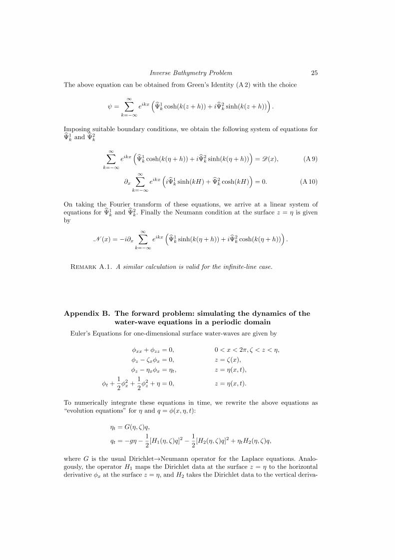
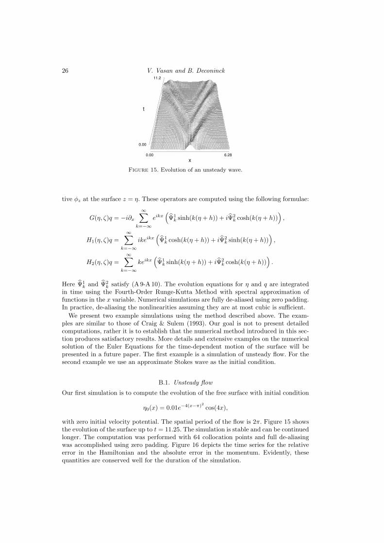
where ω2 = k tanh(kh). Figure 17 displays the evolution of a 2π-periodic wave with k = 2,a = 0.065 and h = 1. The wave is near the linear regime and the Stokes expansion aboveis seen to be a fairly accurate representation of the full wave. We show in figure 17 thewave translating over two full periods. The calculation is carried out further in time withalmost no change in the profile. Since the initial condition is only an approximation to aStokes wave, the peaks of the wave profile show small oscillations as the wave translates.Again the Hamiltonian and momentum are conserved (figure 18).

REFERENCES

Ablowitz, M. J., Fokas, A. S. & Musslimani, Z. H. 2006 On a new non-local formulationof water waves. J. Fluid Mech. 562, 313–343.

Ablowitz, M. J. & Haut, T. S. 2008 Spectral formulation of the two fluid Euler equationswith a free interface and long wave reductions. Analysis and Applications 6, 323–348.

Collins, M. D. & Kuperman, W. A. 1994 Inverse problems in ocean acoustics. Inverse Prob-lems 10, 1023–1040.

Craig, W., Guyenne, P., Nicholls, D. P. & Sulem, C. 2005 Hamiltonian long-wave expan-sions for water waves over a rough bottom. Proc. R. Soc. A 461, 839–873.

Craig, W. & Sulem, C. 1993 Numerical simulation of gravity waves. J. Comp. Phys. 108,73–83.

Deconinck, B. & Oliveras, K. 2011 The instability of periodic surface gravity waves. J. FluidMech. 675, 141–167.

Evans, L. 1998 Partial Differential Equations. Providence, RI,: American Mathematical Society.


t

6.20

0.00

0.00

x6.28

Figure 17. Evolution of an approximate Stokes wave.

0 1 2 3 4 5 610-17

10-16

10-15

10-14

10-13

Figure 18. Time series of the Hamiltonian and the momentum for an approximate Stokes wave.Relative error in the Hamiltonian is shown as a solid line, relative error in the momentum isshown by the dashed line.

Grilli, S 1998 Depth inversion in shallow water based on nonlinear properties of shoalingperiodic waves. Coastal Engineering 35, 185209.

Guenther, R. B. & Lee, J. W. 1996 Partial differential equations of mathematical physicsand integral equations. Mineola, NY: Dover Publications Inc.

Lannes, D. 2005 Well-posedness of the water-wave equations. J. Amer. Math. Soc. 18, 605–654.Nicholls, D. P. & Taber, M. 2008 Joint analyticity and analytic continuation of Dirichlet-

Neumann operators on doubly perturbed domains. J. Math. Fluid Mech. 10, 238–271.Paley, R. C. & Wiener, N. 1934 Fourier transforms in the complex domain, Colloquium

Publications, vol. 19. Providence, RI: American Mathematical Society.Piotrowski, C. & Dugan, J. 2002 Accuracy of bathymetry and current retrievals from air-

borne optical time-series imaging of shoaling waves. IEEE Trans. on Geoscience and RemoteSensing 40, 2606–2618.

Taroudakis, M. I. & Makrakis, G. 2001 Inverse Problems in Underwater Acoustics. Springer-Verlag, New York.

Wu, S. 2011 Global wellposedness of the 3-D full water wave problem. Invent. Math. 184,125–220.

Zakharov, V. E. 1968 Stability of periodic waves of finite amplitude on the surface of a deepfluid. Zhurnal Prikladnoi Mekhaniki i Tekhnicheskoi Fiziki 8, 86–94.

Date post:	01-Dec-2021
Category:	Documents
Upload:	others
View:	2 times
Download:	0 times

The inverse water wave problem of bathymetry detection

Documents