Page 1
1
The investment perspective of accruals: Do theories of investment under uncertainty
provide insight into the factors that shape a firm’s level of accruals?
Salman Arif
Indiana University
[email protected]
Nathan Marshall
Indiana University
[email protected]
Teri Lombardi Yohn*
Indiana University
[email protected]
1309 E 10th
Street
Kelley School of Business
Indiana University
Bloomington, IN 47405
(812) 855-8966
April 2014
* Corresponding author
We would like to thank Eric Allen, Daniel Beneish, Frank Ecker, Patricia Fairfield, Richard
Frankel, Paul Hribar, Chad Larson, Andy Leone, Gerald Lobo, Andrey Malenko, DJ Nanda, Lee
Pinkowitz, Paul Pronobis, Scott Richardson, Amy Sun, Lakshmanan Shivakumar, Mark Soliman,
Irem Tuna, Peter Wysocki and seminar participants at London Business School, University of
Southern California, University of Houston, University of Miami, Georgetown University, the
Conference on Financial Economics and Accounting, and the Midwest Accounting Conference
for their comments and suggestions.
Page 2
2
The investment perspective of accruals: Do theories of investment under uncertainty
provide insight into the factors that shape a firm’s level of accruals?
Abstract
Accounting research has long relied on accruals-based measures of earnings management.
However, there is little understanding of the economic forces that shape a firm’s accruals over
time. We consider accruals in their role as a form of investment and examine whether theories of
investment under uncertainty shed light on whether accruals are affected by changes in the
business environment over time. Specifically, theories of investment under uncertainty posit that
higher uncertainty leads firms to withhold investment, leading to a negative relation between
investment and uncertainty. Consistent with the theory, we document a significant negative
relation between working capital accruals and uncertainty. Furthermore, we find that the negative
relation between accruals and uncertainty is more pronounced for firms with longer operating
cycles. The sensitivity of specific accruals to uncertainty also strengthens as the horizon of the
accrual increases. Lastly, we document a robust negative relation between abnormal accruals and
uncertainty, which strengthens as the operating cycle increases. These results suggest that
abnormal accruals are systematically associated with the level of uncertainty faced by the firm
and that researchers should consider the effect of uncertainty, the components of accruals, and
the firm’s operating cycle when relying on abnormal accrual models to capture earnings
management.
Page 3
1
The investment perspective of accruals: Do theories of investment under uncertainty
provide insight into the factors that shape a firm’s level of accruals?
1. Introduction
A vast body of accounting research relies on accruals-based measures of earnings
management. This literature distinguishes ‘normal’, or ‘expected’ accruals from ‘abnormal’, or
‘discretionary’ accruals by directly modeling the accrual generating process. However, there is
little theoretical understanding of the fundamental economic forces that shape the level of a
firm’s expected accruals (e.g. Dechow et al (2010), Defond (2010)). Moreover, commonly
employed abnormal accrual models tend to be estimated in the cross-section, despite the fact that
the accrual generating process is likely to be dynamic. Indeed, recent research highlights that
little is known empirically and theoretically about the time-varying process that characterizes
accruals (Owens, Wu and Zimmerman (2013); Gerakos (2012)).
In this paper, we employ the rich theoretical framework of investment under uncertainty
found in the economics literature to study whether the theory can explain intertemporal variation
in the level of a firm’s accruals. Additionally, we exploit the theory to study when the impact of
uncertainty on accruals is particularly pronounced. Prior research on accruals notes that accruals
can be viewed as a component of investment. Thus, accruals at least partially reflect a deliberate
investment choice by the firm (Fairfield et. al., 2003; Zhang, 2007; Wu et al., 2010; Bushman et.
al., 2011; Allen et al., 2013; Momentè et al., 2013). Adopting this perspective of accruals
suggests that economic theories of investment may provide insight into the behavior of accruals.
As such, we note at the very outset that our study is a joint test of the extent to which accruals
reflect investment decisions and the extent to which theories of investment under uncertainty
provide insight into accrual behavior.
Page 4
2
In investment under uncertainty theory, time-varying uncertainty plays a critical role in
investment decisions because firms cannot perfectly forecast the future. Firms must therefore
make investment decisions in the face of uncertainty, and uncertainty enters as a key variable in
investment decision making (e.g., Bernanke, 1983; McDonald and Siegel, 1986; Ingersoll and
Ross, 1992; Dixit and Pindyck, 1994; Schwartz and Trigeorgis, 2004; Grenadier and Malenko,
2010).
Using a real options approach, the theory suggests that the investment-uncertainty
relation is negative. The underlying intuition is that when firms make investment decisions under
uncertainty, they trade off the returns earned from investing today against the benefit from
delaying investment to the future, when information or business conditions may be better. The
benefit of postponing investment – known as the “option to wait” – implies that when
uncertainty rises, the value of the option to wait is higher. Higher uncertainty thereby has a
dampening effect on investment as firms prefer to “wait and see” instead of investing
immediately. Thus, the theory predicts a negative relation between investment and uncertainty.
Accordingly, our first set of tests focuses on testing the relation between net working capital
accruals and uncertainty.
At a broad level, we recognize that accounting accruals are shaped by a multitude of
forces besides managers’ investment decisions. First, accruals may be subject to intentional
manipulation by managers (Dechow et al, 2010) and/or unintentional mismeasurement
(Richardson et al 2005). Second, accruals are used to resolve the timing and matching issues
related to cash flows as a performance metric (Dechow 1994), and are therefore shaped by the
accounting standards that pertain to each specific accrual (Healy and Wahlen 1999). Third,
accruals may be affected by parties outside of the firm, including customers (through accounts
Page 5
3
receivables) and suppliers (through accounts payables).1 Therefore, even if accruals are partially
shaped by investment decisions, the simultaneous actions of these diverse forces may obscure
any relation between uncertainty and accruals as asserted by investment under uncertainty
theory.
To empirically test our predictions, we examine the relation between working capital
accruals and uncertainty for firms with available annual data from 1965 through 2010. We
examine three measures of uncertainty; namely, total volatility of stock returns, industry
volatility of stock returns, and analyst forecast dispersion. These measures of uncertainty are
consistent with those used in the prior literature to capture uncertainty about the firm’s future
prospects (e.g. Ang et. al., 2006; Eisdorfer, 2008; Diether et. al., 2002). Additionally, the use of
industry-level volatility alleviates concern that our results are driven by reverse causality. Based
on prior literature addressing corporate investment decisions (Hayashi, 1982; Lamont, 1997;
Eisdorfer, 2008), our regression model includes controls for the firm’s prior and current cash
flows, prior and current stock returns, book-to-market, size, and leverage. In addition, since the
economic theory relates to explaining the level of accruals within a firm over time, we include
firm fixed effects in all our regressions. This has the added benefit of removing firm-level
correlated omitted variables that are invariant over the sample period.
Our first key result is that there is a robust negative relation between net working capital
accruals and uncertainty. This result is consistent with the economic theory, and suggests that
1 We note that because net working capital accruals are equal to current asset accruals net of current liability
accruals, it is not clear that the relation between net working capital accruals and uncertainty will be negative. For
example, if the firm’s creditors are less (more) willing to extend credit to the firm when uncertainty rises (declines),
then accounts payables and other current liabilities will be negatively associated with uncertainty. This would
contribute positively to the association between net working capital accruals and uncertainty. Therefore, the overall
relation between net working capital accruals and uncertainty may be positive if the sensitivity of current liability
accruals to uncertainty is reliably more negative compared to the sensitivity of current assets accruals to uncertainty.
Page 6
4
managers withhold investment in working capital accruals when uncertainty rises. We next
decompose net working capital accruals into its constituent accrual components to further
investigate which accruals drive the overall negative relation. We find that inventory accruals
and accounts receivables have the strongest negative relation with uncertainty. This indicates that
when uncertainty rises, managers invest less in inventory and invest less in granting credit to
their customers.2 Interestingly, accounts payable is also negatively associated with uncertainty.
However, the negative coefficient on accounts payable is attenuated compared to the negative
coefficient on inventory and accounts receivable. In other words, when uncertainty rises, the
lower net investment in working capital arises because the lower investments in inventory and
accounts receivables are only partially offset by lower accounts payables.
We next exploit the theory’s real options framework to form predictions on the types of
firms where uncertainty has the largest impact on accruals. The operating cycle measures the
average time between the disbursement of cash to produce a product and the receipt of cash from
the sale of the product (Dechow, 1994). Firms with longer operating cycles will have a wider
range of possible investment outcomes and greater exposure to changing business conditions.
This suggests that the option to wait is more valuable for firms with longer operating cycles.
Thus, under the hypothesized economic framework, we expect uncertainty to have a stronger
dampening effect on net investment in working capital for firms with a longer operating cycle.
We find evidence consistent with this conjecture. More specifically, we find that the working
capital accruals of firms in the longest quintile of operating cycle are at least twice as sensitive to
uncertainty compared to those of firms in the shortest quintile of operating cycle.
2 The fact that accounts receivable is negatively associated with uncertainty does not mean that firms are willing to
forgo sales when uncertainty rises. Untabulated tests show that the fraction of sales made on credit declines when
uncertainty rises, indicating that firms are less willing to invest in granting credit to customers, and that they make
more sales on cash, when uncertainty rises.
Page 7
5
We further exploit the theory to investigate when the effect of uncertainty is likely to be
more or less pronounced. Specifically, we study whether the sensitivity of individual accruals to
uncertainty is a function of the accrual’s horizon. We independently sort firms into quintiles
based on accounts receivable days, inventory days, and accounts payable days. We then calculate
the sensitivity of their accounts receivable accrual, inventory accrual, and accounts payable
accrual to uncertainty within each horizon quintile (respectively). Consistent with our
hypothesis, we find that the longer the horizon of the specific accrual, the more sensitive the
accrual is to uncertainty. In other words, the accounts receivables of firms in the longest quintile
of accounts receivable days are much more sensitive to uncertainty than the accounts receivables
of firms in the shortest quintile of accounts receivable days (similarly for inventory and accounts
payable).
Finally, we examine the relation between uncertainty and commonly employed measures
of both normal and abnormal accruals. If extant accrual models fail to purge fundamental
economic forces from abnormal accruals, then uncertainty may be systematically associated with
abnormal accruals. Moreover, given that economic theory suggests that the effect of uncertainty
is particularly pronounced for firms with a longer operating cycle, we expect the bias in
abnormal accruals to be exacerbated for firms with a longer operating cycle. On the other hand,
our empirical tests may lack power given that prior empirical accounting research suggests that
firms with longer operating cycles have greater absolute levels of earnings management (e.g.
Dechow and Dichev 2002).
Using six different abnormal accrual models found in prior work, we decompose net
working capital accruals into normal and abnormal components and test the relation with
uncertainty. Across all six models, we document a robust negative relation between normal
Page 8
6
accruals and uncertainty. Furthermore, we document a robust negative relation between
abnormal accruals and uncertainty across all six models. Lastly, we find that the abnormal
accruals of firms in the longest operating cycle quintile are at least twice as sensitive to
uncertainty compared to those of firms in the shortest quintile of operating cycle. Collectively,
these results suggest that extant abnormal accrual models fail to cleanly separate between
earnings management activities and the fundamental economic forces that shape accruals.
We contribute to the literature in several ways. First, understanding the properties of
accruals is among the chief goals of financial accounting research. Dechow et al (2010), Defond
(2010), Ball (2013) and others express concern that there is little theory to guide researchers in
understanding the factors that shape the level of a firm’s accruals. We draw on investment under
uncertainty theories and examine the extent to which these theories apply to the behavior of
accruals. To our knowledge, our study is the first to link accounting accruals to the investment
under uncertainty literature. Our empirical results provide important insight into accrual behavior
vis-à-vis the level of uncertainty faced by the firm. Consistent with economic theory, we
document a robust negative relation between accruals and uncertainty. Furthermore, we exploit
the theory to identify the types of firms where uncertainty has the largest impact on accruals. We
predict and find evidence that the effect of uncertainty on accruals is particularly pronounced in
firms with long operating cycles. Moreover, this holds true even for abnormal accruals.
Our findings provide valuable insights for researchers seeking to use abnormal accruals
as a proxy for earnings management (Healy, 1985; DeAngelo, 1986; Jones, 1991; Dechow et. al.,
1995; Dechow et. al., 2003). Our analyses show that abnormal accruals vary systematically with
the uncertainty faced by the firm. This contributes to recent research that attempts to identify and
correct for systematic biases in abnormal accrual models (e.g., Owens, Wu, and Zimmerman,
Page 9
7
2013), and suggests that researchers should potentially consider the role of uncertainty and
accrual horizon when calculating accruals-based proxies for earnings management. Lastly, we
believe that future research could perhaps combine the investment under uncertainty predictions
with other relevant economic theories to further identify systematic biases in abnormal accruals
models and to enhance models of expected accruals.
The paper proceeds as follows. Section 2 presents the background and hypothesis
development. Section 3 presents variable definitions and descriptive statistics. Section 4 presents
empirical results, and Section 5 concludes.
2. Background and hypotheses development
2.1. Prior literature on accruals
Accruals are fundamental to financial reporting and are the underlying innovation of
accounting. The accounting literature generally considers accruals from one of three
perspectives. Under the first perspective, accruals arise as a secondary outcome of the earnings
reporting process. For example, Dechow (1994) focuses on the role of accruals in mitigating the
timing problems associated with cash flows as a performance metric. The second perspective
views accruals as a component of profitability and highlights that the accrual component of
earnings involves greater subjectivity than the cash flow component. Based on this
characterization of accruals, the research asserts that at least some portion of accruals reflects
intentional and unintentional mismeasurement (Sloan, 1996; Xie, 2001). The third perspective
considers the role of accruals as a component of investment. Fairfield et. al. (2003) note that
growth in net operating assets can be disaggregated into accruals and growth in long-term net
operating assets. They note, therefore, that accruals are not only a component of profitability but
Page 10
8
also a component of investment. Zhang (2007) supports the investment role of accruals and
concludes that the accrual anomaly documented by Sloan (1996) is primarily attributable to the
role of accruals as a form of investment. Bushman et al. (2011) note that working capital accruals
reflect investment decisions and examine the implications of this for investment-cash flow
sensitivities.
While these views of accruals have been examined in the context of explaining the
differential persistence of accruals and operating cash flows and the market mispricing of
accruals (Dechow and Dichev, 2002; Fairfield et al., 2003; Zhang, 2007; Allen et al., 2013), little
research has exploited these perspectives to aid in understanding the factors that shape a firm’s
level of accruals. In this study, we rely on the investment perspective of accruals and examine
whether theories of investment under uncertainty provide insight into the relation between the
level of accruals and uncertainty. We note that our analyses, therefore, provide a joint test of the
extent to which accruals reflect investment and whether the finance theories of investment under
uncertainty apply to working capital accruals.3
2.2. Hypotheses development
Real-world investment decisions tend to share three features, which collectively motivate
theories of investment under uncertainty (Dixit, 1992). First, firms cannot perfectly forecast the
3 Prior research has examined the relation between the volatility and absolute value of discretionary accruals and
uncertainty. Ghosh and Olsen (2009) suggest that the absolute value of discretionary accruals rises with
environmental uncertainty. Chen et al. (2012) find that idiosyncratic return volatility rises with the volatility of
discretionary accruals. However, this prior work does not study the relation between uncertainty and the level of a
firm’s accruals.
Page 11
9
future because the business environment has ongoing uncertainty and information arrives
gradually. Second, investment is costly and difficult to reverse, i.e. investment tends to be
“irreversible”. Third, an investment opportunity does not generally disappear if no investment is
made immediately, i.e. firms generally have the option to postpone investment to the future.
Motivated by these observations, a large theoretical literature examines investment under
uncertainty and generally finds a negative relation between investment and uncertainty (e.g.
Bernanke, 1983; McDonald and Siegel, 1986; Ingersoll and Ross, 1992; Dixit and Pindyck,
1994; and Schwartz and Trigeorgis, 2004).
Relying on real options logic, the general intuition underlying theoretical models of
investment under uncertainty is as follows. A manager’s investment decision involves a tradeoff
between investing immediately or instead postponing investment to the future. The benefit of
immediate investment is that the firm is able to start enjoying returns from the investment. On
the other hand, the benefit of waiting is that the manager can gain more information about the
value of the investment and take advantage of any improvements in business conditions that
occur in the meantime. This benefit of waiting introduces an opportunity cost to investing today.
At the point when the benefits of waiting equal the costs of waiting, investment occurs.4 When
uncertainty is higher, the benefit of waiting (commonly referred to in the literature as the “option
to wait”) is higher. Firms therefore become more cautious in their investment behavior because
they prefer to “wait and see” what happens in the future. Thus, the models predict a negative
investment-uncertainty relation. Empirical research in finance generally supports the negative
relation between investment and uncertainty (e.g. Leahy and Whited, 1996; Guiso and Parigi,
4 This logic demonstrates that in the presence of uncertainty, investment decisions are not simply based on the
common net present value rule that suggests investment in a project when the net present value of the project is
positive. Instead, investment occurs if the net present value of the investment project exceeds the value of the option
to wait. Thus, incorporating uncertainty into the decision process leads to a more nuanced approach to investment.
Page 12
10
1999; Minton and Schrand, 1999; and Bond and Cummins, 2004). To the extent that accruals
reflect a component of investment, we expect working capital accruals (i.e., growth in working
capital) to be negatively associated with uncertainty.
We note, however, that it is not clear that we will find a negative relation between
accruals and uncertainty empirically given that accounting accruals are shaped by a multitude of
forces. Accruals may be subject to intentional or unintentional manipulation by managers
(Dechow et al, 2010; Richardson et al 2005). Accruals are also used to resolve the timing and
matching issues related to cash flows as a performance metric and are shaped by the accounting
standards that pertain to each specific accrual (Dechow 1994; Healy and Wahlen 1999). Accruals
may also be affected by parties such as customers and suppliers. Therefore, even if accruals are
partially shaped by investment decisions, the simultaneous actions of these other diverse forces
may obscure any relation between uncertainty and accruals as asserted by the investment under
uncertainty theory. Despite this caveat, we predict a negative relation between uncertainty and
accruals. This leads to our first hypothesis:
H1: The level of working capital accruals is negatively associated with the level of
uncertainty.
Our second hypothesis predicts an increasing relation between the sensitivity of accruals
to uncertainty and the length of the firm’s operating cycle. The operating cycle measures the
average time between the disbursement of cash to produce a product and the receipt of cash from
the sale of the product (Dechow, 1994). A firm with a longer operating cycle has greater
exposure to changing business conditions. More specifically, a longer operating cycle leads to a
wider range of possible investment outcomes, which makes the option to wait more valuable.
Thus, we expect that uncertainty has a stronger dampening effect on working capital accruals in
firms with longer operating cycles.
Page 13
11
There are, however, reasonable arguments to assert that the negative accrual-uncertainty
relation weakens for firms with longer operating cycles. Zang (2012) asserts that accruals-based
earnings management is a positive function of the opportunities and a negative function of the
costs associated with this form of earnings management. Zang (2012), therefore, suggests that
greater flexibility leads to more accrual-based earnings management, and consistent with this
notion, documents a positive relation between abnormal accruals and the length of the firm’s
operating cycle. Given that uncertainty and the length of the firm’s operating cycle lead to
greater flexibility and more opportunities for earnings management, these results suggest that the
negative accrual-uncertainty relation weakens for firms with longer operating cycles. Despite this
reasonable argument for the null hypothesis, we present our second hypothesis based on our
theoretical economic framework as follows:
H2: The negative association between the level of working capital accruals and
uncertainty is more pronounced for firms with longer operating cycles.
Finally, we predict that the relation between accruals and uncertainty leads to systematic
biases in abnormal accruals measures, which are widely used as a proxy for earnings
management. In capturing earnings management, one is generally concerned when accruals
deviate from the expected amount. The most popular proxy for earnings management—abnormal
accruals, estimated using some version of the Jones (1991) model—builds on this idea and
adjusts total accruals (i.e., growth in working capital less depreciation expense) for the amount of
accruals explained by changes in sales and property, plant and equipment.
There are several variations of this model. For example, Dechow, et al. (2003) enhance
the model by including an estimation of the relation between the change in receivables and the
change in sales—to avoid the assumption implicit in the Jones model that earnings are not
managed through sales—and by including prior total accruals in the model. Kothari, Leone and
Page 14
12
Wasley (2005) suggest that to isolate “abnormal” accruals researchers should control for firm
performance in the estimation model as well. Regardless of the specific model, the model
parameters are generally estimated using annual, cross-sectional regressions within industries.
The estimates are then used to calculate nondiscretionary accruals as the predicted value of total
accruals, and the difference between total accruals and nondiscretionary accruals is deemed
discretionary and is used as a proxy for managed earnings.
Bernard and Skinner (1996, 316-7) argue that there are likely to be important omitted
variables in explaining working capital accruals, which create measurement error in estimating
discretionary accruals. For example, extant abnormal accrual models assume that the accrual
process is not affected by the business environment, and that the accrual process is stationary. In
contrast, we recognize that the accrual process is not stationary, and, based on economic theory,
we posit that accruals vary intertemporally with the level of uncertainty faced by the firm. If
accruals are systematically associated with the level of uncertainty and if accrual models do not
take into account the uncertainty faced by the firm, then the extant measures of abnormal
accruals will be systematically biased based on the level of uncertainty. In addition, if the
negative relation between accruals and uncertainty is more pronounced for firms with a longer
operating cycle, then the systematic bias in abnormal accruals is associated with the firm’s
operating cycle. Based on the notion that accruals at least partially reflect investment, we predict
a negative relation between abnormal accruals and uncertainty. This leads to our third
hypothesis:
H3: Abnormal accruals are negatively associated with the level of uncertainty and this
relation is more pronounced for firms with a longer operating cycle.
Page 15
13
3. Variable definitions, sample, and descriptive statistics
3.1 Model and variable definitions
We examine the relation between working capital accruals and uncertainty and, for
comparison to prior finance literature, the relation between long-term investment and
uncertainty. To test our first two hypotheses, we rely on the models used in the corporate
investment literature (e.g. Hayashi, 1982; Lamont, 1997; Eisdorfer, 2008) and run variations of
the following regression model:
∆WICi,t = α + β1 UNCERTAINTYi,t + β2 CFOi,t + β3 LAGCFOi,t + β4 ANNRETi,t + β5
LAGANNRETi,t + β6 BTMi,t + β7 SIZEi,t + β8 LEVi,t + εi,t (1)
where the dependent variable is ∆WIC, which reflects operating accruals before depreciation
for the firm and year, defined as growth in operating working capital (other than tax liabilities)
scaled by average total assets. This definition of accruals are consistent with prior research
(Sloan, 1996; Fairfield et. al., 2003).5 UNCERTAINTY reflects one of three different measures of
the uncertainty faced by the firm: total stock return volatility (TOTVOL), industry stock return
volatility (INDVOL), and analyst forecast dispersion (DISPERSION). TOTVOL is calculated as
the standard deviation of daily returns over the current fiscal year. INDVOL is calculated as the
stock return volatility of the firms in the same two-digit SIC code. DISPERSION is calculated as
the standard deviation of analyst forecasts as of the fourth month of the fiscal year, scaled by the
5 We note that the results are qualitatively similar when we examine alternative definitions of working capital
accruals, such as the statement of cash flow approach suggested in Hribar and Collins (2002). This suggests that our
results are not driven by measurement error in the accrual estimates. Further, results are also qualitatively similar
when we examine total operating accruals, defined as growth in working capital less depreciation and amortization
expense, scaled by total assets. We report the results for working capital accruals in order to focus on the component
of accruals that is more likely to reflect short-term investment decisions rather than the depreciation/amortization
component that is related to long-term investment decisions.
Page 16
14
mean of the same forecasts.6 The use of these measures and our definitions of these measures is
consistent with prior finance research (e.g. Diether et. al., 2002; Ang et. al., 2006; Eisdorfer,
2008). We note that while total stock return volatility and analyst forecast dispersion are
intended to capture the uncertainty faced by the firm, industry volatility is intended to capture the
volatility faced by the firm’s industry. Therefore, the examination of industry volatility is
included to reduce concerns of endogeneity or reverse causality given that an individual firm’s
level of accruals is not likely to affect the industry’s stock return volatility.
In our analyses of accruals, our regression model includes variables that capture the
firm’s past and current operating cash flows, past and current stock returns, expected growth,
size, and leverage. This model is based on the models used in prior research on corporate
investment decisions (e.g. Hayashi, 1982; Lamont, 1997; Eisdorfer, 2008). Specifically, we rely
on the model of investment under uncertainty used in Eisdorfer (2008) which includes firm’s
expected growth (BTM), size (SIZE), leverage (LEV), and lagged cash flows (LAGCFO).7 We
augment the model by including current cash flows from operations (CFO) given the literature in
finance that contemporaneous cash flows are an important factor associated with investment
decisions (Lamont, 1997). We also include current and lagged annual stock returns (ANNRET
and LAGANNRET) given that both the average Tobin’s q and the marginal Tobin’s q are
important factors for corporate investment decisions (Hayashi, 1982; Barro, 1990). Finally, we
include firm and year fixed effects. We note that our hypotheses rely on the notion that
uncertainty influences the firm’s level of investment. Because of this, we include firm fixed
effects so that the analyses provide insight into whether differences in uncertainty across time for
6 We include analyst forecasts as of the fourth month of the year to ensure that the information from the previous
fiscal year’s annual report (10-K) has been released and incorporated into the forecasts. 7 We note that Eisdorfer (2008) also includes variables to capture the annual default spread, annual interest rate, and
a recession dummy. We do not include these variables in our model because we include year fixed effects.
Page 17
15
a given firm are associated with differences in the level of working capital accruals. We cluster
the standard errors by firm and year.
To compare the relation between working capital accruals and uncertainty with the
relation between investment and uncertainty examined in prior research, we use a similar
regression model with growth in long-term net operating assets as the dependent variable:
GrLTNOAi,t = α + β1 UNCERTAINTYi,t + β2 CFOi,t + β3 LAGCFOi,t + β4 ANNRETi,t + β5
LAGANNRETi,t + β6 BTMi,t + β7 SIZEi,t + β8 LEVi,t + εi,t (2)
where GrLTNOA is defined as growth in net operating assets less working capital accruals
and depreciation and amortization expense, scaled by average total assets.8
In our tests of H3 regarding systematic relations between uncertainty and normal and
abnormal accruals, we rely on extant abnormal accruals models. Following prior literature, we
disaggregate ΔWIC into ‘Normal’ and ‘Abnormal’ components using models which we estimate
for each industry-year grouping. The ‘Normal’ component is calculated as the fitted value from
the regression, and the ‘Abnormal’ component is the residual. The six models that we estimate
are as follows:
(1)ΔWIC=1/AT+(Δsales-ΔAR)+ROA;
(2)ΔWIC=1/AT+(Δsales-ΔAR)+LagΔWIC+ROA;
(3)ΔWIC=1/AT+(Δsales-ΔAR)+LagΔWIC+GR_Sales+ROA;
(4)ΔWIC=1/AT+(Δsales-ΔAR)+PPE+ROA;
(5)ΔWIC=1/AT+(Δsales-ΔAR)+PPE+LagΔWIC+ROA;
(6)ΔWIC=1/AT+(Δsales-ΔAR)+PPE+LagΔWIC+GR_Sales+ROA.
8 We note that the results are qualitatively similar if we exclude depreciation and amortization expense, consistent
with Fairfield et al. (2003).
Page 18
16
We define the variables used in these models as follows: 1/AT is one divided by the average
total assets; Δsales is the change in sales (SALE) from the previous year to the current year scaled
by average total assets; ROA is the operating income after depreciation (OIADP) divided by
average total assets; GR_Sales is the change in sales (SALE) from the current year to next year
scaled by current sales; PPE is the end of year property, plant and equipment (PPENT), scaled
by average total assets.
The models are based on the models examined in Dechow, Richardson and Tuna (2003).
They reflect variations of the modified Jones (1991) model with the exception that we examine
working capital accruals, i.e. operating accruals excluding depreciation expense. Each of the
models includes firm size and growth in sales less growth in accounts receivable (Dechow et al
1995). The models also control for firm performance (Kothari, Leone and Wasley, 2005). The
models also include lagged working capital accruals, property, plant and equipment, percentage
sales growth, or a combination of these additional variables. Model (6) includes all the variables
to estimate normal accruals, reflecting the most comprehensive model of accruals. Each of the
models is estimated using annual, cross-sectional regressions within four-digit SIC codes.
3.2 Sample and descriptive statistics
Table 1 provides the details of our sample selection. Our sample begins with all
observations on Compustat from 1965 to 2010 that meet the data requirements for the dependent
and explanatory variables. This leads to 181,064 firm-year observations. We delete 48,512 firm-
year observations that do not have CRSP data available. We also delete 6,296 observations that
are not U.S. corporations or that have other than ordinary common stock. We exclude 5,870
(138) firm-year observations that do not have data to calculate size or book to market (Z-score)
Page 19
17
at the beginning of the fiscal year. Finally, we delete 7 (35) observations that do not have returns
(volatility) measures available during the year. This leads to 120,206 firm-year observations for
our analyses of uncertainty that are based on return volatility measures. We delete an additional
66,196 observations that do not have at least two analyst forecasts to result in 54,010 firm-year
observations for our analyses of uncertainty that are based on analyst dispersion measures. We
winsorize the remaining observations at the first and 99th
percentiles to control for extreme
observations.
[Please place Table 1 about here]
The Appendix presents the detailed variable definitions. Table 2 presents the descriptive
statistics for our measures of uncertainty, working capital accruals, growth in long-term net
operating assets, the components of working capital accruals, and the control variables. Panel A
reports the statistics on the variables. The mean (median) total volatility is 0.0359 (0.0305) and
the mean (median) industry volatility is 0.0168 (0.0142). The mean (median) analyst forecast
dispersion is 0.1740 (0.0571). Consistent with prior research, the mean (median) of working
capital accruals of 0.0143 (0.0090) is positive. The mean (median) growth in long-term net
operating assets is 0.0394 (0.0181), suggesting positive long-term investment over the sample
period.
With respect to the other variables in the model, we find a mean (median) cash flow from
operations of 0.0783 (0.1100) and a mean (median) annual stock return of 0.1578 (0.0575). The
descriptive statistics also suggest that the mean (median) operating cycle is 153.5 (117.3) days.
Panel B reports the Spearman Rank (Pearson) correlation coefficients above (below) the
diagonal between the variables. We find that total volatility and industry volatility are positively
correlated (0.390 Spearman; 0.380 Pearson), suggesting that these variables capture similar
Page 20
18
dimensions of uncertainty. We find a positive Spearman (Pearson) correlation of 0.337 (0.251)
between total volatility and analyst forecast dispersion, suggesting that volatility and analyst
dispersion also capture some similarity in uncertainty. We find that both working capital accruals
and growth in long-term net operating assets exhibit negative correlations with total volatility,
industry volatility, and analyst forecast dispersion. We also find that each of the components of
working capital accruals exhibit negative correlations with each of the uncertainty measures.
Consistent with the finance literature and our assertions, these univariate findings provide initial
support for negative associations between uncertainty and working capital accruals and long-
term investment.
[please place Table 2 about here]
4. Empirical results
4.1 Test of hypothesis H1
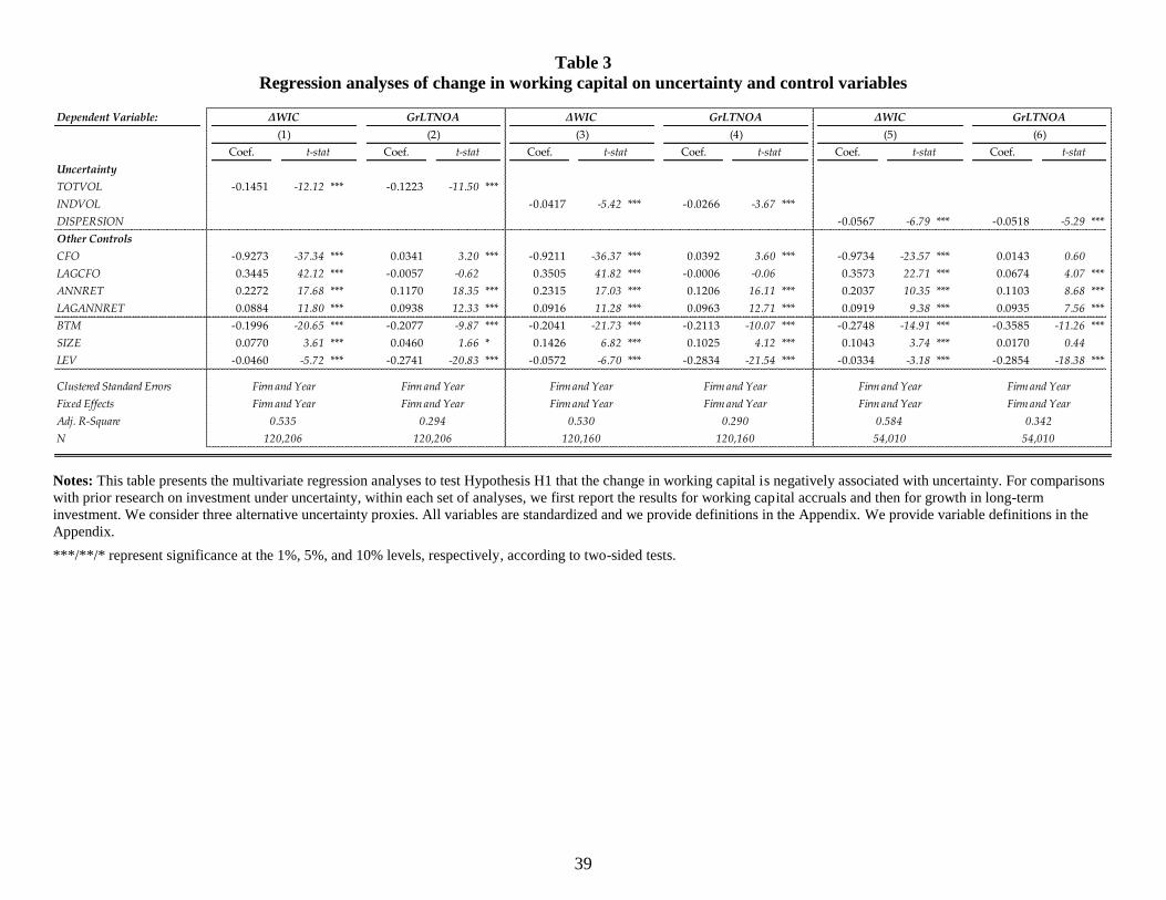
Table 3 provides the results from multivariate analyses to test Hypothesis H1 that
working capital accruals are negatively associated with uncertainty using equation (1).9 The first,
second, and third set of analyses reports the results using total volatility, industry volatility, and
analyst dispersion, respectively. For comparison with prior research on investment under
uncertainty, within each set of analyses, we first report the results for working capital accruals
and then for growth in long-term investment.
First turning to the relation between working capital accruals and uncertainty, we find an
adjusted R2 of 0.535 when total volatility, 0.530 when industry volatility, and 0.584 when analyst
dispersion are used as proxies for uncertainty. For all three measures of uncertainty, we find
9 We also examined the relation between operating accruals and uncertainty. In untabulated results, we find a
significant negative relation between operating accruals and uncertainty.
Page 21
19
significant positive coefficients on LAGCFO, ANNRET and LAGANNRET, which is consistent
with prior research on investment behavior (Eisdorfer, 2008; Hayashi, 1982). This suggests that
firms invest more in working capital accruals when they experience greater prior cash flow
performance and greater current and prior stock return performance. We also find a significant
negative coefficient on CFO, suggesting that companies have smaller working capital accruals
when they experience larger current cash flows from operations. This finding is consistent with
the findings in prior research on accruals (e.g., Fairfield et. al., 2003). We find a significant
negative coefficient on BTM, which is consistent with prior research on investment behavior
(Eisdorfer, 2008) and suggests that firms exhibit greater working capital investment when they
experience higher expected growth. We find a significant positive coefficient on SIZE, which is
consistent with Eisdorfer (2008). Finally, we find a significant negative coefficient on LEV and
working capital accruals, suggesting that companies invest less in working capital accruals in
periods in which their leverage is higher.
The first column in Table 3 provides the results with total volatility included in the model
as a proxy for uncertainty. Consistent with our hypothesis, we find a negative coefficient of -
0.1451 on TOTVOL which is significant at the one percent significance level. In column (3), we
present the results with industry volatility included as the proxy for uncertainty. Again,
consistent with our first hypothesis, we find a negative coefficient of -0.0417 on INDVOL, which
is significant at the one percent significance level. Finally, column (5) presents the results when
analyst forecast dispersion is included as the measure of uncertainty. We find a coefficient of -
0.0567 on DISPERSION, which is significant at the one percent level. The results, therefore,
provide strong evidence to support our first hypothesis that there is a negative relation between
working capital accruals and the level of uncertainty.
Page 22
20
For comparison to prior research on investment under uncertainty, we also report the
results with growth in long-term net operating assets as the proxy for investment. Consistent with
the prior research, we find a significant negative relation between total volatility, industry
volatility, and analyst dispersion and growth in long-term net operating assets. We also find that
the relation is the same relative magnitude as the relation between uncertainty and working
capital accruals. This provides support for the theory that uncertainty leads to lower investment
and for the notion that working capital accruals at least partially reflect investment decisions.
[please place Table 3 about here]
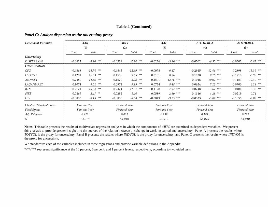
In order to provide greater insight into the sources of the negative relation between
working capital accruals and uncertainty, in Table 4, we present results of regression analyses in
which we examine the components of ∆WIC as the dependent variables. Table 4 provides the
regression results when growth in working capital is further disaggregated into growth in
accounts receivables (∆AR), growth in inventory (∆INV), growth in accounts payable (∆AP),
growth in other current assets (∆OTHERCA), and growth in other current liabilities
(∆OTHERCL). Each dependent and independent variable is standardized so that the coefficients
can be compared across regressions. Panel A, Panel B, and Panel C reports the results with
TOTVOL, INDVOL, and DISPERSION as the proxy for uncertainty, respectively. We find a
negative relation between the asset components (inventory, accounts receivable, other current
assets) and between the liability components (accounts payable, other current liabilities) of
working capital accruals and uncertainty. This suggests that changes in current liabilities do not
behave in an opposite fashion compared to assets with respect to uncertainty, because investment
decisions and growth in the balance sheet are likely to affect current liabilities also. We also find
that the relation is strongest between ∆AR and uncertainty, and then between ∆INV and
Page 23
21
uncertainty when both TOTVOL and INDVOL are used as proxies for uncertainty. The relatively
lower association between uncertainty and other current assets suggest that these items are less
likely to reflect investment. The overall results are consistent with the investment perspective of
accruals and suggest that the relation between working capital accruals and uncertainty is driven
by the level of inventory and accounts receivables. Notably, when DISPERSION is used as the
proxy for uncertainty, the differences in the relations across the components are less pronounced.
[please place Table 4 about here]
In untabulated analyses, we also investigated whether the relation between uncertainty
and working capital accruals is driven by estimated allowance accounts included within the
working capital accounts. For example, the negative relation between uncertainty and changes in
accounts receivables (∆AR) might not be due to firms granting less credit to customers but may
instead be due to firms estimating a greater allowance for bad debts during periods of
uncertainty. To address this possibility, we first separate ∆AR into the change in allowance for
doubtful accounts (∆ADD) and the change in gross accounts receivables (∆GAR). We find that
for companies with non-missing ∆ADD, the mean (median) ∆ADD is 4.1 (1.6) percent of the
mean (median) ∆GAR, suggesting that the estimated allowance is a minor portion of accounts
receivables and, therefore, working capital accruals.
Second, in untabulated analyses, we examine the relation between uncertainty and ∆AR
as well as ∆GAR to assess whether the relations differ. We find that the relation between
uncertainty is similar for ∆GAR and ∆AR. The Pearson (Spearman) correlation between ∆GAR
and TOTVOL, IVOL, and DISPERION is -0.1058 (-0.0978), -0.1040 (-0.0921) and -0.1119 (-
0.1715), respectively which is similar to the correlations for ∆AR reported in Table 2. Finally, in
untabulated regression analyses similar to those reported in Table 4, we find a significant
Page 24
22
coefficient of -0.4748 on TOTVOL and -0.0126 on DISPERSION when (unstandardized) ∆GAR
is the dependent variable and a significant coefficient of -0.4424 on TOTVOL and -0.0109 on
DISPERSION when (unstandardized) ∆AR is the dependent variable. These results suggest that
the negative relation between the change in accounts receivable and uncertainty is not driven by
changes in the allowance for doubtful accounts.
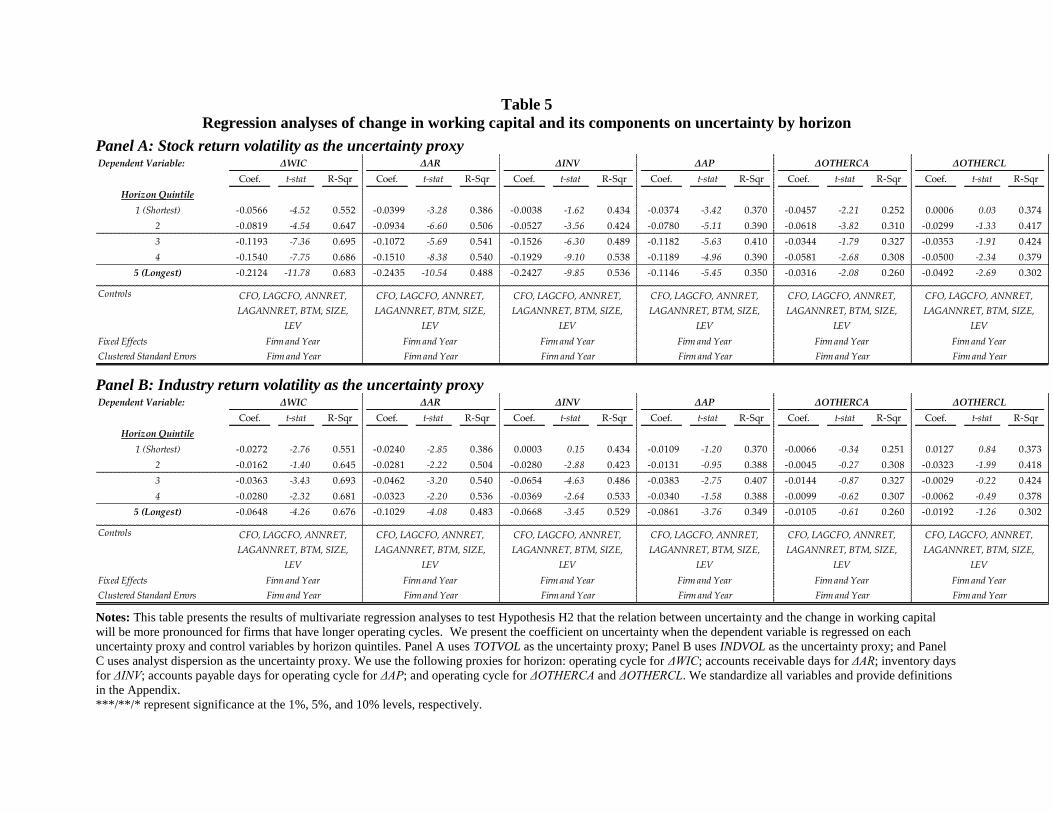
4.2 Test of hypothesis H2
Our second hypothesis predicts that the sensitivity of working capital accruals to
uncertainty is increasing in the length of the firm’s operating cycle. To provide insight into the
validity of this prediction, Table 5 presents the coefficient on uncertainty when ∆WIC is
regressed on each uncertainty proxy and the control variables by operating cycle quintile. The
results are reported when TOTVOL, INDVOL, and DISPERSION are used as the uncertainty
proxy, respectively. Within each set of results, the first column reports the coefficient on the
uncertainty measure, the second column reports the t-statistic for the coefficient, and the third
column reports the adjusted R-squared for the regression. We exclude the coefficients on the
other variables in the regression for brevity. In addition to reporting the relation between
uncertainty and ∆WIC, we report the relation for each of the working capital accrual components.
We find that, for each measure of uncertainty, the coefficient on the uncertainty proxy
generally decreases across the operating cycle quintiles for growth in working capital as well as
for growth in accounts receivable, growth in inventory, and growth in accounts payable. For
example, for total working capital accruals, the coefficient on TOTVOL decreases from -0.0566
for the lowest to -0.2124 for the highest operating cycle quintile and the coefficient on INDVOL
decreases from -0.0272 for the lowest to -0.0648 for the highest operating cycle quintile.
Page 25
23
Similarly, the coefficient on DISPERSION decreases from -0.0225 to -0.0767 across the quintiles
based on the firm’s operating cycle. These results provide strong support for our second
hypothesis that the negative association between working capital accruals and uncertainty
increases as the operating cycle lengthens.
The results for the components of working capital suggest that the influence of the length
of the operating cycle is generally most pronounced for the change in accounts receivables and
the change in inventory than for the other components. This finding is consistent with these
components being more likely to reflect investment decisions and suggests that the relation
between working capital accruals and uncertainty depends on the components of working capital
as well as the length of the operating cycle.
[please place Table 5 about here]
4.3 Test of hypothesis H3
Our third hypothesis predicts a negative relation between abnormal accruals and
uncertainty and that this relation is more pronounced for firms with longer operating cycles. That
is, we examine whether abnormal accruals, a widely used proxy for earnings management, are
systematically related to the uncertainty faced by the firm. We decompose accruals into their
normal and abnormal components and examine the relation of each individual component with
uncertainty. We note at the outset that prior literature expresses concern that standard abnormal
accrual methodologies may be misspecified and assume a stationary accruals generating process;
as a result, they may produce poor proxies for earnings management (e.g. McNichols, 2000;
Gerakos, 2012; Ball, 2013). We use the standard methodologies found in the literature to
Page 26
24
decompose accruals into both the normal and abnormal components and examine the relations to
these components of accruals and uncertainty.
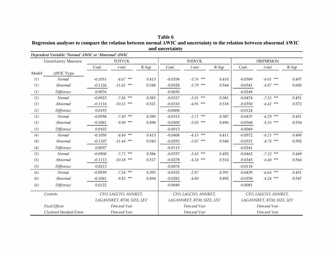
Table 6 presents the results of regressions of normal and abnormal accruals on
uncertainty and control variables. To conserve space, for each regression we report only the
coefficient and t-statistic on the uncertainty proxy (since we are interested in whether normal and
abnormal accruals are associated with uncertainty). The regression adjusted R-squared is also
reported. We run a total of 36 regressions, since we have six abnormal accrual models, two
accrual components (normal and abnormal), and three uncertainty proxies (total return volatility,
industry volatility, and analyst forecast dispersion). To facilitate coefficient comparisons, we
standardize each variable in these regressions. We also report the difference in uncertainty
coefficients across regressions.
Two main results emerge. First, regardless of the accrual decomposition and uncertainty
proxy, there is a negative and statistically significant relation between the accrual measure and
uncertainty. That is, we find that uncertainty is significantly negatively associated with both
normal and abnormal accruals. Second, there is no systematic evidence indicating that the
abnormal accrual-uncertainty relation is stronger than the normal accrual-uncertainty relation.
For each pair of regressions, we compute the difference in uncertainty coefficients across the
normal and abnormal accruals regressions. When the uncertainty proxy is total return volatility,
the abnormal accrual-uncertainty relation is stronger than the normal accrual-uncertainty
relation. However, this flips when using industry volatility and analyst forecast dispersion as the
uncertainty proxy: when industry volatility or analyst forecast dispersion is the uncertainty
proxy, the abnormal accrual-uncertainty relation is weaker than the normal accrual-uncertainty
Page 27
25
relation. In other words, we do not find systematic evidence that the negative accrual-uncertainty
relation is driven by the normal or the abnormal component of accruals.
To summarize, the results of our tests suggest that proxies for earnings management are
systematically associated with the level of uncertainty faced by the firm. Our results tie in neatly
with the predictions of the theoretical investment uncertainty literature that both normal and
abnormal accruals are negatively associated with the level of uncertainty. These results suggest
that earnings management proxies are misspecified and that researchers should take into account
the level of uncertainty faced by the firm when calculating abnormal accruals.
[please place Table 6 here]
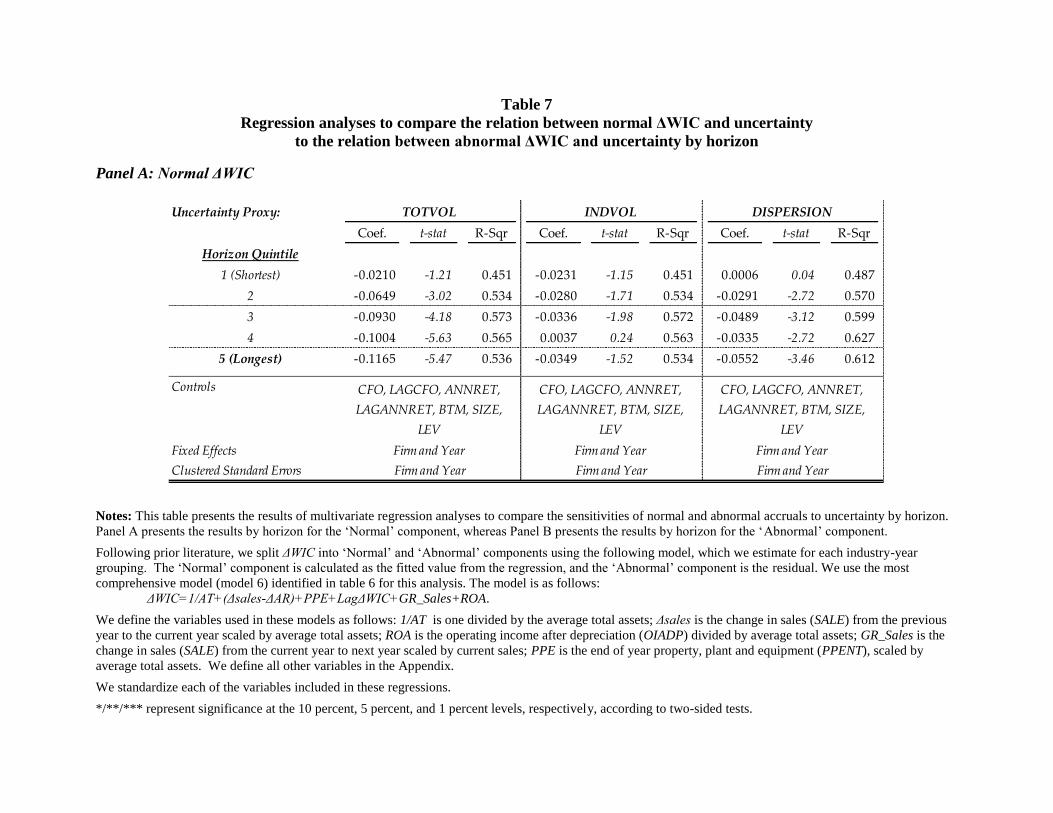
Our third hypothesis also predicts that the negative relation between uncertainty and both
normal and abnormal accruals is increasing in the firm’s operating cycle. For this analysis, we
rely on the most comprehensive abnormal accruals model and report the relation between
uncertainty and the accruals measure by operating cycle quintile. The results are reported in
Table 7. We report the results for normal accruals in panel A and abnormal accruals in panel B.
Within each panel, we report the results for uncertainty proxied by total volatility, industry
volatility, and analyst dispersion, respectively.
Consistent with our hypothesis, we find that the negative coefficient on TOTVOL is
exacerbated as the operating cycle lengthens for both normal and abnormal accruals. We find a
significant negative coefficient on TOTVOL for explaining abnormal accruals for each of the
quintiles and that the coefficient for the longest quintile is three times that for the shortest
quintile. When uncertainty is captured by INDVOL, we also find a generally increasing
coefficient on uncertainty as the operating cycle lengthens for explaining abnormal accruals. In
addition, the coefficient on INDVOL is significant for the highest two operating cycle quintiles.
Page 28
26
When DISPERSION is used to proxy for uncertainty, we find an increase in the coefficients as
the operating cycle lengthens and that the coefficient is significant in all but the lowest operating
cycle quintile.
These results suggest that abnormal accruals models are systematically biased given the
level of uncertainty faced by the firm, and that the bias is more pronounced the longer the firm’s
operating cycle. The findings suggest that research that relies on abnormal accrual models to
proxy for earnings management should consider the negative relation between abnormal accruals
and the level of uncertainty, the components of working capital accruals that comprise accruals,
and the firm’s operating cycle to remove systematic biases from the abnormal accruals measures
that are associated with accruals as a form of investment.
[please place Table7 here]
Our hypotheses are based on the notion that uncertainty drives the level of working
capital accruals rather than the level of working capital accruals driving uncertainty. We address
the problem of endogenetiy in a number of ways. First, we include firm fixed effects in the
regressions to remove firm-level correlated omitted variables that are invariant over the sample
period. This has the added benefit of providing insight into the behavior of accruals vis-a-vis
uncertainty across time for a given firm. Second, we include industry volatility in our tests since
a firm’s level of accruals are unlikely to affect the volatility of stock returns for the industry.
Third, we highlight that if a higher level of accruals leads to a higher level of uncertainty, then
the direction of the relation would be positive instead of negative, as hypothesized in the
investment under uncertainty literature and documented above.
Lastly, we also address the possibility of endogeneity bias by performing analyses where
lagged total stock return volatility (LAGTOTVOL) is used as the proxy for uncertainty. As such,
Page 29
27
it can be considered predetermined (i.e. orthogonal to the current error term), with the associated
coefficient consistently estimated in a large sample (Hayashi, 2000, p.109).10
We find results
(untabulated) that are consistent with those reported in the tables. Specifically, when we run
equation (1), we find a negative coefficient on LAGTOTVOL that is significant at the one percent
level. This indicates that the accrual-uncertainty relation is not driven by a correlated omitted
variable that is contemporaneously associated with both accruals and uncertainty. Second, we
find a monotonically decreasing coefficient on LAGTOTVOL for explaining ∆WIC across
operating cycle quintiles. These results are consistent with those reported in the tables and
suggest that our results are not driven by endogeneity bias.
5. Conclusions
In the real world, firms cannot perfectly forecast the future. The business environment is
continually evolving, and information arrives gradually. Firms must therefore make investment
decisions in the face of uncertainty. In this study, we view working capital accruals as a form of
investment and examine whether theories in finance on investment under uncertainty are
informative about the relation between accruals and uncertainty. In particular, we are guided by
the rich extant literature in economics and finance on investment under uncertainty (e.g.
Bernanke, 1983; McDonald and Siegel, 1986; Ingersoll and Ross, 1992; Dixit, 1992; Dixit and
Pindyck, 1994; and Schwartz and Trigeorgis, 2004). To our knowledge, we are the first to link
the literature on accounting accruals with the literature on investment under uncertainty.
The theory predicts a negative relation between investment and uncertainty because firms
become more cautious about investing when uncertainty is higher. Consistent with this, we
10
Hennessy et al. (2007) use a similar line of reasoning.
Page 30
28
document a significant negative relation between working capital accruals and uncertainty.
Furthermore, we find that inventory and accounts receivable have the highest sensitivity to
uncertainty and that the negative relation between accounts receivables and uncertainty is not
driven by changes in the allowance for bad debts. These results support the view that working
capital accruals reflect investment decisions and that these decisions are associated with the level
uncertainty faced by the firm. We also predict and find that the negative relation between
working capital accruals and uncertainty is more pronounced for firms with longer operating
cycles.
We believe that our findings provide important contributions to the accounting literature
on accruals and to the economics and finance literature on investment and uncertainty.
Specifically, we believe that our findings are an important initial step in understanding the
factors that drive a firm’s level of accruals. Given that accruals are central to the accounting
discipline, understanding the factors that shape the level of a firm’s accruals is of great
importance.
Furthermore, we believe that viewing accruals as a form of investment and taking into
account the role of uncertainty in understanding accruals has the potential to provide insight into
when the extant abnormal accrual models are likely to be systematically biased. As recent
research points out, extant approaches to modeling expected accruals are generally ad hoc,
supported by little theory, and assume stationarity in the accrual process over time and within
industries (e.g. McNichols, 2000; Gerakos, 2012; Ball, 2013, Owens, et al., 2013). Exploiting the
fact that accruals are a form of investment - and drawing on the rich theory provided by the
investment under uncertainty literature – can aid researchers in removing these biases from the
earnings management proxies.
Page 31
29
Our findings also contribute to the economics and finance literature on investment under
uncertainty. This literature has focused on firms’ long-term investment decisions. In contrast,
accrual-based investment has received little attention in this literature. We believe that
distinguishing between accruals and long-term investment provides a fertile testing ground for
assessing the validity of various theories that have been proposed in the literature on investment
under uncertainty.
A variety of other avenues for future research remain. In particular, future research could
examine other measures of uncertainty to determine how different aspects of investment and
accruals relate to uncertainty. For example, research could distinguish between shorter term and
longer term measures of uncertainty. Incorporating other aspects of the economic environment to
further improve models of expected accruals would also be fruitful. We hope to shed light on
some of these aspects in future work.
Page 32
30
References
Allen, E., Larson, C., Sloan, R., 2013.Accrual reversals, earnings, and stock returns. Journal of
Accounting and Economics 56 (1), 113-129.
Ang, A., Hodrick, R., Xing,Y., Zhang, X., 2006. The cross-section of volatility and expected
returns. The Journal of Finance 61, 259-299.
Ball, R., 2013. Accounting informs investors and earnings management is rife: Two questionable
beliefs. Accounting Horizons, forthcoming.
Barro, R,.1990. The stock market and investment. 1990. Review of Financial Studies 3, 115-131.
Bernanke, B., 1983. Irreversibility, uncertainty, and cyclical investment. The Quarterly Journal
of Economics 98, 85-106.
Bloom, N., 2009. The impact of uncertainty shocks. Econometrica 77, 623-685.
Bloom, N., Bond, S., Van Reenen, J., 2007. Uncertainty and investment dynamics. Review of
Economic Studies 74, 391-415.
Bond, S., Cummins, J., 2004. Uncertainty and investment: An empirical investigation using data
on analysts” profit forecasts.” Unpublished paper, Federal Reserve Board.
Bushman, R., Smith, A., Zhang, F., 2011. Investment cash flow sensitivities really reflect related
investment decisions. Unpublished paper.
Caballero, R., 1991. On the sign of the investment-uncertainty relationship. American Economic
Review 81, 279-28.
Chen, C., Huang, A., Jha, R., 2012. Idiosyncratic return volatility and the information quality
underlying managerial discretion. Journal of Financial and Quantitative Analysis 47,
873-899.
DeAngelo, L., 1986. Accounting numbers as market valuation substitutes: A study of
management buyouts of public stockholders. The Accounting Review 61, 400-420.
Dechow, P., 1994. Accounting earnings and cash flows as measures of firm performance: The
role of accounting accruals. Journal of Accounting and Economics 18, 3-42.
Dechow, P., Dichev, I., 2002. The quality of accruals and earnings: The role of accrual
estimation errors. The Accounting Review 77, 35-59.
Dechow, P., Hutton, A., Kim, J., Sloan, R. Detecting Earnings Management: A New Approach.
Journal of Accounting Research 50, 275-334
Dechow, P., Richardson, S., Tuna, I., 2003. Why are earnings kinky? An
examination of the earnings management explanation. Review of Accounting Studies 8,
355-384.
Page 33
31
Dechow, P., Sloan, R., Sweeney, A., 1995. Detecting earnings management. The Accounting
Review 70, 193-225.
Diether, K., Malley, C., Scherbina, A., 2002. Differences of opinion and the cross section of
stock returns. The Journal of Finance 57, 2113-2141.
Dixit, A., 1992. Investment and hysteresis. Journal of Economic Perspectives 6, 107-132.
Dixit, A., Pindyck, R., 1994. Investment under uncertainty. Princeton, NJ: Princeton University
Press.
Eisdorfer, A., 2008. Empirical evidence of risk shifting in financially distressed firms. The
Journal of Finance 63, 609-637.
Fairfield, P., Whisenant, S., Yohn, T., 2003. Accrued earnings and growth: Implications for
future earnings performance and market mispricing.” The Accounting Review 78, 353-
371.
Fama, E., French, K., 1993. Common risk factors in the returns on stocks and bonds. Journal of
Financial Economics 33, 3-56.
Ferderer, J., 1993. The impact of uncertainty on aggregate investment spending: An empirical
analysis. Journal of Money, Credit and Banking 25, 30-48.
Galai, D., Masulis, R., 1976. The option pricing model and the risk factor of stock. Journal of
Financial Economics 3, 53–81.
Gerakos, J., 2012. Discussion of detecting earnings management: A new approach. Journal of
Accounting Research 50, 335-347.
Ghosh, D., Olsen, L., 2009. Environmental uncertainty and managers’ use of discretionary
accruals. Accounting Organizations and Society 34, 83-205.
Grenadier, S., Malenko, A., 2010. A bayesian approach to real options: The case of
distinguishing between temporary and permanent shocks. Journal of Finance 65, 1949-
1986.
Guiso, L. Parigi, G., 1999. Investment and demand uncertainty. Quarterly Journal of Economics
114, 185-227.
Hayashi, F., 1982. Tobin’s marginal q and average q: A neoclassical interpretation.
Econometrica 50, 213-224.
Hayashi, F., 2000. Econometrics. Princeton University Press.
Healy, P., 1985. The effect of bonus schemes on accounting decisions. Journal of Accounting
and Economics 7, 85-107.
Page 34
32
Healy, P., Wahlen, J., 1999. A review of the earnings management literature and its implications
for standard setting. Accounting Horizons 13, 365–383
Hennessy, C., Levy, A., Whited, T. 2007. Testing Q theory with financing frictions. Journal of
Financial Economics 83, 691-717.
Hribar, P., Collins, D., 2002. Errors in estimating accruals: Implications for empirical research.
Journal of Accounting Research 40, 105-134.
Ingersoll, J., Ross, S., 1992. Waiting to invest: Investment and uncertainty. The Journal of
Business 65, 1-29.
Jensen, M., Meckling, W., 1976. Theory of the firm: Managerial behavior, agency
costs and ownership structure. Journal of Financial Economics 3, 305–360.
Jones, J., 1991. Earnings management during import relief investigations. Journal of Accounting
Research 29, 193-229.
Lamont, O., 1997. Cash flow and investment: Evidence from internal capital markets. Journal of
Finance 52, 83-109.
Leahy, J., Whited, T., 1996. The effects of uncertainty on investment: Some stylized facts.
Journal of Money, Credit and Banking 28, 64-83.
McDonald, R., Siegel, D., 1986. The value of waiting to invest. Quarterly Journal of Economics
101, 707-727.
McNichols, M., 2000. Research design issues in earnings management studies. Journal of
Accounting and Public Policy 19, 313-345.
Minton, B., Schrand, D., 1999. The impact of cash flow volatility on discretionary investment
and the costs of debt and equity financing. Journal of Financial Economics 54, 423-460.
Momente, F., Reggiani, F., Richardson, S., 2013. Inventory growth and future performance: Can
it be attributed to risk? Working paper.
Owens, E., Wu, J., Zimmerman, J. 2013. Business model shocks and abnormal accrual models.
Working paper.
Richardson, S., Sloan, R., Soliman, M., Tuna, I., 2005. Accrual reliability, earnings persistence,
and stock prices. Journal of Accounting and Economics 39, 437-485.
Schwartz, E., Trigeorgis, L., 2004. Real Options and Investment Uncertainty: Classical
Readings and Recent Contributions. Cambridge, MA: MIT Press.
Sloan, R., 1996. Do stock prices fully reflect information in accruals and cash flows about future
earnings? The Accounting Review 71, 289-315.
Wu, J., Zhang, L., Zhang, X., 2010. The q-theory approach to understanding the accrual
anomaly. Journal of Accounting Research 48, 177-224.
Page 35
33
Xie, H., 2001. The mispricing of abnormal accruals. The Accounting Review 76, 357-373.
Zang, A. 2012. Evidence on the trade-off between real activities manipulation and accrual-based
earnings management. The Accounting Review 87, 675-703.
Zhang, X., 2007. Accruals, investment, and the accrual anomaly. The Accounting Review 82,
1333-1363.
Page 36
34
Appendix
Variable definitions
Variable Definition of Variable
Uncertainty Variables:
TOTVOL Stock return volatility, calculated as the standard deviation of daily returns
over the current fiscal year for the firm’s stock.
LAGTOTVOL Lagged return volatility, calculated as the standard deviation of daily
returns over the prior fiscal year for the firm’s stock.
INDVOL Industry stock return volatility, calculated as the standard deviation of
daily returns over the current fiscal year for an equal-weighted portfolio of
stocks in the same 4-digit SIC code.
DISPERSION Analyst earnings forecast dispersion, calculated as of the fourth month of
the fiscal year. DISPERSION is calculated as the standard deviation of
analyst earnings estimates for the current fiscal year divided by the
absolute value of the mean of the same estimates.
Accrual/Investment Variables:
ΔAR Change in accounts receivable (RECT), scaled by average total assets.
ΔINV Change in inventories (INVT), scaled by average total assets.
ΔAP Change in accounts payable (AP), scaled by average total assets.
ΔOTHERCA Change in other current assets (ACO), scaled by average total assets.
ΔOTHERNCA Change in other current liabilities (LCO), scaled by average total assets.
ΔWIC Growth (net change) in operating working capital, scaled by average total
assets: ΔWIC=(ΔAR+ ΔINV+ ΔOTHERCA)-(ΔAP+ ΔOTHERCL).
GrLTNOA Growth in long-term net operating assets, i.e. growth in net operating
assets less growth in working capital, scaled by average total assets.
GrLTNOA is defined following Fairfield et. al. (2003) as
ΔPPE+ΔINTANG+ΔAO-ΔLO and is scaled by average total assets
Control Variables:
CFO Cash flow from operations, as defined in Fairfield et. al. (2003), or
operating income less accruals, scaled by average total assets. Operating
income is defined as operating income after depreciation and amortization
(OIADP). Formally, CFO=(OIADP/avg. tot. assets)-ACC.
LAGCFO CFO for the prior fiscal year.
Page 37
35
ANNRET The current fiscal year return for the firm’s stock, calculated by
compounding monthly CRSP returns.
LAGANNRET The prior fiscal year’s return for the firm’s stock.
BTM Book-to-market ratio, calculated at the beginning of the fiscal year. BTM
is calculated as the ratio of equity book value (CEQ) to the equity market
value, per CRSP.
SIZE Natural log of the market value of equity for the firm at the beginning of
the fiscal year.
LEV Leverage at the beginning of the fiscal year, calculated as the book value of
total debt (DLC+DLTT) divided by the book value of total assets (AT).
Horizon Variables:
OPERCYCLE Operating cycle, as defined in Dechow (1994), or average accounts
receivable divided by (sales/360), plus average inventory divided by (cost
of goods sold/360).
AR_DAYS Accounts receivable days, or average accounts receivable divided by
(sales/360).
INV_DAYS Inventory days, or average inventory divided by (cost of goods sold/360).
AP_DAYS Accounts payable days, or average accounts payable divided by
(purchases/360), where purchases is cost of good sold plus ΔINV.
Page 38
36
Table 1
Sample selection
Notes: This table presents an overview of the sample selection procedure. The table begins with the total number of observations on
Compustat from 1965 to 2010 that meet the data requirements for the dependent and explanatory variables. We then narrow the
population to observations that meet the CRSP data requirements for U.S. ordinary common share firms. This results in the total
sample for analyses where return volatility proxies for uncertainty. Next, we require at least two analyst forecasts for each firm-year
observations. This yields the total sample for analyses where analyst dispersion proxies for uncertainty.
SAMPLE
Reductions
Cumulative
SAMPLE
Total
Observations that meet COMPUSTAT requirements
(i.e., Fairfield et. al. 2003 accrual variable requirements) [1965 - 2010] 181,064
No Link to CRSP (48,512) 132,552
Include Only Ordinary Common Shares in U.S. Incorporated Companies (SHRCD='10' or '11' ) (6,296) 126,256
SIZE, BTM at beginning of FY not available (5,870) 120,386
Components to calculate Z_SCORE at beginning of year not available (138) 120,248
Returns Unvailable in Monthly Stock File (7) 120,241
Volatility Measures Not Available (35) 120,206
120,206
Total sample for analyses where return volatility proxies for uncertainty 120,206
Require at least 2 analyst forecasts (66,196) 54,010
Total sample for analyses where analyst dispersion proxies for uncertainty 54,010
Page 39
37
Table 2
Descriptive statistics and correlations
Panel A: Descriptive statistics
Notes: This panel presents descriptive statistics. We provide variable definitions in the Appendix. We winsorize each variable at the 1 percent and 99 percent levels.
n Mean Median
First
Quartile
Third
Quartile Min Max Std Dev
Uncertainty Variables
TOTVOL 120,206 0.0359 0.0305 0.0208 0.0448 0.0088 0.1205 0.0214
INDVOL 120,160 0.0168 0.0142 0.0104 0.0202 0.0041 0.0588 0.0098
DISPERSION 54,010 0.1740 0.0571 0.0265 0.1429 0.0000 2.7778 0.3829
Accrual/Investment Variables
ΔAR 120,206 0.0176 0.0097 -0.0081 0.0407 -0.2126 0.2858 0.0691
ΔINV 120,206 0.0133 0.0014 -0.0032 0.0282 -0.1895 0.2505 0.0597
ΔAP 120,206 0.0095 0.0050 -0.0071 0.0226 -0.1310 0.1856 0.0431
ΔOTHERCA 120,206 0.0031 0.0012 -0.0023 0.0076 -0.0782 0.0937 0.0201
ΔOTHERCL 120,206 0.0102 0.0054 -0.0040 0.0211 -0.1242 0.1789 0.0396
ΔWIC 120,206 0.0143 0.0090 -0.0234 0.0520 -0.3135 0.3383 0.0939
GrLTNOA 120,206 0.0394 0.0181 -0.0150 0.0740 -0.4079 0.6495 0.1400
Control Variables
CFO 120,206 0.0783 0.1100 0.0275 0.1787 -0.8076 0.4613 0.1918
LAGCFO 120,206 0.0758 0.1099 0.0248 0.1796 -0.8425 0.4691 0.1989
ANNRET 120,206 0.1579 0.0575 -0.2333 0.3808 -0.8286 3.1250 0.6398
LAGANNRET 120,206 0.1540 0.0456 -0.2273 0.3675 -0.8088 3.1150 0.6311
BTM 120,206 0.8031 0.6081 0.3263 1.0558 -0.2956 3.9096 0.7182
SIZE 120,206 4.5165 4.3518 2.8669 6.0223 0.2889 10.0314 2.1650
LEV 120,206 0.2345 0.2137 0.0559 0.3623 0.0000 0.8337 0.1962
Horizon Variables
OPERCYCLE 119,167 153.5 117.3 73.0 178.5 7.0 1,269.5 163.0
AR_DAYS 119,303 69.5 53.7 36.6 73.9 0.1 708.8 87.1
INV_DAYS 119,364 77.9 58.5 14.7 108.3 0.0 539.2 87.4
AP_DAYS 119,524 58.8 35.1 23.0 53.6 2.7 759.2 98.0
Page 40
38
Table 2 (Continued)
Panel B: Univariate correlations (Spearman coefficients in the upper triangle; Pearson coefficients in the lower triangle)
Notes: This panel presents univariate correlations. Spearman correlation coefficients are in the upper triangle and Pearson correlation coefficients are in the lower triangle. We
provide variable definitions in the Appendix.
Variable (1) (2) (3) (4) (5) (6) (7) (8) (9) (10) (11) (12) (13) (14) (15) (16) (17) (18) (19) (20) (21)
(1) TOTVOL 1 0.390 0.340 -0.080 -0.110 -0.060 -0.030 -0.040 -0.070 -0.170 -0.330 -0.360 -0.210 -0.260 -0.110 -0.420 -0.060 0.100 0.160 -0.010 0.160
(2) INDVOL 0.380 1 0.080 -0.060 -0.040 -0.050 -0.010 -0.040 -0.030 -0.090 -0.070 -0.070 -0.110 -0.110 -0.060 0.000 -0.020 0.040 0.020 0.020 0.010
(3) DISPERSION 0.250 0.090 1 -0.150 -0.170 -0.090 -0.100 -0.080 -0.150 -0.190 -0.310 -0.320 -0.080 -0.230 0.200 -0.260 0.030 0.030 0.080 -0.010 0.090
(4) ΔAR -0.090 -0.060 -0.100 1 0.320 0.440 0.150 0.330 0.560 0.300 -0.110 0.080 0.170 0.180 -0.130 0.010 -0.080 0.010 0.060 -0.020 -0.050
(5) ΔINV -0.100 -0.050 -0.110 0.310 1 0.380 0.130 0.210 0.560 0.300 -0.130 0.090 0.090 0.180 -0.080 0.010 -0.060 0.080 -0.100 0.180 -0.100
(6) ΔAP -0.060 -0.040 -0.070 0.470 0.420 1 0.150 0.200 0.090 0.300 0.020 0.040 0.120 0.130 -0.070 0.000 -0.040 -0.040 -0.050 -0.010 0.020
(7) ΔOTHERCA -0.040 -0.020 -0.070 0.100 0.070 0.110 1 0.240 0.230 0.180 -0.020 0.090 0.060 0.110 -0.120 0.060 -0.070 -0.030 -0.020 -0.010 -0.030
(8) ΔOTHERCL -0.030 -0.040 -0.060 0.320 0.180 0.170 0.240 1 -0.050 0.250 0.130 0.030 0.130 0.110 -0.110 0.050 -0.080 -0.050 -0.020 -0.030 -0.070
(9) ΔWIC -0.100 -0.050 -0.100 0.600 0.620 0.090 0.230 -0.120 1 0.180 -0.330 0.100 0.080 0.150 -0.090 -0.020 -0.060 0.090 0.010 0.110 -0.090
(10) GrLTNOA -0.120 -0.060 -0.110 0.260 0.220 0.270 0.120 0.240 0.120 1 0.130 0.180 0.090 0.220 -0.190 0.140 -0.070 -0.110 -0.080 -0.070 -0.030
(11) CFO -0.370 -0.060 -0.180 -0.140 -0.160 -0.020 -0.040 0.090 -0.290 0.080 1 0.570 0.230 0.150 -0.010 0.210 0.080 -0.190 -0.210 -0.050 -0.140
(12) LAGCFO -0.380 -0.060 -0.180 0.030 0.040 -0.010 0.050 -0.030 0.090 0.080 0.690 1 0.140 0.210 -0.040 0.230 -0.020 -0.210 -0.220 -0.070 -0.160
(13) ANNRET -0.040 -0.050 -0.020 0.160 0.090 0.110 0.050 0.110 0.090 0.080 0.130 0.060 1 0.000 0.170 -0.020 0.010 -0.060 -0.070 -0.020 -0.060
(14) LAGANNRET -0.140 -0.060 -0.120 0.140 0.150 0.110 0.090 0.090 0.130 0.170 0.070 0.110 -0.050 1 -0.240 0.210 -0.050 -0.060 -0.070 -0.030 -0.070
(15) BTM 0.010 0.010 0.120 -0.120 -0.090 -0.060 -0.070 -0.090 -0.100 -0.170 0.080 0.060 0.150 -0.240 1 -0.360 0.110 0.060 -0.050 0.120 -0.140
(16) SIZE -0.390 -0.030 -0.160 0.000 -0.010 -0.010 0.040 0.030 -0.010 0.080 0.180 0.200 -0.090 0.130 -0.390 1 -0.030 -0.140 -0.070 -0.120 0.020
(17) LEV 0.000 0.020 0.040 -0.080 -0.070 -0.050 -0.050 -0.070 -0.060 -0.060 0.100 0.020 0.010 -0.060 0.060 -0.040 1 -0.050 -0.070 0.020 0.030
(18) OPERCYCLE 0.110 0.040 0.020 -0.020 0.010 -0.030 -0.020 -0.040 0.010 -0.070 -0.190 -0.210 -0.040 -0.040 0.030 -0.080 0.030 1 0.590 0.780 0.310
(19) AR_DAYS 0.110 0.030 0.020 0.020 -0.070 -0.010 -0.020 -0.020 -0.030 -0.050 -0.180 -0.190 -0.030 -0.020 -0.020 -0.020 0.020 0.750 1 0.090 0.310
(20) INV_DAYS 0.060 0.020 0.010 -0.060 0.080 -0.040 -0.010 -0.050 0.050 -0.070 -0.100 -0.120 -0.030 -0.040 0.060 -0.110 0.010 0.680 0.110 1 0.150
(21) AP_DAYS 0.140 0.000 0.070 -0.030 -0.090 0.030 -0.020 -0.030 -0.090 0.010 -0.140 -0.150 -0.020 -0.020 -0.080 -0.020 0.010 0.360 0.410 0.130 1
Page 41
39
Table 3
Regression analyses of change in working capital on uncertainty and control variables
Notes: This table presents the multivariate regression analyses to test Hypothesis H1 that the change in working capital is negatively associated with uncertainty. For comparisons
with prior research on investment under uncertainty, within each set of analyses, we first report the results for working capital accruals and then for growth in long-term
investment. We consider three alternative uncertainty proxies. All variables are standardized and we provide definitions in the Appendix. We provide variable definitions in the
Appendix.
***/**/* represent significance at the 1%, 5%, and 10% levels, respectively, according to two-sided tests.
Dependent Variable:
Coef. Coef. Coef. Coef. Coef. Coef.
Uncertainty
TOTVOL -0.1451 -12.12 *** -0.1223 -11.50 ***
INDVOL -0.0417 -5.42 *** -0.0266 -3.67 ***
DISPERSION -0.0567 -6.79 *** -0.0518 -5.29 ***
Other Controls
CFO -0.9273 -37.34 *** 0.0341 3.20 *** -0.9211 -36.37 *** 0.0392 3.60 *** -0.9734 -23.57 *** 0.0143 0.60
LAGCFO 0.3445 42.12 *** -0.0057 -0.62 0.3505 41.82 *** -0.0006 -0.06 0.3573 22.71 *** 0.0674 4.07 ***
ANNRET 0.2272 17.68 *** 0.1170 18.35 *** 0.2315 17.03 *** 0.1206 16.11 *** 0.2037 10.35 *** 0.1103 8.68 ***
LAGANNRET 0.0884 11.80 *** 0.0938 12.33 *** 0.0916 11.28 *** 0.0963 12.71 *** 0.0919 9.38 *** 0.0935 7.56 ***
BTM -0.1996 -20.65 *** -0.2077 -9.87 *** -0.2041 -21.73 *** -0.2113 -10.07 *** -0.2748 -14.91 *** -0.3585 -11.26 ***
SIZE 0.0770 3.61 *** 0.0460 1.66 * 0.1426 6.82 *** 0.1025 4.12 *** 0.1043 3.74 *** 0.0170 0.44
LEV -0.0460 -5.72 *** -0.2741 -20.83 *** -0.0572 -6.70 *** -0.2834 -21.54 *** -0.0334 -3.18 *** -0.2854 -18.38 ***
Clustered Standard Errors
Fixed Effects
Adj. R-Square
N
Firm and Year
(6)
ΔWIC GrLTNOA
(3) (4)
t-stat t-stat
Firm and Year Firm and Year
Firm and Year Firm and YearFirm and Year Firm and Year Firm and Year
t-stat t-stat t-stat
54,010
0.535
120,206 120,206 54,010120,160 120,160
0.3420.530 0.2900.294 0.584
Firm and Year Firm and Year Firm and Year Firm and Year
ΔWIC GrLTNOA ΔWIC
t-stat
(1) (2) (5)
GrLTNOA
Page 42
40
Table 4
Regression analyses to investigate the disaggregation of change in working capital
Panel A: Stock return volatility as the uncertainty proxy
Notes: This table presents the results of multivariate regression analyses in which the components of ΔWIC are examined as dependent variables. We present this analysis to
provide greater insight into the sources of the relation between the change in working capital and uncertainty. Panel A presents the results where TOTVOL is the proxy for
uncertainty; Panel B presents the results where INDVOL is the proxy for uncertainty; and Panel C presents the results where INDVOL is the proxy for uncertainty.
We standardize each of the variables included in these regressions and provide variable definitions in the Appendix.
*/**/*** represent significance at the 10 percent, 5 percent, and 1 percent levels, respectively, according to two-sided tests.
Dependent Variable:
Coef. Coef. Coef. Coef. Coef.
Uncertainty
TOTVOL -0.1497 -15.74 *** -0.1401 -12.48 *** -0.1082 -12.14 *** -0.0532 -7.27 *** -0.0425 -4.19 ***
Other Controls
CFO -0.4746 -22.17 *** -0.5094 -16.26 *** -0.0537 -4.54 *** -0.2064 -16.68 *** 0.2281 15.67 ***
LAGCFO 0.1195 12.76 *** 0.1504 12.84 *** -0.0189 -2.14 ** 0.1049 10.35 *** -0.1591 -13.97 ***
ANNRET 0.2441 22.65 *** 0.1979 12.57 *** 0.1422 15.48 *** 0.0943 13.86 *** 0.1129 17.11 ***
LAGANNRET 0.0972 12.40 *** 0.1018 11.78 *** 0.0783 10.77 *** 0.0594 11.01 *** 0.0606 8.87 ***
BTM -0.1483 -15.37 *** -0.1692 -15.86 *** -0.0589 -7.79 *** -0.0258 -2.50 ** -0.0181 -2.92 ***
SIZE 0.0365 2.16 ** 0.0585 3.52 *** -0.0290 -1.90 * 0.1415 8.20 *** 0.0855 5.18 ***
LEV -0.0654 -9.21 *** -0.1152 -12.33 *** -0.0932 -14.16 *** -0.0290 -3.88 *** -0.0819 -12.80 ***
Clustered Standard Errors
Fixed Effects
Adj. R-Square
N
ΔAR ΔINV ΔOTHERCA
(4)
t-stat
Firm and Year
Firm and Year
0.132
120,206
ΔAP ΔOTHERCL
(1) (2) (3) (5)
t-stat t-stat t-stat t-stat
Firm and Year Firm and Year Firm and Year Firm and Year
Firm and Year Firm and Year Firm and Year Firm and Year
0.339 0.353 0.206 0.211
120,206 120,206 120,206 120,206
Page 43
Table 4 (Continued)
Panel B: Industry return volatility as the uncertainty proxy
Notes: This table presents the results of multivariate regression analyses in which the components of ΔWIC are examined as dependent variables. We present
this analysis to provide greater insight into the sources of the relation between the change in working capital and uncertainty. Panel A presents the results where
TOTVOL is the proxy for uncertainty; Panel B presents the results where INDVOL is the proxy for uncertainty; and Panel C presents the results where INDVOL is
the proxy for uncertainty.
We standardize each of the variables included in these regressions and provide variable definitions in the Appendix.
*/**/*** represent significance at the 10 percent, 5 percent, and 1 percent levels, respectively, according to two-sided tests.
Dependent Variable:
Coef. Coef. Coef. Coef. Coef.
Uncertainty
INDVOL -0.0456 -5.00 *** -0.0455 -5.76 *** -0.0369 -5.00 *** -0.0081 -1.19 -0.0115 -1.61
Other Controls
CFO -0.4681 -21.48 *** -0.5036 -15.96 *** -0.0491 -4.13 *** -0.2039 -16.63 *** 0.2300 15.74 ***
LAGCFO 0.1257 13.65 *** 0.1558 13.26 *** -0.0150 -1.66 * 0.1071 10.35 *** -0.1572 -13.87 ***
ANNRET 0.2485 21.29 *** 0.2021 12.33 *** 0.1454 15.09 *** 0.0960 13.57 *** 0.1142 16.85 ***
LAGANNRET 0.1004 12.12 *** 0.1049 11.83 *** 0.0808 11.06 *** 0.0604 10.69 *** 0.0613 9.10 ***
BTM -0.1529 -15.97 *** -0.1735 -16.76 *** -0.0621 -8.45 *** -0.0274 -2.66 *** -0.0195 -3.19 ***
SIZE 0.1037 6.13 *** 0.1218 7.30 *** 0.0200 1.49 0.1669 10.07 *** 0.1048 7.41 ***
LEV -0.0770 -10.43 *** -0.1257 -12.65 *** -0.1014 -14.96 *** -0.0331 -4.42 *** -0.0850 -13.22 ***
Clustered Standard Errors
Fixed Effects
Adj. R-Square
N
ΔOTHERCAΔAR ΔINV ΔAP ΔOTHERCL
(1) (2) (3) (5)
t-stat t-stat t-stat t-stat
(4)
t-stat
Firm and Year Firm and Year Firm and Year Firm and YearFirm and Year
120,160 120,160 120,160 120,160
0.131
120,160
Firm and Year Firm and Year Firm and Year Firm and YearFirm and Year
0.334 0.348 0.203 0.211
Page 44
Table 4 (Continued)
Panel C: Analyst dispersion as the uncertainty proxy
Notes: This table presents the results of multivariate regression analyses in which the components of ΔWIC are examined as dependent variables. We present
this analysis to provide greater insight into the sources of the relation between the change in working capital and uncertainty. Panel A presents the results where
TOTVOL is the proxy for uncertainty; Panel B presents the results where INDVOL is the proxy for uncertainty; and Panel C presents the results where INDVOL is
the proxy for uncertainty.
We standardize each of the variables included in these regressions and provide variable definitions in the Appendix.
*/**/*** represent significance at the 10 percent, 5 percent, and 1 percent levels, respectively, according to two-sided tests.
Dependent Variable:
Coef. Coef. Coef. Coef. Coef.
Uncertainty
DISPERSION -0.0422 -5.90 *** -0.0539 -7.24 *** -0.0226 -3.96 *** -0.0502 -6.55 *** -0.0302 -3.82 ***
Other Controls
CFO -0.4868 -14.74 *** -0.4843 -12.69 *** -0.0078 -0.47 -0.2945 -12.46 *** 0.2898 13.39 ***
LAGCFO 0.1281 10.03 *** 0.1559 9.65 *** 0.0131 0.96 0.1938 8.70 *** -0.1718 -9.99 ***
ANNRET 0.2480 14.56 *** 0.1670 8.98 *** 0.1501 12.76 *** 0.1016 10.02 *** 0.1153 12.30 ***
LAGANNRET 0.1074 9.51 *** 0.0971 9.15 *** 0.0724 8.48 *** 0.0624 7.13 *** 0.0700 6.28 ***
BTM -0.2171 -15.34 *** -0.2424 -11.91 *** -0.1128 -7.97 *** -0.0748 -3.67 *** -0.0404 -3.36 ***
SIZE 0.0469 2.47 ** 0.0292 1.40 -0.0589 -2.69 *** 0.1146 4.29 *** 0.0219 0.71
LEV -0.0835 -9.15 *** -0.0830 -8.58 *** -0.0849 -9.73 *** -0.0333 -3.07 *** -0.1055 -9.08 ***
Clustered Standard Errors
Fixed Effects
Adj. R-Square
N
ΔOTHERCA
(4)
t-stat
Firm and Year
Firm and Year
ΔAR ΔINV ΔAP ΔOTHERCL
t-stat t-stat t-stat t-stat
(1) (2) (3) (5)
Firm and Year Firm and Year Firm and Year Firm and Year
Firm and Year Firm and Year Firm and Year Firm and Year
54,010 54,010 54,010 54,010
0.411 0.413 0.299 0.2850.181
54,010
Page 45
Table 5
Regression analyses of change in working capital and its components on uncertainty by horizon
Panel A: Stock return volatility as the uncertainty proxy
Panel B: Industry return volatility as the uncertainty proxy
Notes: This table presents the results of multivariate regression analyses to test Hypothesis H2 that the relation between uncertainty and the change in working capital
will be more pronounced for firms that have longer operating cycles. We present the coefficient on uncertainty when the dependent variable is regressed on each
uncertainty proxy and control variables by horizon quintiles. Panel A uses TOTVOL as the uncertainty proxy; Panel B uses INDVOL as the uncertainty proxy; and Panel
C uses analyst dispersion as the uncertainty proxy. We use the following proxies for horizon: operating cycle for ΔWIC; accounts receivable days for ΔAR; inventory days
for ΔINV; accounts payable days for operating cycle for ΔAP; and operating cycle for ΔOTHERCA and ΔOTHERCL. We standardize all variables and provide definitions
in the Appendix.
***/**/* represent significance at the 1%, 5%, and 10% levels, respectively.
Dependent Variable:
Coef. t-stat R-Sqr Coef. t-stat R-Sqr Coef. t-stat R-Sqr Coef. t-stat R-Sqr Coef. t-stat R-Sqr Coef. t-stat R-Sqr
Horizon Quintile
1 (Shortest) -0.0566 -4.52 0.552 -0.0399 -3.28 0.386 -0.0038 -1.62 0.434 -0.0374 -3.42 0.370 -0.0457 -2.21 0.252 0.0006 0.03 0.374
2 -0.0819 -4.54 0.647 -0.0934 -6.60 0.506 -0.0527 -3.56 0.424 -0.0780 -5.11 0.390 -0.0618 -3.82 0.310 -0.0299 -1.33 0.417
3 -0.1193 -7.36 0.695 -0.1072 -5.69 0.541 -0.1526 -6.30 0.489 -0.1182 -5.63 0.410 -0.0344 -1.79 0.327 -0.0353 -1.91 0.424
4 -0.1540 -7.75 0.686 -0.1510 -8.38 0.540 -0.1929 -9.10 0.538 -0.1189 -4.96 0.390 -0.0581 -2.68 0.308 -0.0500 -2.34 0.379
5 (Longest) -0.2124 -11.78 0.683 -0.2435 -10.54 0.488 -0.2427 -9.85 0.536 -0.1146 -5.45 0.350 -0.0316 -2.08 0.260 -0.0492 -2.69 0.302
Controls
Fixed Effects
Clustered Standard Errors
Firm and Year Firm and Year Firm and Year Firm and Year
Firm and Year Firm and Year Firm and Year Firm and Year Firm and Year
ΔAR ΔINV
Firm and Year Firm and Year
Firm and Year
ΔAP ΔOTHERCA ΔOTHERCL
CFO, LAGCFO, ANNRET,
LAGANNRET, BTM, SIZE,
LEV
CFO, LAGCFO, ANNRET,
LAGANNRET, BTM, SIZE,
LEV
CFO, LAGCFO, ANNRET,
LAGANNRET, BTM, SIZE,
LEV
CFO, LAGCFO, ANNRET,
LAGANNRET, BTM, SIZE,
LEV
CFO, LAGCFO, ANNRET,
LAGANNRET, BTM, SIZE,
LEV
CFO, LAGCFO, ANNRET,
LAGANNRET, BTM, SIZE,
LEV
ΔWIC
Dependent Variable:
Coef. t-stat R-Sqr Coef. t-stat R-Sqr Coef. t-stat R-Sqr Coef. t-stat R-Sqr Coef. t-stat R-Sqr Coef. t-stat R-Sqr
Horizon Quintile
1 (Shortest) -0.0272 -2.76 0.551 -0.0240 -2.85 0.386 0.0003 0.15 0.434 -0.0109 -1.20 0.370 -0.0066 -0.34 0.251 0.0127 0.84 0.373
2 -0.0162 -1.40 0.645 -0.0281 -2.22 0.504 -0.0280 -2.88 0.423 -0.0131 -0.95 0.388 -0.0045 -0.27 0.308 -0.0323 -1.99 0.418
3 -0.0363 -3.43 0.693 -0.0462 -3.20 0.540 -0.0654 -4.63 0.486 -0.0383 -2.75 0.407 -0.0144 -0.87 0.327 -0.0029 -0.22 0.424
4 -0.0280 -2.32 0.681 -0.0323 -2.20 0.536 -0.0369 -2.64 0.533 -0.0340 -1.58 0.388 -0.0099 -0.62 0.307 -0.0062 -0.49 0.378
5 (Longest) -0.0648 -4.26 0.676 -0.1029 -4.08 0.483 -0.0668 -3.45 0.529 -0.0861 -3.76 0.349 -0.0105 -0.61 0.260 -0.0192 -1.26 0.302
Controls
Fixed Effects
Clustered Standard Errors Firm and Year Firm and Year Firm and Year Firm and Year Firm and Year
Firm and Year
Firm and Year
CFO, LAGCFO, ANNRET,
LAGANNRET, BTM, SIZE,
LEV
Firm and Year Firm and Year Firm and Year Firm and Year Firm and Year
CFO, LAGCFO, ANNRET,
LAGANNRET, BTM, SIZE,
LEV
CFO, LAGCFO, ANNRET,
LAGANNRET, BTM, SIZE,
LEV
CFO, LAGCFO, ANNRET,
LAGANNRET, BTM, SIZE,
LEV
CFO, LAGCFO, ANNRET,
LAGANNRET, BTM, SIZE,
LEV
CFO, LAGCFO, ANNRET,
LAGANNRET, BTM, SIZE,
LEV
ΔWIC ΔAR ΔINV ΔAP ΔOTHERCLΔOTHERCA
Page 46
Table 5 (Continued)
Panel C: Analyst dispersion as the uncertainty proxy
Notes: This table presents the results of multivariate regression analyses to test Hypothesis H2 that the relation between uncertainty and the change in working
capital will be more pronounced for firms that have longer operating cycles. We present the coefficient on uncertainty when the dependent variable is regressed
on each uncertainty proxy and control variables by horizon quintiles. Panel A uses TOTVOL as the uncertainty proxy; Panel B uses INDVOL as the uncertainty
proxy; and Panel C uses analyst dispersion as the uncertainty proxy. We use the following proxies for horizon: operating cycle for ΔWIC; accounts receivable
days for ΔAR; inventory days for ΔINV; accounts payable days for operating cycle for ΔAP; and operating cycle for ΔOTHERCA and ΔOTHERCL. We
standardize all variables and provide definitions in the Appendix.
***/**/* represent significance at the 1%, 5%, and 10% levels, respectively.
Dependent Variable:
Coef. t-stat R-Sqr Coef. t-stat R-Sqr Coef. t-stat R-Sqr Coef. t-stat R-Sqr Coef. t-stat R-Sqr Coef. t-stat R-Sqr
Horizon Quintile
1 (Shortest) -0.0225 -1.70 0.602 -0.0293 -3.88 0.416 -0.0015 -1.53 0.398 -0.0167 -1.85 0.424 -0.0467 -2.48 0.284 -0.0322 -1.33 0.424
2 -0.0436 -4.62 0.673 -0.0236 -2.40 0.566 -0.0149 -2.19 0.448 -0.0012 -0.10 0.459 -0.0529 -4.61 0.336 -0.0072 -0.40 0.470
3 -0.0508 -3.75 0.715 -0.0191 -1.45 0.610 -0.0520 -4.22 0.509 -0.0022 -0.15 0.473 -0.0209 -1.48 0.372 -0.0022 -0.14 0.453
4 -0.0570 -3.77 0.747 -0.0190 -1.30 0.603 -0.0860 -4.79 0.566 -0.0196 -1.38 0.489 -0.0825 -4.96 0.355 -0.0307 -1.73 0.455
5 (Longest) -0.0767 -4.52 0.749 -0.0603 -3.67 0.559 -0.0940 -4.70 0.599 -0.0346 -2.23 0.450 -0.0492 -1.99 0.302 -0.0403 -2.40 0.361
Controls
Fixed Effects
Clustered Standard Errors
ΔAP
CFO, LAGCFO, ANNRET,
LAGANNRET, BTM, SIZE,
LEV
Firm and Year
Firm and Year
CFO, LAGCFO, ANNRET,
LAGANNRET, BTM, SIZE,
LEV
Firm and Year
Firm and Year
ΔOTHERCL
CFO, LAGCFO, ANNRET,
LAGANNRET, BTM, SIZE,
LEV
Firm and Year
Firm and YearFirm and Year Firm and Year Firm and Year
CFO, LAGCFO, ANNRET,
LAGANNRET, BTM, SIZE,
LEV
CFO, LAGCFO, ANNRET,
LAGANNRET, BTM, SIZE,
LEV
CFO, LAGCFO, ANNRET,
LAGANNRET, BTM, SIZE,
LEV
Firm and Year Firm and Year Firm and Year
ΔOTHERCAΔWIC ΔAR ΔINV
Page 47
Table 6
Regression analyses to compare the relation between normal ΔWIC and uncertainty to the relation between abnormal ΔWIC
and uncertainty
Uncertainty Measure
Coef. R-Sqr Coef. R-Sqr Coef. R-Sqr
Model ΔWIC Type
(1) Normal -0.1051 -8.67 *** 0.413 -0.0358 -3.76 *** 0.410 -0.0589 -8.01 *** 0.497
(1) Abnormal -0.1126 -11.82 *** 0.548 -0.0328 -5.79 *** 0.544 -0.0341 -4.97 *** 0.600
(1) Difference 0.0076 -0.0030 -0.0248
(2) Normal -0.0923 -7.86 *** 0.383 -0.0317 -3.01 *** 0.381 -0.0474 -7.52 *** 0.451
(2) Abnormal -0.1116 -10.51 *** 0.521 -0.0310 -4.95 *** 0.518 -0.0350 -4.42 *** 0.572
(2) Difference 0.0193 -0.0008 -0.0124
(3) Normal -0.0958 -7.49 *** 0.389 -0.0313 -2.71 *** 0.387 -0.0437 -6.29 *** 0.451
(3) Abnormal -0.1061 -9.98 *** 0.498 -0.0300 -5.05 *** 0.496 -0.0368 -4.35 *** 0.554
(3) Difference 0.0103 -0.0013 -0.0069
(4) Normal -0.1050 -8.84 *** 0.413 -0.0408 -4.15 *** 0.411 -0.0572 -8.21 *** 0.490
(4) Abnormal -0.1107 -11.44 *** 0.543 -0.0293 -5.07 *** 0.540 -0.0331 -4.78 *** 0.592
(4) Difference 0.0057 -0.0115 -0.0241
(5) Normal -0.0900 -7.71 *** 0.386 -0.0357 -3.43 *** 0.492 -0.0462 -7.32 *** 0.449
(5) Abnormal -0.1113 -10.38 *** 0.517 -0.0278 -4.34 *** 0.514 -0.0345 -4.40 *** 0.564
(5) Difference 0.0213 -0.0078 -0.0118
(6) Normal -0.0939 -7.54 *** 0.393 -0.0332 -2.97 0.391 -0.0439 -6.64 *** 0.451
(6) Abnormal -0.1061 -9.82 *** 0.494 -0.0282 -4.80 0.492 -0.0358 -4.24 *** 0.547
(6) Difference 0.0122 -0.0049 -0.0081
Controls
Fixed Effects
Clustered Standard Errors
Firm and Year
Firm and Year
Firm and Year Firm and Year
Firm and Year Firm and Year
Dependent Variable: 'Normal' ΔWIC or 'Abnormal' ΔWIC
CFO, LAGCFO, ANNRET,
LAGANNRET, BTM, SIZE, LEV
CFO, LAGCFO, ANNRET,
LAGANNRET, BTM, SIZE, LEV
TOTVOL INDVOL DISPERSION
CFO, LAGCFO, ANNRET,
LAGANNRET, BTM, SIZE, LEV
t-stat t-stat t-stat
Page 48
Notes: This table presents the results of multivariate regression analyses to compare the sensitivities of normal and abnormal accruals to uncertainty.
Following prior literature, we split ΔWIC into ‘Normal’ and ‘Abnormal’ components using a series of models, which we estimate for each industry-year
grouping. The ‘Normal’ component is calculated as the fitted value from the regression, and the ‘Abnormal’ component is the residual. The six models that we
estimate are as follows:
(1)ΔWIC=1/AT+(Δsales-ΔAR)+ROA;
(2)ΔWIC=1/AT+(Δsales-ΔAR)+LagΔWIC+ROA;
(3)ΔWIC=1/AT+(Δsales-ΔAR)+LagΔWIC+GR_Sales+ROA;
(4)ΔWIC=1/AT+(Δsales-ΔAR)+PPE+ROA;
(5)ΔWIC=1/AT+(Δsales-ΔAR)+PPE+LagΔWIC+ROA;
(6)ΔWIC=1/AT+(Δsales-ΔAR)+PPE+LagΔWIC+GR_Sales+ROA.
We define the variables used in these models as follows: 1/AT is one divided by the average total assets; Δsales is the change in sales (SALE) from the previous
year to the current year scaled by average total assets; ROA is the operating income after depreciation (OIADP) divided by average total assets; GR_Sales is the
change in sales (SALE) from the current year to next year scaled by current sales; PPE is the end of year property, plant and equipment (PPENT), scaled by
average total assets. We define all other variables in the Appendix.
We standardize each of the variables included in these regressions.
*/**/*** represent significance at the 10 percent, 5 percent, and 1 percent levels, respectively, according to two-sided tests.
Page 49
Table 7
Regression analyses to compare the relation between normal ΔWIC and uncertainty
to the relation between abnormal ΔWIC and uncertainty by horizon
Panel A: Normal ΔWIC
Notes: This table presents the results of multivariate regression analyses to compare the sensitivities of normal and abnormal accruals to uncertainty by horizon.
Panel A presents the results by horizon for the ‘Normal’ component, whereas Panel B presents the results by horizon for the ‘Abnormal’ component.
Following prior literature, we split ΔWIC into ‘Normal’ and ‘Abnormal’ components using the following model, which we estimate for each industry-year
grouping. The ‘Normal’ component is calculated as the fitted value from the regression, and the ‘Abnormal’ component is the residual. We use the most
comprehensive model (model 6) identified in table 6 for this analysis. The model is as follows:
ΔWIC=1/AT+(Δsales-ΔAR)+PPE+LagΔWIC+GR_Sales+ROA.
We define the variables used in these models as follows: 1/AT is one divided by the average total assets; Δsales is the change in sales (SALE) from the previous
year to the current year scaled by average total assets; ROA is the operating income after depreciation (OIADP) divided by average total assets; GR_Sales is the
change in sales (SALE) from the current year to next year scaled by current sales; PPE is the end of year property, plant and equipment (PPENT), scaled by
average total assets. We define all other variables in the Appendix.
We standardize each of the variables included in these regressions.
*/**/*** represent significance at the 10 percent, 5 percent, and 1 percent levels, respectively, according to two-sided tests.
Uncertainty Proxy:
Coef. t-stat R-Sqr Coef. t-stat R-Sqr Coef. t-stat R-Sqr
Horizon Quintile
1 (Shortest) -0.0210 -1.21 0.451 -0.0231 -1.15 0.451 0.0006 0.04 0.487
2 -0.0649 -3.02 0.534 -0.0280 -1.71 0.534 -0.0291 -2.72 0.570
3 -0.0930 -4.18 0.573 -0.0336 -1.98 0.572 -0.0489 -3.12 0.599
4 -0.1004 -5.63 0.565 0.0037 0.24 0.563 -0.0335 -2.72 0.627
5 (Longest) -0.1165 -5.47 0.536 -0.0349 -1.52 0.534 -0.0552 -3.46 0.612
Controls
Fixed Effects
Clustered Standard Errors Firm and Year Firm and Year Firm and Year
Firm and Year Firm and Year Firm and Year
CFO, LAGCFO, ANNRET,
LAGANNRET, BTM, SIZE,
LEV
CFO, LAGCFO, ANNRET,
LAGANNRET, BTM, SIZE,
LEV
CFO, LAGCFO, ANNRET,
LAGANNRET, BTM, SIZE,
LEV
TOTVOL INDVOL DISPERSION
Page 50
Panel B: Abnormal ΔWIC
Notes: This table presents the results of multivariate regression analyses to compare the sensitivities of normal and abnormal accruals to uncertainty by horizon.
Panel A presents the results by horizon for the ‘Normal’ component, whereas Panel B presents the results by horizon for the ‘Abnormal’ component.
Following prior literature, we split ΔWIC into ‘Normal’ and ‘Abnormal’ components using the following model, which we estimate for each industry-year
grouping. The ‘Normal’ component is calculated as the fitted value from the regression, and the ‘Abnormal’ component is the residual. We use the most
comprehensive model (model 6) identified in table 6 for this analysis. The model is as follows:
ΔWIC=1/AT+(Δsales-ΔAR)+PPE+LagΔWIC+GR_Sales+ROA.
We define the variables used in these models as follows: 1/AT is one divided by the average total assets; Δsales is the change in sales (SALE) from the previous
year to the current year scaled by average total assets; ROA is the operating income after depreciation (OIADP) divided by average total assets; GR_Sales is the
change in sales (SALE) from the current year to next year scaled by current sales; PPE is the end of year property, plant and equipment (PPENT), scaled by
average total assets. We define all other variables in the Appendix.
We standardize each of the variables included in these regressions.
*/**/*** represent significance at the 10 percent, 5 percent, and 1 percent levels, respectively, according to two-sided tests.
Uncertainty Proxy
Coef. t-stat R-Sqr Coef. t-stat R-Sqr Coef. t-stat R-Sqr
Horizon Quintile
1 (Shortest) -0.0529 -3.89 0.488 -0.0201 -1.58 0.487 -0.0200 -1.50 0.550
2 -0.0499 -2.86 0.592 -0.0009 -0.07 0.591 -0.0288 -2.25 0.614
3 -0.0827 -4.72 0.636 -0.0170 -1.50 0.635 -0.0320 -2.35 0.664
4 -0.1081 -4.54 0.651 -0.0228 -1.88 0.649 -0.0425 -2.34 0.707
5 (Longest) -0.1583 -7.42 0.614 -0.0499 -2.81 0.610 -0.0453 -2.01 0.679
Controls
Fixed Effects
Clustered Standard Errors Firm and Year Firm and Year Firm and Year
Firm and Year Firm and Year Firm and Year
CFO, LAGCFO, ANNRET,
LAGANNRET, BTM, SIZE,
LEV
CFO, LAGCFO, ANNRET,
LAGANNRET, BTM, SIZE,
LEV
CFO, LAGCFO, ANNRET,
LAGANNRET, BTM, SIZE,
LEV
TOTVOL INDVOL DISPERSION