Rochester Institute of Technology Rochester Institute of Technology
RIT Scholar Works RIT Scholar Works
Theses
5-7-2021
The Journey to Crime for Drug Offenders The Journey to Crime for Drug Offenders
Jennifer Schmitz
Follow this and additional works at: https://scholarworks.rit.edu/theses
Recommended Citation Recommended Citation Schmitz, Jennifer, "The Journey to Crime for Drug Offenders" (2021). Thesis. Rochester Institute of Technology. Accessed from
This Master's Project is brought to you for free and open access by RIT Scholar Works. It has been accepted for inclusion in Theses by an authorized administrator of RIT Scholar Works. For more information, please contact [email protected].
The Journey to Crime for Drug Offenders
by
Jennifer Schmitz
A Capstone Project Submitted in Partial Fulfillment of the Requirements for the Degree of Master of Science in Criminal Justice
Department of Criminal Justice
College of Liberal Arts
Rochester Institute of Technology Rochester, NY
May 7, 2021
Schmitz 2
RIT
Master of Science in Criminal Justice
Graduate Capstone Approval
Student: Jennifer Schmitz Graduate Capstone Title: The Journey to Crime for Drug Offenders Graduate Capstone Advisor: Dr. Janelle Duda-Banwar Date:
Schmitz 3
Table of Contents
Theoretical Perspectives: The Journey to Crime for Drug Offenders ...........................................4 Introduction .............................................................................................................................5 The Journey to Crime Framework ............................................................................................5 Distance Decay Function and the Buffer Zone .........................................................................7 Routine Activities Theory and Crime Pattern Theory ...............................................................9 Crime Prevention Through Environmental Design ................................................................. 13 Rochester’s Open-Air Heroin Market Application ................................................................. 17 Limitations ............................................................................................................................ 18 Conclusion ............................................................................................................................ 20
The Journey to Crime: Methodology ......................................................................................... 21 Introduction ........................................................................................................................... 22 Data and Methods .................................................................................................................. 22 Variables ............................................................................................................................... 26 Challenges ............................................................................................................................. 33 Conclusion ............................................................................................................................ 34
Results: The Journey to Crime for Drug Offenders in Rochester, NY ........................................ 35 Introduction ........................................................................................................................... 36 Data Overview....................................................................................................................... 36 Results ................................................................................................................................... 37 Discussion ............................................................................................................................. 45 Limitations ............................................................................................................................ 50 Future Research ..................................................................................................................... 51
References ................................................................................................................................ 53 Appendix .................................................................................................................................. 56
Schmitz 4
Theoretical Perspectives: The Journey to Crime for Drug Offenders
Rochester Institute of Technology
Schmitz 5
Introduction
When a person wants to purchase drugs, they are not going to randomly choose a
location, many factors will impact their location choice. A seller may choose to sell drugs in an
area with abandoned buildings and a lack of natural lighting to avoid being seen. A drug buyer
may choose a location that is close to other places they frequent such as home or work.
However, the proximity to these locations may also cause a co-worker or neighbor to identify
them, so they may travel a distance from their home before seeking drugs.
To understand how drug buyers and sellers choose the location to offend, we can use a
Journey to Crime (JTC) framework. The JTC is the distance between their home and the
location of the crime. Research has generally found that most offenders will travel relatively
short distances to commit a crime, this finding is referred to as the distance decay function.
Several criminological theories have been proposed to explain why most offenders do not travel
far from their home to commit crimes. The most common theories are Routine Activities Theory
and Crime Pattern Theory. These theories and their origins will be reviewed in this paper and
applied to the JTC for drug offenders. As these theories do not consider the environmental
effects on crime opportunities, Crime Prevention Through Environmental Design will be
integrated to explain additional crime opportunities. This paper will conclude with an example
of what type of travel behavior we would expect from drug offenders, based on this integration
of theories, using the open-air heroin market located in Rochester, New York.
The Journey to Crime Framework
Studying the spatial characteristics of crime became more popularized in the 1960’s and
was further developed by Brantingham and Brantingham’s (1981) work on environmental
criminology (Van Koppen & De Keijser, 1997). Environmental criminology is the study of
Schmitz 6
spatial characteristics of a crime and how the environment influences spatial patterns of crime
(Wortle & Townsley, 2016). The Journey to Crime falls under environmental criminology as
travel distance is a spatial characteristic of crime.
Most studies on spatial characteristics of crime have been conducted in recent decades,
however, there have been studies on how far criminals travel to commit crimes since the 1930’s
(White, 1932). White (1932) investigated several different environmental aspects of offenders
who committed felonies, with the purpose of informing distribution of social and police services.
The study began by dividing up Chicago into several zones and comparing the number of felons
per zone with the number of felonies committed in that zone (White, 1932). To further
investigate the relationship between residence and incident location they measured the distance
from the center of the home census tract to the incident census tract, this was likely done using
these approximations due to a lack of analytical tools. They identified that individuals
committing property crimes traveled farther than violent crime offenders, this finding is still
consistently identified in JTC work (White, 1932).
While this paper refers to the distance between the home and crime location as the
Journey to Crime, several other names have been used over the years. Residence to crime,
distance to crime, and crime trips have all been used to refer to the distance between these two
locations. However, for analytical purposes, this is typically the distance between the two points
and not the true path that is taken by the offender because the actual route taken is not usually
known (Ackerman & Rossmo, 2015). The JTC may be represented as either a straight-line
distance between the two points (referred to as the Euclidean distance) or the sum of the real
distance between the two points (referred to as the Manhattan distance) (Ackerman & Rossmo,
2015). These strategies usually report very similar travel distances and are both generally
Schmitz 7
accepted in the field (Townsley, & Sidebottom, 2010; Ackerman & Rossmo, 2015).
Distance Decay Function and the Buffer Zone
Distance decay and buffer zones are proposed ideas to explain common findings in the
JTC field. The distance decay function states that offenders will travel the shortest distance
possible to commit a crime (Townsley, & Sidebottom, 2010). Distance decay is an exponential
model which proposes that as distance increases between the home and crime location, the
number of offenders committing crimes at the distance will decrease. In other words, most
offenders will commit crimes close to their home. Numerous studies have found support for the
distance decay function across violent, property, and drug crimes (Santtila, Laukkanen, &
Zappalà, 2007; Block & Bernasco, 2009; Levine & Lee, 2013).
As distance between two locations increases, more resources, time, and money are
required to travel to the destination. Most offenders are not willing to travel far distances
because they are looking to maximize the reward from a crime while minimizing the cost. This
idea is commonly referred to as the “least effort principle” (Ackerman & Rossmo, 2015).
Offenders do not want to put in high amounts of effort if it is unnecessary to do so (Ackerman &
Rossmo, 2015). For example, if an individual wants to purchase drugs and someone is selling
drugs a block from their house, then they are likely to purchase there and not from someone two
miles away. However, some types of offenders will choose to offend farther from their home, as
found by Forsyth et al. (1992): individuals will travel farther to purchase drugs in an area of high
deprivation. In one of the first studies examining JTC and drug offenders, Forsyth and
colleagues (1992) found that these areas of deprivation had more drugs available making it easier
to purchase drugs. This still follows the least effort principle as drugs in this area were easier to
purchase, so while they may have traveled farther, they minimized the effort by finding a
Schmitz 8
location with easier to purchase drugs. If the reward increases, individuals may travel farther,
but will do whatever they can do to minimize the cost. Something else to consider is that unlike
other types of crimes, purchasing illegal drugs may cause offenders to behave in similar ways to
the average consumer when purchasing legal goods. The “least effort principle” is a concept that
guides human behavior as well as criminological theory. Routine Activities Theory and Rational
Choice Theory are both rooted in the proposition that individuals are going to put in the least
amount of effort to acquire a service or item they are seeking.
While the distance decay function is a widely accepted finding, the buffer zone is still
controversial in the JTC field. For offenders, there is a proposed buffer space between the
offender’s home and the location in which they will commit a crime. This is attributed to the
idea that offenders will not offend in the very near vicinity of their home address as this will
increase the likelihood that a neighbor will recognize them (Van Koppen & De Keijser, 1997).
While this theory is often proposed, there is a lack of support for the theory overall.
A recent systematic review of 33 studies on the JTC only identified 11 studies that
provided support for the buffer zone (Bernasco & van Dijke, 2020). Several reasons are
proposed for the lack of evidence regarding the buffer zone. The first is the lack of scientific
rigor in determining what is a true buffer zone (Bernasco & van Dijke, 2020). Studies will often
suggest that a buffer zone exists, but this determination was only based off of a visual
investigation of a density map (Bernasco & van Dijke, 2020). The second reason for the lack of
buffer zone support is that offenders have different buffer zones (Bernasco & van Dijke, 2020).
Some individuals may know most of their neighbors and must travel several blocks to avoid
recognition. Other offenders who live in areas with high rates of residential turnover may not
know any neighbors allowing them to have a smaller buffer zone. The last possible explanation
Schmitz 9
is that the buffer zone only exists for some crime types but may not necessarily be a result of fear
of recognition (Bernasco & van Dijke, 2020). Offenders may not offend near their home due to
a lack of crime opportunity. For example, an individual living outside a city who is seeking
Marijuana may only need to travel a few blocks to find someone selling. Whereas someone
seeking opioids may have to travel a great distance to purchase substances. Drugs are illegal
goods that need to be purchased and are not going to be available everywhere. Similar to how
individuals shop for most goods, certain factors may affect where individuals choose to buy
drugs.
The strong empirical support for the distance decay function indicates that most offenders
will commit crimes near their homes, while the less empirically supported "buffer zone," posits
that people will not offend within their neighborhood. However, the buffer zone currently lacks
strong empirical support. Beyond these two JTC functions, there are some broader
criminological theories that can give further insight into travel behavior of criminals. Crime
Pattern Theory which incorporates aspects of Routine Activities Theory and Crime Prevention
Through Environmental Design can explain the pattern of travel of drug offenders in an area
with a drug market.
Routine Activities Theory and Crime Pattern Theory
Originally developed by Cohen and Felson (1979), Routine Activities Theory proposes
that for a crime to occur there needs to be a motivated offender, a suitable target, and a lack of a
capable guardian (Cohen & Felson, 1979). When these elements overlap in time and space, a
crime will always occur and the lack of one of these elements will result in a crime not
occurring. The first element, a motivated offender, is a person who has intentions to commit a
crime. A suitable target is something that an offender identifies as desirable and is possible to
Schmitz 10
acquire. Targets may refer to individuals or buildings or residences. The last element is the
capable guardian. Capable guardians are not limited to law enforcement or parents; security
cameras can also act as a guardian. The second aspect of Routine Activities Theory
encompasses “routine” daily events. Routine Activities Theory focuses on how patterns of
illegal activity follow patterns of legal activity and daily routines (Cohen & Felson, 1979).
Offenders are not likely to go out of their typical routine to commit a crime and will likely find a
place to commit a crime that follows their daily routine (Cohen & Felson, 1979).
Empirical research has provided evidence in support of Routine Activities Theory.
Research has found that Routine Activities Theory can apply to a range of different crimes
including assault, bike theft, sexual deviance, and stalking victimization (Mustaine, &
Tewksbury, 1999; Johnston-McCabe et al., 2011; Miller 2013; Levy, Irvin-Erickson, & La
Vigne, 2018). In addition, some studies have found support for Routine Activities Theory
regarding drug use (Miller 2013, de Jong, Bernasco, & Lammers, 2019). However, both of these
focused on adolescents who may not necessarily act in the same way as adults regarding drug
use. To examine how the theory applies to drug use, these studies used interviews and
questionnaires (Miller 2013, de Jong, Bernasco, & Lammers, 2019). One of the studies focused
specifically on one weekend and asked about where the study participants went, who was there,
and what they did (de Jong, Bernasco, & Lammers, 2019). This allowed researchers to gather
information on the three aspects of Routine Activities Theory. The other study asked generally
about what activities the individuals participated in and their behaviors in order to test the theory
(Miller 2013).
With all types of criminological theory, there are limitations to what a theory can explain.
Routine Activities Theory lacks explanation of what motivates an individual to commit a crime.
Schmitz 11
While the theory does state that a motivated offender needs to exist, the theory does not define
what drives the offender to commit a crime. For this study we are specifically interested in drug
sellers and drug buyers. The motivation behind committing these two crime types could vary
significantly. Sellers may be interested in making money whereas buyers are likely looking to
get high. Furthermore, Routine Activities Theory does not explain why a crime can occur with a
guardian present. For example, a bank with security personnel and guards would appear to have
a capable guardian, however individuals still attempt to rob banks. Routine Activities Theory
does not explain how this crime can occur with only two of the elements. Routine Activities
Theory may also be difficult to apply to drug users who may be under the influence at the time
of the crime: they may not notice capable guardians or may go far out of their way to acquire
drugs. While it may not explain drug users, drug sellers would most likely follow aspects of this
theory.
Routine Activities Theory is closely related to Crime Pattern Theory. Routine Activities
Theory proposes what elements must occur for a crime to occur whereas Crime Pattern Theory
explains why the crime happens in certain locations. Originally developed by Brantingham and
Brantingham (1984), Crime Pattern Theory states that offenders will choose to commit crimes
along paths they routinely use (Iwanski, Frank, Dabbaghian, Reid, & Brantingham, 2011).
Crime Pattern Theory suggests that familiarity with areas occurs through daily routines and
offenders will choose to offend in familiar areas over an equivalent unfamiliar area. Locations
along the path of the offender are considered their nodes. Their nodes include locations such as
their work, school, home, or recreation locations (Levy, Irvin-Erickson, & La Vigne, 2018). The
paths between the nodes are the offender’s awareness path (Iwanski, Frank, Dabbaghian, Reid, &
Brantingham, 2011). The awareness path and the nodes are then referred to as an individual’s
Schmitz 12
activity space (Bernasco, 2010). The activity spaces of an offender are not consistent over their
lifetime; all current and former activity spaces make up an individual’s awareness space
(Bernasco, 2010). The awareness space also contains the distance that the eye can see away
from each activity space. The awareness space represents a much broader area that a criminal is
aware of that they may choose to commit a crime within. Crime Pattern Theory states that when
an offender’s activity space overlaps with a target’s activity space, then a crime may occur.
Offenders will not go outside of their awareness or activity space to commit a crime.
Empirical support for Crime Pattern Theory was found by Iwanski et al. (2011) who
developed a Criminal Movement Model. The Criminal Movement Model identified an
offender’s residence, their crime location, and likely attractor nodes. An attractor node is an area
that by design attracts/brings people to it, such as a shopping center, recreation center, or a sports
arena. Iwanski and colleagues (2011) created activity and awareness spaces for each offender in
their study. Using this model, they looked at how far out from the awareness space an offender
went to commit a crime. Overall, they found that 30% of people committed crimes within 50
meters of the identified path and 70% were within 500 meters (Iwanski et al., 2011). These
findings demonstrate empirical support for Crime Pattern Theory.
Crime Pattern Theory has several limitations that prevent the theory from being widely
used. Crime Pattern Theory lacks explanation for how groups choose locations to commit a
crime. Crime Pattern Theory focuses on how the individual interacts with the environment and
how this results in crime, but the theory does not cover the possibility that an offender might
have a co-offender. People often commit a crime with another individual, but does this mean
that they will only offend in a place where they are both familiar or where only one of them is
familiar? In addition, the practical application of the theory is challenging as the offender’s
Schmitz 13
activity and awareness spaces must be known to researchers or law enforcement. To know these
spaces, data must be collected on every node an individual has and every path they take to those
nodes. Lastly, unlike many other criminological theories, Crime Pattern Theory lacks strong
empirical evidence. Only a few studies exist that test the validity of Crime Pattern Theory.
Without strong empirical evidence, the application of Crime Pattern Theory is limited.
Crime Prevention Through Environmental Design
Crime Prevention Through Environmental Design (CPTED) utilizes the environment,
both built and natural, to reduce crime opportunities (Cozens, Saville, & Hillier, 2005). Like the
Journey to Crime, CPTED emerged from Brantingham and Brantingham’s (1981) work on
spatial characteristics of crime. Unlike other crime theories based on reducing crime in hot spots
that use social and enforcement strategies, CPTED uses the environment to prevent crime
opportunities. Like the Journey to Crime, CPTED is a part of the environmentally criminology
field.
CPTED proposes that there are six elements that need to be addressed to prevent crime
including territoriality, surveillance, activity support, image/maintenance, target hardening, and
access control (Cozens, Saville, & Hillier, 2005). The first aspect, territoriality, refers to the idea
that individuals need to feel ownership of the space (Cozens, Saville, & Hillier, 2005). A lack of
ownership in an area provides opportunities for illegitimate users of an area to come in.
Territoriality can be enforced using symbolic barriers such as no trespassing signs or barriers
such as fences. Next is surveillance which results in the offender feeling as if they are being
watched, individuals who feel they are being watched are less likely to commit crimes (Cozens,
Saville, & Hillier, 2005). By increasing surveillance and making individuals feel they are being
watched, crimes can be prevented. This can be done through several different methods including
Schmitz 14
informal ways such as windows of houses overlooking an area or formal security guards.
Increasing lighting in an area to prevent dark spots and CCTV cameras can also cause an
individual to feel watched. Surveillance in CPTED is similar to the Capable Guardian from
Routine Activities Theory.
Another element of CPTED, access control, prevents crime by stopping individuals from
being able to get to a target and increasing the perception of risk (Cozens, Saville, & Hillier,
2005). Locks, security personnel, lobbies, and road closures are all ways to decrease access to an
area. The fourth element of CPTED is activity support, this element is about encouraging “safe”
activities in an area (Cozens, Saville, & Hillier, 2005). This encourages use of the area providing
natural surveillance with the presence of more individuals. Activity support can be done through
signs encouraging safe activities, scheduled gatherings in a neighborhood, or designing an area
to make it appear safe such as a park or a pool. Image/Management involves creating a positive
and clean atmosphere in the environment. The image can be maintained through proper
maintenance of outdoor spaces, removal of graffiti, and removing vacant premises. Keeping the
positive image in an area reduces crime by demonstrating that there is high social cohesion in the
area (Cozens, Saville, & Hillier, 2005). Furthermore, if the area is mistreated and neglected this
will lead to further victimization by offenders in the area (Cozens, Saville, & Hillier, 2005). The
last aspect of CPTED is target hardening or making it more difficult for a criminal to gain access
to a target (Cozens, Saville, & Hillier, 2005). Typically, target hardening is done through
increasing physical security including adding locks, alarms, and fences to a location.
Overall studies investigating the effectiveness of CPTED have found that it can be
successful in reducing crime and increasing resident’s feeling of safety (Cozens, Saville, &
Hillier, 2005). In addition, property value has also been found to increase in areas with
Schmitz 15
interventions (Cozens, Saville, & Hillier, 2005). Interventions that use elements of CPTED are
popular in North America, yet empirical evidence of success is not as widely available (Cozens,
Saville, & Hillier, 2005). One application of CPTED in Portland, Oregon decreased burglaries,
improved physical appearance, and increased quality of life (Cozens, Saville, & Hillier, 2005).
Several other studies have provided effectiveness of these strategies. Many of these evaluations
typically use numerous aspects which can make it difficult to discern which specific aspects of
CPTED are effective or if the intervention as a whole is effective (Cozens, Saville, & Hillier,
2005). Places that use CPTED have identified positive impacts of the intervention, however
more research should be conducted to further understand how each element of CPTED
contributes to its effectiveness.
All six elements are important for ensuring the successful implementation of CPTED, yet
individuals in the community may not be willing to participate in all of the elements. Fear in the
neighborhood may push residents to heavily rely on target hardening and withdraw from the
community. This could undermine CPTED due to the dependence on social interactions and
relying on the community to take care of their neighborhood. In addition, CPTED is not always
an easy solution especially in low income areas. Landscaping, security installations, and
buildings all require money. Either the city or individuals will need to pay for these services
which may not always be an option. If this burden is placed on individuals to fix up their
property it may also be more cost efficient to just leave the area. One of the limitations of
CPTED that will likely impact this study is that individuals under the influence may not be aware
of all of these measures. If they are under the influence, they may not read signs or notice
cameras that CPTED proposes will have an impact on them. Individuals who are high or drunk
are not necessarily rational individuals that will act in the way CPTED proposes.
Schmitz 16
An example of an area with a lack of CPTED principles is an open-air heroin market. An
open-air heroin market is a location where individuals will sell to any drug buyers who come to
the location. These often include individuals out in the open selling drugs. Several
environmental factors have been identified in drug markets that make them susceptible to
criminal activity. Barnum et al. (2017) identified areas with foreclosures, broken street lighting,
and problematic landlords were at a higher risk for drug dealing. Drug markets can take over
local areas like parks for dealing drugs, thus preventing local citizens from using the area
(Knutsson, 1997). Overgrown plants and vacant buildings are commonly identified in drug
markets as they can conceal sales and drug use (Harocopos & Hough, 2005). These
environmental characteristics allow for drug markets to thrive according to CPTED. If these
environmental characteristics were fixed, it is expected that drug activity in this area would
decline.
Theory Integration
Routine Activities Theory, Crime Pattern Theory, and Crime Prevention Through
Environmental Design can be integrated to explain travel behavior of offenders in drug markets.
Crime Pattern Theory posits that offenders choose to commit crimes in places that they frequent
and are familiar with. Furthermore, Routine Activities Theory proposes that crime opportunities
occur when the three elements overlap in time and space. This means that if an offender is
performing their regular activities, every instance where these elements overlap in time and
space, then the individual is provided an opportunity for a criminal act. An area that lacks
environmental characteristics that prevent crime according to CPTED provides many
opportunities for individuals passing through to commit crimes. In areas without these
preventative characteristics there will be more areas with a lack of capable guardians and suitable
Schmitz 17
targets. Motivated offenders who live in or near an area with a lack of preventative
characteristics will overlap with a suitable target and lack a capable guardian more often in time
and space. Motivated offenders who live farther from areas lacking in preventative
environmental characteristics will not have as many opportunities to offend.
The integration of these three theories justify why the distance decay function occurs. As
described previously, the distance decay function shows that most offenders will commit crimes
within their neighborhood. As distance increases between the home and crime location, the
number of offenders committing crimes at that distance will decrease. Those that have all their
nodes and their activity zone completely within an area that lacks environmental prevention
factors will have numerous opportunities to commit crimes. Offenders are more likely to
commit a crime within their awareness space and near their daily stops. Therefore, someone
who has many opportunities within their awareness space is expected to not travel very far to
commit a crime. Someone who has an activity space that mostly overlaps with areas with high
environmental crime prevention is not going to have many opportunities for crime. When the
person does have an opportunity to commit a crime, it is expected that it will be located far away
from their home location.
Rochester’s Open-Air Heroin Market Application
To further understand the integration of these theories, we can apply them to the local
open-air heroin in Rochester, New York. This neighborhood in Northeast Rochester is referred
to as the Project Area. While this study will mainly focus on individual characteristics that will
impact the decision to travel to buy or sell drugs, neighborhood level characteristics can also
impact these decisions. The neighborhood is one of the most deprived locations within
Rochester. Currently, there are other studies investigating the neighborhood and an intervention,
Schmitz 18
Project CLEAN, has been working to disrupt the heroin market since 2018. These aspects of the
neighborhood will likely have some impact on those who travel, but these neighborhood factors
will not be utilized in the analysis of the current study.
Like many other drug markets the El Camino Neighborhood is characterized by vacant
buildings, unusable public areas, and visible signs of disorder including litter (Altheimer, Duda-
Banwar, & Klofas, 2018). This market lacks many factors that prevent crime according to
CPTED. These environmental characteristics provide many opportunities for crimes within the
neighborhood. According to these theories we expect that most offenders will live near or in the
Project Area. We should find that as the distance increases from the Project Area the number of
individuals offending at that distance will decrease. For example, an individual who lives,
works, and shops in the Project Area and is seeking drugs to buy, will come across numerous
opportunities to purchase drugs. Another individual who lives outside of the Project Area yet
works there may only have half as many opportunities to purchase drugs in this area. A last
individual who lives several miles outside the Project Area and has no connection to the area is
unlikely to travel that far to purchase drugs in the area according to these theories. We would
expect that most individuals who offend in the area will be familiar with the area beyond just
purchasing or selling drugs in the area. Therefore, most offenders in the Project Area are likely
to live close to the area and not travel very far to purchase or sell drugs.
Limitations
We expect that drug offenders in Rochester, New York will follow travel patterns that
align with previous research and theories. However, drug offenders are not like other types of
offenders. Opioids are highly addictive substances that can lead to an individual becoming
addicted with only a few days of use. An addiction to opioids is defined as a strong need to
Schmitz 19
continue to use opioids even after it is medically unnecessary ("Opioid addiction - Genetics
Home Reference - NIH", 2019). Individuals who are struggling with addiction may not act in
ways that we are able to predict through these theories. The unpredictability of addiction is
potentially a limitation to the theories as they focus on rational offenders. Individuals under the
influence may also not notice enforcement efforts such as cameras or signs which will undermine
many efforts of CPTED.
Currently, the studies that have focused on drug offenders have either looked at travel in
a drug market or have not made a distinction between offenders purchasing or selling at a drug
market compared to other areas. Drug markets may cause offenders to act in ways we may not
expect. Individuals may travel much farther distances to get to a drug market if they know that it
will be easy to purchase drugs there. Sellers may also travel farther to get to this area since the
lack of environmental protections make it a more desirable selling location. The current theory
explains why most offenders will commit crimes close to home, there is a lack of theory to
explain why offenders may travel farther to offend in a specific location.
Another limitation in all the JTC literature is that most theory focuses on the distance
decay function. There are several other findings in the JTC field, yet most theory applied in JTC
literature focuses on distance decay. Further, JTC literature and theory has mostly examined
urban and suburban areas. A few studies have investigated the JTC for rural areas, but most of
these studies have been completed outside of the United States. Rural areas lack many resources
that are found in urban and suburban areas. Monroe County, where Rochester is located, is
surrounded by both suburban and rural areas. These theories may be limited in their application
to the JTC in Monroe County due to the lack of application to rural regions.
Schmitz 20
Conclusion
Overall, Crime Pattern Theory, Routine Activities Theory, and Crime Prevention
Through Environmental Design further our understanding of the distance decay function. While
each theory has several limitations, the combination of these theories provides a better
foundation for research on the Journey to Crime. Further theory should be developed to explain
more than just why distance decay occurs. Research on the JTC is a promising technique for
further understanding a variety of crime types and is especially promising in further analyzing
the actions of drug offenders.
Schmitz 22
Introduction
To investigate the Journey to Crime for non-marijuana drug offenders in Rochester, NY
we will use a quasi-experimental design. We are specifically interested in travel in Rochester
due to the open-air heroin market located in Northeast Rochester. This heroin market has been
in this location for decades, with a diminishing marijuana market slightly to the North of the
area. The shift towards marijuana decriminalization in New York has resulted in a significant
reduction in marijuana arrests, as well as changing market dynamics that are not present in the
heroin market.
This paper will explain how the data was acquired and what steps were taken to clean the
data for the analysis. The methodology for the analysis will be described in detail. The
dependent and independent variables will be reviewed and a hypothesis for each variable will be
explained. The paper will conclude with some of the challenges faced during this process of data
collection and preparation.
Data and Methods
The Monroe Crime Analysis Center (MCAC) provided the two arrest datasets that will be
included in the study. These datasets included arrest data from all law enforcement agencies in
Monroe County. The first dataset included all arrests in Monroe County and the second included
incidents where at least one individual was charged with a drug offense. These two arrest
datasets will be modified in order to perform the statistical analysis.
An arrest dataset contains one line for every charge an individual receives for the
incident. Each incident has a unique crime report (CR) number. Each individual also has a
unique identifier that is assigned the first time that they come into contact with the local criminal
justice system. The unique identifier is their MoRIS number (Monroe/Rochester Identification
Schmitz 23
System). This means that we can track individuals across the dataset even though we do not
have their name. An example of several columns of an arrest dataset is below:
Figure 1: Example Arrest Dataset
CR Number MoRIS ID Charge
20-123456 123789 PL 220.16 12
20-123456 123789 PL 220.09 10
20-123456 178960 PL 220.09 10
20-123456 178960 PL 221.05
19-234567 123789 PL 220.03
19-234567 223456 PL 205.30
This data example in Figure 1 indicates that there were two separate crime incidents (20-
123456 and 19-23456) during this time period. An incident may contain multiple individuals
(MoRIS IDs) and multiple charges for each incident. For incident 20-123456, there were two
separate people arrested (MoRIS ID), each for two charges (person 123789 for charges of PL
220.16 12 and PL 220.09 10). A charge refers to each crime that an individual was accused of
and they can have several charges per arrest. An arrest refers to a collection of charges for one
individual under a specific incident. For example, person 123789 had two arrests as they were
involved in two different incidents.
The time period selected for this analysis was a period of five and a half years (January
2015 – June 2020). The original dataset included all incidents where the arrest date was between
January 2015 and June 2020. The arrest date was the date the individual was arrested which, for
drug offenses in particular, is usually on the date of the incident but can be up to several years
Schmitz 24
after the incident occurred. Since this dataset was extracted using the arrest date, there were
several incidents that happened before our time frame of interest. We removed any offenses
where the incident date did not occur between January 1st, 2015 and June 30th, 2020. If the
incident date was not included for some reason, these incidents were also removed.
For this analysis, we wanted to limit our data to arrests in the City of Rochester. As a
result, we only included incidents where Rochester Police Department, Monroe County Sheriff’s
Office, or New York State Police were the arresting agency. MCSO and NYSP were included
because they both had a substantial number of cases where Rochester was the incident location.
To ensure arrests by these agencies were within Rochester city limits we plotted these arrests on
a map using latitude and longitude. Any incident that was within city limits or could not be
plotted (i.e., missing location data) were removed from the analysis. As RPD has jurisdiction
over Rochester, we were confident that these incidents would be located within Rochester. This
was confirmed by plotting RPD incidents on a map using coordinates.
The original drug incident data set included incidents with New York State Penal Law
220 and Penal Law 221 charges (http://ypdcrime.com/penal.law/penal_law_title_m.htm). These
two penal codes were put into five different offense categories including non-marijuana sale or
intent to sell, non-marijuana possession, non-marijuana paraphernalia, marijuana sale, and
marijuana possession (See Appendix A). However, driving under the influence of drugs (VTL
1192 04 or 4A) is a drug crime, but was not included in the original drug incident dataset. In
order to add the DUI drug incidents, we utilized the all arrest dataset to find any incidents where
there was a DUI drug charge. All these incidents were added to the original drug incident dataset
unless they were previously included.
There were a few other changes made to the two original datasets before they were able
Schmitz 25
to be used for an analysis. A few incidents in the drug incident dataset did not have a drug
charge associated with them, so these were removed. The age variable that was included was
incorrectly calculated based on the date the dataset was created. Using the date of birth and date
of incident provided we were able to create a new age variable that accurately represented the
age of the offender at the time of the crime. Warrants were also removed from the dataset.
After the initial cleaning of the datasets was completed, we began converting these
datasets into the final datasets that would be used for the analysis. As individuals can have
multiple charges per arrest, we collapsed all their charges per incident onto one row of data. To
do this, we gave each individual per offense a unique identification number. This unique ID was
the CR number combined with their MoRIS ID number. Pivot tables in Excel were utilized to
append incident related data to each line. The following independent variables that will be tested
in the final analysis: drug type, gender, age, race, ethnicity, offense type, co-offenders, repeat
offenders. How each variable was operationalized will be detailed in the dependent and
independent variable section.
We included the crime trip for every arrest in the dataset. This means that individuals can
have multiple crime trips included in the dataset and incidents with more than one offender will
be represented by multiple trips. We chose to represent offenders in this way because offenders
will not always choose the same place to offend. They may have been arrested for a wide variety
of charges and only representing one trip does not reflect their true path. For example, an
offender may have traveled several miles to burglarize a house. That same offender may have
also assaulted their neighbor right in front of their house. Including every trip will help us
represent the most accurate version of each trip. In addition, over the years offenders may move
which could also impact their travel distance. One limitation of this approach is that we may not
Schmitz 26
be able to compare to other studies who chose to only use one path per offender regardless of the
incidents they were involved in. We also may overcount some individuals who repeatedly took
similar trips and underrepresent those who only took one.
As this study is looking at a market that typically sells heroin, all of our analysis will
focus on non-marijuana offenses. Evidence has shown that there is a difference in travel distance
between marijuana and non-marijuana offenses which further supports analyzing these groups
separately (Johnson, et al., 2013). One analysis will compare these two groups of offenders to
confirm this. However, as they are likely significantly different in travel distance the rest of the
analysis will only investigate non-marijuana offenders. While our focus is heroin, the data
provided to us does not include what type of substance the individual was arrested with beyond
the charge they were arrested for. The Penal Law only distinguishes between marijuana and
non-marijuana, so we are unable to have more specific categories.
Variables
Dependent Variable
The drug crime trip will be the unit of analysis for the current study and the physical
distance traveled will be the dependent variable. A crime trip refers to the distance for one
offender for an arrest. For this study, the Euclidean distance between the incident location and
home address will be used. The Euclidean distance is the straight-line distance between two
points and is commonly used in JTC literature to represent distance (Forsyth et al., 1992;
Pettiway, 1995). Strengths and limitations to this approach were discussed in working paper
one. As part of our initial analysis, we will review histograms of the overall distance traveled
and for non-marijuana offenders specifically. Using these we will determine whether there is
evidence of distance decay or the buffer zone. If we were to find distance decay, we would find
Schmitz 27
that as distance increased the number of offenders would decrease, this should look like an
exponential decay. For the buffer zone, if the number of offenders who offended near their home
was lower than any farther distance than there would be support for the buffer zone. If the
number of offenders is always decreasing as distance increases, then this would be evidence
against the buffer zone.
ArcGIS Pro software was utilized for plotting the incident and home locations.
Individuals were only included in this study if the incident had latitude and longitude included
for both the incident location and the home address. The coordinates provided by the analysis
center were used to plot the current data. Typically, the coordinates provided by the analysis
have higher success rates than locators available to the researchers. Within ArcGIS Pro, the
incident path tool was used to link the incident and home location for each arrest based on the
created unique ID. To calculate the physical distance between each set of points, the calculate
geometry tool was used to convert the length of the lines to feet. The length for each of these
incidents was appended to the original data file.
Independent Variables
Drug Type
The main research interest of this analysis is non-marijuana offenders' travel distance. As
mentioned earlier, significant differences have been found between travel distance for different
drug types. Nonetheless, it was still important to test this assumption with our current data. We
expect to find differences between these groups and will therefore not include marijuana
offenders in any other statistical tests.
To identify what type of drug an offender was arrested for we will have two variables,
non-marijuana and marijuana. If an individual has at least one Penal Law 221 charge for an
Schmitz 28
incident, then that trip will be considered a marijuana related trip. If an individual has at least one
Penal Law 2201 charge for an incident, then that trip will be considered a non-marijuana related
trip. This means that individuals may have one incident where they are coded as a marijuana
offender and one incident where they are coded as a non-marijuana offender. It is also possible
that an individual could have both a marijuana charge and a non-marijuana charge for a trip. The
first analysis will be an independent samples t-test between marijuana offenders and non-
marijuana offenders. These will be exclusive categories for this analysis, if someone was
arrested for both charges in the same offense they will not be included, as this will result in
individuals being double counted. Literature on drug offenders have identified that individuals
will travel farther to purchase drugs other than marijuana (Forsyth et al., 1992, Johnson, Taylor,
& Ratcliffe, 2013). Based on this previous literature, we hypothesize that individuals will travel
farther for non-marijuana offenses than for marijuana offenses.
Gender
The gender of each offender was provided in the dataset, we will use this variable for our
analysis. Currently, gender is a binary variable provided by MCAC and only lists females and
males. To analyze the difference between male and female non-marijuana offenders, an
independent samples t-test will be used. Previous research on the gender differences for the drug
JTC has been mixed, a few studies have found that females will travel shorter distances
(Pettiway, 1995, Levine & Lee, 2013). However, one of the studies has found that men travel
farther than women for marijuana and cocaine, but not for heroin (Johnson et al., 2013). While
there is a limited set of studies on the JTC for drug offenders, most of them identify differences
1 There is one exception to this rule, Penal Law 220.06 04 is a 220 offense however it is for the possession of Marijuana, these offenses were coded as 221.
Schmitz 29
between the groups. We hypothesize that male non-marijuana offenders will travel farther than
female non-marijuana offenders.
Race and Ethnicity
Besides gender, race and ethnicity can impact the distance an individual will travel to
purchase or sell drugs. Similar to gender data, race data is gathered through self-report at the
time of arrest or through officer observation. In the provided data, two columns indicate race and
ethnicity. One of the columns had race which can be Black, white, or Asian. The second
column indicates whether the individual is Hispanic or non-Hispanic. To compare the groups,
we will divide these two categories into three groups, white (non-Hispanic), Black (non-
Hispanic), and Latino (Hispanic individuals of all races). A few rows of data do not indicate
race or ethnicity, as a result they will not be included in this analysis. Furthermore, Asian
offenders will not be analyzed due to the small sample of Asian offenders (n = 9). A one-way
ANOVA will be used to analyze differences between the three groups. Previous research has
identified that white offenders will travel the farthest and Latino offenders will travel the shortest
distance (Johnson et al., 2013). We hypothesize that white offenders will travel the farthest to
purchase drugs followed by Black offenders. Latino offenders will travel the shortest distance of
all offenders.
Age
As previously noted, the provided age variable was calculated incorrectly for our
analysis. The created age variable based on date of birth and incident date will be used for this
analysis. For this analysis, we will use a bivariate correlation and an independent samples t-test
to analyze the relationship between age and travel distance. We believe there may be a linear
relationship between age and distance traveled so a correlation was selected. However, previous
Schmitz 30
studies have used a binary test for age either with offenders under 18 or 26, as a result we will
use both tests to study this difference (Johnson, et al., 2013; Levine & Lee, 2013). There were
less than a hundred individuals under 18, therefore we will use individuals under 26 as proposed
by Johnson et al. (2013). Within the drug JTC literature there are mixed findings on the effect of
age on travel distance (Johnson, et al., 2013; Levine & Lee, 2013). The broader JTC literature
has consistently found that younger individuals will travel shorter distances, likely due to a lack
of ways to travel (Levine & Lee, 2013). Based on this literature, we would expect that younger
offenders will travel shorter distances than older offenders.
Sellers and Buyers
Within the dataset, Penal Law 220 offenses can be divided into three categories: non -
marijuana sale or intent to sell, non-marijuana possession, and non-marijuana paraphernalia.
These are arrests for drugs other than marijuana, and beyond this, there is no recording of what
type of drug the individual was arrested for. We will use the charge as a proxy for whether the
individual is a buyer or seller, however sale offenses are primarily based on the quantity of drugs
and not necessarily whether they were caught in the act of selling.
An independent samples t-test will be used to identify differences between these two
groups. We will compare sale charges and drug paraphernalia charges to possession charges.
Drug paraphernalia charges are included with sale charges as the penal code indicates most of
the charges are related to distribution of non-marijuana. As samples must be mutually exclusive
for this test, an arrest for an individual will only be included if they are arrested for charges in
one of the two groups. If they are arrested for a charge in both groups, they will not be included
as they cannot be double counted. Previous research has found that individuals will travel
further to purchase drugs than they will to sell drugs (Johnson, 2016). As a result, we
Schmitz 31
hypothesize those arrested for Penal Law 220 sale and paraphernalia charges will not travel as
far as individuals arrested for Penal Law 220 possession charges.
Co-Offenders
A co-offender incident is any crime where two or more individuals committed a crime
together. For the current study, we will identify individuals who had a co-offender by incidents
that listed more than one MoRIS ID (i.e., person). The coding process was completed prior to
removing individuals who did not have home or incident address listed. Therefore, some
incidents in the final file may only have one individual listed but will be coded as a co-offender
incident. Even though they only have one individual, the actual incident would have had a co-
offender. The co-offender would have been removed due to a lack of address, but their presence
may still have impacted the other offender.
We will once again use an independent samples t-test to investigate statistical differences
between trips of those who had a co-offender and those that did not. All trips of individuals
involved in a co-offender incident will be included. Previous literature has only included one
trip for each incident with a co-offender (Levine & Lee, 2013). This study will not use this same
method as the trips of co-offenders can be different as they will likely not have the same home
address, only including one individual will not represent every trip. Levine and Lee (2013) have
previously found that individuals will travel farther if they have a co-offender when looking at
all crimes. Based on this finding we would expect that drug offenders who offend with at least
one another individual will travel farther than those who offend alone.
Repeat Offenders
Repeat offenders are individuals who have had previous contact with the criminal justice
in the form of a previous arrest. As previously mentioned, a MoRIS ID was included in the
Schmitz 32
dataset and represents unique offenders. Our dataset only contains Rochester arrests and is
limited to a period of five and a half years. Therefore, our repeat offender variable will be
limited to offenses that occurred in this time period. A repeat offender was defined as someone
who was arrested for more than one incident in the dataset. Using the all arrest dataset we
identified any individuals who had more than one arrest, for any charge type not just drug arrests.
We used any prior arrest because we believe that type of arrest will not change the effect that an
arrest will have on behavior.
An independent samples t-test will compare repeat offenders to non-repeat offenders for
non-marijuana arrests. Previous research for drug offenders has found that repeat drug offenders
will travel farther, possibly due to individuals traveling farther to evade arrest (Johnson, et al.,
2013). We hypothesize that non-marijuana repeat offenders will travel farther, regardless of
their other charges.
Project Area
As mentioned in the introduction, this paper is analyzing the travel distance of offenders
in and around a drug market. The drug market is in Northeast Rochester in an area referred to as
the Project Area. Figure 2 below outlines the boundaries of the Project Area. A variable was
added to the dataset indicating whether the incident location was in the Project Area. An
independent samples t-test will be used to compare drug trips where the individual was arrested
in the Project Area compared to an area within Rochester but outside of the Project Area.
Previous research has found that people will travel farther to purchase drugs in an area with high
deprivation (Forsyth et al., 1992). The Project Area has a very high level of deprivation, as
evidenced by median household income, vacant property rate, etc. Besides being an area of
deprivation, the presence of a drug market could make purchasing and selling drugs easier
Schmitz 33
leading to people traveling farther to buy or sell there. We hypothesize drug trips that end in the
Project Area will be longer than those that end in another location in Rochester.
Figure 2: CLEAN Project Area
Challenges
One of the biggest challenges that we faced was collecting a complete and accurate
dataset. The first dataset that was received for analysis did not include all MoRIS IDs which
were needed for the analysis. There were also several incidents that were included in the drug
arrest dataset, but they did not involve a drug arrest. Our next dataset did not include latitude
and longitude which were needed for creating a distance variable. A third dataset did not include
all the variables requested; two condensed datasets were given but they could not be appended to
Schmitz 34
the previous datasets. A final request for data was made that resulted in the datasets used for the
current analysis. To our knowledge these datasets did not present any significant issues that
would have impacted our analysis. However, through the process of receiving three incorrect
datasets we are concerned about the possibility for further errors in the datasets. This process
also provided evidence that researchers should scrutinize any dataset received from police or
other criminal justice agencies. Studies using police data should provide evidence that their
dataset is an accurate representation of what they asked for.
Conclusion
This paper proposed an analysis for the Journey to Crime in Rochester, New York to
further understand the drug market in the area. This study will use a quasi-experimental
approach and analyze eight different independent variables. Statistical analysis for each of these
variables was proposed. The significance level used for each of these tests will be .05. In the
next paper, we will provide the results of these statistical tests and examine how these compare
to our hypotheses.
Schmitz 35
Results: The Journey to Crime for Drug Offenders in Rochester, NY
Rochester Institute of Technology
Schmitz 36
Introduction
This paper provides the results of the analysis conducted on distance to drug crime. The
findings begin by showing the descriptive statistics to better understand the sample. We will also
review the findings of several statistical tests designed to test the hypotheses proposed in a
previous paper. The following hypotheses were tested:
1. Marijuana offenders will not travel as far as non-marijuana offenders.
2. Individuals arrested for sale and paraphernalia offenses will not travel as far as
individuals arrested for possession offenses.
3. Male drug offenders will travel farther than female drug offenders.
4. White offenders will travel the farthest to offend, then Black offenders and the shortest
distance will be traveled by Latino offenders.
5. Juvenile drug offenders will travel shorter distances than all other offenders.
6. Drug offenders will travel farther if they have at least one co-offender.
7. Repeat offenders will travel farther than non-repeat offenders.
8. Individuals arrested for incidents in the Project Area will travel farther than those
traveling to other locations in Rochester.
The paper will conclude with a discussion on how these results compare to what we
expected to find and what previous studies have found.
Data Overview
As mentioned in the previous paper the data utilized in this study was provided by
Monroe County Crime Analysis Center. The data used in this analysis will be a drug arrest file
which contains any incident where at least one individual had a drug charge. This data was
collected between January 1st, 2015 through June 30th, 2020. There were 7,597 drug arrests
Schmitz 37
during this time period, however 2,025 did not contain coordinates for the incident or home
address and had to be removed. As a result, the final dataset included 5,572 drug arrests. From
this, we were mainly interested in non-marijuana offenses, so most of our analysis focused on
2,915 arrests that had at least one non-marijuana charge.
Results
Overall, we found that, on average, individuals in the drug dataset traveled 2.37 miles.
The farthest anyone traveled was 26 miles. Fifty percent of offenders traveled 1.25 miles or less.
Of the 5,572 arrests 13% had the same home and incident address and therefore traveled 0 miles.
Only 12.6% of offenders traveled greater than 5 miles. Figure 1 summarizes the distance
traveled divided for each of the variables tested in this analysis. Figure 2 below displays the
distribution of distance traveled of the drug offenders. Based on these results, we find evidence
to support the distance decay function, as most offenders are offending relatively close to their
home address. It also appears that there is no buffer zone based on this distribution as the
number of offenders only decreases as distance increases.
Schmitz 38
Figure 1: Average Distance by Variables (n = 5,572)
Variables n Mean (miles) Standard Deviation (miles)
All Offenders 5,572 2.37 3.34
Marijuana 2,144 2.26 3.22
Non-Marijuana 2,108 2.35 3.39
Male 2,544 2.25 3.17
Female 371 2.60 3.62
White 433 4.76 4.59
Latino 607 1.64 2.52
Black 1,864 1.93 3.10
Juvenile (under 26) 992 2.29 3.23
Adult 1,923 2.30 3.25
Sale 1,479 1.69 2.68
Possession 1,093 3.23 3.84
Co-Offender 1,016 2.05 2.97
No Co-Offender 1,899 2.42 3.37
Schmitz 39
Repeat 2,028 2.03 2.92
Non-Repeat 887 2.88 3.81
Project Area 449 1.69 2.41
Non-Project Area 2,466 2.40 3.36
Figure 2: Travel Distance of All Drug Offenders (n = 5,572)
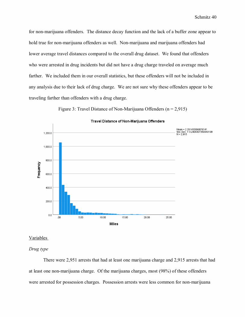
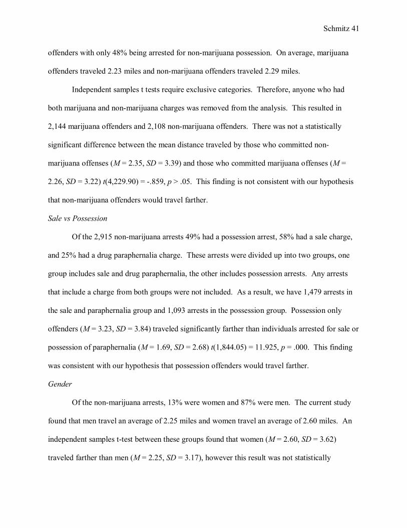
When only looking at non-marijuana offenses, the average travel distance decreased
slightly to 2.29 miles. The farthest an individual traveled was 23 miles and fifty percent of
offenders traveled 1.19 miles or less. Of the 2,915 arrests for non-marijuana offenses, 17% had
the same incident and home location. Figure 3 below illustrates the travel distance distribution
Schmitz 40
for non-marijuana offenders. The distance decay function and the lack of a buffer zone appear to
hold true for non-marijuana offenders as well. Non-marijuana and marijuana offenders had
lower average travel distances compared to the overall drug dataset. We found that offenders
who were arrested in drug incidents but did not have a drug charge traveled on average much
farther. We included them in our overall statistics, but these offenders will not be included in
any analysis due to their lack of drug charge. We are not sure why these offenders appear to be
traveling farther than offenders with a drug charge.
Figure 3: Travel Distance of Non-Marijuana Offenders (n = 2,915)
Variables
Drug type
There were 2,951 arrests that had at least one marijuana charge and 2,915 arrests that had
at least one non-marijuana charge. Of the marijuana charges, most (98%) of these offenders
were arrested for possession charges. Possession arrests were less common for non-marijuana
Schmitz 41
offenders with only 48% being arrested for non-marijuana possession. On average, marijuana
offenders traveled 2.23 miles and non-marijuana offenders traveled 2.29 miles.
Independent samples t tests require exclusive categories. Therefore, anyone who had
both marijuana and non-marijuana charges was removed from the analysis. This resulted in
2,144 marijuana offenders and 2,108 non-marijuana offenders. There was not a statistically
significant difference between the mean distance traveled by those who committed non-
marijuana offenses (M = 2.35, SD = 3.39) and those who committed marijuana offenses (M =
2.26, SD = 3.22) t(4,229.90) = -.859, p > .05. This finding is not consistent with our hypothesis
that non-marijuana offenders would travel farther.
Sale vs Possession
Of the 2,915 non-marijuana arrests 49% had a possession arrest, 58% had a sale charge,
and 25% had a drug paraphernalia charge. These arrests were divided up into two groups, one
group includes sale and drug paraphernalia, the other includes possession arrests. Any arrests
that include a charge from both groups were not included. As a result, we have 1,479 arrests in
the sale and paraphernalia group and 1,093 arrests in the possession group. Possession only
offenders (M = 3.23, SD = 3.84) traveled significantly farther than individuals arrested for sale or
possession of paraphernalia (M = 1.69, SD = 2.68) t(1,844.05) = 11.925, p = .000. This finding
was consistent with our hypothesis that possession offenders would travel farther.
Gender
Of the non-marijuana arrests, 13% were women and 87% were men. The current study
found that men travel an average of 2.25 miles and women travel an average of 2.60 miles. An
independent samples t-test between these groups found that women (M = 2.60, SD = 3.62)
traveled farther than men (M = 2.25, SD = 3.17), however this result was not statistically
Schmitz 42
significant t(456.816) = -1.797, p = 0.073. This finding does not support our hypothesis that
women would travel shorter distances.
Race and ethnicity
Fifteen percent of the non-marijuana arrests were white offenders, 21% were Latino
offenders, and 64% were Black offenders. There were 9 Asian offenders and 2 offenders who
did not have race and ethnicity listed and were removed from the analysis. A one way ANOVA
found that travel distance varies significantly by race and ethnicity F(2, 903) = 166.42, p=.000.
Tukey’s post hoc procedure indicated that Latino offenders (M = 1.64, SD =2.66) and Black
offenders (M = 1.93, SD =2.74) traveled significantly less for non-marijuana offenses compared
to white offenders (M = 4.76, SD =4.57). There was not a significant difference between black
and Latino offenders. This finding partially supports our hypothesis.
Age
Figure 3 illustrates the distribution of offenders by age. The number of offenders by age
peaks around the late twenties before decreasing sharply. The average age of non-marijuana
offenders was 31 years old. The youngest offender was 14 at the time of the offense and the
oldest offender was 75. The correlation between travel distance and age at offense can be seen in
scatter plot below (figure 4). As expected, based on the figure, there was not a significant
correlation between travel distance and age. An independent samples t-test was also used to
determine whether there were significant differences in travel distance for juvenile offenders.
This test found that there were no significant differences in travel distances between those 26 and
older (M = 2.29, SD = 3.25) and those younger than 26 (M = 2.30, SD = 3.23) t(2,102.063) = -
.122, p = 0.903. Both of these findings did not support our hypothesis that juvenile offenders
would travel shorter distances.
Schmitz 44
Figure 4: Scatter Plot of Miles by Age (n = 2,915)
Co-offenders
Most individuals offended by themselves, only one third of offenders were arrested with
at least one other individual. Possession and sale offenders had a different likelihood of having a
co-offender. Of the sale offenders, about 40% had a co-offender and about 24% of possession
offenders had a co-offender charge. An independent samples t-test found there was a significant
difference in travel distance between those with a co-offender and those without. Individuals
without a co-offender (M = 2.42, SD = 3.37) traveled significantly farther than those who had a
co-offender (M = 2.05, SD = 2.97) t(2,306.365) = 3.032, p = 0.002. This finding did not support
our hypothesis that co-offenders would travel farther.
Repeat Offenders
Over two thirds of non-marijuana offenders (70%) were arrested for more than one crime
Schmitz 45
during the time period of the study. For some of these offenders, the crime was another drug
crime, however some were arrested for other crime types. Those who had more than one arrest
in the dataset (M = 2.03, SD = 2.92) traveled significantly shorter distances than those arrested
only once during the time period (M = 2.88, SD = 3.81) t(1,361.664) = 5.871, p = 0.000. This
finding was not confident with our hypothesis that repeat offenders would travel farther.
Project Area
The Project Area located in Northeast Rochester is the site of many non-marijuana
arrests. Within the dataset used for this analysis 449 (15.4%) of the arrests were located within
the Project Area. When comparing offender travel distance for incidents in and out of the
Project Area, those with incidents in the Project Area (M = 2.03, SD = 2.92) traveled
significantly shorter distances than those with incidents outside of the Project Area (M = 2.88,
SD = 3.81) t(1,361.664) = 5.871, p = 0.000. These results were not consistent with our
hypothesis that Project Area offenders would travel farther.
Discussion
Overall, this analysis resulted in many unexpected findings. Based on previous research
we expected to find that marijuana offenders would travel significantly shorter distances
compared to offenders arrested for a drug other than marijuana (Johnson, Taylor, & Ratcliffe,
2013). When looking at the average distance traveled for both groups, non-marijuana offenders
traveled slightly farther, however this difference was not statistically significant. Previous
research has only investigated differences between buyers of marijuana and other drugs. It is
possible that including sellers in our analysis for both groups resulted in the lack of differences
between the groups. Sellers and buyers are distinctly different groups and the different
distributions of these groups between marijuana and non-marijuana offenders may have affected
Schmitz 46
the analysis. About 50% of non-marijuana offenders had a possession charge compared to
marijuana offenders where over 98% were arrested for possession. Previous research has found
that buyers travel longer distances than sellers (Johnson, 2016), if we only included buyers in
this analysis, then we may have found evidence to support previous research.
Expected differences between the groups was part of the reason we did not include
marijuana offenders in the rest of our analysis. However, even though we did not find those
differences, the decriminalization of marijuana in New York and the differences between
marijuana and other drugs supports our decision to keep these separate. Our analysis is
interested in travel patterns of non-marijuana offenders so including marijuana offenders would
have changed the focus of the study
Consistent with prior research (i.e., Johnson, 2016) we found that individuals who
purchased non-marijuana drugs traveled farther than individuals who were arrested for sale of
non-marijuana. This difference may be due to the different motives of drug sellers and buyers.
Drug sellers are likely going to want to stay relatively close to their house to reduce the costs of
offending and possibly due to being known for a specific location. Drug sellers also have the
power to determine where they sell, while drug buyers have to go to where the product is sold.
Buyers have a bit more freedom to choose where to offend and are likely going to make some
buying decisions while under the influence which may lead to traveling further. If buyers hear of
good drugs, they may be willing to travel farther to a location or if they are desperate for drugs,
they may be willing to travel farther to get to a location.
Unlike Johnson (2016), the current analysis used New York State Penal Law instead of
the UCR categorization. We utilized Penal Law over UCR code as the MCAC analyst stated this
was not reliable in the dataset. By using Penal Law, we were able to include individuals arrested
Schmitz 47
for possession of paraphernalia which would not be included under sale by using UCR codes.
Based on the Penal Law, we found that offenders arrested for paraphernalia are typically selling
drugs, therefore including them in the seller category allows for a more accurate representation
of drug sellers.
Partially consistent with prior research, we found that white offenders traveled
significantly farther than Latino and Black offenders. Unlike previous studies, we did not find
that Latino offenders traveled significantly shorter distances compared to Black and white
offenders (Johnson, Taylor, & Ratcliffe, 2013). Studies that previously investigated race were
able to differentiate between different drugs and found that Latino offenders traveled shorter
distances to purchase heroin specifically. As the current study focuses on an area with a heroin
market, we expected that many offenders would have been arrested for heroin and Latino
offenders would travel shorter distances. Our data was not able to distinguish between different
drugs beyond marijuana and other. It is possible that the ability to further refine our data by drug
type would have identified these differences.
The differences between white offenders and non-white offenders could also be a result
of the makeup of the city and suburbs. Areas closer to the open-air heroin market have higher
rates of minorities compared to areas farther away. Therefore, non-white offenders have more
opportunities to purchase drugs closer to their home compared to white offenders. Previous
research has also found that officers police Black neighborhoods differently than they police
white neighborhoods (Gaston, 2019). This could produce further bias in the data and
overrepresent Black drug offenders. Differences found by race could be a result of this bias in
enforcement.
Unlike previous studies that found repeat offenders traveled farther, the current study
Schmitz 48
found that repeat offenders traveled significantly shorter distances (Levine & Lee, 2013). There
are several possible reasons for this finding. One possibility for this difference is that there are
not as many places to purchase drugs in Rochester compared to other communities so those that
offend are not able to find a new place farther from their home. Sellers are also not able to travel
to new locations since there is only one drug market in the area. It is also possible that repeat
offenders are individuals known to law enforcement, so in an effort to reduce their exposure to
law enforcement, they stay closer to their home.
In the current study we found that individuals with a co-offender traveled shorter
distances compared to those who offended alone. Previous studies investigating the effect of co-
offenders found that individuals arrested for drug sales traveled farther distances if they had a co-
offender (Levine & Lee, 2013). We initially thought the difference in results could possibly be
due to the inclusion of possession offenders in our analysis and that individuals arrested for
possession with a co-offender may travel shorter distances. However, about 70% of individuals
with a co-offender were arrested for sale and not possession. One possible explanation for why
offenders travel shorter distances with a co-offender is that they may not actually be offending
with them. It could possibly be an individual purchasing drugs from another individual and they
both traveled somewhere relatively close to their house. Another possibility is that sellers are
typically traveling less far and since there are more of them that have co-offenders this may skew
the data. Future research is needed to determine more about why this finding occurred in our
data but not in previous research.
The current study found that individuals who offended within the Project Area, which is
the site of an open-air heroin market, traveled shorter distances. We had expected to find that
individuals would travel farther to get to these locations based on previous work about deprived
Schmitz 49
areas (Forsyth et al., 1992). One possible explanation for this is that individuals who live close
to the Project Area are able to acquire drugs more often than those who live farther away.
Individuals who live far away may only come into the area once a week compared to those who
live there could purchase drugs every day. The frequency of trips could result in offenders living
close by being arrested more often and skewing the results. Individuals over time may also
move to be closer to the Project Area if they are repeatedly using drugs.
There were no significant differences in travel distance for male and female offenders, we
had expected that men would travel farther. We did have a very small sample of women which
also could have impacted our results. Previous studies on drug offenders for both sale and
possession have found that men travel farther (Pettiway, 1995; Levine & Lee, 2013), however
some studies have found that this effect is only for cocaine and there is no significant difference
for heroin arrests (Johnson, Taylor, & Ratcliffe, 2013). All these studies used different methods
and populations therefore it can be difficult to compare across studies. More studies are needed
to determine the effects of gender on the drug JTC.
Like gender there were previous mixed findings on the effects of age on the JTC. The
broader JTC field has found that juveniles travel shorter distances (Levine & Lee, 2013), yet the
one study on JTC for drug offenders did not find a difference (Johnson, Taylor, & Ratcliffe,
2013). We expected to find that juvenile offenders would not travel as far as older offenders,
however there were no significant differences between the groups. To test age differences, we
used both a correlation and independent samples t-test. While juvenile offenders are typically
individuals under 18, the current sample did not have a large enough sample under 18 to be used.
As a result, we used individuals under 26 and, like Johnson, Taylor, and Ratcliffe (2013), they
also did not find a difference with age. Levine and Lee (2013) had a large enough sample under
Schmitz 50
18 for all offender types and did find juvenile offenders traveled shorter distances. Levine and
Lee (2013) did test an interaction between gender and age specifically for drug seller arrests.
Both of these studies found that there is an interaction between age and gender with male
juvenile offenders traveling significantly shorter distances (Johnson, Taylor, & Ratcliffe, 2013;
Levine & Lee, 2013). Offenders under 18 are likely very different than those 18 to 26 due to
access to resources. Individuals under 18 may not be old enough to drive or have access to a car.
Those under 18 may be limited to locations where they can walk too. It is quite possible that
there are age differences in travel distance that we are unable to test based on the nature of the
current sample.
Limitations
One limitation with this study is the data we have available. Data from police
departments is biased as not every offender is equally likely to be arrested and a few studies have
found there are disparities in policing in different neighborhoods (Gaston, 2019). Based on our
own experience with observations and interviews with law enforcement, we know that the police
do not make arrests for every drug offense, as that would be impossible. If arrests are not an
accurate random sample of all offenders in an area, then the results may not reflect the true travel
patterns of offenders. There are several findings in the study that may be a result of biased
policing. There are not many other sources available besides policing data to analyze this aspect
of offending, however we recognize that policing behavior in certain neighborhoods may cause
findings that do not align with reality. Though conducting qualitative studies similar to Forsyth
et al. (1992) and Pettiway (1995) could help to address this limitation.
Another limitation that may have affected our results is the strict inclusion criteria for this
study. An arrest incident could only be included if it had coordinates for the home and incident
Schmitz 51
address. Over 2,000 incidents could not be included in the study due to this requirement. In
addition, besides the address not having coordinates, the incident location may not necessarily
represent where the individual traveled to purchase or sell drugs. It is possible that officers will
arrest individuals for some other charge and in the process find drugs on them. They will likely
use the location of the incident they initially responded to or witnessed and not the location of
the purchase or sale of drugs. In the dataset we have also found that incident locations are often
listed at the Public Safety Building or other law enforcement agencies throughout Rochester.
These locations may not reflect the actual drug buying incident and just at what point the drug
was discovered by an officer or probation officer.
Lastly, the group of interest in this study was non-marijuana offenders yet this may not
have been the best group to analyze. Our results differed somewhat from other scholarship in
this area. The inclusion of both drug sellers and buyers may have caused many of our results to
not reflect previous work and therefore limits the generalizability of our results. Buyers and
sellers have different motivations and goals, and their behavior may not be the same. They are
likely different types of offenders with different motivations. Had we separated these groups into
two different samples and repeated these tests we may find different results.
Future Research
As noted in our limitation section, conducting a future study that considers buyers and
sellers as two separate offender types may provide us with results that more accurately reflect
what is happening on the ground in communities. These offenders are likely two distinct groups
that have different motivations. As a result, any findings from the current study may reflect this
combination and not differing behavior in Rochester. To increase the generalizability of our
results and our ability to compare this research to previous studies, we intend to repeat the
Schmitz 52
current analysis dividing by sellers and buyers. This paper will test all of the same hypotheses
for each group separately. We hope that this change will allow us to further add to the JTC field
for drug offenders. Another possible study we could complete would involve interviewing
offenders about these results and see if they can provide further insight into these findings. In
addition, we could complete a study that would involve looking at distance traveled by offenders
in an area similar to Rochester.
Schmitz 53
References
Ackerman, J. M., & Rossmo, D. K. (2015). How far to travel? A multilevel analysis of the
residence-to-crime distance. Journal of Quantitative Criminology, 31(2), 237-262.
Altheimer, I., Duda-Banwar, J., & Klofas, J. (2018). A neighborhood's struggle with opioids:
Our window to the national opioid crisis.
Barnum, J. D., Campbell, W. L., Trocchio, S., Caplan, J. M., & Kennedy, L. W. (2017).
Examining the environmental characteristics of drug dealing locations. Crime &
Delinquency, 63(13), 1731-1756.
Block, R., & Bernasco, W. (2009). Finding a serial burglar's home using distance decay and
conditional origin–destination patterns: a test of empirical Bayes journey‐to‐crime
estimation in the Hague. Journal of Investigative Psychology and Offender
Profiling, 6(3), 187-211.
Bernasco, W. (2010). A sentimental journey to crime: Effects of residential history on crime
location choice. Criminology, 48(2), 389-416.
Bernasco, W., & van Dijke, R. (2020). Do offenders avoid offending near home? A systematic
review of the buffer zone hypothesis. Crime Science, 9, 1-10.
Brantingham, P. J., & Brantingham, P. L. (Eds.). (1981). Environmental criminology (pp. 27-54).
Beverly Hills, CA: Sage Publications.
Brantingham, P. J., & Brantingham, P. L. (1984). Patterns in crime. New York: Macmillan.
Cozens, P. M., Saville, G., & Hillier, D. (2005). Crime prevention through environmental design
(CPTED): a review and modern bibliography. Property management.
de Jong, E., Bernasco, W., & Lammers, M. (2019). Situational correlates of adolescent substance
use: An improved test of the routine activity theory of deviant behavior. Journal of
Schmitz 54
Quantitative Criminology, 1-28.
Forsyth, A. J., Hammersley, R. H., Lavelle, T. L., & Murray, K. J. (1992). Geographical aspects
of scoring illegal drugs. The British Journal of Criminology, 32(3), 292-309.
Gaston, S. (2019). Producing race disparities: A study of drug arrests across place and race.
Criminology, 57(3), 424-451.
Harocopos, A., & Hough, M. (2005). Center for Problem-Oriented Policing. Retrieved from
https://popcenter.asu.edu/content/drug-dealing-open-air-markets-0
Iwanski, N., Frank, R., Dabbaghian, V., Reid, A., & Brantingham, P. (2011, September).
Analyzing an offender's journey to crime: A criminal movement model (crimm). In 2011
European intelligence and security informatics conference (pp. 70-77). IEEE.
Johnson, L. T. (2016). Drug markets, travel distance, and violence: Testing a typology. Crime &
Delinquency, 62(11), 1465-1487.
Johnson, L. T., Taylor, R. B., & Ratcliffe, J. H. (2013). Need drugs, will travel?: The distances to
crime of illegal drug buyers. Journal of Criminal Justice, 41(3), 178-187.
Johnston-McCabe, P., Levi-Minzi, M., Van Hasselt, V. B., & Vanderbeek, A. (2011). Domestic
violence and social support in a clinical sample of deaf and hard of hearing women.
Journal of Family Violence, 26(1), 63-69.
Knutsson, J. (1997). Restoring public order in a city park. Policing for prevention: Reducing
crime, public intoxication and injury, 7, 133-151.
Levine, N., & Lee, P. (2013). Journey-to-crime by gender and age group in Manchester,
England. In Crime modeling and mapping using geospatial technologies (pp. 145-178).
Schmitz 55
Springer, Dordrecht.
Levy, J. M., Irvin-Erickson, Y., & La Vigne, N. (2018). A case study of bicycle theft on the
Washington DC Metrorail system using a Routine Activities and Crime Pattern theory
framework. Security Journal, 31(1), 226-246.
Miller, J. (2013). Individual offending, routine activities, and activity settings: Revisiting the
routine activity theory of general deviance. Journal of Research in Crime and
Delinquency, 50(3), 390-416.
Mustaine, E. E., & Tewksbury, R. (1999). A routine activity theory explanation for women's
stalking victimizations. Violence Against Women, 5(1), 43-62.
Pettiway, L. E. (1995). Copping crack: The travel behavior of crack users. Justice Quarterly,
12(3), 499-524.
Santtila, P., Laukkanen, M., & Zappalà, A. (2007). Crime behaviours and distance travelled in
homicides and rapes. Journal of Investigative Psychology and Offender Profiling, 4(1), 1-
15.
Townsley, M., & Sidebottom, A. (2010). All offenders are equal, but some are more equal than
others: Variation in journeys to crime between offenders. Criminology, 48(3), 897-917.
Van Koppen, P. J., & De Keijser, J. W. (1997). Desisting distance decay: On the aggregation of
individual crime trips. Criminology, 35(3), 505-515.
White, R. C. (1932). The relation of felonies to environmental factors in Indianapolis. Social
Forces, 10(4), 498-509.
Wortley, R., & Townsley, M. (Eds.). (2016). Environmental criminology and crime analysis.
Taylor & Francis.
Schmitz 56
Appendix A
Category Included Penal Codes
Non-Marijuana Possession PL 220.03 - .21 excluding 220.06 04 and 220.16
Non-Marijuana Paraphernalia PL 220.50 - .72
Non-Marijuana Sale/Intent to Sell PL 220.16 and 220.31 - .44
Marijuana Sale PL 221.35 - .55
Marijuana Possession PL 221.05 - .30 and 220.06 04
DUI Drugs VTL 1192 - 4 of 4A