Received: 5 July 2013 – Published in Hydrol. Earth Syst. Sci. Discuss.: 19 July 2013Revised: 15 November 2013 – Accepted: 5 December 2013 – Published: 20 December 2013
Abstract. The June 2013 flood in the Upper Danube Basinwas one of the largest floods in the past two centuries. Anatmospheric blocking situation produced precipitation ex-ceeding 300 mm over four days at the northern rim of theAlps. The high precipitation, along with high antecedent soilmoisture, gave rise to extreme flood discharges in a numberof tributaries including the Tiroler Ache, Saalach, Salzachand Inn. Runoff coefficients ranged from 0.2 in the Bavar-ian lowlands to 0.6 in the Alpine areas in Austria. Snow-fall at high altitudes (above about 1600 m a.s.l.) reduced therunoff volume produced. Precipitation was distributed overtwo blocks separated by a few hours, which resulted in a sin-gle peak, long-duration flood wave at the Inn and Danube.At the confluence of the Bavarian Danube and the Inn, thesmall time lag between the two flood waves exacerbated thedownstream flood at the Danube. Because of the long dura-tion and less inundation, there was less flood peak attenu-ation along the Austrian Danube reach than for the August2002 flood. Maximum flood discharges of the Danube at Vi-enna were about 11 000 m3 s−1, as compared to 10 300, 9600and 10 500 m3 s−1 in 2002, 1954 and 1899, respectively. Thispaper reviews the meteorological and hydrological charac-teristics of the event as compared to the 2002, 1954 and1899 floods, and discusses the implications for hydrologicalresearch and flood risk management.
1 Introduction
In June 2013 a major flood struck the Upper Danube Basincausing heavy damage along the Danube and numerous trib-utaries. The city centre of Passau (at the confluence of theDanube, Inn and Ilz) experienced flood levels that were simi-lar to the highest recorded flood in 1501. Extraordinary flood
discharges were recorded along the Saalach and Tiroler Acheat the Austrian–Bavarian border. The flood discharge of theDanube at Vienna exceeded those observed in the past twocenturies.
The June 2013 flood comes at a time with an amazinghistory of recent large floods. In August 2005, the Danubetributaries in western Tyrol and the south of Bavaria wereflooded through extensive precipitation and high antecedentsoil moisture (BLU, 2006). In August 2002, a major floodhit the entire Upper Danube Basin. Damage was most se-vere at the northern tributaries of the Austrian Danube at theCzech border, in particular the Aist and Kamp rivers. At theKamp, flood discharges were almost three times the largestflood in the century before (Gutknecht et al., 2002). Flood-ing was extensive along the entire Austrian Danube whichresulted in the use of the term “century flood”. The precedingdecades were relatively flood-poor at the Danube aside frommore minor floods in 1991, 1966 and 1965; however a verylarge flood occurred in July 1954 with major damage alongthe entire Upper Danube. Again, a couple of decades withalmost no floods preceded. The flood of September 1899,then, was the largest measured flood along the Danube with48 h precipitation totals exceeding 200 mm over an area of1000 km2 (Kresser, 1957). Major floods occurred in August1897, February 1862 and October 1787 with a long record ofprevious events (Kresser, 1957; Pekarová et al., 2013).
The aim of this paper is to analyse the causal factors of theJune 2013 flood including the atmospheric situation, runoffgeneration and the propagation of the flood wave along theDanube and tributaries. Given the extraordinary nature ofthe 2013 flood, the paper also compares this flood with thelargest Upper Danube floods in the past two centuries, i.e.the floods in August 2002, July 1954 and September 1899.
Published by Copernicus Publications on behalf of the European Geosciences Union.
5198 G. Blöschl et al.: The June 2013 flood in the Upper Danube Basin
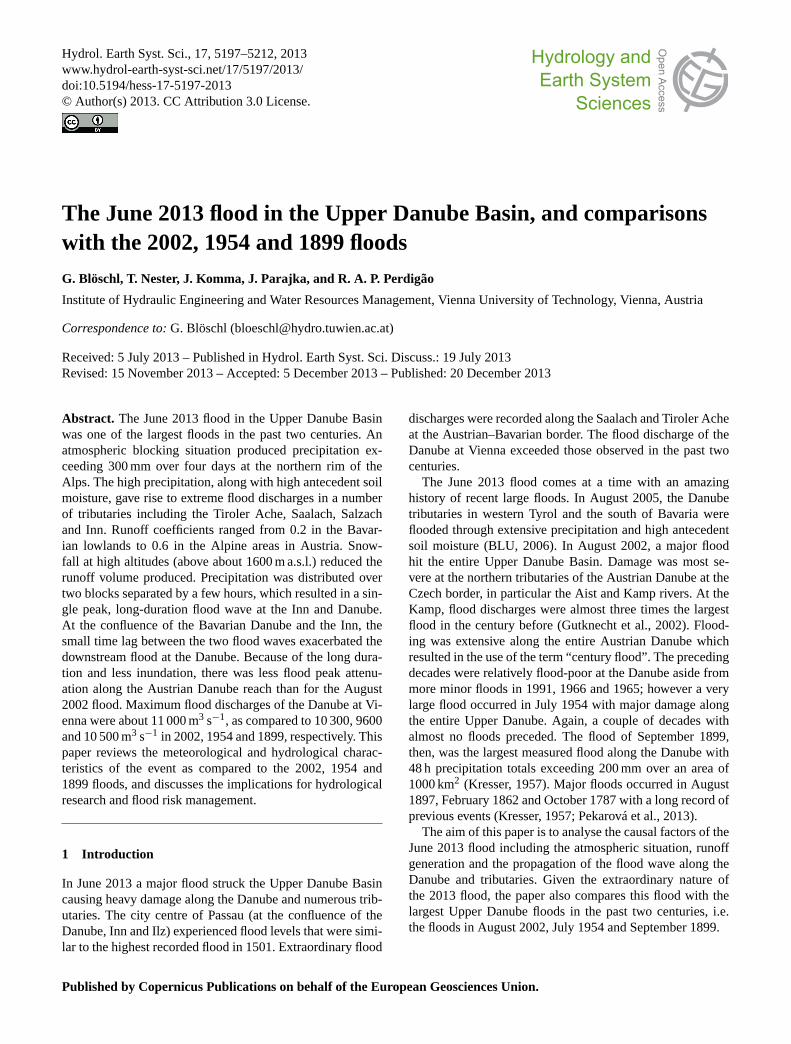
Fig. 1. The Upper Danube Basin upstream of Wildungsmauer. Red circles indicate stream gauges used in this paper. Black circles indicatethe cities of Vienna and Passau. For catchment areas and mean elevations of the catchments see Appendix A.
2 The Upper Danube Basin
The Upper Danube Basin consists of two main subcatch-ments, the Bavarian Danube and the Inn. The BavarianDanube catchment in the northwest comprises lowlands withdiverse geology. Quaternary and Tertiary deposits prevail,which are highly permeable and provide large subsurfacestorage in porous aquifers, and there is also karst in thenorthwest. Some of the tributaries, such as the Lech andIsar, originate from the Alps. Elevations range from 310 to3000 m a.s.l. Mean annual precipitation ranges from 650 tomore than 2000 mm yr−1, resulting in mean annual runoffdepths from 100 to 1500 mm yr−1 (BMU, 2003). The Inncatchment, further in the south, drains a large part of theAustrian Alps. An important tributary is the Salzach. Ge-ologically, the Inn catchment mainly consists of the north-ern Calcareous Alps, the Palaeozoic Greywacke zone fur-ther in the south and the Crystalline zone along the ridge ofthe eastern Alps (Janoschek and Matura, 1980). Elevationsrange from 310 to 3800 m. Mean annual precipitation rangesfrom 600 to more than 2000 mm yr−1, resulting in mean an-nual runoff depths from 100 to 1600 mm yr−1 (Parajka et al.,2007; Nester et al., 2011).
The Bavarian Danube and the Inn join at Passau. Down-stream of the confluence, along the Austrian reach of theDanube, southern tributaries from the high rainfall areas inthe Calcareous Alps include the Traun, Enns and Ybbs. Thenorthern tributaries from the lower rainfall areas with mainly
granitic geology include the Aist and Kamp. Flood protectionlevees have been built along many tributaries and the Danubeitself during the 19th and 20th century. The total catchmentarea of the Danube at Wildungsmauer downstream of Viennais 104 000 km2. Figure 1 shows the catchments discussed inthis paper, and Appendix A gives their main characteristics.
3 Large-scale atmospheric conditions
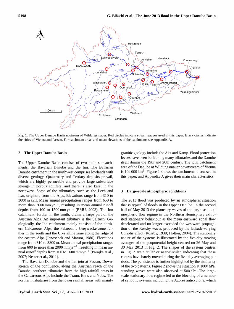
The 2013 flood was produced by an atmospheric situationthat is typical of floods in the Upper Danube. In the secondhalf of May 2013 the planetary waves of the large-scale at-mospheric flow regime in the Northern Hemisphere exhib-ited stationary behaviour as the mean eastward zonal flowdecelerated and no longer exceeded the westward propaga-tion of the Rossby waves produced by the latitude-varyingCoriolis effect (Rossby, 1939; Holton, 2004). The stationarynature of the systems is illustrated by the five-day movingaverages of the geopotential height centred on 26 May and30 May 2013 in Fig. 2. The shapes of the system centresin Fig. 2 are circular or near-circular, indicating that thesecentres have barely moved during the five-day averaging pe-riods. The persistence is further highlighted by the similarityof the two patterns. Figure 2 shows the situation at 1000 hPa;standing waves were also observed at 500 hPa. The large-scale stationary flow regime led to the blocking of a numberof synoptic systems including the Azores anticyclone, which
G. Blöschl et al.: The June 2013 flood in the Upper Danube Basin 5199
Fig. 2. Geopotential height fields (in meter) at 1000 hPa of the Northern Hemisphere for latitudes above 20 degrees. Five-day movingaverages, centred on 26 May and 30 May 2013. The geopotential height difference between consecutive isolines is 15 m. Based on theNCEP-NCAR Reanalysis data sets (Kistler et al., 2001).
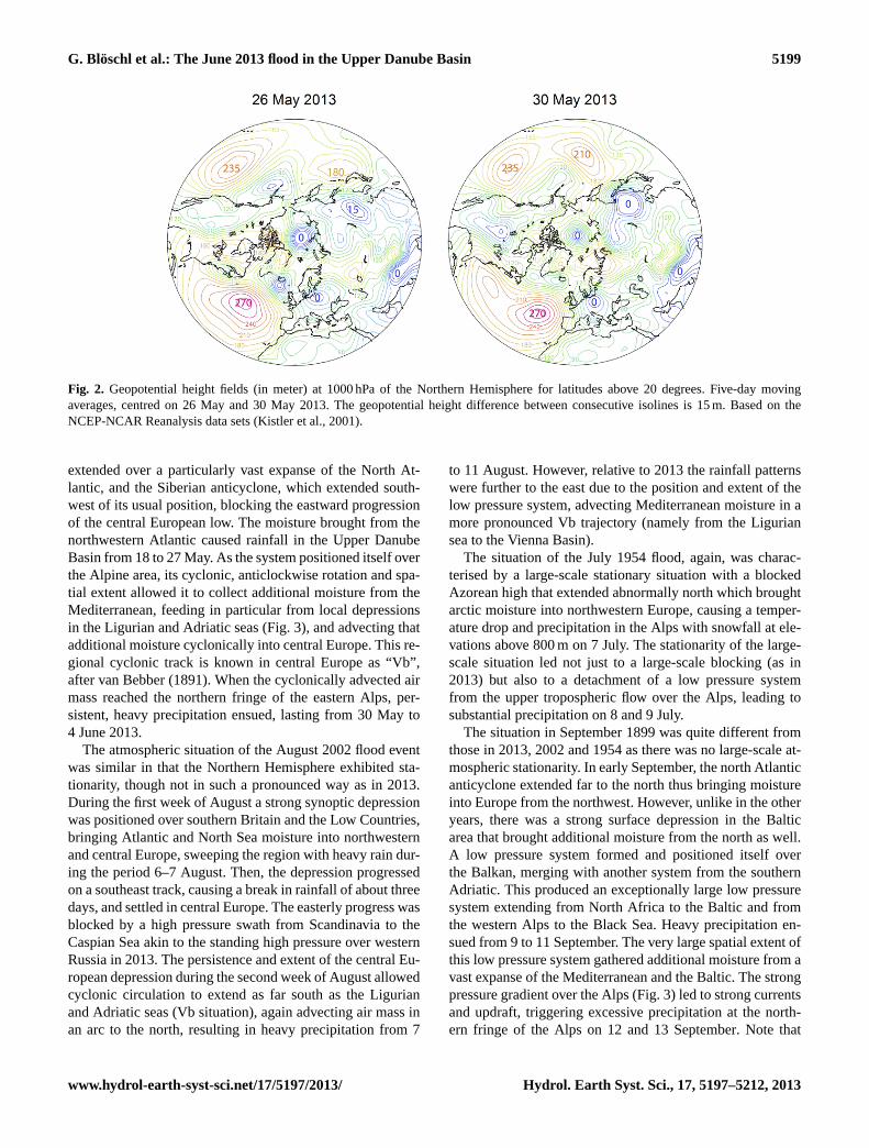
extended over a particularly vast expanse of the North At-lantic, and the Siberian anticyclone, which extended south-west of its usual position, blocking the eastward progressionof the central European low. The moisture brought from thenorthwestern Atlantic caused rainfall in the Upper DanubeBasin from 18 to 27 May. As the system positioned itself overthe Alpine area, its cyclonic, anticlockwise rotation and spa-tial extent allowed it to collect additional moisture from theMediterranean, feeding in particular from local depressionsin the Ligurian and Adriatic seas (Fig. 3), and advecting thatadditional moisture cyclonically into central Europe. This re-gional cyclonic track is known in central Europe as “Vb”,after van Bebber (1891). When the cyclonically advected airmass reached the northern fringe of the eastern Alps, per-sistent, heavy precipitation ensued, lasting from 30 May to4 June 2013.
The atmospheric situation of the August 2002 flood eventwas similar in that the Northern Hemisphere exhibited sta-tionarity, though not in such a pronounced way as in 2013.During the first week of August a strong synoptic depressionwas positioned over southern Britain and the Low Countries,bringing Atlantic and North Sea moisture into northwesternand central Europe, sweeping the region with heavy rain dur-ing the period 6–7 August. Then, the depression progressedon a southeast track, causing a break in rainfall of about threedays, and settled in central Europe. The easterly progress wasblocked by a high pressure swath from Scandinavia to theCaspian Sea akin to the standing high pressure over westernRussia in 2013. The persistence and extent of the central Eu-ropean depression during the second week of August allowedcyclonic circulation to extend as far south as the Ligurianand Adriatic seas (Vb situation), again advecting air mass inan arc to the north, resulting in heavy precipitation from 7
to 11 August. However, relative to 2013 the rainfall patternswere further to the east due to the position and extent of thelow pressure system, advecting Mediterranean moisture in amore pronounced Vb trajectory (namely from the Liguriansea to the Vienna Basin).
The situation of the July 1954 flood, again, was charac-terised by a large-scale stationary situation with a blockedAzorean high that extended abnormally north which broughtarctic moisture into northwestern Europe, causing a temper-ature drop and precipitation in the Alps with snowfall at ele-vations above 800 m on 7 July. The stationarity of the large-scale situation led not just to a large-scale blocking (as in2013) but also to a detachment of a low pressure systemfrom the upper tropospheric flow over the Alps, leading tosubstantial precipitation on 8 and 9 July.
The situation in September 1899 was quite different fromthose in 2013, 2002 and 1954 as there was no large-scale at-mospheric stationarity. In early September, the north Atlanticanticyclone extended far to the north thus bringing moistureinto Europe from the northwest. However, unlike in the otheryears, there was a strong surface depression in the Balticarea that brought additional moisture from the north as well.A low pressure system formed and positioned itself overthe Balkan, merging with another system from the southernAdriatic. This produced an exceptionally large low pressuresystem extending from North Africa to the Baltic and fromthe western Alps to the Black Sea. Heavy precipitation en-sued from 9 to 11 September. The very large spatial extent ofthis low pressure system gathered additional moisture from avast expanse of the Mediterranean and the Baltic. The strongpressure gradient over the Alps (Fig. 3) led to strong currentsand updraft, triggering excessive precipitation at the north-ern fringe of the Alps on 12 and 13 September. Note that
5200 G. Blöschl et al.: The June 2013 flood in the Upper Danube Basin
Fig. 3. Sea level pressure (hPa) in central Europe on 31 May 2013(00:00), 10 August 2002 (12:00), 8 July 1954 (00:00), 13 September1899 (06:00) (all times in UTC). 2013, 2002 and 1954 are based onthe NCEP-NCAR Reanalysis, while 1899 is from Lauda (1900).Circles indicate location of Passau. Times have been chosen as tobe most relevant for the precipitation production.
the pressure map of Lauda (1900) is based on more than 100stations in Europe, so it shows considerable spatial detail.
4 Local meteorological conditions (precipitationand snow)
4.1 Regional precipitation patterns of the 2013 flood
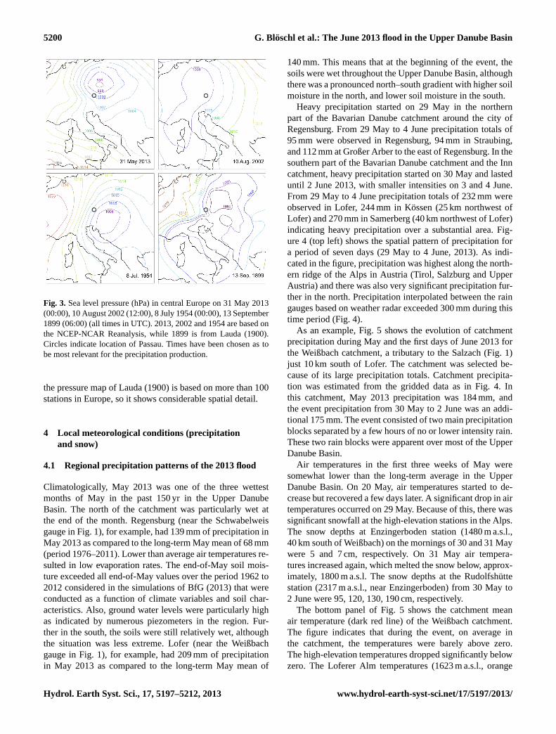
Climatologically, May 2013 was one of the three wettestmonths of May in the past 150 yr in the Upper DanubeBasin. The north of the catchment was particularly wet atthe end of the month. Regensburg (near the Schwabelweisgauge in Fig. 1), for example, had 139 mm of precipitation inMay 2013 as compared to the long-term May mean of 68 mm(period 1976–2011). Lower than average air temperatures re-sulted in low evaporation rates. The end-of-May soil mois-ture exceeded all end-of-May values over the period 1962 to2012 considered in the simulations of BfG (2013) that wereconducted as a function of climate variables and soil char-acteristics. Also, ground water levels were particularly highas indicated by numerous piezometers in the region. Fur-ther in the south, the soils were still relatively wet, althoughthe situation was less extreme. Lofer (near the Weißbachgauge in Fig. 1), for example, had 209 mm of precipitationin May 2013 as compared to the long-term May mean of
140 mm. This means that at the beginning of the event, thesoils were wet throughout the Upper Danube Basin, althoughthere was a pronounced north–south gradient with higher soilmoisture in the north, and lower soil moisture in the south.
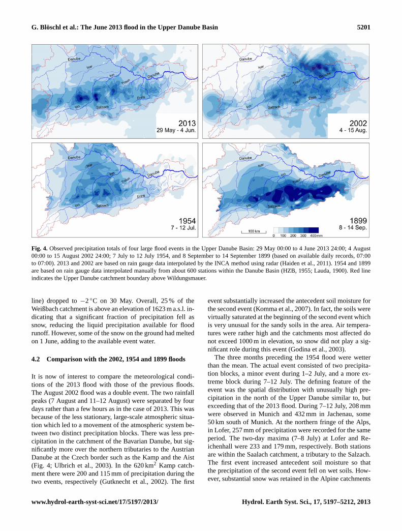
Heavy precipitation started on 29 May in the northernpart of the Bavarian Danube catchment around the city ofRegensburg. From 29 May to 4 June precipitation totals of95 mm were observed in Regensburg, 94 mm in Straubing,and 112 mm at Großer Arber to the east of Regensburg. In thesouthern part of the Bavarian Danube catchment and the Inncatchment, heavy precipitation started on 30 May and lasteduntil 2 June 2013, with smaller intensities on 3 and 4 June.From 29 May to 4 June precipitation totals of 232 mm wereobserved in Lofer, 244 mm in Kössen (25 km northwest ofLofer) and 270 mm in Samerberg (40 km northwest of Lofer)indicating heavy precipitation over a substantial area. Fig-ure 4 (top left) shows the spatial pattern of precipitation fora period of seven days (29 May to 4 June, 2013). As indi-cated in the figure, precipitation was highest along the north-ern ridge of the Alps in Austria (Tirol, Salzburg and UpperAustria) and there was also very significant precipitation fur-ther in the north. Precipitation interpolated between the raingauges based on weather radar exceeded 300 mm during thistime period (Fig. 4).
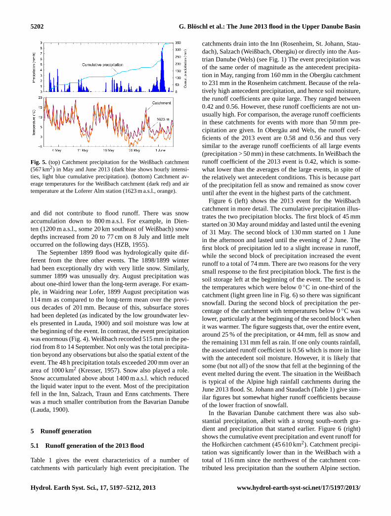
As an example, Fig. 5 shows the evolution of catchmentprecipitation during May and the first days of June 2013 forthe Weißbach catchment, a tributary to the Salzach (Fig. 1)just 10 km south of Lofer. The catchment was selected be-cause of its large precipitation totals. Catchment precipita-tion was estimated from the gridded data as in Fig. 4. Inthis catchment, May 2013 precipitation was 184 mm, andthe event precipitation from 30 May to 2 June was an addi-tional 175 mm. The event consisted of two main precipitationblocks separated by a few hours of no or lower intensity rain.These two rain blocks were apparent over most of the UpperDanube Basin.
Air temperatures in the first three weeks of May weresomewhat lower than the long-term average in the UpperDanube Basin. On 20 May, air temperatures started to de-crease but recovered a few days later. A significant drop in airtemperatures occurred on 29 May. Because of this, there wassignificant snowfall at the high-elevation stations in the Alps.The snow depths at Enzingerboden station (1480 m a.s.l.,40 km south of Weißbach) on the mornings of 30 and 31 Maywere 5 and 7 cm, respectively. On 31 May air tempera-tures increased again, which melted the snow below, approx-imately, 1800 m a.s.l. The snow depths at the Rudolfshüttestation (2317 m a.s.l., near Enzingerboden) from 30 May to2 June were 95, 120, 130, 190 cm, respectively.
The bottom panel of Fig. 5 shows the catchment meanair temperature (dark red line) of the Weißbach catchment.The figure indicates that during the event, on average inthe catchment, the temperatures were barely above zero.The high-elevation temperatures dropped significantly belowzero. The Loferer Alm temperatures (1623 m a.s.l., orange
G. Blöschl et al.: The June 2013 flood in the Upper Danube Basin 5201
Fig. 4. Observed precipitation totals of four large flood events in the Upper Danube Basin: 29 May 00:00 to 4 June 2013 24:00; 4 August00:00 to 15 August 2002 24:00; 7 July to 12 July 1954, and 8 September to 14 September 1899 (based on available daily records, 07:00to 07:00). 2013 and 2002 are based on rain gauge data interpolated by the INCA method using radar (Haiden et al., 2011). 1954 and 1899are based on rain gauge data interpolated manually from about 600 stations within the Danube Basin (HZB, 1955; Lauda, 1900). Red lineindicates the Upper Danube catchment boundary above Wildungsmauer.
line) dropped to−2◦C on 30 May. Overall, 25 % of theWeißbach catchment is above an elevation of 1623 m a.s.l. in-dicating that a significant fraction of precipitation fell assnow, reducing the liquid precipitation available for floodrunoff. However, some of the snow on the ground had meltedon 1 June, adding to the available event water.
4.2 Comparison with the 2002, 1954 and 1899 floods
It is now of interest to compare the meteorological condi-tions of the 2013 flood with those of the previous floods.The August 2002 flood was a double event. The two rainfallpeaks (7 August and 11–12 August) were separated by fourdays rather than a few hours as in the case of 2013. This wasbecause of the less stationary, large-scale atmospheric situa-tion which led to a movement of the atmospheric system be-tween two distinct precipitation blocks. There was less pre-cipitation in the catchment of the Bavarian Danube, but sig-nificantly more over the northern tributaries to the AustrianDanube at the Czech border such as the Kamp and the Aist(Fig. 4; Ulbrich et al., 2003). In the 620 km2 Kamp catch-ment there were 200 and 115 mm of precipitation during thetwo events, respectively (Gutknecht et al., 2002). The first
event substantially increased the antecedent soil moisture forthe second event (Komma et al., 2007). In fact, the soils werevirtually saturated at the beginning of the second event whichis very unusual for the sandy soils in the area. Air tempera-tures were rather high and the catchments most affected donot exceed 1000 m in elevation, so snow did not play a sig-nificant role during this event (Godina et al., 2003).
The three months preceding the 1954 flood were wetterthan the mean. The actual event consisted of two precipita-tion blocks, a minor event during 1–2 July, and a more ex-treme block during 7–12 July. The defining feature of theevent was the spatial distribution with unusually high pre-cipitation in the north of the Upper Danube similar to, butexceeding that of the 2013 flood. During 7–12 July, 208 mmwere observed in Munich and 432 mm in Jachenau, some50 km south of Munich. At the northern fringe of the Alps,in Lofer, 257 mm of precipitation were recorded for the sameperiod. The two-day maxima (7–8 July) at Lofer and Re-ichenhall were 233 and 179 mm, respectively. Both stationsare within the Saalach catchment, a tributary to the Salzach.The first event increased antecedent soil moisture so thatthe precipitation of the second event fell on wet soils. How-ever, substantial snow was retained in the Alpine catchments
5202 G. Blöschl et al.: The June 2013 flood in the Upper Danube Basin
Fig. 5. (top) Catchment precipitation for the Weißbach catchment(567 km2) in May and June 2013 (dark blue shows hourly intensi-ties, light blue cumulative precipitation). (bottom) Catchment av-erage temperatures for the Weißbach catchment (dark red) and airtemperature at the Loferer Alm station (1623 m a.s.l., orange).
and did not contribute to flood runoff. There was snowaccumulation down to 800 m a.s.l. For example, in Dien-ten (1200 m a.s.l., some 20 km southeast of Weißbach) snowdepths increased from 20 to 77 cm on 8 July and little meltoccurred on the following days (HZB, 1955).
The September 1899 flood was hydrologically quite dif-ferent from the three other events. The 1898/1899 winterhad been exceptionally dry with very little snow. Similarly,summer 1899 was unusually dry. August precipitation wasabout one-third lower than the long-term average. For exam-ple, in Waidring near Lofer, 1899 August precipitation was114 mm as compared to the long-term mean over the previ-ous decades of 201 mm. Because of this, subsurface storeshad been depleted (as indicated by the low groundwater lev-els presented in Lauda, 1900) and soil moisture was low atthe beginning of the event. In contrast, the event precipitationwas enormous (Fig. 4). Weißbach recorded 515 mm in the pe-riod from 8 to 14 September. Not only was the total precipita-tion beyond any observations but also the spatial extent of theevent. The 48 h precipitation totals exceeded 200 mm over anarea of 1000 km2 (Kresser, 1957). Snow also played a role.Snow accumulated above about 1400 m a.s.l. which reducedthe liquid water input to the event. Most of the precipitationfell in the Inn, Salzach, Traun and Enns catchments. Therewas a much smaller contribution from the Bavarian Danube(Lauda, 1900).
5 Runoff generation
5.1 Runoff generation of the 2013 flood
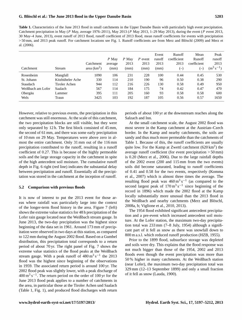
Table 1 gives the event characteristics of a number ofcatchments with particularly high event precipitation. The
catchments drain into the Inn (Rosenheim, St. Johann, Stau-dach), Salzach (Weißbach, Obergäu) or directly into the Aus-trian Danube (Wels) (see Fig. 1) The event precipitation wasof the same order of magnitude as the antecedent precipita-tion in May, ranging from 160 mm in the Obergäu catchmentto 231 mm in the Rosenheim catchment. Because of the rela-tively high antecedent precipitation, and hence soil moisture,the runoff coefficients are quite large. They ranged between0.42 and 0.56. However, these runoff coefficients are not un-usually high. For comparison, the average runoff coefficientsin these catchments for events with more than 50 mm pre-cipitation are given. In Obergäu and Wels, the runoff coef-ficients of the 2013 event are 0.58 and 0.56 and thus verysimilar to the average runoff coefficients of all large events(precipitation > 50 mm) in these catchments. In Weißbach therunoff coefficient of the 2013 event is 0.42, which is some-what lower than the averages of the large events, in spite ofthe relatively wet antecedent conditions. This is because partof the precipitation fell as snow and remained as snow coveruntil after the event in the highest parts of the catchment.
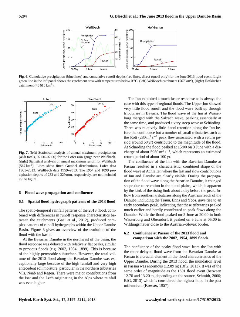
Figure 6 (left) shows the 2013 event for the Weißbachcatchment in more detail. The cumulative precipitation illus-trates the two precipitation blocks. The first block of 45 mmstarted on 30 May around midday and lasted until the eveningof 31 May. The second block of 130 mm started on 1 Junein the afternoon and lasted until the evening of 2 June. Thefirst block of precipitation led to a slight increase in runoff,while the second block of precipitation increased the eventrunoff to a total of 74 mm. There are two reasons for the verysmall response to the first precipitation block. The first is thesoil storage left at the beginning of the event. The second isthe temperatures which were below 0◦C in one-third of thecatchment (light green line in Fig. 6) so there was significantsnowfall. During the second block of precipitation the per-centage of the catchment with temperatures below 0◦C waslower, particularly at the beginning of the second block whenit was warmer. The figure suggests that, over the entire event,around 25 % of the precipitation, or 44 mm, fell as snow andthe remaining 131 mm fell as rain. If one only counts rainfall,the associated runoff coefficient is 0.56 which is more in linewith the antecedent soil moisture. However, it is likely thatsome (but not all) of the snow that fell at the beginning of theevent melted during the event. The situation in the Weißbachis typical of the Alpine high rainfall catchments during theJune 2013 flood. St. Johann and Staudach (Table 1) give sim-ilar figures but somewhat higher runoff coefficients becauseof the lower fraction of snowfall.
In the Bavarian Danube catchment there was also sub-stantial precipitation, albeit with a strong south–north gra-dient and precipitation that started earlier. Figure 6 (right)shows the cumulative event precipitation and event runoff forthe Hofkirchen catchment (45 610 km2). Catchment precipi-tation was significantly lower than in the Weißbach with atotal of 116 mm since the northwest of the catchment con-tributed less precipitation than the southern Alpine section.
G. Blöschl et al.: The June 2013 flood in the Upper Danube Basin 5203
Table 1. Characteristics of the June 2013 flood in small catchments in the Upper Danube Basin with particularly high event precipitation.Catchment precipitation in May (P May, average 1976–2011), May 2013 (P May 2013, 1–29 May 2013), during the event (P event 2013,30 May–4 June, 2013), event runoff of 2013 flood, runoff coefficient of 2013 flood, mean runoff coefficients for events with precipitation> 50 mm, and 2013 peak runoff. For catchment locations see Fig. 1. Runoff coefficients are from Merz and Blöschl (2009) and Merz etal. (2006).
Event Runoff Mean PeakP May P May P event runoff coefficient Runoff runoff
Catchment average 2013 2013 2013 2013 coefficient 2013Catchment Stream area (km2) (mm) (mm) (mm) (mm) (–) (–) (m3 s−1)
However, relative to previous events, the precipitation in thiscatchment was still enormous. At the scale of this catchment,the two precipitation blocks are still visible, but they wereonly separated by 12 h. The first block consisted of 45 mm,the second of 61 mm, and there was some early precipitationof 10 mm on 29 May. Temperatures were above zero in al-most the entire catchment. Only 31 mm out of the 116 mmprecipitation contributed to the runoff, resulting in a runoffcoefficient of 0.27. This is because of the highly permeablesoils and the large storage capacity in the catchment in spiteof the high antecedent soil moisture. The cumulative runoffdepth in Fig. 6 right (red line) indicates the substantial delaybetween precipitation and runoff. Essentially all the precipi-tation was stored in the catchment at the inception of runoff.
5.2 Comparison with previous floods
It is now of interest to put the 2013 event for those ar-eas where rainfall was particularly large into the contextof the longer-term flood history in the area. Figure 7 (left)shows the extreme value statistics for 48 h precipitation of theLofer rain gauge located near the Weißbach stream gauge. InJune 2013, the two-day precipitation was the highest sincebeginning of the data set in 1961. Around 173 mm of precip-itation were observed in two days at this station, as comparedto 122 mm during the August 2002 flood. Based on a Gumbeldistribution, this precipitation total corresponds to a returnperiod of about 70 yr. The right panel of Fig. 7 shows theextreme value statistics of the flood peaks at the Weißbachstream gauge. With a peak runoff of 480 m3 s−1 the 2013flood was the highest since beginning of the observationsin 1959. The associated return period is around 100 yr. The2002 flood peak was slightly lower, with a peak discharge of400 m3 s−1. The return period on the order of 100 yr for theJune 2013 flood peak applies to a number of catchments inthe area, in particular those at the Tiroler Achen und Saalach(Table 1, Fig. 1), and produced flood discharges with return
periods of about 100 yr at the downstream reaches along theSalzach and Inn.
At the small catchment scale, the August 2002 flood wasmost severe in the Kamp catchment at the Austrian–Czechborder. In the Kamp and nearby catchments, the soils aresandy and thus much more permeable than the catchments ofTable 1. Because of this, the runoff coefficients are usuallyquite low. For the Kamp at Zwettl catchment (620 km2) theaverage runoff coefficient (for event precipitation > 50 mm)is 0.20 (Merz et al., 2006). Due to the large rainfall depthsof the 2002 event (200 and 115 mm from the two events)soils did become saturated, leading to runoff coefficientsof 0.41 and 0.58 for the two events, respectively (Kommaet al., 2007) which is almost three times the average. Theresulting flood peak was 460 m3 s−1 (as compared to thesecond largest peak of 170 m3 s−1 since beginning of therecord in 1896) which made the 2002 flood at the Kamplocally substantially more unusual than the 2013 flood inthe Weißbach and nearby catchments (Merz and Blöschl,2008a, b; Viglione et al., 2010, 2013).
The 1954 flood exhibited significant antecedent precipita-tion and a pre-event which increased antecedent soil mois-ture. At the Lofer station, the maximum two-day precipita-tion total was 233 mm (7–8 July, 1954) although a signifi-cant part of it fell as snow as there was snowfall down to800 m a.s.l. which reduced runoff production (HZB, 1955).
Prior to the 1899 flood, subsurface storage was depletedand soils were dry. This explains that the flood response wasnot much bigger than those of the 1954, 2002 and 2013floods even though the event precipitation was more than50 % higher in many catchments. At the Weißbach station(near Lofer), the maximum two-day precipitation total was329 mm (12–13 September 1899) and only a small fractionof it fell as snow (Lauda, 1900).
5204 G. Blöschl et al.: The June 2013 flood in the Upper Danube Basin
Fig. 6.Cumulative precipitation (blue lines) and cumulative runoff depths (red lines, direct runoff only) for the June 2013 flood event. Lightgreen line in the left panel shows the catchment area with temperatures below 0◦C. (left) Weißbach catchment (567 km2), (right) Hofkirchencatchment (45 610 km2).
Fig. 7. (left) Statistical analysis of annual maximum precipitation(48 h totals, 07:00–07:00) for the Lofer rain gauge near Weißbach.(right) Statistical analysis of annual maximum runoff for Weißbach(567 km2). Lines show fitted Gumbel distributions. Lofer data1961–2013. Weißbach data 1959–2013. The 1954 and 1899 pre-cipitation depths of 233 and 329 mm, respectively, are not includedin the figure.
6 Flood wave propagation and confluence
6.1 Spatial flood hydrograph patterns of the 2013 flood
The spatio-temporal rainfall patterns of the 2013 flood, com-bined with differences in runoff response characteristics be-tween the catchments (Gaál et al., 2012), produced com-plex patterns of runoff hydrographs within the Upper DanubeBasin. Figure 8 gives an overview of the evolution of theflood with the basin.
At the Bavarian Danube in the northwest of the basin, theflood response was delayed with relatively flat peaks, similarto previous floods (e.g. 2002, 1954, 1899). This is becauseof the highly permeable subsurface. However, the total vol-ume of the 2013 flood along the Bavarian Danube was ex-ceptionally large because of the high rainfall and very highantecedent soil moisture, particular in the northern tributariesVils, Naab and Regen. There were major contributions fromthe Isar and the Lech originating in the Alps where rainfallwas even higher.
The Inn exhibited a much faster response as is always thecase with this type of regional floods. The Upper Inn showedvery little flood runoff and the flood wave built up throughtributaries in Bavaria. The flood wave of the Inn at Wasser-burg merged with the Salzach wave, peaking essentially atthe same time, and produced a very steep wave at Schärding.There was relatively little flood retention along the Inn be-fore the confluence but a number of small tributaries such asthe Rott (280 m3 s−1 peak flow associated with a return pe-riod around 50 yr) contributed to the magnitude of the flood.At Schärding the flood peaked at 15:00 on 3 June with a dis-charge of about 5950 m3 s−1, which represents an estimatedreturn period of about 100 yr.
The confluence of the Inn with the Bavarian Danube atPassau resulted in a characteristic, combined shape of theflood wave at Achleiten where the fast and slow contributionsof Inn and Danube are clearly visible. During the propaga-tion of the flood wave along the Austrian Danube, it changedshape due to retention in the flood plains, which is apparentby the kink of the rising limb about a day before the peak. In-flow from southern tributaries along the Austrian reach of theDanube, including the Traun, Enns and Ybbs, gave rise to anearly secondary peak, indicating that these tributaries peakedmuch earlier and hardly contributed to peak flows along theDanube. While the flood peaked on 2 June at 20:00 in bothWasserburg and Oberndorf, it peaked on 6 June at 05:00 inWildungsmauer close to the Austrian–Slovak border.
6.2 Confluence at Passau of the 2013 flood andcomparison with the 2002, 1954, 1899 floods
The confluence of the peaky flood wave from the Inn withthe more delayed flood wave from the Bavarian Danube atPassau is a crucial element in the flood characteristics of theUpper Danube. During the 2013 flood, the inundation levelin Passau was enormous (12.89 m) (BfG, 2013). It was of thesame order of magnitude as the 1501 flood event (between12.70 and 13.20 m, depending on the source, Schmidt, 2000;BfG, 2013) which is considered the highest flood in the pastmillennium (Kresser, 1957).
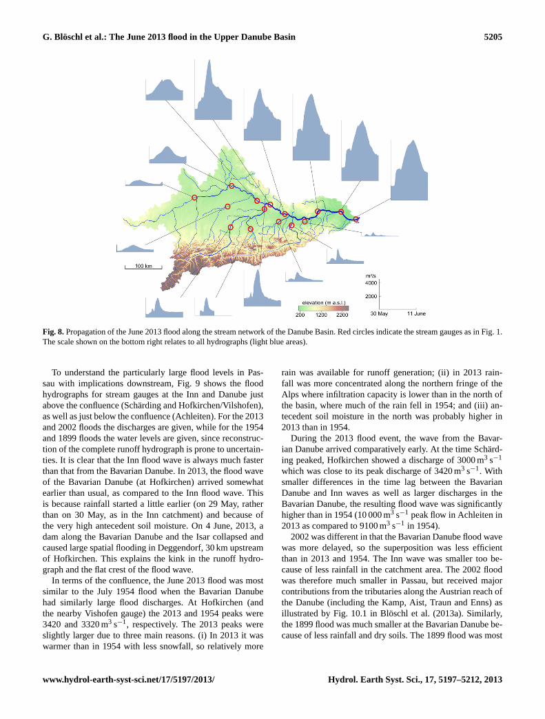
G. Blöschl et al.: The June 2013 flood in the Upper Danube Basin 5205
Fig. 8.Propagation of the June 2013 flood along the stream network of the Danube Basin. Red circles indicate the stream gauges as in Fig. 1.The scale shown on the bottom right relates to all hydrographs (light blue areas).
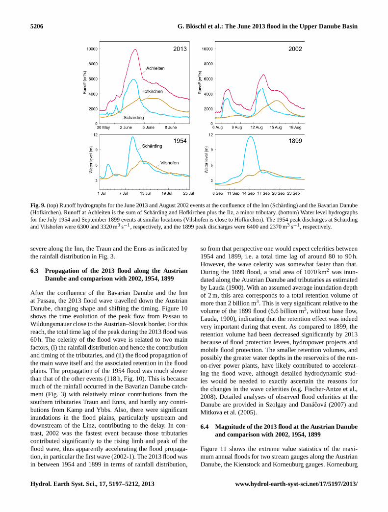
To understand the particularly large flood levels in Pas-sau with implications downstream, Fig. 9 shows the floodhydrographs for stream gauges at the Inn and Danube justabove the confluence (Schärding and Hofkirchen/Vilshofen),as well as just below the confluence (Achleiten). For the 2013and 2002 floods the discharges are given, while for the 1954and 1899 floods the water levels are given, since reconstruc-tion of the complete runoff hydrograph is prone to uncertain-ties. It is clear that the Inn flood wave is always much fasterthan that from the Bavarian Danube. In 2013, the flood waveof the Bavarian Danube (at Hofkirchen) arrived somewhatearlier than usual, as compared to the Inn flood wave. Thisis because rainfall started a little earlier (on 29 May, ratherthan on 30 May, as in the Inn catchment) and because ofthe very high antecedent soil moisture. On 4 June, 2013, adam along the Bavarian Danube and the Isar collapsed andcaused large spatial flooding in Deggendorf, 30 km upstreamof Hofkirchen. This explains the kink in the runoff hydro-graph and the flat crest of the flood wave.
In terms of the confluence, the June 2013 flood was mostsimilar to the July 1954 flood when the Bavarian Danubehad similarly large flood discharges. At Hofkirchen (andthe nearby Vishofen gauge) the 2013 and 1954 peaks were3420 and 3320 m3 s−1, respectively. The 2013 peaks wereslightly larger due to three main reasons. (i) In 2013 it waswarmer than in 1954 with less snowfall, so relatively more
rain was available for runoff generation; (ii) in 2013 rain-fall was more concentrated along the northern fringe of theAlps where infiltration capacity is lower than in the north ofthe basin, where much of the rain fell in 1954; and (iii) an-tecedent soil moisture in the north was probably higher in2013 than in 1954.
During the 2013 flood event, the wave from the Bavar-ian Danube arrived comparatively early. At the time Schärd-ing peaked, Hofkirchen showed a discharge of 3000 m3 s−1
which was close to its peak discharge of 3420 m3 s−1. Withsmaller differences in the time lag between the BavarianDanube and Inn waves as well as larger discharges in theBavarian Danube, the resulting flood wave was significantlyhigher than in 1954 (10 000 m3 s−1 peak flow in Achleiten in2013 as compared to 9100 m3 s−1 in 1954).
2002 was different in that the Bavarian Danube flood wavewas more delayed, so the superposition was less efficientthan in 2013 and 1954. The Inn wave was smaller too be-cause of less rainfall in the catchment area. The 2002 floodwas therefore much smaller in Passau, but received majorcontributions from the tributaries along the Austrian reach ofthe Danube (including the Kamp, Aist, Traun and Enns) asillustrated by Fig. 10.1 in Blöschl et al. (2013a). Similarly,the 1899 flood was much smaller at the Bavarian Danube be-cause of less rainfall and dry soils. The 1899 flood was most
5206 G. Blöschl et al.: The June 2013 flood in the Upper Danube Basin
Fig. 9. (top) Runoff hydrographs for the June 2013 and August 2002 events at the confluence of the Inn (Schärding) and the Bavarian Danube(Hofkirchen). Runoff at Achleiten is the sum of Schärding and Hofkirchen plus the Ilz, a minor tributary. (bottom) Water level hydrographsfor the July 1954 and September 1899 events at similar locations (Vilshofen is close to Hofkirchen). The 1954 peak discharges at Schärdingand Vilshofen were 6300 and 3320 m3 s−1, respectively, and the 1899 peak discharges were 6400 and 2370 m3 s−1, respectively.
severe along the Inn, the Traun and the Enns as indicated bythe rainfall distribution in Fig. 3.
6.3 Propagation of the 2013 flood along the AustrianDanube and comparison with 2002, 1954, 1899
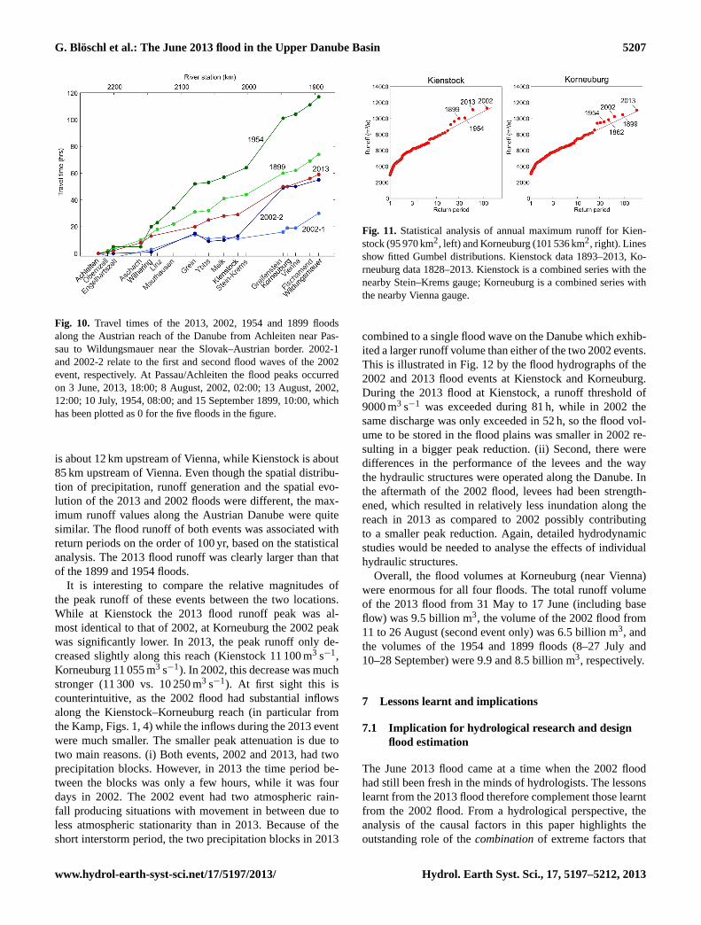
After the confluence of the Bavarian Danube and the Innat Passau, the 2013 flood wave travelled down the AustrianDanube, changing shape and shifting the timing. Figure 10shows the time evolution of the peak flow from Passau toWildungsmauer close to the Austrian–Slovak border. For thisreach, the total time lag of the peak during the 2013 flood was60 h. The celerity of the flood wave is related to two mainfactors, (i) the rainfall distribution and hence the contributionand timing of the tributaries, and (ii) the flood propagation ofthe main wave itself and the associated retention in the floodplains. The propagation of the 1954 flood was much slowerthan that of the other events (118 h, Fig. 10). This is becausemuch of the rainfall occurred in the Bavarian Danube catch-ment (Fig. 3) with relatively minor contributions from thesouthern tributaries Traun and Enns, and hardly any contri-butions from Kamp and Ybbs. Also, there were significantinundations in the flood plains, particularly upstream anddownstream of the Linz, contributing to the delay. In con-trast, 2002 was the fastest event because those tributariescontributed significantly to the rising limb and peak of theflood wave, thus apparently accelerating the flood propaga-tion, in particular the first wave (2002-1). The 2013 flood wasin between 1954 and 1899 in terms of rainfall distribution,
so from that perspective one would expect celerities between1954 and 1899, i.e. a total time lag of around 80 to 90 h.However, the wave celerity was somewhat faster than that.During the 1899 flood, a total area of 1070 km2 was inun-dated along the Austrian Danube and tributaries as estimatedby Lauda (1900). With an assumed average inundation depthof 2 m, this area corresponds to a total retention volume ofmore than 2 billion m3. This is very significant relative to thevolume of the 1899 flood (6.6 billion m3, without base flow,Lauda, 1900), indicating that the retention effect was indeedvery important during that event. As compared to 1899, theretention volume had been decreased significantly by 2013because of flood protection levees, hydropower projects andmobile flood protection. The smaller retention volumes, andpossibly the greater water depths in the reservoirs of the run-on-river power plants, have likely contributed to accelerat-ing the flood wave, although detailed hydrodynamic stud-ies would be needed to exactly ascertain the reasons forthe changes in the wave celerities (e.g. Fischer-Antze et al.,2008). Detailed analyses of observed flood celerities at theDanube are provided in Szolgay and Danácová (2007) andMitkova et al. (2005).
6.4 Magnitude of the 2013 flood at the Austrian Danubeand comparison with 2002, 1954, 1899
Figure 11 shows the extreme value statistics of the maxi-mum annual floods for two stream gauges along the AustrianDanube, the Kienstock and Korneuburg gauges. Korneuburg
G. Blöschl et al.: The June 2013 flood in the Upper Danube Basin 5207
Fig. 10. Travel times of the 2013, 2002, 1954 and 1899 floodsalong the Austrian reach of the Danube from Achleiten near Pas-sau to Wildungsmauer near the Slovak–Austrian border. 2002-1and 2002-2 relate to the first and second flood waves of the 2002event, respectively. At Passau/Achleiten the flood peaks occurredon 3 June, 2013, 18:00; 8 August, 2002, 02:00; 13 August, 2002,12:00; 10 July, 1954, 08:00; and 15 September 1899, 10:00, whichhas been plotted as 0 for the five floods in the figure.
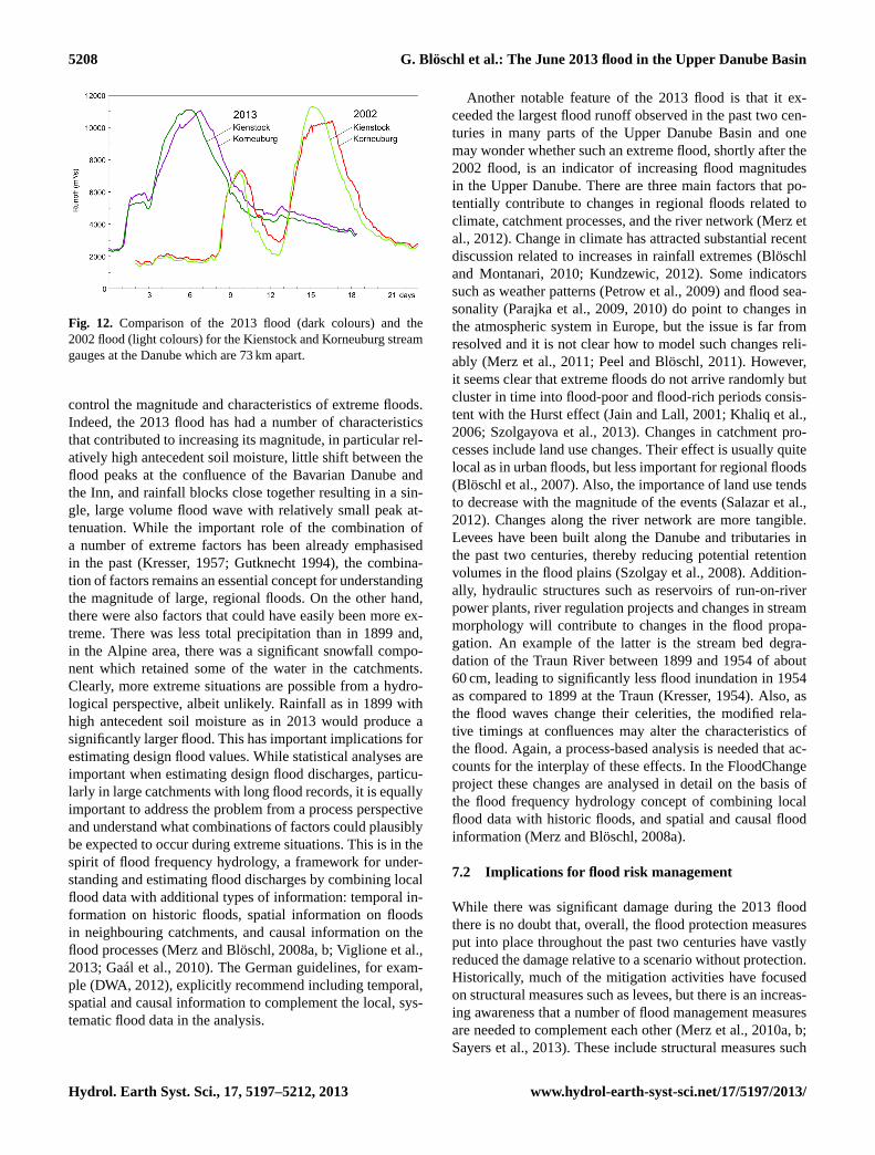
is about 12 km upstream of Vienna, while Kienstock is about85 km upstream of Vienna. Even though the spatial distribu-tion of precipitation, runoff generation and the spatial evo-lution of the 2013 and 2002 floods were different, the max-imum runoff values along the Austrian Danube were quitesimilar. The flood runoff of both events was associated withreturn periods on the order of 100 yr, based on the statisticalanalysis. The 2013 flood runoff was clearly larger than thatof the 1899 and 1954 floods.
It is interesting to compare the relative magnitudes ofthe peak runoff of these events between the two locations.While at Kienstock the 2013 flood runoff peak was al-most identical to that of 2002, at Korneuburg the 2002 peakwas significantly lower. In 2013, the peak runoff only de-creased slightly along this reach (Kienstock 11 100 m3 s−1,Korneuburg 11 055 m3 s−1). In 2002, this decrease was muchstronger (11 300 vs. 10 250 m3 s−1). At first sight this iscounterintuitive, as the 2002 flood had substantial inflowsalong the Kienstock–Korneuburg reach (in particular fromthe Kamp, Figs. 1, 4) while the inflows during the 2013 eventwere much smaller. The smaller peak attenuation is due totwo main reasons. (i) Both events, 2002 and 2013, had twoprecipitation blocks. However, in 2013 the time period be-tween the blocks was only a few hours, while it was fourdays in 2002. The 2002 event had two atmospheric rain-fall producing situations with movement in between due toless atmospheric stationarity than in 2013. Because of theshort interstorm period, the two precipitation blocks in 2013
Fig. 11. Statistical analysis of annual maximum runoff for Kien-stock (95 970 km2, left) and Korneuburg (101 536 km2, right). Linesshow fitted Gumbel distributions. Kienstock data 1893–2013, Ko-rneuburg data 1828–2013. Kienstock is a combined series with thenearby Stein–Krems gauge; Korneuburg is a combined series withthe nearby Vienna gauge.
combined to a single flood wave on the Danube which exhib-ited a larger runoff volume than either of the two 2002 events.This is illustrated in Fig. 12 by the flood hydrographs of the2002 and 2013 flood events at Kienstock and Korneuburg.During the 2013 flood at Kienstock, a runoff threshold of9000 m3 s−1 was exceeded during 81 h, while in 2002 thesame discharge was only exceeded in 52 h, so the flood vol-ume to be stored in the flood plains was smaller in 2002 re-sulting in a bigger peak reduction. (ii) Second, there weredifferences in the performance of the levees and the waythe hydraulic structures were operated along the Danube. Inthe aftermath of the 2002 flood, levees had been strength-ened, which resulted in relatively less inundation along thereach in 2013 as compared to 2002 possibly contributingto a smaller peak reduction. Again, detailed hydrodynamicstudies would be needed to analyse the effects of individualhydraulic structures.
Overall, the flood volumes at Korneuburg (near Vienna)were enormous for all four floods. The total runoff volumeof the 2013 flood from 31 May to 17 June (including baseflow) was 9.5 billion m3, the volume of the 2002 flood from11 to 26 August (second event only) was 6.5 billion m3, andthe volumes of the 1954 and 1899 floods (8–27 July and10–28 September) were 9.9 and 8.5 billion m3, respectively.
7 Lessons learnt and implications
7.1 Implication for hydrological research and designflood estimation
The June 2013 flood came at a time when the 2002 floodhad still been fresh in the minds of hydrologists. The lessonslearnt from the 2013 flood therefore complement those learntfrom the 2002 flood. From a hydrological perspective, theanalysis of the causal factors in this paper highlights theoutstanding role of thecombinationof extreme factors that
5208 G. Blöschl et al.: The June 2013 flood in the Upper Danube Basin
Fig. 12. Comparison of the 2013 flood (dark colours) and the2002 flood (light colours) for the Kienstock and Korneuburg streamgauges at the Danube which are 73 km apart.
control the magnitude and characteristics of extreme floods.Indeed, the 2013 flood has had a number of characteristicsthat contributed to increasing its magnitude, in particular rel-atively high antecedent soil moisture, little shift between theflood peaks at the confluence of the Bavarian Danube andthe Inn, and rainfall blocks close together resulting in a sin-gle, large volume flood wave with relatively small peak at-tenuation. While the important role of the combination ofa number of extreme factors has been already emphasisedin the past (Kresser, 1957; Gutknecht 1994), the combina-tion of factors remains an essential concept for understandingthe magnitude of large, regional floods. On the other hand,there were also factors that could have easily been more ex-treme. There was less total precipitation than in 1899 and,in the Alpine area, there was a significant snowfall compo-nent which retained some of the water in the catchments.Clearly, more extreme situations are possible from a hydro-logical perspective, albeit unlikely. Rainfall as in 1899 withhigh antecedent soil moisture as in 2013 would produce asignificantly larger flood. This has important implications forestimating design flood values. While statistical analyses areimportant when estimating design flood discharges, particu-larly in large catchments with long flood records, it is equallyimportant to address the problem from a process perspectiveand understand what combinations of factors could plausiblybe expected to occur during extreme situations. This is in thespirit of flood frequency hydrology, a framework for under-standing and estimating flood discharges by combining localflood data with additional types of information: temporal in-formation on historic floods, spatial information on floodsin neighbouring catchments, and causal information on theflood processes (Merz and Blöschl, 2008a, b; Viglione et al.,2013; Gaál et al., 2010). The German guidelines, for exam-ple (DWA, 2012), explicitly recommend including temporal,spatial and causal information to complement the local, sys-tematic flood data in the analysis.
Another notable feature of the 2013 flood is that it ex-ceeded the largest flood runoff observed in the past two cen-turies in many parts of the Upper Danube Basin and onemay wonder whether such an extreme flood, shortly after the2002 flood, is an indicator of increasing flood magnitudesin the Upper Danube. There are three main factors that po-tentially contribute to changes in regional floods related toclimate, catchment processes, and the river network (Merz etal., 2012). Change in climate has attracted substantial recentdiscussion related to increases in rainfall extremes (Blöschland Montanari, 2010; Kundzewic, 2012). Some indicatorssuch as weather patterns (Petrow et al., 2009) and flood sea-sonality (Parajka et al., 2009, 2010) do point to changes inthe atmospheric system in Europe, but the issue is far fromresolved and it is not clear how to model such changes reli-ably (Merz et al., 2011; Peel and Blöschl, 2011). However,it seems clear that extreme floods do not arrive randomly butcluster in time into flood-poor and flood-rich periods consis-tent with the Hurst effect (Jain and Lall, 2001; Khaliq et al.,2006; Szolgayova et al., 2013). Changes in catchment pro-cesses include land use changes. Their effect is usually quitelocal as in urban floods, but less important for regional floods(Blöschl et al., 2007). Also, the importance of land use tendsto decrease with the magnitude of the events (Salazar et al.,2012). Changes along the river network are more tangible.Levees have been built along the Danube and tributaries inthe past two centuries, thereby reducing potential retentionvolumes in the flood plains (Szolgay et al., 2008). Addition-ally, hydraulic structures such as reservoirs of run-on-riverpower plants, river regulation projects and changes in streammorphology will contribute to changes in the flood propa-gation. An example of the latter is the stream bed degra-dation of the Traun River between 1899 and 1954 of about60 cm, leading to significantly less flood inundation in 1954as compared to 1899 at the Traun (Kresser, 1954). Also, asthe flood waves change their celerities, the modified rela-tive timings at confluences may alter the characteristics ofthe flood. Again, a process-based analysis is needed that ac-counts for the interplay of these effects. In the FloodChangeproject these changes are analysed in detail on the basis ofthe flood frequency hydrology concept of combining localflood data with historic floods, and spatial and causal floodinformation (Merz and Blöschl, 2008a).
7.2 Implications for flood risk management
While there was significant damage during the 2013 floodthere is no doubt that, overall, the flood protection measuresput into place throughout the past two centuries have vastlyreduced the damage relative to a scenario without protection.Historically, much of the mitigation activities have focusedon structural measures such as levees, but there is an increas-ing awareness that a number of flood management measuresare needed to complement each other (Merz et al., 2010a, b;Sayers et al., 2013). These include structural measures such
G. Blöschl et al.: The June 2013 flood in the Upper Danube Basin 5209
as levees for flood protection and construction of polders forflood retention, and non-structural measures such as spatialplanning and increasing the preparedness of local citizens.Retaining water in polders and retention basins is always use-ful as, even for extreme flooding, flood attenuation will occurwith positive effects downstream. The drawback is that a lotof area is needed for flood retention to be effective for largerivers such as the Danube, as the flood peak reduction is adirect function of the available storage volume relative to theflood volume. In highly populated areas it is difficult to makesufficiently large areas available, so levees will continue toplay a central role in flood management. However, leveesmay exacerbate flood risk downstream. Integrated flood riskmanagement therefore considers the river basin as a whole asstipulated by the EU flood risk directive (EU, 2007).
Local protection of buildings, along with raising flood riskawareness and preparedness of local citizens, may be highlyeffective to complement the other measures. For these, andother flood event management measures such as early evac-uation and reliable warning systems driven by hydrologicalforecast models are needed. The maximum water level of the2013 flood was in fact predicted very well along the Aus-trian Danube for lead times between 24 and 48 h (depend-ing on the location), although the wave celerity was over-estimated (Blöschl et al., 2013c). While large-scale meteo-rological models and satellites provide important inputs, inparticular on future precipitation, capturing the local hydro-logical situation is essential for accurately modelling floods(Blöschl, 2008). Increasingly longer lead times are expectedfrom warning agencies, which requires the estimation offorecast uncertainties to quantify the confidence one has inthe predictions (Cloke and Pappenberger, 2009; Laurent etal., 2010; Komma et al., 2008; Nester et al., 2012). How-ever, communicating these uncertainties remains a challenge.Visualisation tools are one potential avenue towards assist-ing the communication (Ribicic et al., 2013; Hlavcová et al.,2005).
These flood management activities are important for allfloods that exceed bank full discharge and potentially pro-duce damage. Extreme floods, exceeding the June 2013 floodin magnitude, however, require special attention. A flood pro-duced by the 1899 rainfall with 2013 antecedent soil mois-ture is within the realm of thinkable situations, although itsprobability will be small. Some of the flood management ac-tivities will no longer be effective for a flood of that magni-tude. Instead, there is a need for an increased focus on reduc-ing the vulnerability of the system (Prudhomme et al., 2010;van Pelt and Swart, 2011; Blöschl et al., 2013b). Such mea-sures may not be optimum in an economic sense but may bemore robust than alternative approaches if a flood goes be-yond the limits of past experience. For example, the vulner-ability can be reduced by designing spillways for levees andby allowing for redundancy in warning systems and emer-gency plans. It is not unusual for the power system to failduring extreme floods, so redundancy is indeed important.
Land use planning and resettling activities to reduce the valueof assets in flood prone area will also contribute to reduc-ing the vulnerability. Participative processes are needed forsuch activities to find acceptability in a socio-economic con-text (Carr et al., 2012). From a long-term perspective, the in-terplay of socio-economic processes with hydrological pro-cesses is complex (Sivapalan et al., 2012; Di Baldassarre etal., 2013). In reducing vulnerability one may therefore startwith the policy options at the local scale and explore a widerange of possibilities causing extreme floods, including com-binations of unfavourable factors, and options for manag-ing them. The flood risk management study of Wardekker etal. (2010) is an example that explores imaginable surprises,something they term “wildcards”, to develop a strategy ofstrengthening the resilience of the city of Rotterdam. A re-silience approach may make the system less prone to dis-turbances and enable quick responses to make it capable ofdealing with extremes. For such extremes, as with all floods,the hallmark of integrated flood risk management is the in-terplay of all measures in a seamless way. Comparative floodanalysis studies as presented in this paper are an essentialbasis for developing more efficient strategies for integratedflood risk management.
Appendix A
Catchment characteristics
Table A1. Catchment area and mean elevation of the catchmentsused in this paper (Fig. 1).
Catchment Mean elevationStream gauge Stream area (km2) (m a.s.l.)
5210 G. Blöschl et al.: The June 2013 flood in the Upper Danube Basin
Acknowledgements.We would like to thank all the institutions thatprovided data, particularly the Hydrologic Offices and the CentralInstitute for Meteorology and Geodynamics. All data of the 2013flood are tentative. We would also like to thank the ERC (AdvancedGrant on FloodChange) and the FWF (project no P 23723-N21) forfinancial support.
Edited by: F. Pappenberger
References
BfG: Das Juni-Hochwasser des Jahres 2013 in Deutschland (The2013 June flood in Germany), BfG Report no. 1793, Federal In-stitute of Hydrology, Koblenz, Germany, 2013.
Blöschl, G.: Flood warning – on the value of local information, Int.J. River Basin Manage., 6, 41–50, 2008.
Blöschl, G. and Montanari, A.: Climate change impacts-throwingthe dice?, Hydrol. Process., 24, 374–381, 2010.
Blöschl, G., Ardoin-Bardin, S., Bonell, M., Dorninger, M.,Goodrich, D., Gutknecht, D., Matamoros, D., Merz, B., Shand,P., and Szolgay, J.: At what scales do climate variability and landcover change impact on flooding and low flows?, Hydrol. Pro-cess., 21, 1241–1247, 2007.
Blöschl, G., Sivapalan, M., Wagener, T., Viglione, A., and Savenije,H. H. G. (Eds.): Runoff Prediction in Ungauged Basins – Syn-thesis across Processes, Places and Scales, Cambridge UniversityPress, Cambridge, UK, 465 pp., 2013a.
Blöschl, G., Viglione, A., and Montanari, A.: Emerging approachesto hydrological risk management in a changing world, in: Cli-mate Vulnerability: Understanding and Addressing Threats toEssential Resources, Elsevier Inc., Academic Press, 3–10, 2013b.
Blöschl, G., Nester, Th., Komma, J., Parajka, J., and Perdigão, R. A.P.: Das Juni-Hochwasser 2013 – Analyse und Konsequenzen fürdas Hochwasserrisikomanagement (The June 2013 flood – analy-sis and implications for flood risk management), ÖsterreichischeIngenieur- und Architekten-Zeitschrift, 158, 141–152 , 2013c.
BLU (Bayerisches Landesamt für Umwelt): August – Hochwasser2005 in Südbayern (August 2005 flood in Southern Bavaria),Endbericht vom 12 April 2006, Bayerisches Landesamt fürUmwelt, München, 49 pp., 2006.
BMU: Hydrologischer Atlas von Deutschland (Hydrological Atlasof Germany), Bundesministerium für Umwelt, Naturschutz undReaktorsicherheit, Koblenz, 2003.
Carr, G., Blöschl, G., and Loucks, D. P.: Evaluating participation inwater resource management: A review, Water Resour. Res., 48,W11401, doi:10.1029/2011WR011662, 2012.
Cloke, H. L. and Pappenberger, F.: Ensemble flood forecasting: Areview, J. Hydrol., 375, 613–626, 2009.
Deutsche Vereinigung für Wasserwirtschaft, Abwasser und Ab-fall (DWA): Merkblatt Ermittlung von Hochwasserwahrschein-lichkeiten (Guidelines for estimating flood probabilities), DWA-M. 552, Hennef, Germany, 2012.
Di Baldassarre, G., Viglione, A., Carr, G., Kuil, L., Salinas, J.L., and Blöschl, G.: Socio-hydrology: conceptualising human-flood interactions, Hydrol. Earth Syst. Sci., 17, 3295–3303,doi:10.5194/hess-17-3295-2013, 2013.
EU: The European Parliament and the Council of the EuropeanUnion. Directive 2007/60/EC of the European Parliament and theCouncil of 23 October 2007 on the assessment and managementof flood risks, Off. J. Eur. Union, L288/27–L288/34, 2007.
Fischer-Antze, T., Olsen, N. R. B., and Gutknecht, D.: Three-dimensional CFD modeling of morphological bed changesin the Danube River, Water Resour. Res., 44, W09422,doi:10.1029/2007WR006402, 2008.
Gaál, L., Szolgay, J., Kohnová, S., Hlavcová, K., and Viglione, A.:Inclusion of historical information in flood frequency analysisusing a Bayesian MCMC technique: a case study for the powerdam Orlík, Czech Republic, in: Contributions to Geophysics andGeodesy, ISSN 1335-2806, Vol. 40, 121–147, 2010.
Gaál, L., Szolgay, J., Kohnová, S., Parajka, J., Merz, R.,Viglione, A., and Blöschl, G.: Flood timescales: Understand-ing the interplay of climate and catchment processes throughcomparative hydrology, Water Resour. Res., 48, W04511,doi:10.1029/2011WR011509, 2012.
Godina, R., Lalk, P., Lorenz, P., Müller, G., and Weilguni, V.: DieHochwasserereignisse im Jahr 2002 in Österreich (The floodevents of 2002 in Austria), Mitt. Hydrogr. Dienstes Österreich,82, 1– 39, 2003.
Gutknecht, D.: Extremhochwässer in kleinen Einzugsgebieten (Ex-treme floods in small catchments), Österreichische Wasser- undAbfallwirtschaft, 46, 50–57, 1994.
Gutknecht, D., Reszler, Ch., und Blöschl, G.: Das Katastrophen-hochwasser vom 7. August 2002 am Kamp – eine erste Ein-schätzung (The 7 August 2002 – flood of the Kamp – a firstassessment), Elektrotechnik und Informationstechnik, 119, 411–413, 2002.
Haiden, T., Kann, A., Wittmann, C., Pistotnik, G., Bica, B., andGruber, C.: The integrated nowcasting through comprehensiveanalysis (INCA) system and its validation over the eastern Alpineregion, Weather Forecast., 26, 166–183, 2011.
Hlavcová, H., Kohnova, S., Kubeš, R., Szolgay, J., and Zv-olensky, M.: An empirical method for estimating future floodrisks for flood warnings, Hydrol. Earth Syst. Sci., 9, 431–448,doi:10.5194/hess-9-431-2005, 2005.
Holton, J. R.: An introduction to Dynamic Meteorology, Elsevier,4th Edition, 535 pp., 2004.
HZB: Das Juli-Hochwasser 1954 im österreichischen Donaugebiet(The July 1954 flood in the Austrian Danube basin), Beiträge zurHydrographie Österreichs, Nr. 29, Hydrogr. Zentralbüro Wien,139 pp., 1955.
Jain, S. and Lall, U.: Floods in a changing climate: Does the pastrepresent the future?, Water Resour. Res., 37, 3193–3205, 2001.
Janoschek, W. R. and Matura, A.: Outline of the Geology of Austria,Abb. Geol. B.-A., 26e, 7–98, 1980.
Khaliq, M. N., Ouarda, T. B. M. J., Ondo, J.-C., Gachon, P., andBobée, B.: Frequency analysis of a sequence of dependent and/ornon-stationary hydro-meteorological observations: A review, J.Hydrol., 329, 534–552, 2006.
Kistler, R., Kalnay, E., Collins, W., Saha, S., White, G., Woollen,J., Chelliah, M., Ebisuzaki, W., Kanamitsu, M., Kousky, V., vanden Dool, H., Jenne, R., and Fiorino, M.: The NCEP-NCAR 50-Year Reanalysis: Monthly Means CD-ROM and Documentation,B. Am. Meteorol. Soc., 82, 247–268, 2001.
Kresser, W.: Der Einfluß der Regulierungs- und Kraftwerksbautenauf die Hochwasserverhältnisse der österreichische Donau (Ef-fect of river training and power plants on the floods of theAustrian Danube), Oesterreichische Wasserwirtschaft 6, 65–68,1954.
Kresser, W.: Die Hochwässer der Donau (The floods ofthe Danube), Schriftenreihe des österreichischen Wasser-wirtschaftsverbandes, 32–33, Wien, 1957.
Kundzewicz, Z. W. (Ed.): Changes in Flood Risk in Europe, IAHSSpecial Publication 10, IAHS Press, Wallingford, 516 pp., 2012.
Lauda, E.: Die Hochwasserkatastrophe des Jahres 1899 im österre-ichischen Donaugebiete (The flood disaster of 1899 in the Aus-trian Danube basin), Beiträge zur Hydrographie Österreichs, IV.Heft, k.k. hydrographisches Central-Bureau, Wien, 1900.
Laurent, S., Hangen-Brodersen, C., Ehret, U., Meyer, I., Moritz, K.,Vogelbacher, A., and Holle, F.-K.: Forecast Uncertainties in theOperational Flood Forecasting of the Bavarian Danube Catch-ment, in: Hydrological Processes of the Danube River Basin,edited by: Brilly, M., Springer, 367–387, 2010.
Merz, B., Kreibich, H., Schwarze, R., and Thieken, A.: Reviewarticle “Assessment of economic flood damage”, Nat. HazardsEarth Syst. Sci., 10, 1697–1724, doi:10.5194/nhess-10-1697-2010, 2010a.
Merz, B., Hall, J., Disse, M., and Schumann, A.: Fluvial flood riskmanagement in a changing world, Nat. Hazards Earth Syst. Sci.,10, 509–527, doi:10.5194/nhess-10-509-2010, 2010b.
Merz, B., Vorogushyn, S., Uhlemann, S., Delgado, J., and Hun-decha, Y.: HESS Opinions “More efforts and scientific rigourare needed to attribute trends in flood time series”, Hydrol.Earth Syst. Sci., 16, 1379–1387, doi:10.5194/hess-16-1379-2012, 2012.
Merz, R. and Blöschl, G.: Flood frequency hydrology: 1. Temporal,spatial, and causal expansion of information, Water Resour. Res.,44, W08432, 2008a.
Merz, R. and Blöschl, G.: Flood frequency hydrology: 2. Combin-ing data evidence, Water Resour. Res., 44, W08433, 2008b.
Merz, R. and Blöschl, G.: A regional analysis of event runoffcoefficients with respect to climate and catchment char-acteristics in Austria, Water Resour. Res., 45, W01405,doi:10.1029/2008WR007163, 2009.
Merz, R., Blöschl, G., and Parajka, J.: Spatio-temporal variabilityof event runoff coefficients in Austria, J. Hydrol., 331, 591–604,2006.
Merz, R., Parajka, J., and Blöschl, G.: Time stability of catchmentmodel parameters: Implications for climate impact analyses,Water Resour. Res., 47, W02531, doi:10.1029/2010WR009505,2011.
Mitkova, V., Pekarova, P., Miklanek, P., and Pekar, J.: Analysis offlood propagation changes in the Kienstock–Bratislava reach ofthe Danube River, Hydrolog. Sci. J., 50, 655–668, 2005.
Nester, T., Kirnbauer, R., Gutknecht, D., and Blöschl, G.: Climateand catchment controls on the performance of regional flood sim-ulations, J. Hydrol., 402, 340–356, 2011.
Nester, T., Komma, J., Viglione, A., and Blöschl, G.: Flood forecasterrors and ensemble spread – a case study, Water Resour. Res.,48, W10502, doi:10.1029/2011WR011649, 2012.
Parajka, J., Merz, R., and Blöschl, G.: Uncertainty and multiple ob-jective calibration in regional water balance modeling – Casestudy in 320 Austrian catchments, Hydrol. Process., 21, 435–446, 2007.
Parajka, J., Kohnová, S., Merz, R., Szolgay, J., Hlavcová, K., andBlöschl, G.: Comparative analysis of the seasonality of hydro-logical characteristics in Slovakia and Austria, Hydrolog. Sci. J.,54, 456–473, 2009.
Parajka, J., Kohnová, S., Bálint, G., Barbuc, M., Borga, M., Claps,P., Cheval, S., Dumitrescu, A., Gaume, E., Hlavcová, K., Merz,R., Pfaundler, M., Stancalie, G., Szolgay, J., and Blöschl, G.:Seasonal characteristics of flood regimes across the Alpine–Carpathian range, J. Hydrol., 394, 78–89, 2010.
Peel, M. C. and Blöschl, G.: Hydrologic modelling in a changingworld, Prog. Phys. Geogr., 35, 249–261, 2011.
Pekarová, P., Halmová, D., Bacová-Mitková, V., Miklánek, P.,Pekár, J., and Škoda, P: Historic flood marks and flood frequencyanalysis of the Danube River at Bratislava, Slovakia, J. Hydrol.Hydromech., 61, 326–333, doi:10.2478/johh-2013-0041, 2013.
Petrow, T., Zimmer, J., and Merz, B.: Changes in the flood hazardin Germany through changing frequency and persistence of cir-culation patterns, Nat. Hazards Earth Syst. Sci., 9, 1409–1423,doi:10.5194/nhess-9-1409-2009, 2009.
Prudhomme, C., Wilby, R., Crooks, S., Kay, A., and Reynard, N.:Scenario-neutral approach to climate change impact studies: Ap-plication to flood risk, J. Hydrol., 390, 198–209, 2010.
Ribicic, H., Waser, J., Fuchs, R., Blöschl, G., and Gröller, E.: Vi-sual analysis and steering of flooding simulations. IEEE T. Vis.Comput. Gr., 19, 1062–1075, 2013.
Rossby, C.-G.: Relation between variations in the intensity of thezonal circulation of the atmosphere and the displacements of thesemi-permanent centers of action, J. Mar. Res., 2, 38–55, 1939.
Salazar, S., Francés, F., Komma, J., Blume, T., Francke, T., Bron-stert, A., and Blöschl, G.: A comparative analysis of the effec-tiveness of flood management measures based on the concept of“retaining water in the landscape” in different European hydro-climatic regions, Nat. Hazards Earth Syst. Sci., 12, 3287–3306,doi:10.5194/nhess-12-3287-2012, 2012.
Sayers, P. Y. L. I., Galloway, G., Penning-Rowsell, E., Shen, F.,Wen, K., Chen, Y., and Le Quesne, T.: Flood Risk Management:A Strategic Approach. Paris, UNESCO, 2013.
Schmidt, M. (Ed.): Hochwasser und Hochwasserschutz in Deutsch-land vor 1850 (Floods and flood protection in Germany before1850), Oldenbourd Industrieverlag, Munich, ISBN 3-486-26494-x, 280 pp., 2000.
Sivapalan, M., Savenije, H. H. G., and Blöschl, G.: Socio-hydrology: A new science of people and water, Hydrol. Process.,26, 1270–1276, 2012.
Szolgay, J. and Danácová, M.: Detection of changes in the floodcelerity by multilinear routing on the Danube, Meteorol. J., 10,219–224, 2007.
5212 G. Blöschl et al.: The June 2013 flood in the Upper Danube Basin
Szolgay, J., Danáèová, M., Jurèák, S., and Spál, P.: Multilinear floodrouting using empirical wave-speed discharge relationships: casestudy on the Morava River, J. Hydrol. Hydromech., 56, 213–227,2008.
Szolgayova, E., Laaha, G., Blöschl, G., and Bucher, C.: Fac-tors influencing long range dependence in streamflow of Euro-pean rivers, Hydrol. Process., online first, doi:10.1002/hyp.9694,2013.
Ulbrich, U., Brücher, T., Fink, A. H., Leckebusch, G. C., Krüger, A.,and Pinto, J. G.: The central European floods of August 2002:Part 1 – Rainfall periods and flood development, Weather, 58,371–377, 2003.
van Bebber, W. J.: Die Zugstrassen der barometrischen Min-ima nach den Bahnenkarten der Deutschen Seewarte für denZeitraum von 1870–1890, Meteorol. Z., 8, 361–366, 1891.
van Pelt, S. C. and Swart, R. J.: Climate change risk managementin transnational river basins: the Rhine, Water Resour. Manage.,25, 3837–3861, 2011.
Viglione, A., Chirico, G. B., Komma, J., Woods, R., Borga, M.,and Blöschl, G.: Quantifying space–time dynamics of flood eventtypes, J. Hydrol., 394, 213–229, 2010.
Viglione, A., Merz, R., Salinas, J. S., and Blöschl, G.: Flood fre-quency hydrology: 3. A Bayesian analysis, Water Resour. Res.,49, 675–692, 2013.
Wardekker, J. A., de Jong, A., Knoop, J. M., and van der Sluijs, J.P.: Operationalising a resilience approach to adapting an urbandelta to uncertain climate changes, Technol. Forecast. Soc., 77,987–998, 2010.