Morbidelli and Brown: Kuiper Belt and Evolution of Solar System 175

175

The Kuiper Belt and the PrimordialEvolution of the Solar System

A. MorbidelliObservatoire de la Côte d’Azur

M. E. BrownCalifornia Institute of Technology

We discuss the structure of the Kuiper belt as it can be inferred from the first decade ofobservations. In particular, we focus on its most intriguing properties — the mass deficit, theinclination distribution, and the apparent existence of an outer edge and a correlation amonginclinations, colors, and sizes — which clearly show that the belt has lost the pristine structureof a dynamically cold protoplanetary disk. Understanding how the Kuiper belt acquired itspresent structure will provide insight into the formation of the outer planetary system and itsearly evolution. We critically review the scenarios that have been proposed so far for the pri-mordial sculpting of the belt. None of them can explain in a single model all the observedproperties; the real history of the Kuiper belt probably requires a combination of some of theproposed mechanisms.

1. INTRODUCTION

When Edgeworth and Kuiper conjectured the existenceof a belt of small bodies beyond Neptune — now knownas the Kuiper belt — they certainly were imagining a diskof planetesimals that preserved the pristine conditions of theprotoplanetary disk. However, since the first discoveries oftransneptunian objects, astronomers have realized that thispicture is not correct: The disk has been affected by a num-ber of processes that have altered its original structure. TheKuiper belt may thus provide us with many clues to under-stand what happened in the outer solar system during theprimordial ages. Potentially, the Kuiper belt might teach usmore about the formation of the giant planets than the plan-ets themselves. And, as in a domino effect, a better knowl-edge of giant-planet formation would inevitably boost ourunderstanding of the subsequent formation of the terrestrialplanets. Consequently, Kuiper belt research is now consid-ered a top priority in modern planetary science.

A decade after the discovery of 1992 QB1 (Jewitt andLuu, 1993), we now know 770 transneptunian objects (semi-major axis a > 30 AU) (all numbers are as of March 3,2003). Of these, 362 have been observed during at least twooppositions, and 239 during at least three oppositions. Ob-servations at two and three oppositions are necessary forthe Minor Planet Center to compute the objects’ orbital ele-ments with moderate and good accuracy respectively. There-fore, the transneptunian population is gradually taking shape,and we can start to seriously examine the Kuiper belt struc-ture and learn what it has to teach us. We should not forget,however, that our view of the transneptunian population isstill partial and is strongly biased by a number of factors,some of which cannot be easily modeled.

A primary goal of this chapter is to present the orbitalstructure of the Kuiper belt as it stands based on the currentobservations. We start in section 2 by presenting the varioussubclasses that constitute the transneptunian population.Then in section 3 we describe some striking properties ofthe population, such as its mass deficit, inclination excita-tion, radial extent and a puzzling correlation between or-bital elements and physical properties. In section 4 wefinally review the models that have been proposed so faron the primordial sculpting of the Kuiper belt. Some ofthese models date from the very beginning of Kuiper beltscience, when only a handful of objects were known, andhave been at least partially invalidated by the new data.Paradoxically, however, as the data increase in number andquality, it becomes increasingly difficult to explain all theproperties of the Kuiper belt in the framework of a singlescenario. The conclusions are in section 5.

2. TRANSNEPTUNIAN POPULATIONS

The transneptunian population is “traditionally” subdi-vided in two subpopulations: the scattered disk and the Kui-per belt. The definition of these subpopulations is not uni-form, as the Minor Planet Center and various authors oftenuse slightly different criteria. Here we propose and discussa categorization based on the dynamics of the objects andtheir relevance to the reconstruction of the primordial evo-lution of the outer solar system.

In principle, one would like to call the Kuiper belt thepopulation of objects that, even if characterized by chaoticdynamics, do not suffer close encounters with Neptune andthus do not undergo macroscopic migration in semimajoraxis. Conversely, the bodies that are transported in semi-

176 Comets II

major axis by close and distant encounters with Neptunewould constitute the scattered disk. The problem with pre-cisely dividing the transneptunian population into Kuiperbelt or scattered disk is related to timescale. On what time-scale should we see semimajor axis migration resulting inthe classification of an object in the scattered disk? Thequestion is relevant, because it is possible for bodies trappedin resonances to significantly change their perihelion dis-tance and pass from a scattering phase to a nonscatteringphase (and vice versa) numerous times over the age of thesolar system.

For this reason, we prefer to link the definition of thescattered disk to its formation mechanism. We refer to thescattered disk as the region of orbital space that can bevisited by bodies that have encountered Neptune within aHill’s radius at least once during the age of the solar sys-tem, assuming no substantial modification of the planetaryorbits. We then refer to the Kuiper belt as the complementof the scattered disk in the a > 30 AU region.

To categorize the observed transneptunian bodies intoscattered disk and Kuiper belt, we refer to previous workon the dynamics of transneptunian bodies in the frameworkof the current architecture of the planetary system. For thea < 50 AU region, we use the results by Duncan et al. (1995)and Kuchner et al. (2002), who numerically mapped the re-

gions of the (a, e, i) space with 32 < a < 50 AU that canlead to a Neptune-encountering orbit within 4 G.y. Becausedynamics are reversible, these are also the regions that canbe visited by a body after having encountered the planet.Therefore, according to our definition, they constitute thescattered disk. For the a > 50 AU region, we use the resultsby Levison and Duncan (1997) and Duncan and Levison(1997), who followed for a time span of another 4 G.y. theevolutions of the particles that encountered Neptune inDuncan et al. (1995). Despite the fact that the initial condi-tions did not cover all possible configurations, we can rea-sonably assume that these integrations cumulatively showthe regions of the orbital space that can be possibly visitedby bodies transported to a > 50 AU by Neptune encounters.Again, according to our definition, these regions constitutethe scattered disk.

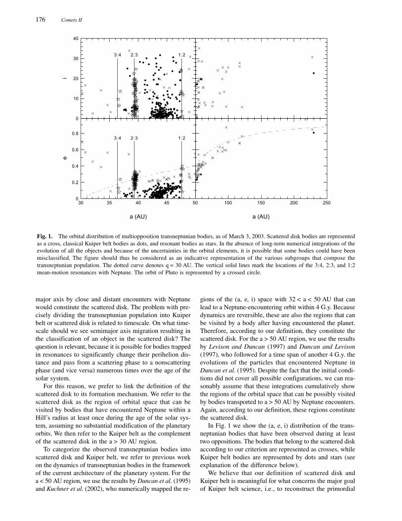
In Fig. 1 we show the (a, e, i) distribution of the trans-neptunian bodies that have been observed during at leasttwo oppositions. The bodies that belong to the scattered diskaccording to our criterion are represented as crosses, whileKuiper belt bodies are represented by dots and stars (seeexplanation of the difference below).

We believe that our definition of scattered disk andKuiper belt is meaningful for what concerns the major goalof Kuiper belt science, i.e., to reconstruct the primordial

Fig. 1. The orbital distribution of multiopposition transneptunian bodies, as of March 3, 2003. Scattered disk bodies are representedas a cross, classical Kuiper belt bodies as dots, and resonant bodies as stars. In the absence of long-term numerical integrations of theevolution of all the objects and because of the uncertainties in the orbital elements, it is possible that some bodies could have beenmisclassified. The figure should thus be considered as an indicative representation of the various subgroups that compose thetransneptunian population. The dotted curve denotes q = 30 AU. The vertical solid lines mark the locations of the 3:4, 2:3, and 1:2mean-motion resonances with Neptune. The orbit of Pluto is represented by a crossed circle.

Morbidelli and Brown: Kuiper Belt and Evolution of Solar System 177

evolution of the outer solar system. In fact, all bodies inthe solar system must have been formed on orbits with verysmall eccentricities and inclinations, typical of an accretiondisk. In the framework of the current architecture of thesolar system, the current orbits of scattered disk bodiesmight have started with quasicircular orbits in Neptune’szone by pure dynamical evolution. Therefore, they do notprovide any relevant clue to uncover the primordial archi-tecture. The opposite is true for the orbits of the Kuiper beltobjects with nonnegligible eccentricity and/or inclination.Their existence reveals that some excitation mechanism thatis no longer at work occurred in the past (see section 4).

In this respect, the existence of Kuiper belt bodies witha > 50 AU on highly eccentric orbits is particularly impor-tant (five objects in Fig. 1, although our classification is un-certain for the reasons explained in the figure caption).Among them, 2000 CR105 (a = 230 AU, perihelion distanceq = 44.17 AU, and inclination i = 22.7°) is a challenge byitself concerning the explanation of its origin. We call theseobjects extended scattered disk objects for two reasons:(1) they do not belong to the scattered disk according toour definition but are very close to its boundary and (2) abody of ~300 km like 2000 CR105 presumably formed muchcloser to the Sun, where the accretion timescale was suffi-ciently short (Stern, 1996), implying that it has been sub-sequently transported in semimajor axis until reaching itscurrent location. This hypothesis suggests that in the pastthe true scattered disk extended well beyond its presentboundary in perihelion distance. Given that the observa-tional biases rapidly become more severe with increasingperihelion distance and semimajor axis, the currently knownextended scattered disk objects may be the tip of the ice-berg, e.g., the emerging representatives of a conspicuouspopulation, possibly outnumbering the scattered disk popu-lation (Gladman et al., 2002).

In addition to the extended scattered disk, we distinguishtwo other subpopulations of the Kuiper belt. We refer tothe Kuiper belt bodies that are located in some major mean-motion resonance with Neptune [essentially the 3:4, 2:3,and 1:2 resonances (star symbols in Fig. 1) but also the 2:5resonance (see Chiang et al., 2003)] as the resonant popu-lation. It is well known that mean-motion resonances offera protection mechanism against close encounters with theresonant planet (Cohen and Hubbard, 1965). For this rea-son, the resonant population — which, as part of the Kuiperbelt, by definition must not encounter Neptune within theage of the solar system — can have perihelion distancesmuch smaller than the other Kuiper belt objects, and evenNeptune-crossing orbits (q < 30 AU) as in the case of Pluto.The bodies in the 2:3 resonance are often called Plutinosbecause of the analogy of their orbit with that of Pluto. Wecall the collection of Kuiper belt objects with a < 50 AUthat are not in any notable resonant configuration the clas-sical belt. Because they are not protected from close en-counters with Neptune by any resonance, the stability cri-terion confines them to the region with small to moderateeccentricity, typically on orbits with q > 35 AU. The adjec-tive “classical” is justified because, among all subpopula-

tions, this is the one whose orbital properties are the mostsimilar to those expected for the Kuiper belt prior to thefirst discoveries. We note, however, that the classical popu-lation is not that “classical.” Although moderate, the eccen-tricities are larger than those that should characterize a proto-planetary disk. Moreover, several bodies have very largeinclinations (see section 3.2). Finally, the total mass is onlya small fraction of the expected pristine mass in that region(section 3.1). All these elements indicate that the classicalbelt has also been affected by some primordial excitationand depletion mechanism(s).

3. STRUCTURE OF THE KUIPER BELT

3.1. Missing Mass of the Kuiper Belt

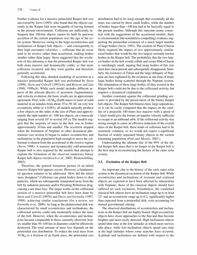
The original argument followed by Kuiper (1951) to con-jecture the existence of a band of small planetesimals be-yond Neptune was related to the mass distribution in theouter solar system. The minimum mass solar nebula inferredfrom the total planetary mass (plus lost volatiles) smoothlydeclines from the orbit of Jupiter until the orbit of Neptune(see Fig. 2); why should it abruptly drop beyond the lastplanet? However, while Kuiper’s conjecture on the exist-ence of a transneptunian belt is correct, the total mass inthe 30–50-AU range inferred from observations is two or-ders of magnitude smaller than the one he expected.

Kuiper’s argument is not the only indication that the massof the primordial Kuiper belt had to be significantly larger.

Fig. 2. The mass distribution of the solar nebula inferred fromthe masses of the planets augmented by the mass needed to bringthe observed material to solar composition (data from Lewis,1995). The surface density in the Kuiper belt has been computedassuming a current mass of ~0.1 M (Jewitt et al., 1996; Chiangand Brown, 1999; Trujillo et al., 2001; Gladman et al., 2001) inthe 42–48-AU annulus, and scaling the result by a factor of 70 inorder to account for the inferred primordial local ratio betweenvolatiles and solids. The estimate of the total mass in the Kuiperbelt overwhelms that of Pluto, but still does not bring the mass tothe extrapolation of the ~r–3/2 line.

178 Comets II

Further evidence for a massive primordial Kuiper belt wasuncovered by Stern (1995), who found that the objects cur-rently in the Kuiper belt were incapable of having formedin the present environment: Collisions are sufficiently in-frequent that 100-km objects cannot be built by pairwiseaccretion of the current population over the age of the so-lar system. Moreover, owing to the large eccentricities andinclinations of Kuiper belt objects — and consequently totheir high encounter velocities — collisions that do occurtend to be erosive rather than accretional, making bodiessmaller rather than larger. Stern suggested that the resolu-tion of this dilemma is that the primordial Kuiper belt wasboth more massive and dynamically colder, so that morecollisions occurred, and they were gentler and thereforegenerally accretional.

Following this idea, detailed modeling of accretion in amassive primordial Kuiper belt was performed by Stern(1996), Stern and Colwell (1997a,b), and Kenyon and Luu(1998, 1999a,b). While each model includes different as-pects of the relevant physics of accretion, fragmentation,and velocity evolution, the basic results are in approximateagreement. First, with ~10 M (Earth mass) or more of solidmaterial in an annulus from about 35 to 50 AU on very loweccentricity orbits (e ≤ 0.001), all models naturally producea few objects on the order of the size of Pluto and approxi-mately the right number of ~100-km objects, on a timescaleranging from several 107 to several 108 yr. The models sug-gest that the majority of mass in the disk was in bodiesapproximately 10 km and smaller. The accretion stoppedwhen the formation of Neptune or other dynamical phe-nomena (see section 4) began to induce eccentricities andinclinations in the population high enough to move the col-lisional evolution from the accretional to the erosive regime(Stern, 1996). A massive and dynamically cold primordialKuiper belt is also required by the models that attempt toexplain the formation of the observed numerous binaryKuiper belt objects (Goldreich et al., 2002; Weidenshilling,2002).

Therefore, the general formation picture of an initialmassive Kuiper belt appears secure. However, a fundamen-tal question remains to be addressed: How did the initialmass disappear? Collisions can grind bodies down to dustparticles, which are subsequently transported away from thebelt by radiation pressure and/or Poynting Robertson drag,causing a net mass loss. The major works on the collisionalerosion of a massive primordial belt have been done byStern and Colwell (1997b) and Davis and Farinella (1997,1998), achieving similar conclusions (for a review, seeFarinella et al., 2000). As long as the planetesimal disk wascharacterized by small eccentricities and inclinations, thecollisional activity could only moderately reduce the massof the belt. However, when the eccentricities and inclina-tions became comparable to those currently observed, bod-ies smaller than 50–100 km in diameter could be effectivelydestroyed. The total amount of mass loss depends on theprimordial size distribution. To reduce the total mass from30 M to a fraction of an Earth mass, the primordial size

distribution had to be steep enough that essentially all themass was carried by these small bodies, while the numberof bodies larger than ~100 km had to be basically equal tothe present number. Although this outcome seems consis-tent with the suggestions of the accretional models, thereis circumstantial (but nonetheless compelling) evidence sug-gesting the primordial existence of a much larger numberof large bodies (Stern, 1991). The creation of Pluto-Charonlikely required the impact of two approximately similar-sized bodies that would be the two largest currently knownbodies in the Kuiper belt. The probability that the two larg-est bodies in the belt would collide and create Pluto-Charonis vanishingly small, arguing that many bodies of this sizemust have been present and subsequently disappeared. Simi-larly, the existence of Triton and the large obliquity of Nep-tune are best explained by the existence at one time of manylarge bodies being scattered through the Neptune system.The elimination of these large bodies (if they existed in theKuiper belt) could not be due to the collisional activity, butrequires a dynamical explanation.

Another constraint against the collisional grinding sce-nario is provided by the preservation of the binary Kuiperbelt objects. The Kuiper belt binaries have large separations,so it can be easily computed that the impact on the satel-lite of a projectile 100 times less massive with a speed of1 km/s would give the former an impulse velocity sufficientto escape to an unbound orbit. If the collisional activity wasstrong enough to cause an effective reduction of the overallmass of the Kuiper belt, these kinds of collisions had to beextremely common, so we would not expect a significantfraction of widely separated binary objects in the currentremaining population (Petit and Mousis, 2003.)

Understanding the ultimate fate of the 99% of the ini-tial Kuiper belt mass that is no longer in the Kuiper belt isthe first step in reconstructing the history of the outer solarsystem.

3.2. Excitation of the Kuiper Belt

An important clue to the history of the early outer solarsystem is the dynamical excitation of the Kuiper belt. Whileeccentricities and inclinations of resonant and scatteredobjects are expected to have been affected by interactionswith Neptune, those of the classical objects should havesuffered no such excitation. Nonetheless, the confirmedclassical belt objects have an inclination range up to at least32° and an eccentricity range up to 0.2, significantly higherthan expected from a primordial disk, even accounting formutual gravitational stirring.

The observed distributions of eccentricities and inclina-tions in the Kuiper belt are highly biased. High-eccentricityobjects have closer approaches to the Sun and thus becomebrighter and more easily detected. High-inclination objectsspend little time at the low latitudes at which most surveystake place, while low-inclination objects spend zero timeat the high latitudes where some searches have occurred.(Latitude and inclination are defined with respect to the

Morbidelli and Brown: Kuiper Belt and Evolution of Solar System 179

invariable plane, which is a better representation for theplane of the Kuiper belt than is the ecliptic.)

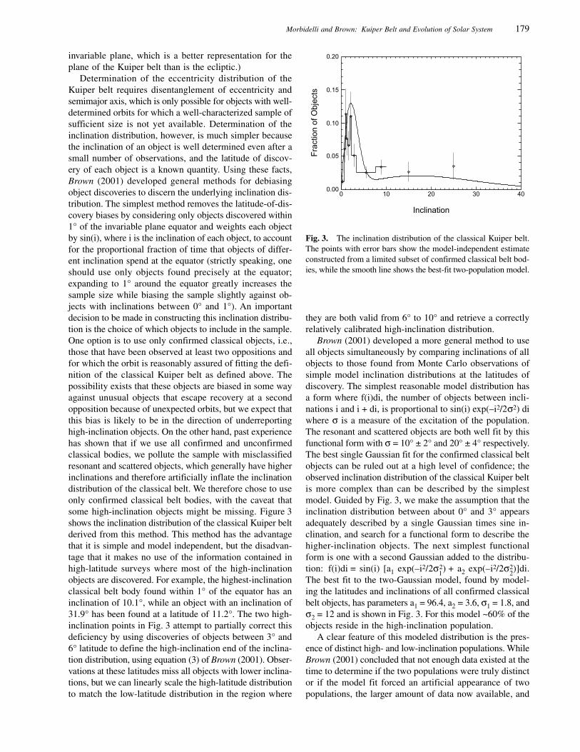
Determination of the eccentricity distribution of theKuiper belt requires disentanglement of eccentricity andsemimajor axis, which is only possible for objects with well-determined orbits for which a well-characterized sample ofsufficient size is not yet available. Determination of theinclination distribution, however, is much simpler becausethe inclination of an object is well determined even after asmall number of observations, and the latitude of discov-ery of each object is a known quantity. Using these facts,Brown (2001) developed general methods for debiasingobject discoveries to discern the underlying inclination dis-tribution. The simplest method removes the latitude-of-dis-covery biases by considering only objects discovered within1° of the invariable plane equator and weights each objectby sin(i), where i is the inclination of each object, to accountfor the proportional fraction of time that objects of differ-ent inclination spend at the equator (strictly speaking, oneshould use only objects found precisely at the equator;expanding to 1° around the equator greatly increases thesample size while biasing the sample slightly against ob-jects with inclinations between 0° and 1°). An importantdecision to be made in constructing this inclination distribu-tion is the choice of which objects to include in the sample.One option is to use only confirmed classical objects, i.e.,those that have been observed at least two oppositions andfor which the orbit is reasonably assured of fitting the defi-nition of the classical Kuiper belt as defined above. Thepossibility exists that these objects are biased in some wayagainst unusual objects that escape recovery at a secondopposition because of unexpected orbits, but we expect thatthis bias is likely to be in the direction of underreportinghigh-inclination objects. On the other hand, past experiencehas shown that if we use all confirmed and unconfirmedclassical bodies, we pollute the sample with misclassifiedresonant and scattered objects, which generally have higherinclinations and therefore artificially inflate the inclinationdistribution of the classical belt. We therefore chose to useonly confirmed classical belt bodies, with the caveat thatsome high-inclination objects might be missing. Figure 3shows the inclination distribution of the classical Kuiper beltderived from this method. This method has the advantagethat it is simple and model independent, but the disadvan-tage that it makes no use of the information contained inhigh-latitude surveys where most of the high-inclinationobjects are discovered. For example, the highest-inclinationclassical belt body found within 1° of the equator has aninclination of 10.1°, while an object with an inclination of31.9° has been found at a latitude of 11.2°. The two high-inclination points in Fig. 3 attempt to partially correct thisdeficiency by using discoveries of objects between 3° and6° latitude to define the high-inclination end of the inclina-tion distribution, using equation (3) of Brown (2001). Obser-vations at these latitudes miss all objects with lower inclina-tions, but we can linearly scale the high-latitude distributionto match the low-latitude distribution in the region where

they are both valid from 6° to 10° and retrieve a correctlyrelatively calibrated high-inclination distribution.

Brown (2001) developed a more general method to useall objects simultaneously by comparing inclinations of allobjects to those found from Monte Carlo observations ofsimple model inclination distributions at the latitudes ofdiscovery. The simplest reasonable model distribution hasa form where f(i)di, the number of objects between incli-nations i and i + di, is proportional to sin(i) exp(–i2/2σ2) diwhere σ is a measure of the excitation of the population.The resonant and scattered objects are both well fit by thisfunctional form with σ = 10° ± 2° and 20° ± 4° respectively.The best single Gaussian fit for the confirmed classical beltobjects can be ruled out at a high level of confidence; theobserved inclination distribution of the classical Kuiper beltis more complex than can be described by the simplestmodel. Guided by Fig. 3, we make the assumption that theinclination distribution between about 0° and 3° appearsadequately described by a single Gaussian times sine in-clination, and search for a functional form to describe thehigher-inclination objects. The next simplest functionalform is one with a second Gaussian added to the distribu-tion: f(i)di = sin(i) [a1 exp(–i2/2σ

12) + a2 exp(–i2/2σ

22)]di.

The best fit to the two-Gaussian model, found by model-ing the latitudes and inclinations of all confirmed classicalbelt objects, has parameters a1 = 96.4, a2 = 3.6, σ1 = 1.8, andσ2 = 12 and is shown in Fig. 3. For this model ~60% of theobjects reside in the high-inclination population.

A clear feature of this modeled distribution is the pres-ence of distinct high- and low-inclination populations. WhileBrown (2001) concluded that not enough data existed at thetime to determine if the two populations were truly distinctor if the model fit forced an artificial appearance of twopopulations, the larger amount of data now available, and

Fig. 3. The inclination distribution of the classical Kuiper belt.The points with error bars show the model-independent estimateconstructed from a limited subset of confirmed classical belt bod-ies, while the smooth line shows the best-fit two-population model.

180 Comets II

shown in the model-independent analysis of Fig. 3, confirmsthat the distinction between the populations is real. Thesharp drop around 4° is independent of any model, whilethe extended distribution to 30° is demanded by the pres-ence of objects with these inclinations.

3.3. Physical Evidence for Two Populationsin the Classical Belt

The existence of two distinct classical Kuiper belt popu-lations, which we will call the hot (i > 4°) and cold (i < 4°)classical populations, could be caused in one of two gen-eral ways. Either a subset of an initially dynamically coldpopulation was excited, leading to the creation of the hotclassical population, or the populations are truly distinct andformed separately. One manner in which we can attemptto determine which of these scenarios is more likely is toexamine the physical properties of the two classical popu-lations. If the objects in the hot and cold populations arephysically different, it is less likely that they were initiallypart of the same population.

The first suggestion of a physical difference between thehot and the cold classical objects came from Levison andStern (2001), who noted that the intrinsically brightest clas-sical belt objects (those with lowest absolute magnitudes)are preferentially found with high inclination. Trujillo andBrown (2003) have recently verified this conclusion in abias-independent manner from a survey for bright objectsthat covered ~70% of the ecliptic and found many hot clas-sical objects but few cold classical objects.

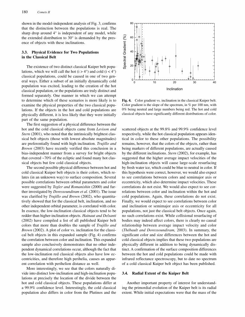
The second possible physical difference between hot andcold classical Kuiper belt objects is their colors, which re-lates (in an unknown way) to surface composition. Severalpossible correlations between orbital parameters and colorwere suggested by Tegler and Romanishin (2000) and fur-ther investigated by Doressoundiram et al. (2001). The issuewas clarified by Trujillo and Brown (2002), who quantita-tively showed that for the classical belt, inclination, and noother independent orbital parameter, is correlated with color.In essence, the low-inclination classical objects tend to beredder than higher-inclination objects. Hainaut and Delsanti(2002) have compiled a list of all published Kuiper beltcolors that more than doubles the sample of Trujillo andBrown (2002). A plot of color vs. inclination for the classi-cal belt objects in this expanded sample (Fig. 4) confirmsthe correlation between color and inclination. This expandedsample also conclusively demonstrates that no other inde-pendent dynamical correlations occur, although the fact thatthe low-inclination red classical objects also have low ec-centricities, and therefore high perihelia, causes an appar-ent correlation with perihelion distance as well.

More interestingly, we see that the colors naturally di-vide into distinct low-inclination and high-inclination popu-lations at precisely the location of the divide between thehot and cold classical objects. These populations differ ata 99.9% confidence level. Interestingly, the cold classicalpopulation also differs in color from the Plutinos and the

scattered objects at the 99.8% and 99.9% confidence levelrespectively, while the hot classical population appears iden-tical in color to these other populations. The possibilityremains, however, that the colors of the objects, rather thanbeing markers of different populations, are actually causedby the different inclinations. Stern (2002), for example, hassuggested that the higher average impact velocities of thehigh-inclination objects will cause large-scale resurfacingby fresh water ice, which could be blue to neutral in color. Ifthis hypothesis were correct, however, we would also expectto see correlations between colors and semimajor axis oreccentricity, which also determine impact velocities. Thesecorrelations do not exist. We would also expect to see cor-relations between color and inclination within the hot andcold populations. Again, these correlations do not exist.Finally, we would expect to see correlations between colorand inclination or semimajor axis or eccentricity for allpopulations, not just the classical belt objects. Once again,no such correlations exist. While collisional resurfacing ofbodies may indeed affect colors, there is clearly no causalrelationship between average impact velocity and color(Thébault and Doressoundiram, 2003). In summary, thesignificant color and size differences between the hot andcold classical objects implies that these two populations arephysically different in addition to being dynamically dis-tinct. A confirmation of the surface composition differencesbetween the hot and cold populations could be made withinfrared reflectance spectroscopy, but to date no spectrumof a cold classical Kuiper belt object has been published.

3.4. Radial Extent of the Kuiper Belt

Another important property of interest for understand-ing the primordial evolution of the Kuiper belt is its radialextent. While initial expectations were that the mass of the

Fig. 4. Color gradient vs. inclination in the classical Kuiper belt.Color gradient is the slope of the spectrum, in % per 100 nm, with0% being neutral and large numbers being red. The hot and coldclassical objects have significantly different distributions of color.

Morbidelli and Brown: Kuiper Belt and Evolution of Solar System 181

Kuiper belt should smoothly decrease with heliocentric dis-tance — or perhaps even increase in number density by afactor of ~100 back to the level of the extrapolation of theminimum mass solar nebula beyond the region of Neptune’sinfluence (Stern, 1996) — the lack of detection of objectsbeyond about 50 AU soon began to suggest a dropoff innumber density (Dones, 1997; Jewitt et al., 1998; Chiangand Brown, 1999; Trujillo et al., 2001; Allen et al., 2001).It was often argued that this lack of detections was the con-sequence of a simple observational bias caused by the ex-treme faintness of objects at greater distances from the Sun(Gladman et al., 1998), but Allen et al. (2001, 2002) showedconvincingly that for a fixed absolute magnitude, the num-ber of objects with semimajor axis <50 AU was larger thanthe number >50 AU and thus some density decrease waspresent.

Determination of the magnitude of the density drop be-yond 50 AU was hampered by the small numbers of ob-jects and thus weak statistics in individual surveys. Trujilloand Brown (2001) developed a method to use all detectedobjects to estimate a radial distribution of the Kuiper belt.The method relies on the fact that the heliocentric distance(not semimajor axis) of objects, like the inclination, is welldetermined in a small number of observations, and thatwithin ~100 AU surveys have no biases against discover-ing distant objects other than the intrinsic radial distribu-tion and the easily quantifiable brightness decrease withdistance. Thus, at a particular distance, a magnitude m0 willcorrespond to a particular object size s, but, assuming apower-law differential size distribution, each detection ofan object of size s can be converted to an equivalent numbern of objects of size s0 by n = (s/s0)q – 1 where q is the differ-ential power-law size index. Thus the observed radial distri-bution of objects with magnitude m0, O(r,m0)dr can be con-verted to the true radial distribution of objects of size s0 by

1q

0

5/)55.24m(

00 s60.15

10)1r(rdr)m,r(Odr)s,r(R

−−−=

where albedos of 4% are assumed, but only apply as a scal-ing factor. Measured values of q for the Kuiper belt haveranged from 3.5 to 4.8 (for a review, see Trujillo and Brown,2001). We will assume the steepest currently proposed valueof q = 4.45 (Gladman et al., 2001), which puts the strongestconstraints on the existence of distant objects.

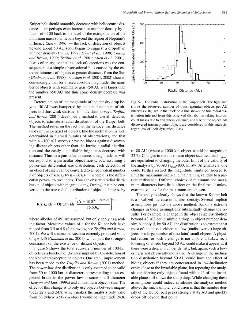
Figure 5 shows the total equivalent number of 100-kmobjects as a function of distance implied by the detection ofthe known transneptunian objects. One small improvementhas been made to the Trujillo and Brown (2001) method.The power-law size distribution is only assumed to be validfrom 50 to 1000 km in diameter, corresponding to an ex-pected break in the power law at some small diameter(Kenyon and Luu, 1999a) and a maximum object’s size. Theeffect of this change is to only use objects between magni-tudes 22.7 and 24.8, which makes the analysis only validfrom 30 (where a 50-km object would be magnitude 24.8)

to 80 AU (where a 1000-km object would be magnitude22.7). Changes in the maximum object size assumed, smax,are equivalent to changing the outer limit of the validity ofthe analysis by 80 AU (smax/1000 km)1/2. Alternatively, onecould further restrict the magnitude limits considered tolimit the maximum size while maintaining validity to a par-ticular distance. Different choices of minimum and maxi-mum diameters have little effect on the final result unlessextreme values for the maximum are chosen.

The analysis clearly shows that the known Kuiper beltis a localized increase in number density. Several implicitassumptions go into the above method, but only extremechanges in these assumptions substantially change the re-sults. For example, a change in the object size distributionbeyond 43 AU could mimic a drop in object number den-sity, but only if, by 50 AU, the distribution is so extreme thatmost of the mass is either in a few (undiscovered) large ob-jects or a large number of (too faint) small objects. A physi-cal reason for such a change is not apparent. Likewise, alowering of albedo beyond 50 AU could make it appear as ifthere were a drop in number density, but, again, such a low-ering is not physically motivated. A change in the inclina-tion distribution beyond 50 AU could have the effect ofhiding objects if they are concentrated in low-inclinationorbits close to the invariable plane, but repeating the analy-sis considering only objects found within 1° of the invari-able plane still shows the sharp drop. While changing theseassumptions could indeed invalidate the analysis methodabove, the much simpler conclusion is that the number den-sity of the Kuiper belt peaks strongly at 42 AU and quicklydrops off beyond that point.

Fig. 5. The radial distribution of the Kuiper belt. The light lineshows the observed number of transneptunian objects per AUinterval (× 10), while the thick bold line shows the true radial dis-tribution inferred from this observed distribution taking into ac-count biases due to brightness, distance, and size of the object. Alldiscovered transneptunian objects are considered in this analysis,regardless of their dynamical class.

182 Comets II

While the Trujillo and Brown (2001) method is good atgiving an indication of the radial structure of the Kuiperbelt where objects have been found, it is less useful fordetermining upper limits to the detection of objects wherenone have been found. A simple extension, however, allowsus to easily test hypothetical radial distributions against theknown observations by looking at observed radial distribu-tions of all objects found at a particular magnitude m0 in-dependent of any knowledge of how these objects werefound. Assume a true radial distribution of objects R(r)drand again assume the above power law differential size dis-tribution and maximum size. For magnitudes between m andm + dm, we can construct the expected observed radial distri-bution of all objects found at that magnitude, o(r,m)drdm, by

dms6.15

10)1r(rdr)r(Rdrdm)m,r(o

1q

0

5/)55.24m( +−−−=

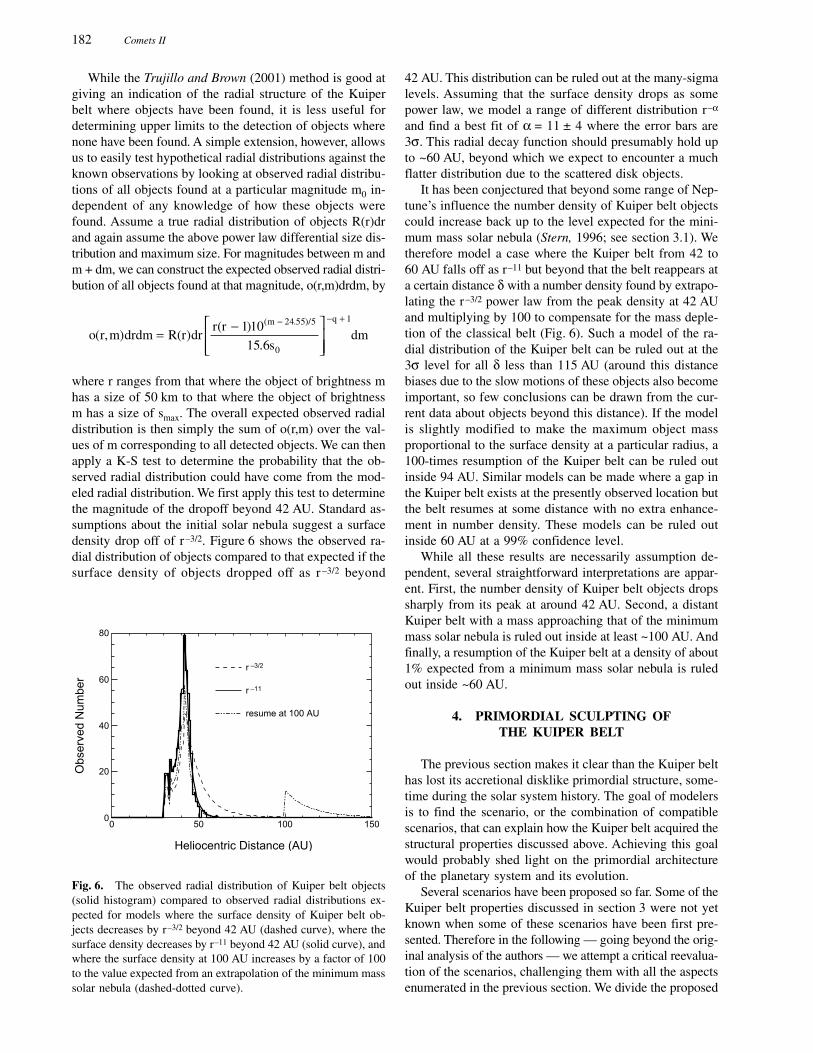
where r ranges from that where the object of brightness mhas a size of 50 km to that where the object of brightnessm has a size of smax. The overall expected observed radialdistribution is then simply the sum of o(r,m) over the val-ues of m corresponding to all detected objects. We can thenapply a K-S test to determine the probability that the ob-served radial distribution could have come from the mod-eled radial distribution. We first apply this test to determinethe magnitude of the dropoff beyond 42 AU. Standard as-sumptions about the initial solar nebula suggest a surfacedensity drop off of r–3/2. Figure 6 shows the observed ra-dial distribution of objects compared to that expected if thesurface density of objects dropped off as r –3/2 beyond

42 AU. This distribution can be ruled out at the many-sigmalevels. Assuming that the surface density drops as somepower law, we model a range of different distribution r–α

and find a best fit of α = 11 ± 4 where the error bars are3σ. This radial decay function should presumably hold upto ~60 AU, beyond which we expect to encounter a muchflatter distribution due to the scattered disk objects.

It has been conjectured that beyond some range of Nep-tune’s influence the number density of Kuiper belt objectscould increase back up to the level expected for the mini-mum mass solar nebula (Stern, 1996; see section 3.1). Wetherefore model a case where the Kuiper belt from 42 to60 AU falls off as r–11 but beyond that the belt reappears ata certain distance δ with a number density found by extrapo-lating the r–3/2 power law from the peak density at 42 AUand multiplying by 100 to compensate for the mass deple-tion of the classical belt (Fig. 6). Such a model of the ra-dial distribution of the Kuiper belt can be ruled out at the3σ level for all δ less than 115 AU (around this distancebiases due to the slow motions of these objects also becomeimportant, so few conclusions can be drawn from the cur-rent data about objects beyond this distance). If the modelis slightly modified to make the maximum object massproportional to the surface density at a particular radius, a100-times resumption of the Kuiper belt can be ruled outinside 94 AU. Similar models can be made where a gap inthe Kuiper belt exists at the presently observed location butthe belt resumes at some distance with no extra enhance-ment in number density. These models can be ruled outinside 60 AU at a 99% confidence level.

While all these results are necessarily assumption de-pendent, several straightforward interpretations are appar-ent. First, the number density of Kuiper belt objects dropssharply from its peak at around 42 AU. Second, a distantKuiper belt with a mass approaching that of the minimummass solar nebula is ruled out inside at least ~100 AU. Andfinally, a resumption of the Kuiper belt at a density of about1% expected from a minimum mass solar nebula is ruledout inside ~60 AU.

4. PRIMORDIAL SCULPTING OFTHE KUIPER BELT

The previous section makes it clear than the Kuiper belthas lost its accretional disklike primordial structure, some-time during the solar system history. The goal of modelersis to find the scenario, or the combination of compatiblescenarios, that can explain how the Kuiper belt acquired thestructural properties discussed above. Achieving this goalwould probably shed light on the primordial architectureof the planetary system and its evolution.

Several scenarios have been proposed so far. Some of theKuiper belt properties discussed in section 3 were not yetknown when some of these scenarios have been first pre-sented. Therefore in the following — going beyond the orig-inal analysis of the authors — we attempt a critical reevalua-tion of the scenarios, challenging them with all the aspectsenumerated in the previous section. We divide the proposed

Fig. 6. The observed radial distribution of Kuiper belt objects(solid histogram) compared to observed radial distributions ex-pected for models where the surface density of Kuiper belt ob-jects decreases by r–3/2 beyond 42 AU (dashed curve), where thesurface density decreases by r–11 beyond 42 AU (solid curve), andwhere the surface density at 100 AU increases by a factor of 100to the value expected from an extrapolation of the minimum masssolar nebula (dashed-dotted curve).

Morbidelli and Brown: Kuiper Belt and Evolution of Solar System 183

scenarios in three groups: (1) those invoking sweeping reso-nances, which offer a view of gentle evolution of the pri-mordial solar system; (2) those invoking the action of mas-sive scatterers (lost planets or passing stars), which offeran opposite view of violent and chaotic primordial evolu-tion; and (3) those aimed at building the Kuiper belt as thesuperposition of two populations with distinctive dynamicalhistories, somehow combining the scenarios in groups (1)and (2).

4.1. Resonance Sweeping Scenarios

Fernández and Ip (1984) showed that, while scatteringprimordial planetesimals, Neptune should have migrated

outward. Malhotra (1993, 1995) realized that, followingNeptune’s migration, the mean-motion resonances withNeptune also migrated outward, sweeping the primordialKuiper belt until they reached their present position. Fromadiabatic theory (Henrard, 1982), most of the Kuiper beltobjects swept by a mean-motion resonance would have beencaptured into resonance; they would have subsequentlyfollowed the resonance in its migration, while increasingtheir eccentricity. This model accounts for the existence ofthe large number of Kuiper belt objects in the 2:3 mean-motion resonance with Neptune (and also in other reso-nances) and explains their large eccentricities (see Fig. 7).Reproducing the observed range of eccentricities of theresonant bodies requires that Neptune migrated by 7 AU.

Fig. 7. Final distribution of the Kuiper belt bodies according to the sweeping resonances scenario (courtesy of R. Malhotra). Thesimulation is done by numerical integrating, over a 200-m.y. timespan, the evolution of 800 test particles on initial quasicircular andcoplanar orbits. The planets are forced to migrate (Jupiter: –0.2 AU; Saturn: 0.8 AU; Uranus: 3 AU; Neptune: 7 AU) and reach theircurrent orbits on an exponential timescale of 4 m.y. Large solid dots represent “surviving” particles (i.e., those that have not sufferedany planetary close encounters during the integration time); small dots represent the “removed” particles at the time of their closeencounter with a planet. In the lowest panel, the solid line is the histogram of semimajor axis of the “surviving” particles; the dottedline is the initial distribution.

184 Comets II

Malhotra’s (1993, 1995) simulations also showed that thebodies captured in the 2:3 resonance can acquire large in-clinations, comparable to that of Pluto and other objects.The mechanisms that excite the inclination during the cap-ture process have been investigated in detail by Gomes(2000). The author concluded that, although large inclina-tions can be achieved, the resulting proportion between thenumber of high-inclination vs. low-inclination bodies andtheir distribution in the eccentricity vs. inclination plane donot reproduce the observations very well.

The mechanism of adiabatic capture into resonance re-quires that Neptune’s migration happened very smoothly.If Neptune had encountered a significant number of largebodies (1 M or more), its jerky migration would have jeop-ardized capture into resonances. Hahn and Malhotra (1999),who simulated Neptune’s migration using a disk of lunar-to martian-mass planetesimals, did not obtain any perma-nent capture. The precise constraints set by the capture proc-ess on the size distribution of the largest disk’s planetesimalshave never been quantitatively computed, but they are likelyto be severe.

In the mean-motion resonance sweeping model the ec-centricities and inclinations of the nonresonant bodies arealso excited by the passage of many weak resonances, butthe excitation that does occur is too small to account forthose observed (compare Fig. 7 with Fig. 1). Some othermechanism (like those discussed below) must also haveacted to produce the observed overall orbital excitation ofthe Kuiper belt. The question of whether this other mecha-nism acted before or after the resonance sweeping and cap-ture process is unresolved. Had it occurred afterward, itwould have probably ejected most of the previously cap-tured objects from the resonances (not necessarily a prob-lem if the number of captured bodies was large enough).Had it happened before, then the mean-motion resonanceswould have had to capture particles from an excited disk.Another long-debated question concerning the sweepingmodel is the relative proportion between the number ofbodies in the 2:3 and 1:2 resonances. The original simula-tions by Malhotra indicated that the population in the 1:2resonance should be comparable to — if not greater than —that in the 2:3 resonance. This prediction seemed to be inconflict with the absence of observed bodies in the formerresonance at that time. Ida et al. (2000a) showed that theproportion between the two populations is very sensitive toNeptune’s migration rate and that the small number of 1:2resonant bodies, suggested by the lack of observations,would just be indicative of a fast migration (105–106 yrtimescale). Since then, five objects have been discoveredin or close to the 1:2 resonance (given orbital uncertaintiesit is not yet possible to guarantee that all of them are reallyinside the resonance). There is no general consensus on thedebiased ratio between the populations in the 2:3 and 1:2resonances, because the debiasing is necessarily model-dependent and the current data on the population of the 1:2resonance are sparse. Trujillo et al. (2001) estimated a 2:3to 1:2 ratio close to 1/2, while Chiang and Jordan (2002)

obtained a ratio closer to 3. Chiang and Jordan (2002) alsonoted that the positions of the five potential 1:2 resonantobjects are unusually located with respect to a referenceframe rotating with Neptune, which may also have impli-cations for migration rates and capture mechanisms.

The migration of secular resonances could also have con-tributed to the excitation of the eccentricities and inclina-tions of Kuiper belt bodies. Secular resonances occur whenthe precession rates of the orbits of the bodies are in simpleratio with the precession rates of the orbits of the planets.There are several reasons to think that secular resonancescould have been in different locations in the past and mi-grated to their current location at about 40–42 AU. A grad-ual mass loss of the belt due to collisional activity, thegrowth of Neptune’s mass, and Neptune’s orbital migrationwould have moved the secular resonance with Neptune’sperihelion outward. Levison et al. (personal communication,1997) found that the Kuiper belt interior to 42 AU wouldhave suffered a strong eccentricity excitation. However, thequantitative simulations show that the orbital distributionof the surviving bodies in the 2:3 resonance would not besimilar to the observed one: The eccentricities of mostsimulated bodies would range between 0.05 and 0.1, whilethose of the observed Plutinos are between 0.1 and 0.3.Also, in this model there is basically no eccentricity andinclination excitation for the Kuiper belt bodies with a >42 AU, in contrast with what is observed.

The dissipation of the primordial nebula would also havecaused the migration of the secular resonances. Nagasawaand Ida (2000) showed that the secular resonances involv-ing the precession rates of the perihelion longitudes wouldhave migrated from beyond 50 AU to their current positionduring the nebula dispersion. This could have caused ec-centricity excitation of the Kuiper belt in the 40–50 AU re-gion. In addition, if the midplane of the nebula was notorthogonal to the total angular momentum vector of theplanetary system, a secular resonance involving the preces-sion rates of the node longitudes would also have swept theKuiper belt, causing inclination excitation. The magnitudeof the eccentricity and inclination excitation depends on thetimescale of the nebula dissipation. A dissipation timescaleof ~107 yr is required in order to excite the eccentricitiesup to 0.2–0.3 and the inclinations up to 20°–30°. But if Nep-tune was at about 20 AU at the time of the nebula disappear-ance — as required by the mean-motion resonance sweep-ing model — the disspation timescale should have been~108 yr, suspiciously lengthy with respect to what is ex-pected from current theories and observations on the evolu-tion of protoplanetary disks. A major failure of the modelis that, because only one nodal secular resonance sweepsthe belt, all the Kuiper belt bodies acquire orbits with com-parably large inclinations. In other words, the model doesnot reproduce the observed spread of inclinations, nor theirbimodal distribution. No correlation between inclination andsize or color can be explained either. The same is not truefor the eccentricities, because the belt is swept by severalperihelion resonances, which causes a spread in the final

Morbidelli and Brown: Kuiper Belt and Evolution of Solar System 185

values. The secular resonance sweeping model cannot ex-plain the existence of significant populations in mean-mo-tion resonances, so that the mean-motion resonance sweep-ing model would still need to be invoked.

None of the models discussed above can explain theexistence of the edge of the belt at ~50 AU.

4.2. Scattering Scenarios

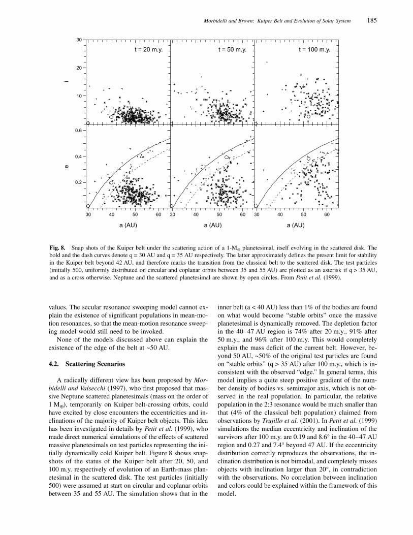
A radically different view has been proposed by Mor-bidelli and Valsecchi (1997), who first proposed that mas-sive Neptune scattered planetesimals (mass on the order of1 M ), temporarily on Kuiper belt-crossing orbits, couldhave excited by close encounters the eccentricities and in-clinations of the majority of Kuiper belt objects. This ideahas been investigated in details by Petit et al. (1999), whomade direct numerical simulations of the effects of scatteredmassive planetesimals on test particles representing the ini-tially dynamically cold Kuiper belt. Figure 8 shows snap-shots of the status of the Kuiper belt after 20, 50, and100 m.y. respectively of evolution of an Earth-mass plan-etesimal in the scattered disk. The test particles (initially500) were assumed at start on circular and coplanar orbitsbetween 35 and 55 AU. The simulation shows that in the

inner belt (a < 40 AU) less than 1% of the bodies are foundon what would become “stable orbits” once the massiveplanetesimal is dynamically removed. The depletion factorin the 40–47 AU region is 74% after 20 m.y., 91% after50 m.y., and 96% after 100 m.y. This would completelyexplain the mass deficit of the current belt. However, be-yond 50 AU, ~50% of the original test particles are foundon “stable orbits” (q > 35 AU) after 100 m.y., which is in-consistent with the observed “edge.” In general terms, thismodel implies a quite steep positive gradient of the num-ber density of bodies vs. semimajor axis, which is not ob-served in the real population. In particular, the relativepopulation in the 2:3 resonance would be much smaller thanthat (4% of the classical belt population) claimed fromobservations by Trujillo et al. (2001). In Petit et al. (1999)simulations the median eccentricity and inclination of thesurvivors after 100 m.y. are 0.19 and 8.6° in the 40–47 AUregion and 0.27 and 7.4° beyond 47 AU. If the eccentricitydistribution correctly reproduces the observations, the in-clination distribution is not bimodal, and completely missesobjects with inclination larger than 20°, in contradictionwith the observations. No correlation between inclinationand colors could be explained within the framework of thismodel.

Fig. 8. Snap shots of the Kuiper belt under the scattering action of a 1-M planetesimal, itself evolving in the scattered disk. Thebold and the dash curves denote q = 30 AU and q = 35 AU respectively. The latter approximately defines the present limit for stabilityin the Kuiper belt beyond 42 AU, and therefore marks the transition from the classical belt to the scattered disk. The test particles(initially 500, uniformly distributed on circular and coplanar orbits between 35 and 55 AU) are plotted as an asterisk if q > 35 AU,and as a cross otherwise. Neptune and the scattered planetesimal are shown by open circles. From Petit et al. (1999).

186 Comets II

A variant of the Petit et al. scenario has been invokedby Brunini and Melita (2002) to explain the apparent edgeof the Kuiper belt at 50 AU. They showed with numericalsimulations that a Mars-sized body residing for 1 G.y. onan orbit with a ~ 60 AU and e ~ 0.15–0.2 could have scat-tered into Neptune-crossing orbits most of the Kuiper beltbodies originally in the 50–70 AU range, leaving this re-gion strongly depleted and dynamically excited. Such amassive body should have been a former Neptune-scatteredplanetesimal that decoupled from Neptune due to the dy-namical friction exerted by the initially massive Kuiper belt.The orbital distribution inside ~50 AU is not severely af-fected by the massive planetesimal once on its decoupledorbit at a ~ 60 AU (see also Melita et al., 2002). However,a strong dynamical excitation could be obtained during thetransfer phase, when the massive planetesimal was trans-ported by Neptune encounters toward a ~ 60 AU, similarto what happens in the Petit et al. (1999) simulations. Someof the simulations by Brunini and Melita (2002) that in-clude this transfer phase lead to an (a, e) distribution thatis perfectly consistent with what is currently observed inthe classical belt in terms of mass depletion, eccentricityexcitation, and outer edge (see, e.g., their Fig. 10). Thecorresponding inclination distribution is not explicitely dis-cussed, but it is less excited than in the Petit et al. (1999)scenario (M. Melita, personal communication, 2002). Simi-larly, a correlation between inclination and size or colorcannot be reproduced by this mechanism, and a distinctivePlutino population is not formed. Finally, our numericalsimulations show that a 1-M planet in the Kuiper beltcannot transport bodies up to 200 AU or more by gravita-tional scattering. Therefore, neither the Petit et al. (1999)scenario nor that of Brunini and Melita (2002) can explainthe origin of the orbit of objects such as 2000 CR105.

A potential problem of the Brunini and Melita scenariois that, once the massive body is decoupled from Neptune,there are no evident dynamical mechanisms that wouldensure its later removal from the system. In other words,the massive body should still be present, somewhere in the~50–70-AU region. A Mars-sized body with 4% albedo at70 AU would have apparent magnitude brighter than 20, sothat, if its inclination is small (i < 10°), as expected if thebody got trapped in the Kuiper belt by dynamical friction,it is unlikely that it escaped detection in the numerous wide-field ecliptic surveys that have been performed up to now,and in particular in that led by Trujillo and Brown (2003).

Another severe problem, for both the Petit et al. (1999)and Brunini and Melita (2002) scenarios — as well as forany other scenario that attempts to explain the mass deple-tion of the Kuiper belt by the dynamical ejection of a sub-stantial fraction of Kuiper belt bodies to Neptune-crossingorbit — is that Neptune would have migrated well beyond30 AU. In Hahn and Malhotra (1999) simulations, a 50 Mdisk between 10 and 60 AU drives Neptune to ~30 AU. Inthis process, Neptune interacts only with the mass in the10–35-AU disk (about 25 M ), and a massive Kuiper beltremains beyond Neptune. But if the Kuiper belt had been

excited to Neptune-crossing orbit, then Neptune would haveinteracted with the full 50-M disk and therefore wouldhave migrated much further. [This fact was not noticed bythe simulations of Petit et al. (1999) and Brunini and Melita(2002), because the former considered a Kuiper belt ofmassless particles and the latter a Kuiper belt whose totalmass was only ~1 M .] To limit Neptune’s migration at30 AU, the total mass of the disk, including the Kuiper belt,should have been significantly smaller. Our simulationsshow that even a disk of 15 M between 10 and 50 AU,once excited to Neptune-crossing orbit, would drive Nep-tune too far. Therefore, the scenario of a massive body scat-tered by Neptune through the Kuiper belt is viable only ifthe primordial mass of the belt was significantly smaller thanusually accepted (accounting only for a few Earth masses).

Motivated by the observation that the eccentricity of theclassical belt bodies on average increases with semimajoraxis (a fact certainly enhanced by the observational biases,which strongly favor the discovery of bodies with smallperihelion distances), Ida et al. (2000b) suggested that thestructure of the classical belt records the footprint of theclose encounter with a passing star. In that paper and in thefollowup work by Kobayashi and Ida (2001), the resultingeccentricities and inclinations were computed as a functionof a/D, where a is the original body’s semimajor axis andD is the heliocentric distance of the stellar encounter, forvarious choices of the stellar parameters (inclination, mass,and eccentricity). The eccentricity distribution in the clas-sical belt suggested to the authors a stellar encounter atabout ~150 AU. The same parameters, however, do not leadto an inclination excitation comparable to the observed one.The latter would require a stellar passage at ~100 AU orless. From Kobayashi and Ida simulations we argue that abimodal inclination distribution could be possibly obtained,but a quantitative fit to the debiased distribution discussedin section 3.2 has never been attempted. A stellar encoun-ter at ~100 AU would make most of the classical belt bod-ies so eccentric to intersect the orbit of Neptune. Therefore,it would explain not only the dynamical excitation of thebelt (although a quantitative comparison with the observeddistributions has never been done) but also its mass deple-tion, but would encounter the same problem discussed aboutconcerning Neptune’s migration.

Melita et al. (2002) showed that a stellar passage at about200 AU would be sufficient to explain the edge of the clas-sical belt at 50 AU. An interesting constraint on the time atwhich such an encounter occurred is set by the existenceof the Oort cloud. Levison et al. (2003) show that the en-counter had to occur much earlier than ~10 m.y. after theformation of Uranus and Neptune, otherwise most of theexisting Oort cloud would have been ejected to interstellarspace and many of the planetesimals in the scattered diskwould have had their perihelion distance lifted beyond Nep-tune, decoupling from the planet. As a consequence, the ex-tended scattered disk population, with a > 50 AU and 40 <q < 50 AU, would have had a mass comparable or largerthan that of the resulting Oort cloud, hardly compatible with

Morbidelli and Brown: Kuiper Belt and Evolution of Solar System 187

the few detections of extended scattered disk objects per-formed up to now. An encounter with a star during the firstmillion years from planetary formation is a likely event ifthe Sun formed in a stellar cluster (Bate et al., 2003). Atsuch an early time, presumably the Kuiper belt objects werenot yet fully formed (Stern, 1996; Kenyon and Luu, 1998).In this case, the edge of the belt would be at a heliocentricdistance corresponding to a postencounter eccentricity ex-citation of ~0.05, a threshold value below which collisionaldamping is efficient and accretion can recover, and beyondwhich the objects rapidly grind down to dust (Kenyon andBromley, 2002). The edge-forming stellar encounter couldnot be responsible for the origin of the peculiar orbit of2000 CR105. In fact, such a close encounter would also pro-duce a relative overabundance of bodies with perihelion dis-tance similar to that of 2000 CR105 but with semimajor axisin the 50–200-AU range. These bodies have never been dis-covered despite the more favorable observational biases. Inorder that only bodies with a > 200 AU have their perihe-lion distance lifted, a second stellar passage at about 800 AUis required (Morbidelli and Levison, 2003). Interestingly,from the analysis of the Hipparcos data, Garcia-Sanchezet al. (2001) concluded that, with the current stellar envi-ronment, the closest encounter with a star during the ageof the solar system would be at ~900 AU.

4.3. Scenarios for a Two-Component Kuiper Belt

None of the scenarios discussed above successfully re-produce the existence of a cold and a hot population in theclassical belt (see section 3.2–3.3) and the correlation be-tween inclination and sizes and colors. The reason is obvi-ous. All these scenarios start with a unique population (theprimordial, dynamically cold Kuiper belt). From a uniquepopulation, it is very difficult to produce two populationswith distinct orbital properties. Even in the case where itmight be possible (as in the stellar encounter scenario), theorbital histories of gray bodies cannot differ statisticallyfrom those of the red bodies, because the dynamics do notdepend on the physical properties. The correlations betweencolors and inclination can be explained only by postulat-ing that the hot and cold populations of the current Kuiperbelt originally formed in distinctive places in the solar sys-tem. The scenario suggested by Levison and Stern (2001)is that initially the protoplanetary disk in the Uranus-Nep-tune region and beyond was uniformly dynamically cold,with physical properties that varied with heliocentric dis-tance. Then, a dynamical violent event cleared the innerregion of the disk, dynamically scattering the inner diskobjects outward. In the scattering process, large inclinationswere acquired. Most of these objects have been dynami-cally eliminated, or persist as members of the scattered disk.However, a few of these objects somehow were depositedin the main Kuiper belt, becoming the hot population of theclassical belt currently observed.

Two dynamical scenarios have been proposed so far toexplain how planetesimals in the Uranus-Neptune zone

could be permanently trapped in the Kuiper belt. Thommeset al. (1999) proposed a radical view of the primordial ar-chitecture of our outer solar system in which Uranus andNeptune formed in the Jupiter-Saturn zone. In their simu-lations, Uranus and Neptune were rapidly scattered outwardby Jupiter, where the interaction with the massive disk ofplanetesimals damped their eccentricities and inclinationsby dynamical friction; as a consequence, the planets escapedfrom the scattering action of Jupiter before ejection on hy-perbolic orbit could occur. In about 50% of the cases, thefinal states resembled the current structure of the outer solarsystem, with four planets roughly at the correct locations.In this scenario Neptune experienced a high-eccentricityphase lasting for a few million years, during which its aph-elion distance was larger than the current one. The planetesi-mals scattered by Neptune during the dynamical frictionprocess therefore formed a scattered disk that extended wellbeyond its current perihelion distance boundary. When Nep-tune’s eccentricity decreased down to its present value, thelarge-q part of the scattered disk became “fossilized,” be-ing unable to closely interact with Neptune again. This sce-nario therefore explains how a population of bodies, origi-nally formed in the inner part of the disk, could be trappedin the classical belt. However, the inclination excitation ofthis population, although relevant, is smaller than that ofthe observed hot population. This is probably due to the factthat Neptune’s eccentricity is rapidly damped, so that theparticles undergo Neptune’s scattering action for only a fewmillion years, too short a timescale to acquire large incli-nations. For the same reason, the “fossilized” scattered diskdoes not extend very far in semimajor axis, so that objectslike 2000 CR105 are not produced in this scenario. Also, thehigh eccentricity of Neptune would destabilize the bodiesin the 2:3 resonance, so that the Plutinos could have beencaptured only after Neptune’s eccentricity damping, duringa final quiescent phase of radial migration similar to thatin Malhotra’s (1993, 1995) scenario. Nevertheless, a Plutinopopulation was never formed in the Thommes et al. (1999)simulations, possibly because Neptune’s migration was toojerky owing to the encounters with the massive bodies usedin the numerical representation of the disk.

Gomes (2003) revisited Malhotra’s (1993, 1995) model.Like Hahn and Malhotra (1999), he attempted to simulateNeptune’s migration, starting from about 15 AU, by theinteraction with a massive planetesimal disk extending frombeyond Neptune’s initial position. But, taking advantage ofthe improved computer technology, he used 10,000 particlesto simulate the disk population, with individual massesroughly equal to twice the mass of Pluto, while Hahn andMalhotra used only 1000 particles with lunar to martianmasses. In his simulations, during its migration Neptunescattered the planetesimals and formed a massive scattereddisk. Some of the scattered bodies decoupled from theplanet by decreasing their eccentricity through the interac-tion with some secular or mean-motion resonance. If Nep-tune had not been migrating, as in Duncan and Levison(1997) integrations, the decoupled phases would have been

188 Comets II

transient, because the eccentricity would have eventuallyincreased back to Neptune-crossing values, the dynamicsbeing reversible. But Neptune’s migration broke the reversi-bility, and some of the decoupled bodies managed to escapefrom the resonances, and remained permanently trapped inthe Kuiper belt. As shown in Fig. 9, the current Kuiper beltwould therefore be the result of the superposition of thesebodies with the local population, originally formed beyond30 AU and only moderately excited [by the resonance sweep-ing mechanism, as in Hahn and Malhotra (1999)]. Unlikein Thommes et al. (1999) simulations, the migration mecha-nism is sufficiently slow (several 107 yr) that the scatteredparticles have the time to acquire very large inclinations,consistent with the observed hot population. The resultinginclination distribution of the bodies in the classical belt isbimodal, and quantitatively reproduces the debiased inclina-tion distribution computed by Brown (2001) from the obser-vations. For the same reason (longer timescale) the extendedscattered disk in Gomes’ (2003) simulations reaches muchlarger semimajor axes than in Thommes et al. (1999) inte-grations. Although bodies on orbits similar to that of 2000CR105 are not obtained in the nominal simulations, othertests done in Gomes (2003) are suggestive that such orbitscould be achieved in the framework of the same scenario.

A significant Plutino population is also created in Gomes’simulations. This population is also the result of the super-position of the population coming from Neptune’s regionwith that formed further away and captured by the 2:3 reso-nance during the sweeping process. Assuming that the bod-ies’ sizes and colors varied in the primordial disk withheliocentric distance, this process would explain why thePlutinos, scattered objects, and hot classical belt objects,which mostly come from regions inside ~30 AU, all appearto have identical color distributions and similar maximumsizes, while only the cold classical population, the only ob-jects actually formed in the transneptunian region, has a dif-ferent distribution in color and size.

Of all the models discussed in this paper, Gomes’ sce-nario is the one that seems to best account for the observedproperties of the classical belt. A few open questions persist,though. The first concerns the mass deficit of the Kuiperbelt. In Gomes’ simulations about 0.2% of the bodies ini-tially in the Neptune-swept disk remained in the Kuiper beltat the end of Neptune’s migration. Assuming that the pri-mordial disk was ~100 M , this is very compatible with theestimated current mass of the Kuiper belt. But the localpopulation was only moderately excited and not dynami-cally depleted, so it should have preserved most of its pri-mordial mass. The latter should have been several Earthmasses, in order to allow the growth of ~100-km bodieswithin a reasonable timescale (Stern, 1996). How did thislocal population lose its mass? This problem is also unre-solved for the Thommes et al. (1999) scenario. The onlyplausible answer seems to be the collisional erosion sce-nario, but it has the limitations discussed in section 3.1.Quantitative simulations need to be done. A second prob-lem, also common to the Thommes et al. scenario, is theexistence of the Kuiper belt edge at 50 AU. In fact, in nei-ther scenario is significant depletion of the pristine popu-lation beyond this threshold obtained. A third problem withGomes’ (2003) scenario concerns Neptune’s migration. Whydid it stop at 30 AU? There is no simple explanation withinthe model, so Gomes had to artificially impose the end ofNeptune’s migration by abruptly dropping the mass surfacedensity of the disk at ~30 AU. A possibility is that, by thetime that Neptune reached that position, the disk beyond30 AU had already been severely depleted by collisions. Asecond possibility is that something (a massive planetaryembryo, a stellar encounter, collisional grinding?) openeda gap in the disk at about 30 AU, so that Neptune ran outof material and could not further sustain its migration.

5. CONCLUSIONS AND PERSPECTIVES

Ten years of dedicated surveys have revealed unexpectedand intriguing properties of the transneptunian population,such as the existence of a large number of bodies trappedin mean-motion resonances, the overall mass deficit, thelarge orbital eccentricities and inclinations, and the appar-ent existence of an outer edge at ~50 AU and a correlationamong inclinations, sizes, and colors. Understanding how

Fig. 9. The orbital distribution in the classical belt according toGomes’ (2003) simulations. The dots denote the local population,which is only moderately dynamically excited. The crosses de-note the bodies that were originally inside 30 AU. Therefore, theresulting Kuiper belt population is the superposition of a dynami-cally cold population and of a dynamically hot population, whichgives a bimodal inclination distribution comparable to that ob-served. The dotted curves in the eccentricity vs. semimajor axisplot correspond to q = 30 AU and q = 35 AU. Courtesy of R.Gomes.

Morbidelli and Brown: Kuiper Belt and Evolution of Solar System 189

the Kuiper belt acquired all these properties would prob-ably constrain several aspects of the formation of the outerplanetary system and of its primordial evolution.

Up to now, a portfolio of scenarios have been proposedby theoreticians. None of them can account for all the ob-servations alone, and the solution of the Kuiper belt primor-dial sculpting problem probably requires a sapient combina-tion of the proposed models. The Malhotra-Gomes scenarioon the effects of planetary migration does a quite good job atreproducing the observed orbital distribution inside 50 AU.The apparent edge of the belt at 50 AU might be explainedby a very early stellar encounter at 150–200 AU. The originof the peculiar orbit of 2000 CR105 could be due to a laterstellar encounter at ~800 AU.

The most mysterious feature that remains unexplainedin this combination of scenarios is the mass deficit of thecold classical belt. As discussed in this chapter, the massdepletion cannot be explained by the ejection of most ofthe pristine bodies to Neptune-crossing orbit, because in thiscase the planet would have migrated well beyond 30 AU.But the collisional grinding scenario also seems problem-atic, because it requires a peculiar size distribution in theprimordial population and relative encounter velocities thatare larger than those that characterize the objects of the coldpopulation; moreover, an intense collisional activity wouldhave hardly preserved the widely separated binaries that arefrequently observed in the current population.

A possible solution to this problem has been recentlyproposed by Levison and Morbidelli (2003). In their sce-nario, the primordial edge of the massive protoplanetarydisk was somewhere around 30–35 AU and the entire Kui-per belt population — not only the hot component as inGomes’ (2003) scenario — formed within this limit and wastransported to its current location during Neptune’s migra-tion. The transport process of the cold population was dif-ferent from the one found by Gomes for the hot population.These bodies were trapped in the 1:2 resonance with Nep-tune and transported outward within the resonance, untilthey were progressively released due to the nonsmoothnessof the planetary migration. In the standard adiabatic migra-tion scenario (Malhotra, 1995) there would be a resultingcorrelation between the eccentricity and the semimajor axisof the released bodies. However, this correlation is brokenby a secular resonance embedded in the 1:2 mean-motionresonance. This secular resonance is generated because theprecession rate of Neptune’s orbit is modified by the torqueexerted by the massive protoplanetary disk that drives themigration. Simulations of this process match the observed(a, e) distribution of the cold population fairly well, whilethe initially small inclinations are only very moderatelyperturbed. In this scenario, the small mass of the currentKuiper belt population is simply due to the fact that pre-sumably only a small fraction of the massive disk popula-tion was initially trapped in the 1:2 resonance and releasedon stable nonresonant orbits. The preservation of the binaryobjects is not a problem because these objects were movedout of the massive disk in which they formed by a gentle

dynamical process. The final position of Neptune wouldsimply reflect the primitive truncation of the protoplanetarydisk. A bigger problem is the explanation of the differentphysical properties of the cold and hot populations, becausethey both originated within 35 AU, although in somewhatdifferent parts of the disk. At the time of this writing, thisinnovative model has not yet been critically debated withinthe community of experts. But this scenario offers a simpleprediction that will be confirmed or denied by future ob-servations: The edge of the cold classical belt is exactly atthe location of the 1:2 resonance.

Kuiper belt science is a rapidly evolving field. New ob-servations change our view of the belt every year. Since thediscovery of the first transneptunian object 10 years ago,several review papers have been written, and most of themare already obsolete. No doubt this will also be the fate ofthis chapter, but it can be hoped that the ideas presentedhere can continue to guide us in the direction of furtherunderstanding of what present observations of the Kuiperbelt can tell us about the formation and evolution of theouter solar system.

REFERENCES

Allen R. L., Bernstein G. M., and Malhotra R. (2001) The edgeof the solar system. Astroph. J. Lett., 549, L241–L244.

Allen R. L., Bernstein G. M., and Malhotra R. (2002) Observa-tional limits on a distant cold Kuiper belt. Astron. J., 124,2949–2954.

Bate M. R., Bonnell I. A., and Bromm V. (2003) The formationof a star cluster: Predicting the properties of stars and browndwarfs. Mon. Not. R. Astron. Soc., 339, 577–599.

Brown M. (2001) The inclination distribution of the Kuiper belt.Astron. J., 121, 2804–2814.

Brunini A. and Melita M. (2002) The existence of a planet be-yond 50 AU and the orbital distribution of the classicalEdgeworth-Kuiper-belt objects. Icarus, 160, 32–43.

Chiang E. I. and Brown M. E. (1999) Keck pencil-beam surveyfor faint Kuiper belt objects. Astron. J., 118, 1411–1422.

Chiang E. I. and Jordan A. B. (2002) On the Plutinos and Twotinosof the Kuiper belt. Astron. J., 124, 3430–3444.

Chiang E. I., Jordan A. B., Millis R. L., Buie M. W., WassermanL. H., Elliot J. L., Kern S. D., Trilling D. E., Meech K. J., andWagner R. M. (2003) Resonance occupation in the Kuiper belt:Case examples of the 5:2 and Trojan resonances. Astron. J.,126, 430–443.

Cohen C. J. and Hubbard E. C. (1965) The orbit of Pluto. TheObservatory, 85, 43–44.

Davis D. R. and Farinella P. (1997) Collisional evolution ofEdgeworth-Kuiper belt objects. Icarus, 125, 50–60.

Davis D. R. and Farinella P. (1998) Collisional erosion of a mas-sive Edgeworth-Kuiper belt: Constraints on the initial popula-tion (abstract). In Lunar and Planetary Science XIX, pp. 1437–1438. Lunar and Planetary Institute, Houston.

Dones L. (1997) Origin and evolution of the Kuiper belt. In FromStardust to Planetesimals (Y. J. Pendleton and A. G. G. M.Tielens, eds.), p. 347. ASP Conference Series 122.

Doressoundiram A., Barucci M. A., Romon J., and Veillet C.(2001) Multicolor photometry of trans-Neptunian objects.Icarus, 154, 277–286.

190 Comets II

Duncan M. J. and Levison H. F. (1997) Scattered comet disk andthe origin of Jupiter family comets. Science, 276, 1670–1672.

Duncan M. J., Levison H. F., and Budd S. M. (1995) The long-term stability of orbits in the Kuiper belt. Astron. J., 110, 3073–3083.

Farinella P., Davis D. R., and Stern S. A. (2000) Formation andcollisional evolution of the Edgeworth-Kuiper belt. In Proto-stars and Planets IV (V. Mannings et al., eds.), pp. 125–133.Univ. of Arizona, Tucson.

Fernández J. A. and Ip W. H. (1984) Some dynamical aspects ofthe accretion of Uranus and Neptune — The exchange of or-bital angular momentum with planetesimals. Icarus, 58, 109–120.

Garcia-Sanchez J., Weissman P. R., Preston R. A., Jones D. L.,Lestrade J. F., Latham D. W., Stefanik R. P., and Paredes J. M.(2001) Stellar encounters with the solar system. Astron. Astro-phys., 379, 634–659.

Gladman B., Kavelaars J. J., Nicholson P. D., Loredo T. J., andBurns J. A. (1998) Pencil-beam surveys for faint trans-Neptu-nian objects. Astron. J., 116, 2042–2054.

Gladman B., Kavelaars J. J., Petit J. M., Morbidelli A., HolmanM. J., and Loredo Y. (2001) The structure of the Kuiper belt:Size distribution and radial extent. Astron. J., 122, 1051–1066.

Gladman B., Holman M., Grav T., Kaavelars J. J., Nicholson P.,Aksnes K., and Petit J. M. (2002) Evidence for an extendedscattered disk. Icarus, 157, 269–279.

Goldreich P., Lithwick Y., and Sari R. (2002) Formation of Kuiper-belt binaries by dynamical friction and three-body encounters.Nature, 420, 643–646.

Gomes R. S. (2000) Planetary migration and Plutino orbital incli-nations. Astron. J., 120, 2695–2707.

Gomes R. S. (2003) The origin of the Kuiper belt high inclina-tion population. Icarus, 161, 404–418.

Hahn J. M. and Malhotra R. (1999) Orbital evolution of planetsembedded in a planetesimal disk. Astron. J., 117, 3041–3053.

Hainaut O. and Delsanti A. (2002) MBOSS Magnitude and Colors.Available on line at http://www.sc.eso.org/~ohainaut/MBOSS/.

Henrard J. (1982) Capture into resonance — An extension of theuse of adiabatic invariants. Cel. Mech., 27, 3–22.

Ida S., Bryden G., Lin D. N., and Tanaka H. (2000a) Orbitalmigration of Neptune and orbital distribution of trans-Neptu-nian objects. Astrophys. J., 534, 428–445.

Ida S., Larwood J., and Burkert A. (2000b) Evidence for earlystellar encounters in the orbital distribution of Edgeworth-Kuiper belt objects. Astrophys. J., 528, 351–356.

Jewitt D. C. and Luu J. X. (1993) Discovery of the candidateKuiper belt object 1992 QB1. Nature, 362, 730–732.

Jewitt D., Luu J., and Chen J. (1996) The Mauna-Kea-Cerro-Totlolo (MKCT) Kuiper belt and Centaur survey. Astron. J.,112, 1225–1232.

Jewitt D., Luu J., and Trujillo C. (1998) Large Kuiper belt ob-jects: The Mauna Kea 8K CCD survey. Astron. J., 115, 2125–2135.

Kenyon S. J. and Luu J. X. (1998) Accretion in the early Kuiperbelt: I. Coagulation and velocity evolution. Astron. J., 115,2136–2160.

Kenyon S. J. and Luu J. X. (1999a) Accretion in the early Kuiperbelt: II. Fragmentation. Astron. J., 118, 1101–1119.

Kenyon S. J. and Luu J. X. (1999b) Accretion in the early outersolar system. Astrophys. J., 526, 465–470.

Kenyon S. J. and Bromley B. C. (2002) Collisional cascades inplanetesimal disks. I. Stellar flybys. Astron. J., 123, 1757–1775.

Kobayashi H. and Ida S. (2001) The effects of a stellar encounteron a planetesimal disk. Icarus, 153, 416–429.

Kuchner M. J., Brown M. E., and Holman M. (2002) Long-termdynamics and the orbital inclinations of the classical Kuiperbelt objects. Astron. J., 124, 1221–1230.

Kuiper G. P. (1951) On the origin of the solar system. In Astro-physics (J. A. Hynek, ed.), p. 357. McGraw-Hill, New York.

Levison H. F. and Duncan M. J. (1997) From the Kuiper belt toJupiter-family comets: The spatial distribution of ecliptic com-ets. Icarus, 127, 13–32.

Levison H. F. and Morbidelli A. (2003) Pushing out the Kuiperbelt. Nature, in press.

Levison H. F. and Stern S. A. (2001) On the size dependence ofthe inclination distribution of the main Kuiper belt. Astron. J.,121, 1730–1735.

Levison H. F., Morbidelli A., and Dones L. (2003) Forming theouter edge of the Kuiper belt by a stellar encounter: Con-straints from the Oort cloud. Icarus, in press.

Lewis J. S. (1995) Physics and Chemistry of the Solar System.Academic, San Diego. 556 pp.

Malhotra R. (1993) The origin of Pluto’s peculiar orbit. Nature,365, 819–821.

Malhotra R. (1995) The origin of Pluto’s orbit: Implications forthe solar system beyond Neptune. Astron. J., 110, 420–432.

Melita M., Larwood J., Collander-Brown S., Fitzsimmons A.,Williams I. P., and Brunini A. (2002) The edge of the Edge-worth-Kuiper belt: Stellar encounter, trans-Plutonian planet orouter limit of the primordial solar nebula? In Asteroids, Cometsand Meteors: ACM 2002 — Proceedings of an InternationalConference (B. Warmbein, ed.), pp. 305–308. ESA SP-500,Noordwijk, The Netherlands.

Morbidelli A. and Valsecchi G. B. (1997) Neptune scattered plan-etesimals could have sculpted the primordial Edgeworth-Kuiperbelt. Icarus, 128, 464–468.

Morbidelli A. and Levison H. F. (2003) Scenarios for the originof an extended trans-Neptunian scattered disk. Icarus, in press.

Nagasawa M. and Ida S. (2000) Sweeping secular resonances inthe Kuiper belt caused by depletion of the solar nebula. Astron.J., 120, 3311–3322.

Petit J. M. and Mousis O. (2003) KBO binaries: How numerouswere they? Icarus, in press.

Petit J. M., Morbidelli A., and Valsecchi G. B. (1999) Large scat-tered planetesimals and the excitation of the small body belts.Icarus, 141, 367–387.

Stern S. A. (1991) On the number of planets in the outer solarsystem — Evidence of a substantial population of 1000 kmbodies. Icarus, 90, 271–281.

Stern S. A. (1995) Collisional time scales in the Kuiper disk andtheir implications. Astron. J., 110, 856–868.

Stern S. A. (1996) On the collisional environment, accretion timescales, and architecture of the massive, primordial Kuiper belt.Astron. J., 112, 1203–1210.

Stern S. A. (2002) Evidence for a collisonal mechanism affectingKuiper belt object colors. Astron. J., 124, 2297–2299.

Stern S. A. and Colwell J. E. (1997a) Accretion in the Edgeworth-Kuiper belt: Forming 100–1000 km radius bodies at 30 AUand beyond. Astron. J., 114, 841–849.

Stern S. A. and Colwell J. E. (1997b) Collisional erosion in theprimordial Edgeworth-Kuiper belt and the generation of the30–50 AU Kuiper gap. Astrophys. J., 490, 879–885.

Tegler S. C. and Romanishin W. (2000) Extremely red Kuiper-belt objects in near-circular orbits beyond 40 AU. Nature, 407,979–981.

Morbidelli and Brown: Kuiper Belt and Evolution of Solar System 191

Thébault P. and Doressoundiram A. (2003) A numerical test ofthe collisional resurfacing scenario. Could collisional activ-ity explain the spatial distribution of color-index within theKuiper belt? Icarus, 162, 27–37.

Thommes E. W., Duncan M. J., and Levison H. F. (1999) Theformation of Uranus and Neptune in the Jupiter-Saturn regionof the solar system. Nature, 402, 635–638.

Trujillo C. A. and Brown M. E. (2001) The radial distribution ofthe Kuiper belt. Astrophys. J., 554, 95–98.

Trujillo C. A. and Brown M. E. (2002) A correlation betweeninclination and color in the classical Kuiper belt. Astrophys.J., 566, 125–128.

Trujillo C. A. and Brown M. E. (2003) The Caltech Wide AreaSky Survey: Beyond (50000) Quaoar. In Proceedings of theFirst Decadal Review of the Edgeworth-Kuiper Belt Meetingin Antofagasta, Chile, in press.

Trujillo C. A., Jewitt D. C., and Luu J. X. (2001) Properties ofthe trans-Neptunian belt: Statistics from the Canada-France-Hawaii Telescope Survey. Astron. J., 122, 457–473.

Weidenschilling S. (2002) On the origin of binary transneptunianobjects. Icarus, 160, 212–215.

192 Comets II